Ensaios Econômicos
41
◦
Transcript of Ensaios Econômicos
Ensaios Econômicos
Escola de
Pós-Graduação
em Economia
da Fundação
Getulio Vargas
N◦ 444 ISSN 0104-8910
A Robust Poverty Pro�le for Brazil Using
Multiple Data Sources
Francisco H. G. Ferreira, Peter Lanjouw, Marcelo Cortes Neri
Abril de 2002
URL: http://hdl.handle.net/10438/802
Os artigos publicados são de inteira responsabilidade de seus autores. Asopiniões neles emitidas não exprimem, necessariamente, o ponto de vista daFundação Getulio Vargas.
ESCOLA DE PÓS-GRADUAÇÃO EM ECONOMIA
Diretor Geral: Renato Fragelli CardosoDiretor de Ensino: Luis Henrique Bertolino BraidoDiretor de Pesquisa: João Victor IsslerDiretor de Publicações Cientí�cas: Ricardo de Oliveira Cavalcanti
H. G. Ferreira, Francisco
A Robust Poverty Profile for Brazil Using Multiple
Data Sources/ Francisco H. G. Ferreira, Peter Lanjouw,
Marcelo Cortes Neri � Rio de Janeiro : FGV,EPGE, 2010
(Ensaios Econômicos; 444)
Inclui bibliografia.
CDD-330
A ROBUST POVERTY PROFILE FOR BRAZIL USING MULTIPLE DATA SOURCES
FRANCISCO H.G. FERREIRA PUC-Rio End.: Telefone: Fax:
PETER LANJOUW
UNIVERSITY OF AMSTERDAM End.: Telefone: Fax:
MARCELO NERI
FGV-RIO End.: Telefone: Fax:
A ROBUST POVERTY PROFILE FOR BRAZIL USING MULTIPLE DATA SOURCES
Francisco H.G. Ferreira, Peter Lanjouw e Marcelo Neri*
Keywords: Welfare Measurement; Poverty Profile; Brazil.
JEL Classification: I31, I32
Abstract: This paper presents a poverty profile for Brazil, based on three different sources of household data for 1996. We use PPV consumption data to estimate poverty and indigence lines. “Contagem” data is used to allow for an unprecedented refinement of the country’s poverty map. Poverty measures and shares are also presented for a wide range of population subgroups, based on the PNAD 1996, with new adjustments for imputed rents and spatial differences in cost of living. Robustness of the profile is verified with respect to different poverty lines, spatial price deflators, and equivalence scales. Overall poverty incidence ranges from 23% with respect to an indigence line to 45% with respect to a more generous poverty line. More importantly, however, poverty is found to vary significantly across regions and city sizes, with rural areas, small and medium towns and the metropolitan peripheries of the North and Northeast regions being poorest.
Resumo: Este artigo apresenta um perfil de pobreza para o Brasil, com base em três diferentes pesquisas domiciliares de 1996. Nós usamos a PPV para estimar as linhas de pobreza e indigência. A Contagem Populacional é usada para permitir um refinamento inédito do mapa da pobreza do país. As medidas de pobreza também são apresentadas para um amplo conjunto de sub-grupos, com base na PNAD de 1996, com novos ajustamentos por aluguéis imputados e por diferenças espaciais de custo de vida. A robustez do perfil é verificada em relação a diferentes linhas de pobreza, deflatores espaciais de preço e escalas de equivalência. A incidência total da pobreza varia de 23% considerando a linha de indigência a 45% considerando uma linha de pobreza mais generosa. Mais importante, porém, é que a pobreza varia significativamente entre regiões e tamanhos de cidades, sendo mais pobres as áreas rurais, cidades pequenas e médias e as periferias metropolitanas das regiões Norte e Nordeste.
* Ferreira is at PUC-Rio, Lanjouw is at the World Bank and Neri is at EPGE/FGV and CPS/FGV. This paper was presented in LACEA 2000 and ANPEC 2001 meetings and forthcoming will be published in Revista Brasileira de Economia. We are grateful to Joachim von Amsberg, Jenny Lanjouw, Ricardo Paes de Barros and two anonymous referees for their very helpful suggestions, and to Alexandre Pinto, Louise Keely, Luisa Carvalhais for superb research assistance.
1
1. INTRODUCTION
If economic stability is sustained and macroeconomic conditions permit a gradual
resumption of growth within the bounds of fiscal discipline, Brazil now faces a real
opportunity to improve the living conditions of its poorest people. While economic
growth will have to play an important part in that process, both international experience
and the country’s very high levels of inequality suggest the need for improving the
effectiveness of public policy, and ensuring that services and transfers reach those in
greatest need. This, in turn, requires that one knows who the poor are, where they live,
and what their social and economic profile is.
Although distributional analysis of Brazil has generally been of a high standard,
there are four reasons why we believe that the construction of this poverty profile is
important. First, price stability since 1994; trade liberalization; and technical change in a
number of sectors in the last few years are all likely to have had some impact on the
distribution of income. Second, various expenditure surveys, notably the Pesquisa sobre
Padrões de Vida (PPV) of 1996, suggest that price variations across this continent-sized
nation are substantial.1 Previous profiles have generally not accounted for these spatial
price differences at all.2
Third, previous analyses of the annual Pesquisa Nacional por Amostra de
Domicílios (PNAD), Brazil’s main rural-and-urban household survey instrument, failed
to incorporate any values for imputed rent as part of the incomes of owner-occupiers,
thereby introducing a substantial distortion into the measurement of their real living
standards. While the PNAD is still short of best international practice in not including
questions that permit such an imputation, we were able to ‘predict’ values as best we
1 Brazil’s latest decadal detailed expenditure survey of metropolitan areas, the POF 1996, broadly confirms the importance of these differences, even though, by construction, it can not measure cost-of-living disparities between metropolitan areas and the rest of the country.
2
could, by means of an augmented hedonic price regression, as discussed below. Finally,
we were also able to partition the set of non-metropolitan urban areas in Brazil by size
more finely than has hitherto been the case. Whereas before large (non-metropolitan)
cities like Campinas (SP) or Campos (RJ) were lumped in the same category as small
towns of less than 20,000 inhabitants, we matched urban population data from the 1996
Semi-Census (‘Contagem’) to the PNAD, generating a finer partition which sheds
considerable light on the structure of urban poverty in the country.
The remainder of the paper is organized as follows. The next section briefly
describes our basic concepts and methodology and how the available data sets are used.
In section 3, we present the detailed (cross-tabulation) poverty profile for Brazil, based
on the nationally representative PNAD 1996 survey.3 The analysis is carried out for the
whole country, but focuses on urban areas, both metropolitan and non-metropolitan. The
profiles of poverty are presented both across and within macro geographical regions,
both in terms of subgroup-specific poverty measures and in terms of their contribution to
total poverty. Section 4 presents the results of the partial profile analysis, based on probit
regressions run on PPV 1996 data, which investigates the marginal effect of a number of
household and personal characteristics on the probability of being poor. The probit
regressions are also used for testing the robustness of the profile with respect to different
income concepts and regional price deflation procedures. Section 5 then discusses some
data-related concerns, which have become apparent when comparing results from the
different surveys we have used. One important finding here is that, because of income
measurement errors, traditional poverty statistics derived from PNAD data may be
overestimates, particularly in rural areas. Section 6 summarizes and concludes.
2 There are exceptions. For instance, Rocha (1993) used regional price deflators in describing the evolution of aggregate poverty measures. Her deflators were constructed quite differently from the ones we will use, as discussed below.
3
2. DATA AND METHODOLOGY
The basic welfare indicator used for constructing the poverty profile in section 3
is a transformation of the total household income (Yi)4 reported in the PNAD 1996. It is
given by yY
I nijij
j i
= θ , where household i lives in spatial area j, ni is the number of
members of household i, ( )θ ∈ 0 1, is the Buhmann et. al. (1988) equivalence scale
parameter, and Ij is the price deflator for spatial area j. The recipient unit is the
individual, which is to say that the distribution analyzed is a vector of y, where yi is
entered ni times.
Yij incorporates one important addition to the total household income variable
reported in the original PNAD data set, namely a measure of imputed rent. This
imputation, which is standard practice in household welfare analysis (See e.g. Deaton,
1997) is meant to evaluate the monthly flow of rental services that house-owners derive
from their housing stock. It is imputed only to households that report owning their houses
(whether or not they own the land). Imputed values were derived by means of a two-step
procedure: first a hedonic rental price model was estimated by means of a set of
regressions of rents actually paid, on characteristics of both the rented dwelling and the
renting household. These regressions were run on the PNAD subsample of households
which reported the rent they paid for the dwellings in which they lived. Secondly, the
parameters of these estimated models were applied to the characteristics of each
individual house-owning household in the PNAD 1996, and used to predict its imputed
3 Although annual PNAD data is now available until 1999, use of the 1996 data enables us to benefit straight-forwardly from the PPV and the ‘Contagem’ data-sets, both of which also date from 1996. Poverty profiles, unlike scalar indices, do not generally change dramatically from one year to the next. 4 Total household income Yi is the sum of all labor and non-labor incomes, whether in cash or kind, across all members of household i, except for lodgers ("pensionistas"), domestic servants or their relatives. These individuals are also excluded from the denominator ni. As discussed below, Yi also includes imputed rent for the appropriate households.
4
rent, which was added at the household level, and henceforth formed part of its total
income5.
The equivalence scale parameter is straightforward, and its usefulness to check
the sensitivity of poverty or inequality estimates to different assumptions about
economies of scale is well established (see Coulter et. al., 1992; Ferreira and Litchfield,
1996; and Lanjouw and Ravallion, 1995). Much more problematic, in the case of Brazil,
is the choice of a suitable spatial price deflator. Ideally, a spatial price deflator, like its
temporal counterpart, seeks to approximate a true cost of living index, Γ jj
R
E p uE p u
=( , )( , )
,
where E(.) is the expenditure function, pj is the vector of prices ruling in area j, ū is a
given level of utility and R is some reference area.
Any deflator used in practice is bound to be an imperfect approximation to Γj.
Ravallion and Bidani (1994) argue for using a Laspeyres price index, constructed by
fixing the vector of quantities for some reference area (in their case, a country average),
and allowing the price vector to vary across all areas in the domain of the index. Others
have pointed out that this method has a tendency to underestimate real incomes, by
failing to account for the substitution effects of changes in relative prices over space.
In addition, the issue is complicated in Brazil by the availability of three separate
expenditure surveys, each of which generates different quantity and (implicit) price
vectors, and each of which has its own advantages and disadvantages. The ENDEF was
carried out in 1974. Its main advantage is that it was the last truly comprehensive
expenditure survey carried out in Brazil, including urban and rural areas all across the
country. Its main disadvantage is obvious: prices and consumption patterns have changed
substantially in the last 25 years. The Pesquisa de Orçamentos Familiares (POF) is the
5 Imputed rent implied in an increase of average per capita income of 18.2% and a fall of FGT indexes P0, P1 and P2 of 16.1%, 21.9% and 26.3%, respectively (using the intermediary poverty line discussed below).
5
ENDEF’s main successor. It is carried out in ten-year intervals, but only for eleven
metropolitan areas. The last wave dates from 1996. Its main advantage is that the
consumption questionnaire is highly disaggregated (approximately 1300 foodstuff items
per household).6 Its main disadvantage, for a national analysis, is its limited geographical
coverage.
Finally, the PPV was conducted for the first time in 1996, covering urban and
rural areas in the Northeast and Southeast regions only. Its main advantage is that it is the
most recent expenditure survey available which covers the country’s non-metropolitan
areas. It also has the most detailed questionnaire on issues of incidence of government
programs.7 Its main disadvantages are its restricted regional coverage, and the relatively
aggregated nature of its consumption questionnaire.
Based on each of these surveys, or on combinations of them, a multitude of
different price deflators could be constructed, each yielding potentially different
distributions of real income for the country. Additionally, the various different data
sources could be used to construct true price indices (as in Ravallion and Bidani, 1994)
or, alternatively, cost of living indices where quantities are allowed to vary, in order to
capture the substitution effects implicit in each region’s actual expenditure patterns (as in
Rocha, 1993). In order to overcome the possible ambiguity resulting from these different
approaches, we tested the sensitivity of the poverty profile with respect to variations in
the spatial price deflator.
To do so, we generated a parametric class of deflators, based on PPV expenditure
and implicit price data. The class of indices is given by : I I Ijα α α= + −+ −( )1 , where
6 See Lanjouw and Lanjouw (1996) for a discussion of the effects of changes in the degree of aggregation in expenditure surveys, on poverty measurement. 7 See World Bank (1998) for a detailed analysis of public expenditures and their incidence in the Brazilian Northeast, based on PPV data.
6
Iq pq pF
jH
j+
+
+ + +
= +σ σππ
and Iq pq pF
jH
j−
−
− − −
= +σ σππ
and α can take any arbitrary
value in [0, 1]. σF is the food share in housing and food expenditure, and σH is the
corresponding housing expenditure share. p and q are food price and quantity vectors in
the regions they are indexed by. The quantities are averages of the consumption
quantities for each commodity reported by deciles 2-5 in each region, and the prices are
the implicit prices (or unit values) for those deciles.8 π is a housing cost analogue for the
same deciles in each region. All of these are taken from the PPV data set. In order to
make the parametric class of deflators Iα a suitable instrument to test for the robustness of
the profile with respect to different reference consumption bundles, the reference regions
indexed by - and + are chosen so as to maximize the differences in relative prices
between them.
They are chosen so that (p- , p+) solve the following algorithm: Min p pi jρ( , )
over S = {pk}, ∀k. Rho is the Pearson correlation coefficient. This program simply
entails choosing the two areas, within the ten areas surveyed by the PPV, which display
the least correlated price vectors. In addition, we also examined the profile based on
nominal incomes, i.e. the controlling case of no regional deflation: with I j = 1, ∀j.
The ten areas surveyed by the PPV are: (1) Metropolitan Fortaleza; (2)
Metropolitan Recife; (3) Metropolitan Salvador; (4) other urban areas in the Northeast;
(5) rural areas in the Northeast; (6) Metropolitan Belo Horizonte; (7) Metropolitan Rio
de Janeiro; (8) Metropolitan São Paulo; (9) other urban areas in the Southeast; and (10)
8 In line with current practice (see Deaton, 1997), we use actual consumption data rather than the solution to a cost-minimizing linear program, both to weigh prices and to construct the poverty line. These weights can better reflect the constrained choices made by consumers. The consumption basket from the poorest tenth of the population is excluded because it represents consumption patterns observed under extreme hardship. The next four deciles are used so as to provide the consumption pattern of the (less extreme) poor.
7
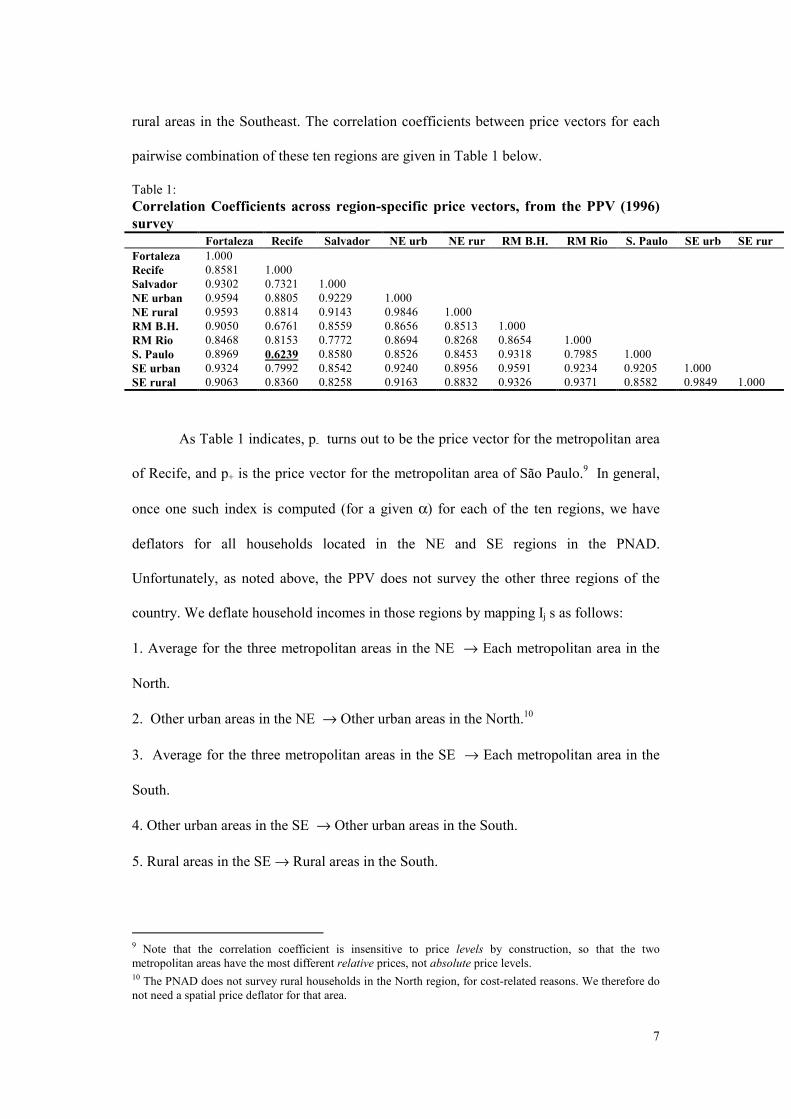
rural areas in the Southeast. The correlation coefficients between price vectors for each
pairwise combination of these ten regions are given in Table 1 below.
Table 1: Correlation Coefficients across region-specific price vectors, from the PPV (1996) survey Fortaleza Recife Salvador NE urb NE rur RM B.H. RM Rio S. Paulo SE urb SE rur Fortaleza 1.000 Recife 0.8581 1.000 Salvador 0.9302 0.7321 1.000 NE urban 0.9594 0.8805 0.9229 1.000 NE rural 0.9593 0.8814 0.9143 0.9846 1.000 RM B.H. 0.9050 0.6761 0.8559 0.8656 0.8513 1.000 RM Rio 0.8468 0.8153 0.7772 0.8694 0.8268 0.8654 1.000 S. Paulo 0.8969 0.6239 0.8580 0.8526 0.8453 0.9318 0.7985 1.000 SE urban 0.9324 0.7992 0.8542 0.9240 0.8956 0.9591 0.9234 0.9205 1.000 SE rural 0.9063 0.8360 0.8258 0.9163 0.8832 0.9326 0.9371 0.8582 0.9849 1.000
As Table 1 indicates, p- turns out to be the price vector for the metropolitan area
of Recife, and p+ is the price vector for the metropolitan area of São Paulo.9 In general,
once one such index is computed (for a given α) for each of the ten regions, we have
deflators for all households located in the NE and SE regions in the PNAD.
Unfortunately, as noted above, the PPV does not survey the other three regions of the
country. We deflate household incomes in those regions by mapping Ij s as follows:
1. Average for the three metropolitan areas in the NE → Each metropolitan area in the
North.
2. Other urban areas in the NE → Other urban areas in the North.10
3. Average for the three metropolitan areas in the SE → Each metropolitan area in the
South.
4. Other urban areas in the SE → Other urban areas in the South.
5. Rural areas in the SE → Rural areas in the South.
9 Note that the correlation coefficient is insensitive to price levels by construction, so that the two metropolitan areas have the most different relative prices, not absolute price levels. 10 The PNAD does not survey rural households in the North region, for cost-related reasons. We therefore do not need a spatial price deflator for that area.
8
6. Average for all metropolitan areas in the NE and SE → Each metropolitan area in the
Center-West.
7. Average of other urban areas across the NE and SE → Other urban areas in the Center-
West.
8. Average of rural areas across the NE and SE → Rural areas in the Center-West.11
This would give us a complete set of price deflators (for any given α), with
which to adjust the entire PNAD household income distribution to take spatial price
differences into account. Furthermore, by varying α in the interval [0, 1], thereby
constructing convex combinations of the two price indices based on the reference regions
with the least correlated price vectors, we could test the robustness of the poverty profile
– or indeed of any poverty or inequality measure – with respect to changes in the choice
of price deflator.
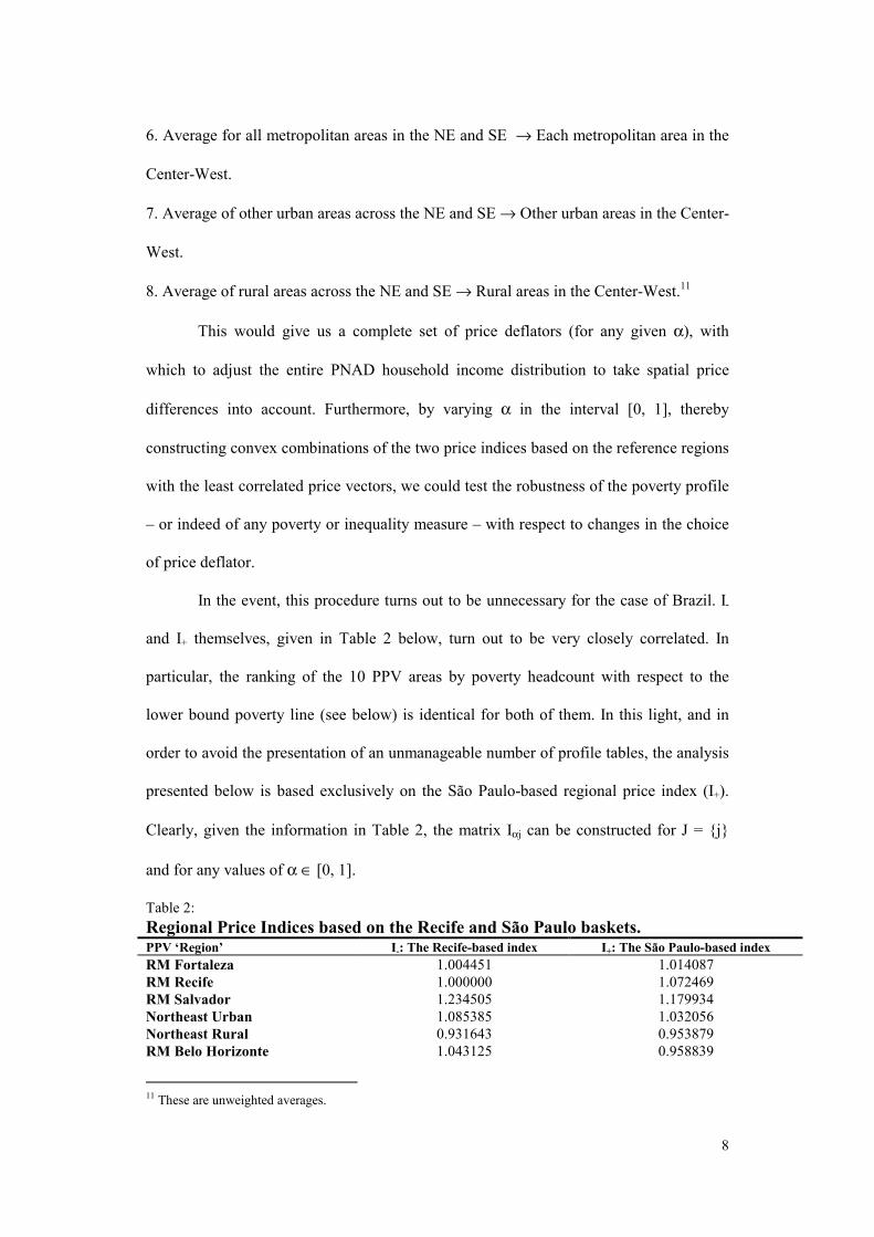
In the event, this procedure turns out to be unnecessary for the case of Brazil. I-
and I+ themselves, given in Table 2 below, turn out to be very closely correlated. In
particular, the ranking of the 10 PPV areas by poverty headcount with respect to the
lower bound poverty line (see below) is identical for both of them. In this light, and in
order to avoid the presentation of an unmanageable number of profile tables, the analysis
presented below is based exclusively on the São Paulo-based regional price index (I+).
Clearly, given the information in Table 2, the matrix Iαj can be constructed for J = {j}
and for any values of α ∈ [0, 1].
Table 2: Regional Price Indices based on the Recife and São Paulo baskets. PPV ‘Region’ I-: The Recife-based index I+: The São Paulo-based index RM Fortaleza 1.004451 1.014087 RM Recife 1.000000 1.072469 RM Salvador 1.234505 1.179934 Northeast Urban 1.085385 1.032056 Northeast Rural 0.931643 0.953879 RM Belo Horizonte 1.043125 0.958839
11 These are unweighted averages.
9
RM Rio de Janeiro 1.094239 1.002163 RM São Paulo 1.120113 1.000000 Southeast Urban 0.995397 0.904720 Southeast Rural 0.985787 0.889700
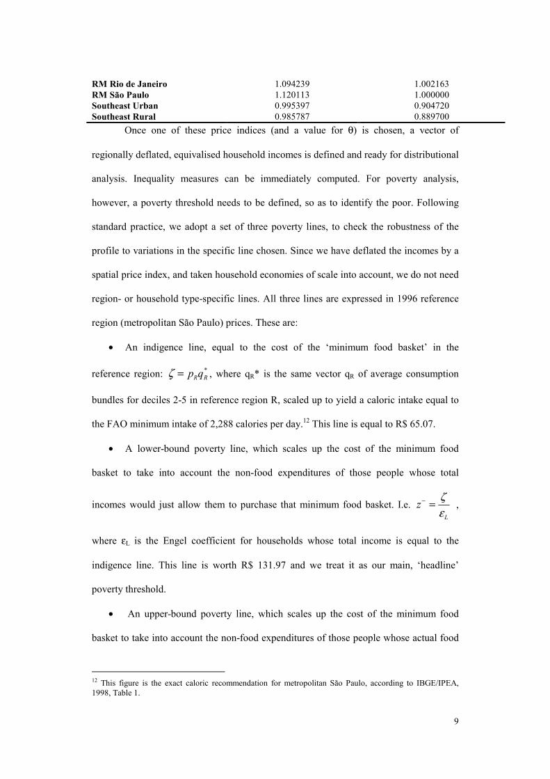
Once one of these price indices (and a value for θ) is chosen, a vector of
regionally deflated, equivalised household incomes is defined and ready for distributional
analysis. Inequality measures can be immediately computed. For poverty analysis,
however, a poverty threshold needs to be defined, so as to identify the poor. Following
standard practice, we adopt a set of three poverty lines, to check the robustness of the
profile to variations in the specific line chosen. Since we have deflated the incomes by a
spatial price index, and taken household economies of scale into account, we do not need
region- or household type-specific lines. All three lines are expressed in 1996 reference
region (metropolitan São Paulo) prices. These are:
• An indigence line, equal to the cost of the ‘minimum food basket’ in the
reference region: ζ = p qR R* , where qR* is the same vector qR of average consumption
bundles for deciles 2-5 in reference region R, scaled up to yield a caloric intake equal to
the FAO minimum intake of 2,288 calories per day.12 This line is equal to R$ 65.07.
• A lower-bound poverty line, which scales up the cost of the minimum food
basket to take into account the non-food expenditures of those people whose total
incomes would just allow them to purchase that minimum food basket. I.e. L
zεζ=− ,
where εL is the Engel coefficient for households whose total income is equal to the
indigence line. This line is worth R$ 131.97 and we treat it as our main, ‘headline’
poverty threshold.
• An upper-bound poverty line, which scales up the cost of the minimum food
basket to take into account the non-food expenditures of those people whose actual food
12 This figure is the exact caloric recommendation for metropolitan São Paulo, according to IBGE/IPEA, 1998, Table 1.
10
expenditures equal the cost of the minimum food basket. I.e. zU
+ = ζε
, where εU is the
Engel coefficient for households whose total food expenditure is equal to the indigence
line. This line is equal to R$ 204.05. While profiles were computed with respect to this
line as well, it yields very high headcounts (62% for Brazil as a whole) and is thus less
useful for profiling. To save space, detailed profiles are not presented for this poverty
line, although results are available from the authors on request.
Since our identification methodology relies on comparing a vector of spatially
deflated incomes with a single poverty line, it is crucial that the poverty line be expressed
in the same ‘currency unit’ as the income vector - i.e. in the 1996 prices ruling in the
reference region (metropolitan São Paulo). If the price deflator changed, the poverty lines
should change in tandem, by adopting the new reference region’s price vector, and
scaling up its quantities vector to yield the desired caloric intake.
3. THE 1996 POVERTY PROFILE: CROSS-TABULATIONS
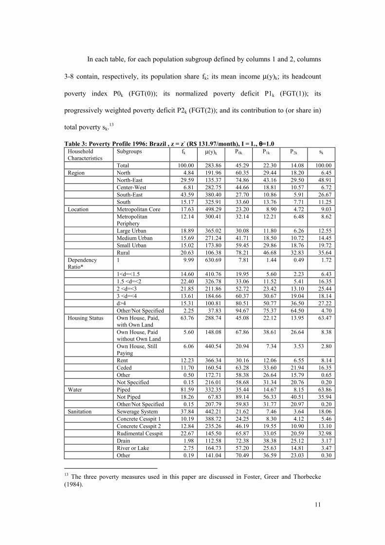
Table 3 below summarizes the results of the poverty profile cross-tabulations
constructed from the adjusted PNAD data set discussed in Section 2, for Brazil as a
whole. As stated above, the Table is based on household income vectors spatially
deflated by the São Paulo-based price index (I+), and for θ = 1.0. Table 3 measures
poverty with respect to the main (lower-bound) poverty line (z- = R$131.97). Table A1 in
the Appendix does so with respect to the indigence line (ζ = R$65.07). Identical profiles
were constructed for the upper-bound poverty line (z+), and these can be obtained from
the authors on request. Since poverty in Brazil, when measured with respect to that line,
is too high to be of much use in identifying the neediest, as well as due to space
constraints, it is not included here.
11
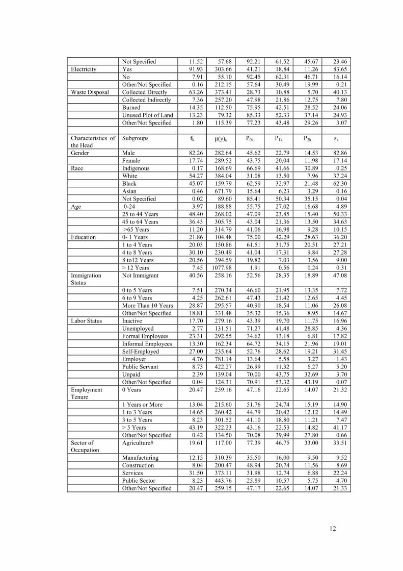
In each table, for each population subgroup defined by columns 1 and 2, columns
3-8 contain, respectively, its population share fk; its mean income µ(y)k; its headcount
poverty index P0k (FGT(0)); its normalized poverty deficit P1k (FGT(1)); its
progressively weighted poverty deficit P2k (FGT(2)); and its contribution to (or share in)
total poverty sk.13
Table 3: Poverty Profile 1996: Brazil , z = z- (R$ 131.97/month), I = I+, θθθθ=1.0 Household Characteristics
Subgroups fk µ(y)k P0k P1k P2k sk
Total 100.00 283.86 45.29 22.30 14.08 100.00 Region North 4.84 191.96 60.35 29.44 18.20 6.45 North-East 29.59 135.37 74.86 43.16 29.50 48.91 Center-West 6.81 282.75 44.66 18.81 10.57 6.72 South-East 43.59 380.40 27.70 10.86 5.91 26.67 South 15.17 325.91 33.60 13.76 7.71 11.25 Location Metropolitan Core 17.63 498.29 23.20 8.90 4.72 9.03 Metropolitan
Periphery 12.14 300.41 32.14 12.21 6.48 8.62
Large Urban 18.89 365.02 30.08 11.80 6.26 12.55 Medium Urban 15.69 271.24 41.71 18.50 10.72 14.45 Small Urban 15.02 173.80 59.45 29.86 18.76 19.72 Rural 20.63 106.38 78.21 46.68 32.83 35.64 Dependency Ratio*
1 9.99 630.69 7.81 1.44 0.49 1.72
1<d=<1.5 14.60 410.76 19.95 5.60 2.23 6.43 1.5 <d=<2 22.40 326.78 33.06 11.52 5.41 16.35 2 <d=<3 21.85 211.86 52.72 23.42 13.10 25.44 3 <d=<4 13.61 184.66 60.37 30.67 19.04 18.14 d>4 15.31 100.81 80.51 50.77 36.50 27.22 Other/Not Specified 2.25 37.83 94.67 75.37 64.50 4.70 Housing Status Own House, Paid,
with Own Land 63.76 288.74 45.08 22.12 13.95 63.47
Own House, Paid without Own Land
5.60 148.08 67.86 38.61 26.64 8.38
Own House, Still Paying
6.06 440.54 20.94 7.34 3.53 2.80
Rent 12.23 366.34 30.16 12.06 6.55 8.14 Ceded 11.70 160.54 63.28 33.60 21.94 16.35 Other 0.50 172.71 58.38 26.64 15.79 0.65 Not Specified 0.15 216.01 58.68 31.34 20.76 0.20 Water Piped 81.59 332.35 35.44 14.67 8.15 63.86 Not Piped 18.26 67.83 89.14 56.33 40.51 35.94 Other/Not Specified 0.15 207.79 59.83 31.77 20.97 0.20 Sanitation Sewerage System 37.84 442.21 21.62 7.46 3.64 18.06 Concrete Cesspit 1 10.19 388.72 24.25 8.30 4.12 5.46 Concrete Cesspit 2 12.84 235.26 46.19 19.55 10.90 13.10 Rudimental Cesspit 22.67 145.50 65.87 33.05 20.59 32.98 Drain 1.98 112.58 72.38 38.38 25.12 3.17 River or Lake 2.75 164.73 57.20 25.63 14.81 3.47 Other 0.19 141.04 70.49 36.59 23.03 0.30
13 The three poverty measures used in this paper are discussed in Foster, Greer and Thorbecke (1984).
12
Not Specified 11.52 57.68 92.21 61.52 45.67 23.46 Electricity Yes 91.93 303.66 41.21 18.84 11.26 83.65 No 7.91 55.10 92.45 62.31 46.71 16.14 Other/Not Specified 0.16 212.15 57.64 30.49 19.99 0.21 Waste Disposal Collected Directly 63.26 373.41 28.73 10.88 5.70 40.13 Collected Indirectly 7.36 257.20 47.98 21.86 12.75 7.80 Burned 14.35 112.50 75.95 42.51 28.52 24.06 Unused Plot of Land 13.23 79.32 85.33 52.33 37.14 24.93 Other/Not Specified 1.80 115.39 77.23 43.48 29.26 3.07 Characteristics of the Head
Subgroups fk µ(y)k P0k P1k P2k sk
Gender Male 82.26 282.64 45.62 22.79 14.53 82.86 Female 17.74 289.52 43.75 20.04 11.98 17.14 Race Indigenous 0.17 168.69 66.69 41.66 30.89 0.25 White 54.27 384.04 31.08 13.50 7.96 37.24 Black 45.07 159.79 62.59 32.97 21.48 62.30 Asian 0.46 671.79 15.64 6.23 3.29 0.16 Not Specified 0.02 89.60 85.41 50.34 35.15 0.04 Age 0-24 3.97 188.88 55.75 27.02 16.68 4.89 25 to 44 Years 48.40 268.02 47.09 23.85 15.40 50.33 45 to 64 Years 36.43 305.75 43.04 21.36 13.50 34.63 >65 Years 11.20 314.79 41.06 16.98 9.28 10.15 Education 0- 1 Years 21.86 104.48 75.00 42.29 28.63 36.20 1 to 4 Years 20.03 150.86 61.51 31.75 20.51 27.21 4 to 8 Years 30.10 230.49 41.04 17.31 9.84 27.28 8 to12 Years 20.56 394.59 19.82 7.03 3.56 9.00 > 12 Years 7.45 1077.98 1.91 0.56 0.24 0.31 Immigration Status
Not Immigrant 40.56 258.16 52.56 28.35 18.89 47.08
0 to 5 Years 7.51 270.34 46.60 21.95 13.35 7.72 6 to 9 Years 4.25 262.61 47.43 21.42 12.65 4.45 More Than 10 Years 28.87 295.57 40.90 18.54 11.06 26.08 Other/Not Specified 18.81 331.48 35.32 15.36 8.95 14.67 Labor Status Inactive 17.70 279.16 43.39 19.70 11.75 16.96 Unemployed 2.77 131.51 71.27 41.48 28.85 4.36 Formal Employees 23.31 292.55 34.62 13.18 6.81 17.82 Informal Employees 13.30 162.34 64.72 34.15 21.96 19.01 Self-Employed 27.00 235.64 52.76 28.62 19.21 31.45 Employer 4.76 781.14 13.64 5.58 3.27 1.43 Public Servant 8.73 422.27 26.99 11.32 6.27 5.20 Unpaid 2.39 139.04 70.00 43.75 32.69 3.70 Other/Not Specified 0.04 124.31 70.91 53.32 43.19 0.07 Employment Tenure
0 Years 20.47 259.16 47.16 22.65 14.07 21.32
1 Years or More 13.04 215.60 51.76 24.74 15.19 14.90 1 to 3 Years 14.65 260.42 44.79 20.42 12.12 14.49 3 to 5 Years 8.23 301.52 41.10 18.80 11.21 7.47 > 5 Years 43.19 322.23 43.16 22.53 14.82 41.17 Other/Not Specified 0.42 134.50 70.08 39.99 27.80 0.66 Sector of Occupation
Agriculture# 19.61 117.00 77.39 46.75 33.00 33.51
Manufacturing 12.15 310.39 35.50 16.00 9.50 9.52 Construction 8.04 200.47 48.94 20.74 11.56 8.69 Services 31.50 373.11 31.98 12.74 6.88 22.24 Public Sector 8.23 443.76 25.89 10.57 5.75 4.70 Other/Not Specified 20.47 259.15 47.17 22.65 14.07 21.33
13
Notes: s f PPk
k ok=0
. Dependency ratio is defined as the number of household members over the number of
earners in the household. # Agriculture includes other Primary Sector occupations. Table 3 contains a substantial amount of descriptive information. We discuss it
under three main headings: the spatial profile; characteristics of the head; and housing
and access to services.
The Spatial Profile
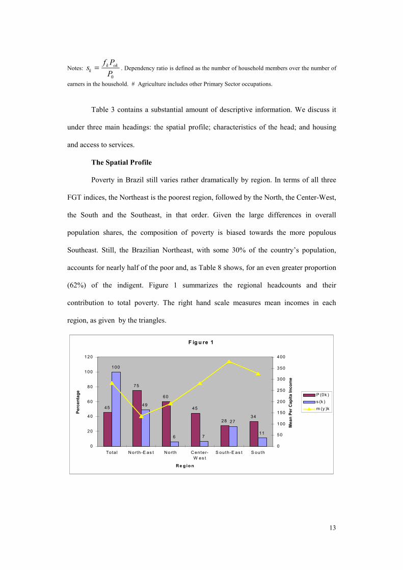
Poverty in Brazil still varies rather dramatically by region. In terms of all three
FGT indices, the Northeast is the poorest region, followed by the North, the Center-West,
the South and the Southeast, in that order. Given the large differences in overall
population shares, the composition of poverty is biased towards the more populous
Southeast. Still, the Brazilian Northeast, with some 30% of the country’s population,
accounts for nearly half of the poor and, as Table 8 shows, for an even greater proportion
(62%) of the indigent. Figure 1 summarizes the regional headcounts and their
contribution to total poverty. The right hand scale measures mean incomes in each
region, as given by the triangles.
F ig u re 1
100
3428
45
60
75
45
11
27
76
49
0
20
40
60
80
100
120
Tota l N orth -E as t N orth C enter-W es t
S outh-E as t S outh
R e g io n
Perc
enta
ge
0
50
100
150
200
250
300
350
400
Mea
n Pe
r Cap
ita In
com
e
P (0k )s (k )m (y )k
14
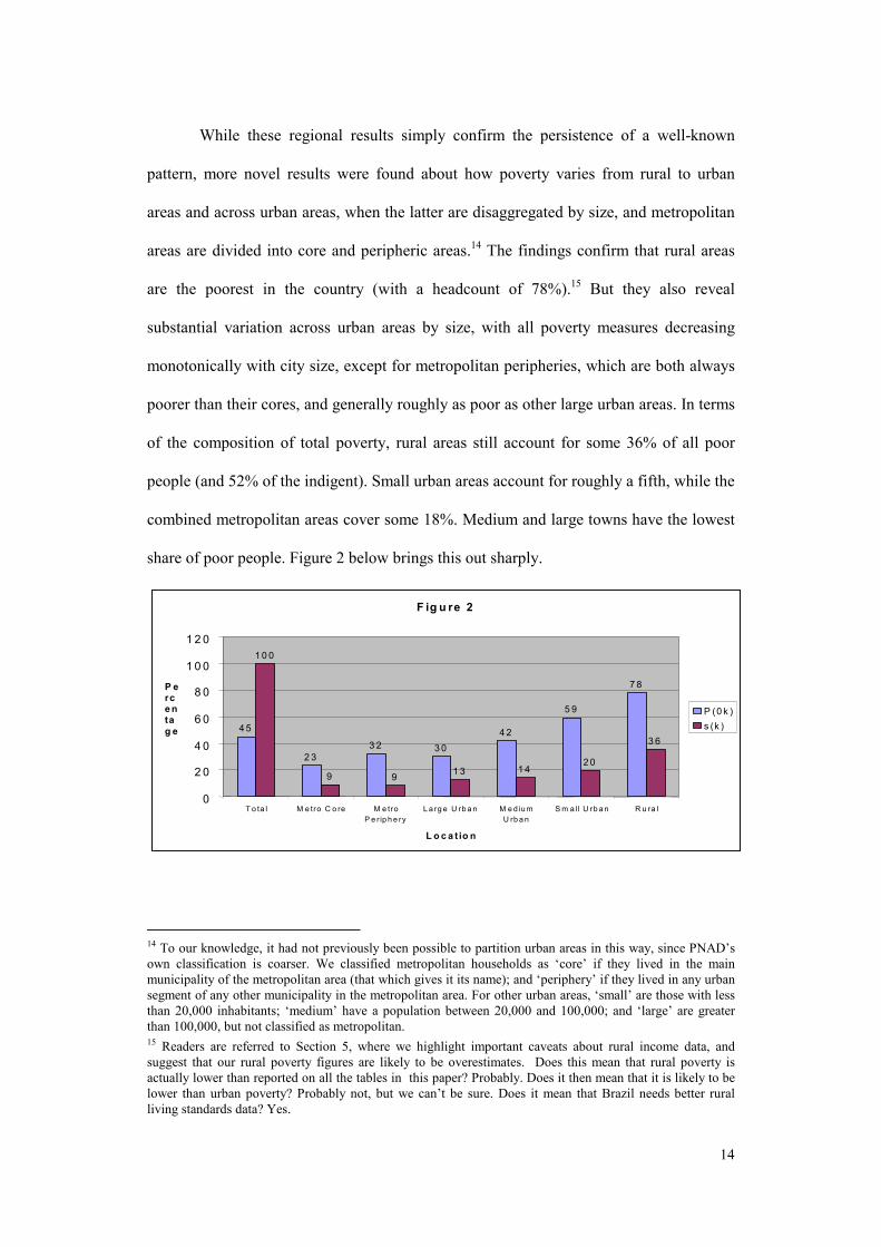
While these regional results simply confirm the persistence of a well-known
pattern, more novel results were found about how poverty varies from rural to urban
areas and across urban areas, when the latter are disaggregated by size, and metropolitan
areas are divided into core and peripheric areas.14 The findings confirm that rural areas
are the poorest in the country (with a headcount of 78%).15 But they also reveal
substantial variation across urban areas by size, with all poverty measures decreasing
monotonically with city size, except for metropolitan peripheries, which are both always
poorer than their cores, and generally roughly as poor as other large urban areas. In terms
of the composition of total poverty, rural areas still account for some 36% of all poor
people (and 52% of the indigent). Small urban areas account for roughly a fifth, while the
combined metropolitan areas cover some 18%. Medium and large towns have the lowest
share of poor people. Figure 2 below brings this out sharply.
F ig u re 2
1 0 0
7 8
5 9
4 23 03 2
2 3
4 53 6
2 01 41 399
0
2 0
4 0
6 0
8 0
1 0 0
1 2 0
T o ta l M e tro C o re M e troP e r ip h e ry
L a rg e U rb a n M e d iu mU rb a n
S m a ll U rb a n R u ra l
L o c a t io n
P erce ntag e
P (0 k )s (k )
14 To our knowledge, it had not previously been possible to partition urban areas in this way, since PNAD’s own classification is coarser. We classified metropolitan households as ‘core’ if they lived in the main municipality of the metropolitan area (that which gives it its name); and ‘periphery’ if they lived in any urban segment of any other municipality in the metropolitan area. For other urban areas, ‘small’ are those with less than 20,000 inhabitants; ‘medium’ have a population between 20,000 and 100,000; and ‘large’ are greater than 100,000, but not classified as metropolitan. 15 Readers are referred to Section 5, where we highlight important caveats about rural income data, and suggest that our rural poverty figures are likely to be overestimates. Does this mean that rural poverty is actually lower than reported on all the tables in this paper? Probably. Does it then mean that it is likely to be lower than urban poverty? Probably not, but we can’t be sure. Does it mean that Brazil needs better rural living standards data? Yes.
15
The policy implications of this disaggregation of urban poverty are not
insubstantial. In the first place, poverty incidence is far higher in small and medium
towns than in the metropolitan regions, and policies to combat urban poverty should be
targeted accordingly. The common view of placid country-side towns as idyllic when
compared to the peripheries of large cities appears to be wide of the mark, and any
comprehensive strategy for poverty reduction must focus both on rural areas and on small
and medium-sized towns. Second, poverty incidence within metropolitan areas is higher
outside the central municipality. Not only is poverty in metropolitan areas less severe
than in smaller towns, but it must be combated beginning from their outlying peripheries.
Characteristics of the Household Head.
Turning now to population partitions based on characteristics of the household
head, we find first that male- and female-headed households do not really differ in the
extent to which they are likely to be poor. This is not as surprising as might appear, and
confirms previous findings for Brazil and other developing countries.16 It should not,
however, be taken to mean that the ‘average welfare’ of men and women in Brazil is
roughly the same. This comparison relies on the (narrow) concept of household headship,
and says nothing about gender wage gaps in the labor market, or indeed about the intra-
household distribution of resources. On both of these important areas, there is evidence
to suggest that women may fare less well than men.17
Race seems to matter a great deal more. The mean income in black-headed
households is 42% of that in white-headed households, and only 24% of that for Asian-
headed households. The ratios are very similar for indigenous-headed households. As a
result, the headcount for black-headed households, at 63%, is roughly double that for
16 See Ferreira and Litchfield (2001) and Neri and Camargo (2002) on inequality decompositions for Brazil, and Quisumbing et. al. (1995) on welfare comparisons across male- and female-headed households for a sample of developing countries. 17 See Deaton (1989) on a pathbreaking investigation of intra-household resource allocation, and Amadeo et. al. (1994) on the level of and changes in the gender gap in the Brazilian labor market.
16
whites, and four times that for Asians. Despite being a (large) minority, black-headed
households account for 62% of all poor people in Brazil (ranging from 24% in the South,
to 78% in the North). This leaves no room for doubt that the small Asian minority and
the white majority are, on average, at a considerably smaller risk of poverty than their
black or indigenous counterparts in Brazil. However, the probit analysis discussed in the
next section reveals that the marginal effect of race is statistically insignificant when one
controls for other relevant variables, such as years of schooling, region, family size and
composition. The conclusion must be that, while there is no doubt about the (descriptive)
average association between race and poverty, further work is needed to establish the
mechanisms through which race affects household welfare outcomes. It is quite likely
that some of it operates through educational attainment or demographic choices, but
labor market and other forms of discrimination can certainly not be ruled out.
The age of the household head displays a small but perceptible (unconditional)
correlation with poverty incidence. The latter declines monotonically with age, according
to the partition in Table 3. Perhaps the most interesting part of this association, which is
otherwise in line with conventional wisdom on labor market returns to experience (often
proxied by age), is that it persists for household heads older than 65. These households
have the highest mean income of any age group. Since this profile is based on current
incomes, this seems to contradict the permanent income hypothesis implication that these
older households should be earning less and dissaving into their retirement years. This
may reflect a higher life expectancy among richer people; or indeed an excessively
generous (and regressive) pension system in operation.18
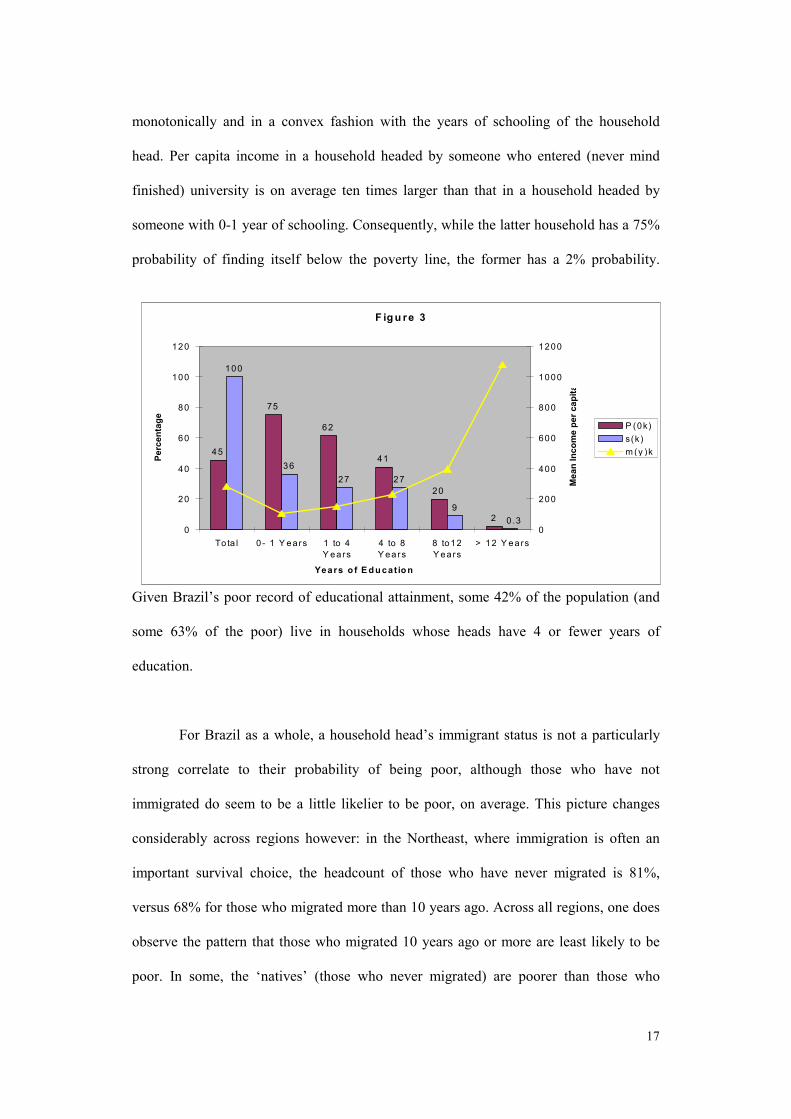
As usual, the most significant (inverse) correlate of poverty is the education of
the household head. As Table 3 and Figure 3 below indicate, household income rises
18 See Neri et all. (1999), Neri (2001), Hoffman (2001) and Bourguignon, Ferreira and Leite (2002) on the incidence of Brazilian retirement pensions.
17
monotonically and in a convex fashion with the years of schooling of the household
head. Per capita income in a household headed by someone who entered (never mind
finished) university is on average ten times larger than that in a household headed by
someone with 0-1 year of schooling. Consequently, while the latter household has a 75%
probability of finding itself below the poverty line, the former has a 2% probability.
Given Brazil’s poor record of educational attainment, some 42% of the population (and
some 63% of the poor) live in households whose heads have 4 or fewer years of
education.
For Brazil as a whole, a household head’s immigrant status is not a particularly
strong correlate to their probability of being poor, although those who have not
immigrated do seem to be a little likelier to be poor, on average. This picture changes
considerably across regions however: in the Northeast, where immigration is often an
important survival choice, the headcount of those who have never migrated is 81%,
versus 68% for those who migrated more than 10 years ago. Across all regions, one does
observe the pattern that those who migrated 10 years ago or more are least likely to be
poor. In some, the ‘natives’ (those who never migrated) are poorer than those who
F ig u re 3
75
100
92
20
41
62
45
0 .3
272736
0
20
40
60
80
100
120
To ta l 0 - 1 Y ears 1 to 4Y ears
4 to 8Y ears
8 to12Y ears
> 12 Y ears
Years o f E d u cat io n
Perc
enta
ge
0
200
400
600
800
1000
1200
Mea
n In
com
e pe
r cap
ita
P (0k)s(k)m (y )k
18
migrated between 1 and 9 years ago (like the Northeast), and in others they are richer
(like in the South).
As regards labor status, the unemployed and the informal employees (‘sem
carteira’) have the highest headcounts, followed by the self-employed. Formal employees
(‘com carteira’) are roughly half as likely to be poor (35%) as their informal counterparts
(65%). Although poverty among the unemployed records the highest values for all three
poverty measures, the labor category contributing the largest share of overall poverty is
that of the self-employed, since they are ten times as numerous in Brazil as the
unemployed (in 1996). This poverty incidence and severity profile by labor status
confirms that recent increases in unemployment are a serious cause for concern about
poverty and welfare among the households of those affected. However, the numerical
predominance of self-employed workers, allied to the fact that they too are likely to
suffer from reductions in aggregate demand, should serve as a reminder that they should
not be neglected in the design of safety nets and other remedial policies.
The figures for sector of occupation reveal, once again, the prevalence of poverty
among agricultural workers.19 Among predominantly urban sectors, construction has
poorer workers than both manufacturing and services. Public sector workers and
employers are, on average, least likely to see their households in poverty.
Housing Characteristics and Access to Services
This part of the profile is clearly even less amenable to any causal interpretation.
It is intended merely to describe some of the living conditions of the poor, as compared
to the non-poor. Housing status, for instance, provides an interesting insight into the
Brazilian housing market. Unlike in many developed countries, where poorer households
rent, and the richest ones own houses outright, the highest mean incomes in Brazil are
19 Although, once again, the reader is reminded that poverty rates for agricultural workers are likely to be overestimated due to faulty data collection. See Section 3.
19
amongst those who rent and those who pay mortgages. The lowest mean incomes are
those for households living in ‘ceded’ housing20 (some 12% of the population), and those
who own their houses, but not the land they are built on. The headcounts in these two
categories is between 60% and 70%.
However, given their population share, the vast majority of those counted as poor
in table 7 (63% of them) own both their houses and the land on which they stand. This
confirms the anecdotal evidence of middle-class households renting flats in the
fashionable Jardins neighborhood in São Paulo, or in Rio’s ‘Zona Sul’, while their
domestic servants may own a house in a distant part of the metropolitan periphery. The
latter may often have been built through a community effort (‘mutirão’), using second-
rate materials, and with facilities which are considerably less comfortable. But they and
the plot of land they are in are owned by the residents.21 Whether this reflects different
preferences, or capital and land market failures, which prevent the poor from accessing
either the mortgage or the mainstream rental markets, must remain a matter for further
study.
As for access to services, 18% of the Brazilian population (36% of the poor) do
not have access to piped water. Only 18 % of the poor (versus 38% overall) dispose of
their sewage through the main sewerage system. The remaining 82% use alternative
means, such as cesspits, drains or direct dumping on river or lakes. 16% of poor
households have no access to electricity, as compared to 8% of the total population. And
a full 49% of the poor dispose of their garbage by either burning it or dumping it in an
unused plot of land. The policy implications from this paragraph dispense with detailed
spelling out.
20 ‘Ceded” housing is an arrangement predominant in some types of agricultural contracts and among domestic servants. 21 Note that the ownership question in the PNAD does not explicitly specify formal ownership, and it remains unclear whether all those reporting ownership are necessarily in possession of an official land title.
20
A profile which is exactly analogous to the one just presented, but computed with
respect to the indigence line (ζ) of R$ 65.07 per person per month, is presented in Table
A1 in the Appendix. The broad patterns of the profile (though clearly not the values of
the poverty measures) do not change much across the two poverty lines. The main
features of Table A1 have already been incorporated into the above discussion.
4. THE 1996 POVERTY PROFILE: AN ANALYSIS OF MARGINAL EFFECTS.
While the cross-tabulations presented in the previous section are informative,
they have two shortcomings. First, the simple associations between personal
characteristics and different measures of poverty are essentially bivariate, and do not
control for the effects of other variables. Second, the long tables are not wieldy to test the
robustness of the profile with respect to changes in spatial price deflation or in the
assumptions about scale economies within households, which was one of the advantages
of the methodology proposed in Section 2. We therefore conduct the robustness tests in a
‘marginal effect’ version of the profile, given by simple transformations of a probit
model, regressing the probability of being poor on the relevant household characteristics
which were used in the cross-tabulations.22 In this exercise, poverty statistics are
computed from income data in the PPV sample, and all covariates come from the same
source.
These profile probit regressions are intended to be merely descriptive, and no
inference of causation whatsoever is made. The transformed coefficients should be seen
only as estimates of partial correlation coefficients with the probability of being poor.
The vector of independent variables X includes the following household variables:
22 As θ varies, we scale the poverty line up by a factor equal to
θ−1n , where n is the average household
size, so as to keep the overall poverty incidence rate constant for households with the average household size. This allows us to compensate for the pure size effect of the adjustment to the income effect, while preserving the re-rankings which are an important part of the exercise.
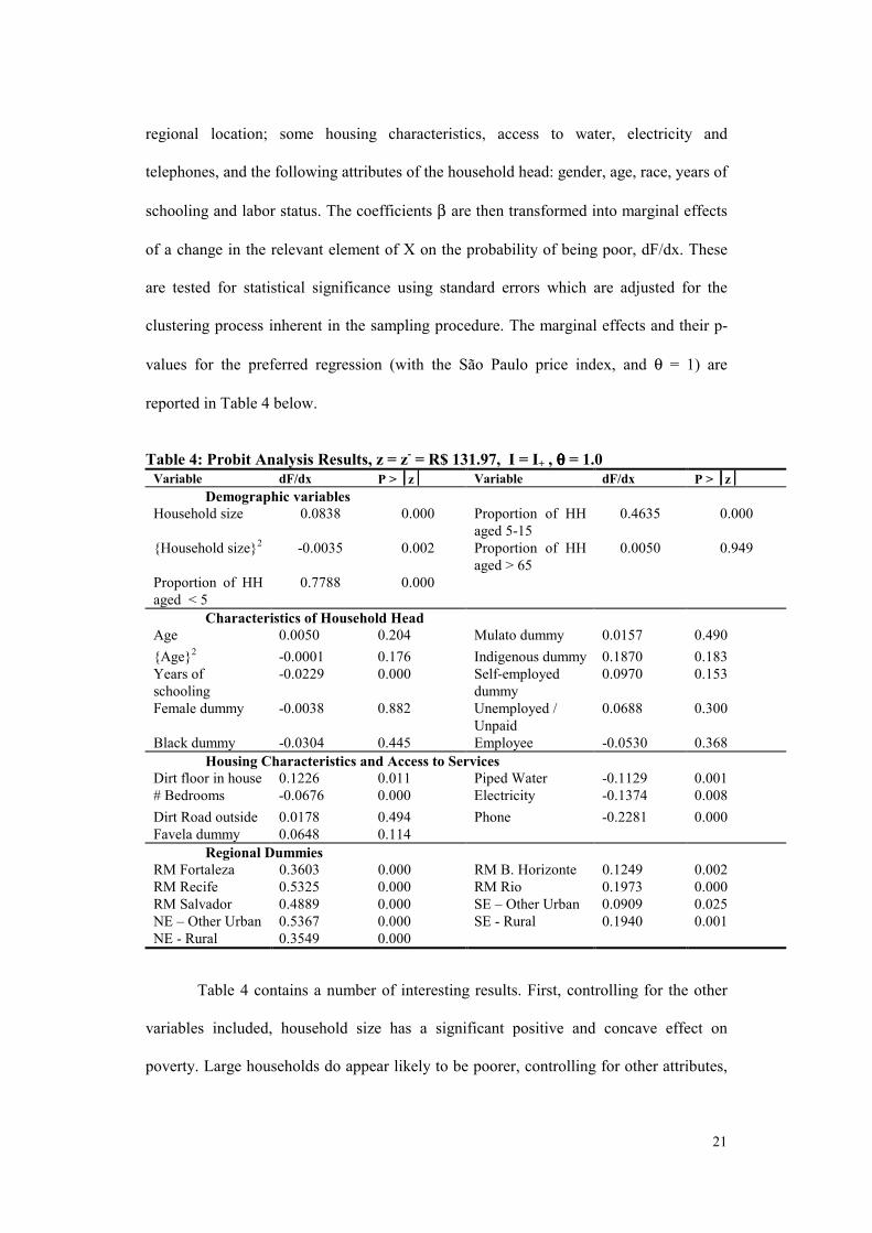
21
regional location; some housing characteristics, access to water, electricity and
telephones, and the following attributes of the household head: gender, age, race, years of
schooling and labor status. The coefficients β are then transformed into marginal effects
of a change in the relevant element of X on the probability of being poor, dF/dx. These
are tested for statistical significance using standard errors which are adjusted for the
clustering process inherent in the sampling procedure. The marginal effects and their p-
values for the preferred regression (with the São Paulo price index, and θ = 1) are
reported in Table 4 below.
Table 4: Probit Analysis Results, z = z- = R$ 131.97, I = I+ , θθθθ = 1.0
Variable dF/dx P > z Variable dF/dx P > z Demographic variables
Household size 0.0838 0.000 Proportion of HH aged 5-15
0.4635 0.000
{Household size}2 -0.0035 0.002 Proportion of HH aged > 65
0.0050 0.949
Proportion of HH aged < 5
0.7788 0.000
Characteristics of Household Head Age 0.0050 0.204 Mulato dummy 0.0157 0.490 {Age}2 -0.0001 0.176 Indigenous dummy 0.1870 0.183 Years of schooling
-0.0229 0.000 Self-employed dummy
0.0970 0.153
Female dummy -0.0038 0.882 Unemployed / Unpaid
0.0688 0.300
Black dummy -0.0304 0.445 Employee -0.0530 0.368 Housing Characteristics and Access to Services
Dirt floor in house 0.1226 0.011 Piped Water -0.1129 0.001 # Bedrooms -0.0676 0.000 Electricity -0.1374 0.008 Dirt Road outside 0.0178 0.494 Phone -0.2281 0.000 Favela dummy 0.0648 0.114
Regional Dummies RM Fortaleza 0.3603 0.000 RM B. Horizonte 0.1249 0.002 RM Recife 0.5325 0.000 RM Rio 0.1973 0.000 RM Salvador 0.4889 0.000 SE – Other Urban 0.0909 0.025 NE – Other Urban 0.5367 0.000 SE - Rural 0.1940 0.001 NE - Rural 0.3549 0.000
Table 4 contains a number of interesting results. First, controlling for the other
variables included, household size has a significant positive and concave effect on
poverty. Large households do appear likely to be poorer, controlling for other attributes,
22
although the relationship is concave in family size. Similarly, the proportion of children
is positively correlated with poverty, and more strongly so for younger children. No such
significant correlation is found for the proportion of over-65s in the household. These
results are robust not only to different price deflation procedures but also, more
interestingly, to changing the household equivalence scale parameter θ to 0.75. In that
regression, household size remained positive, concave and significant, and the results for
children and the elderly were unchanged. Only when the probit was run for an income
vector adjusted by θ = 0.50, did we observe a reversal in the sign of the marginal effect
of household size, which then became insignificant. This suggests that, unless there are
reasons to suppose that economies of scale within Brazilian households are greater than
those implied by a theta in the (0.7, 1.0) range, the stylized fact that larger households are
poorer, controlling for other attributes, survives scrutiny. Our findings also suggest that a
larger number of children is correlated with a greater probability of being poor, while the
same is not true of a larger number of older people.
Turning then, to the marginal effects of characteristics of household heads, we
find some surprising results. The unsurprising one, of course, is that education is
significantly negatively correlated with the probability of being poor (although, even
here, the effect is quantitatively much smaller than that of living in a richer area). But
apart from education; age, gender, ethnicity and the occupational status of the household
head, all turn out to be insignificant correlates of poverty. For age and gender, this is in
line with previous findings from decompositions of Generalized Entropy inequality
measures (see Ferreira and Litchfield, 2001). It is also confirmed by the tabulation
profiles presented in the previous Section.
Race, however, had appeared to account for a significant share of inequality in
those static inequality decompositions, and the tabulation profiles show substantial
differences between the poverty incidences across households headed by blacks
23
(including ‘mulatos’), and whites. Clearly, the insignificance of the race dummy in the
probits is a result of controlling for the other attributes included in the regression. While
on average, black and indigenous households are substantially more likely to be poor,
this seems to be because of other differences between them and white-headed
households, such as education or regional location. This is not to say that there are no
grounds for poverty reducing policies which take race into account. Neither can it be
interpreted as a verdict on the old sociological debate about whether Brazil’s racism is
more ‘economic’ than ‘social’. All it does say is that if households headed by non-whites
are likelier to be poor, then this is due to their differential access to education, or to their
locational choices, or to some other factor, rather than simply because they are non-
white.
In terms of housing characteristics and access to services, the direction of
causation is almost certainly from poverty to these attributes, rather than the reverse. Our
caveat about interpreting these ‘marginal effects’ merely as descriptive estimates of
partial correlation coefficients is particularly pertinent here. The main result is that the
poor are indeed significantly less likely to have access to piped water, electricity or, even
more markedly, a telephone line. They are also less likely to have many bedrooms, or
covered housing floors. The correlations with the nature of the road or street outside, as
well as to whether the household is located in a slum (‘favela’), turned out to be
insignificant, once other factors are taken into account.
Finally, the effect of regional location on the probability of being poor can only
be described as dramatic. The reference region (missing dummy) is the metropolitan area
of São Paulo. Simply put, the marginal effects reported suggest that living anywhere else
is correlated with a greater likelihood of being poor, though the quantitative effects are
much larger for the Northeast than within the Southeast. Note that these effects have
remained this strongly significant after controlling for differences in education, labor
24
status, housing characteristics, etc. The implication is that regional differences in
household income, and hence in the vulnerability to poverty, are not only a consequence
of different educational attainment levels, demographic differences across regions, or
racial make-up. They must be explained by other factors, which deserve continuing
investigation.
In addition to these results, which are interesting in themselves, the probit
analysis was used to check the robustness of the profile to changes in two aspects of our
adjustments to the data: the regional price deflators, and the Buhmann et. al. equivalence
scale parameter θ, both of which were discussed in section 2.
When no regional price adjustment is used, the marginal effects of variables
other than regional dummies is hardly affected. However, the regional dummies are
affected in the manner one would expect. Places where the cost of living is higher than in
São Paulo (such as Recife or Salvador) have lower marginal effects (since real incomes
there are overestimated in the absence of an adjustment), while areas where the cost of
living is lower than in São Paulo (such as the rural Southeast) have higher marginal
effects, since real incomes there are underestimated. On the other hand, using different
price deflators, such as the São Paulo-based and the Recife-based indices, which were
chosen exactly so as to maximize the difference in relative prices between them, turns
out to have virtually no effect on either the sign or the significance of any of the right-
hand-side variables.
Our conclusions from these robustness checks were twofold. First, dimensions of
the profile which are unrelated to household size do not seem to be affected by the choice
of theta. Second, it does seem that some price deflation, as opposed to none, makes a
difference to the estimated ‘marginal effects’ of living in different areas on poverty. In
other words, not taking spatial cost-of-living differences into account does seem to lead
to some re-rankings in poverty across regions. It therefore seemed advisable to adopt one
25
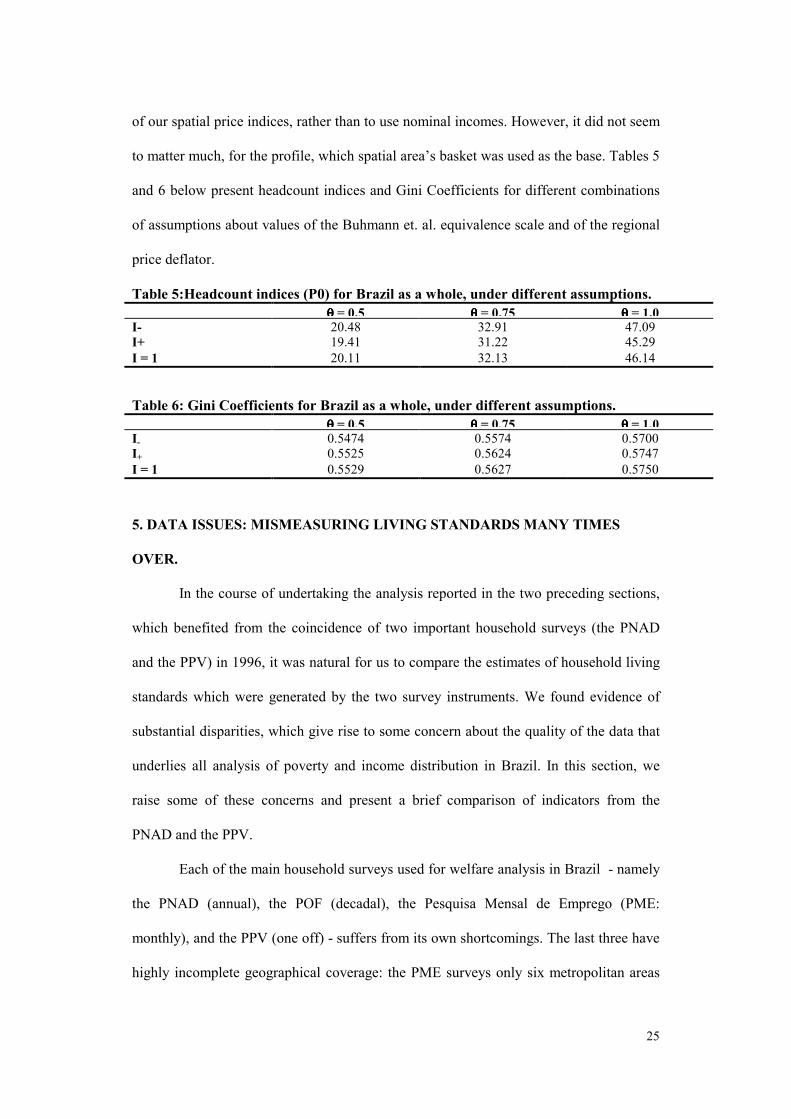
of our spatial price indices, rather than to use nominal incomes. However, it did not seem
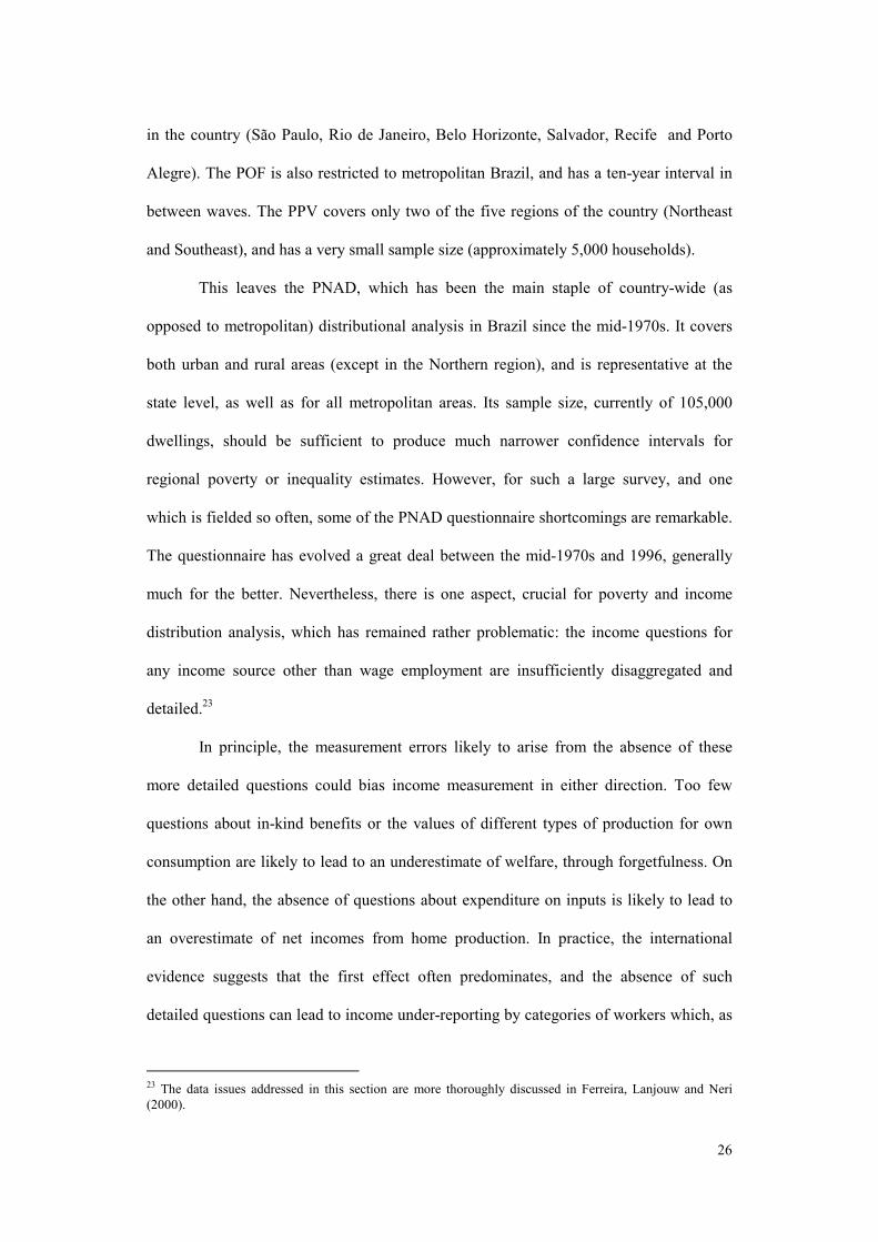
to matter much, for the profile, which spatial area’s basket was used as the base. Tables 5
and 6 below present headcount indices and Gini Coefficients for different combinations
of assumptions about values of the Buhmann et. al. equivalence scale and of the regional
price deflator.
Table 5:Headcount indices (P0) for Brazil as a whole, under different assumptions. θθθθ = 0.5 θθθθ = 0.75 θθθθ = 1.0
I- 20.48 32.91 47.09I+ 19.41 31.22 45.29 I = 1 20.11 32.13 46.14
Table 6: Gini Coefficients for Brazil as a whole, under different assumptions. θθθθ = 0.5 θθθθ = 0.75 θθθθ = 1.0
I- 0.5474 0.5574 0.5700 I+ 0.5525 0.5624 0.5747 I = 1 0.5529 0.5627 0.5750
5. DATA ISSUES: MISMEASURING LIVING STANDARDS MANY TIMES
OVER.
In the course of undertaking the analysis reported in the two preceding sections,
which benefited from the coincidence of two important household surveys (the PNAD
and the PPV) in 1996, it was natural for us to compare the estimates of household living
standards which were generated by the two survey instruments. We found evidence of
substantial disparities, which give rise to some concern about the quality of the data that
underlies all analysis of poverty and income distribution in Brazil. In this section, we
raise some of these concerns and present a brief comparison of indicators from the
PNAD and the PPV.
Each of the main household surveys used for welfare analysis in Brazil - namely
the PNAD (annual), the POF (decadal), the Pesquisa Mensal de Emprego (PME:
monthly), and the PPV (one off) - suffers from its own shortcomings. The last three have
highly incomplete geographical coverage: the PME surveys only six metropolitan areas
26
in the country (São Paulo, Rio de Janeiro, Belo Horizonte, Salvador, Recife and Porto
Alegre). The POF is also restricted to metropolitan Brazil, and has a ten-year interval in
between waves. The PPV covers only two of the five regions of the country (Northeast
and Southeast), and has a very small sample size (approximately 5,000 households).
This leaves the PNAD, which has been the main staple of country-wide (as
opposed to metropolitan) distributional analysis in Brazil since the mid-1970s. It covers
both urban and rural areas (except in the Northern region), and is representative at the
state level, as well as for all metropolitan areas. Its sample size, currently of 105,000
dwellings, should be sufficient to produce much narrower confidence intervals for
regional poverty or inequality estimates. However, for such a large survey, and one
which is fielded so often, some of the PNAD questionnaire shortcomings are remarkable.
The questionnaire has evolved a great deal between the mid-1970s and 1996, generally
much for the better. Nevertheless, there is one aspect, crucial for poverty and income
distribution analysis, which has remained rather problematic: the income questions for
any income source other than wage employment are insufficiently disaggregated and
detailed.23
In principle, the measurement errors likely to arise from the absence of these
more detailed questions could bias income measurement in either direction. Too few
questions about in-kind benefits or the values of different types of production for own
consumption are likely to lead to an underestimate of welfare, through forgetfulness. On
the other hand, the absence of questions about expenditure on inputs is likely to lead to
an overestimate of net incomes from home production. In practice, the international
evidence suggests that the first effect often predominates, and the absence of such
detailed questions can lead to income under-reporting by categories of workers which, as
23 The data issues addressed in this section are more thoroughly discussed in Ferreira, Lanjouw and Neri (2000).
27
it happens, are quite likely to be poor (see, e.g. Lanjouw and Lanjouw, 1996). The
evidence which we have uncovered for Brazil, by comparing incomes and poverty
incidence estimates from the PPV - which contains (a) a consumption expenditure
questionnaire and (b) a more detailed income questionnaire - with the PNAD estimates,
suggests that the same is true in this country.
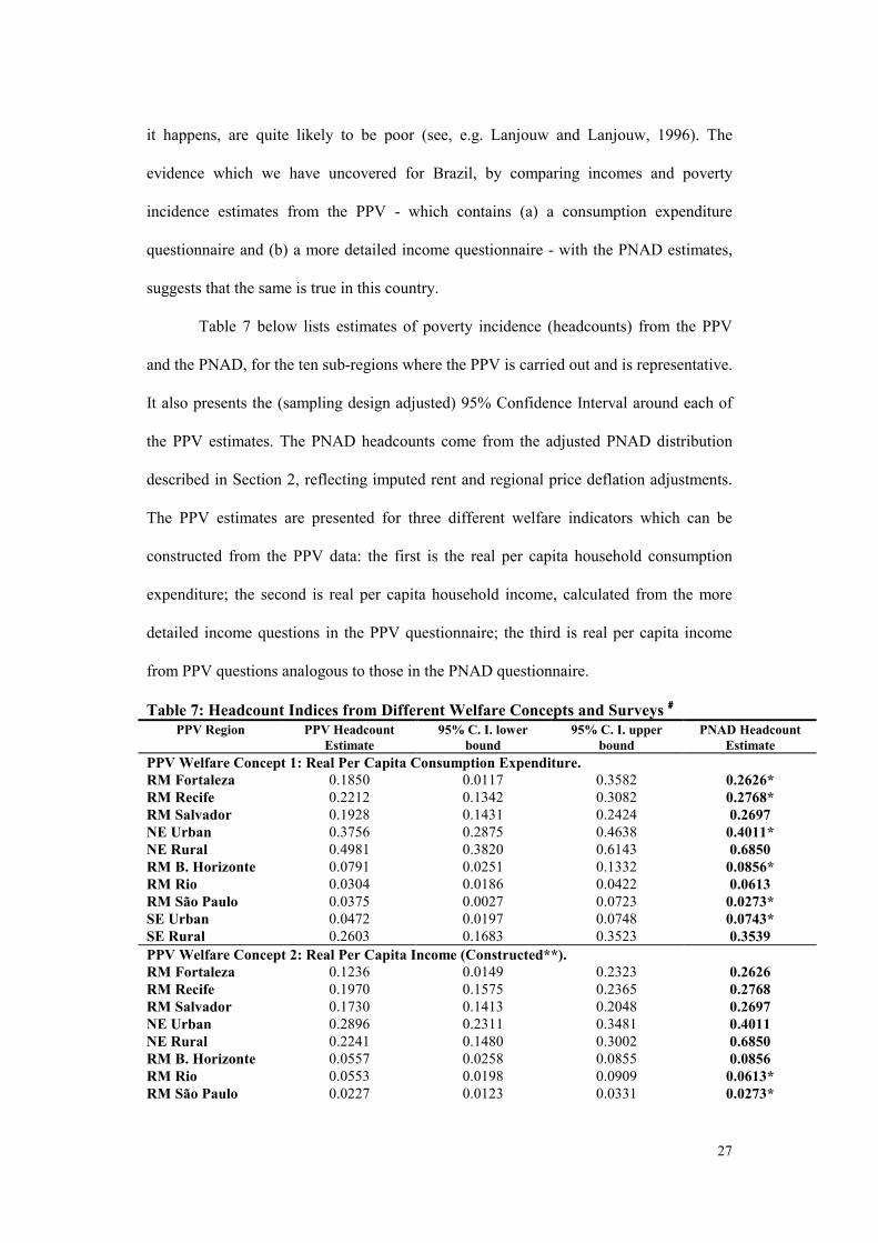
Table 7 below lists estimates of poverty incidence (headcounts) from the PPV
and the PNAD, for the ten sub-regions where the PPV is carried out and is representative.
It also presents the (sampling design adjusted) 95% Confidence Interval around each of
the PPV estimates. The PNAD headcounts come from the adjusted PNAD distribution
described in Section 2, reflecting imputed rent and regional price deflation adjustments.
The PPV estimates are presented for three different welfare indicators which can be
constructed from the PPV data: the first is the real per capita household consumption
expenditure; the second is real per capita household income, calculated from the more
detailed income questions in the PPV questionnaire; the third is real per capita income
from PPV questions analogous to those in the PNAD questionnaire.
Table 7: Headcount Indices from Different Welfare Concepts and Surveys #### PPV Region PPV Headcount
Estimate 95% C. I. lower
bound 95% C. I. upper
bound PNAD Headcount
Estimate PPV Welfare Concept 1: Real Per Capita Consumption Expenditure. RM Fortaleza 0.1850 0.0117 0.3582 0.2626* RM Recife 0.2212 0.1342 0.3082 0.2768* RM Salvador 0.1928 0.1431 0.2424 0.2697 NE Urban 0.3756 0.2875 0.4638 0.4011* NE Rural 0.4981 0.3820 0.6143 0.6850 RM B. Horizonte 0.0791 0.0251 0.1332 0.0856* RM Rio 0.0304 0.0186 0.0422 0.0613 RM São Paulo 0.0375 0.0027 0.0723 0.0273* SE Urban 0.0472 0.0197 0.0748 0.0743* SE Rural 0.2603 0.1683 0.3523 0.3539 PPV Welfare Concept 2: Real Per Capita Income (Constructed**). RM Fortaleza 0.1236 0.0149 0.2323 0.2626 RM Recife 0.1970 0.1575 0.2365 0.2768 RM Salvador 0.1730 0.1413 0.2048 0.2697 NE Urban 0.2896 0.2311 0.3481 0.4011 NE Rural 0.2241 0.1480 0.3002 0.6850 RM B. Horizonte 0.0557 0.0258 0.0855 0.0856 RM Rio 0.0553 0.0198 0.0909 0.0613* RM São Paulo 0.0227 0.0123 0.0331 0.0273*
28
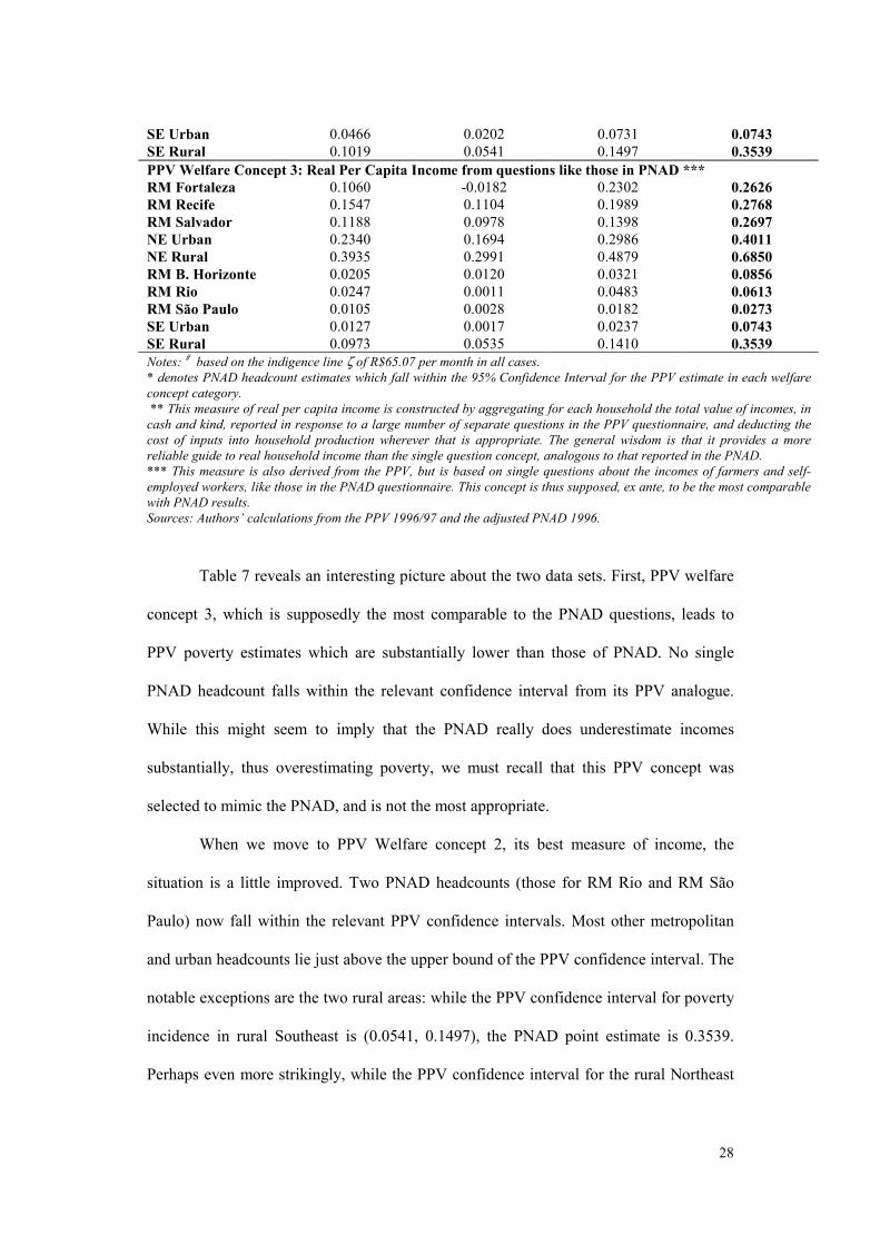
SE Urban 0.0466 0.0202 0.0731 0.0743 SE Rural 0.1019 0.0541 0.1497 0.3539 PPV Welfare Concept 3: Real Per Capita Income from questions like those in PNAD *** RM Fortaleza 0.1060 -0.0182 0.2302 0.2626 RM Recife 0.1547 0.1104 0.1989 0.2768 RM Salvador 0.1188 0.0978 0.1398 0.2697 NE Urban 0.2340 0.1694 0.2986 0.4011 NE Rural 0.3935 0.2991 0.4879 0.6850 RM B. Horizonte 0.0205 0.0120 0.0321 0.0856 RM Rio 0.0247 0.0011 0.0483 0.0613 RM São Paulo 0.0105 0.0028 0.0182 0.0273 SE Urban 0.0127 0.0017 0.0237 0.0743 SE Rural 0.0973 0.0535 0.1410 0.3539 Notes: # based on the indigence line ζ of R$65.07 per month in all cases. * denotes PNAD headcount estimates which fall within the 95% Confidence Interval for the PPV estimate in each welfare concept category. ** This measure of real per capita income is constructed by aggregating for each household the total value of incomes, in cash and kind, reported in response to a large number of separate questions in the PPV questionnaire, and deducting the cost of inputs into household production wherever that is appropriate. The general wisdom is that it provides a more reliable guide to real household income than the single question concept, analogous to that reported in the PNAD. *** This measure is also derived from the PPV, but is based on single questions about the incomes of farmers and self-employed workers, like those in the PNAD questionnaire. This concept is thus supposed, ex ante, to be the most comparable with PNAD results. Sources: Authors’ calculations from the PPV 1996/97 and the adjusted PNAD 1996.
Table 7 reveals an interesting picture about the two data sets. First, PPV welfare
concept 3, which is supposedly the most comparable to the PNAD questions, leads to
PPV poverty estimates which are substantially lower than those of PNAD. No single
PNAD headcount falls within the relevant confidence interval from its PPV analogue.
While this might seem to imply that the PNAD really does underestimate incomes
substantially, thus overestimating poverty, we must recall that this PPV concept was
selected to mimic the PNAD, and is not the most appropriate.
When we move to PPV Welfare concept 2, its best measure of income, the
situation is a little improved. Two PNAD headcounts (those for RM Rio and RM São
Paulo) now fall within the relevant PPV confidence intervals. Most other metropolitan
and urban headcounts lie just above the upper bound of the PPV confidence interval. The
notable exceptions are the two rural areas: while the PPV confidence interval for poverty
incidence in rural Southeast is (0.0541, 0.1497), the PNAD point estimate is 0.3539.
Perhaps even more strikingly, while the PPV confidence interval for the rural Northeast
29
is (0.1480, 0.3002), the PNAD estimate is 0.6850. An inspection of Panel 2 of table 2
should convince readers that these differences are of an order of magnitude quite
different from those in the metropolitan and urban areas.
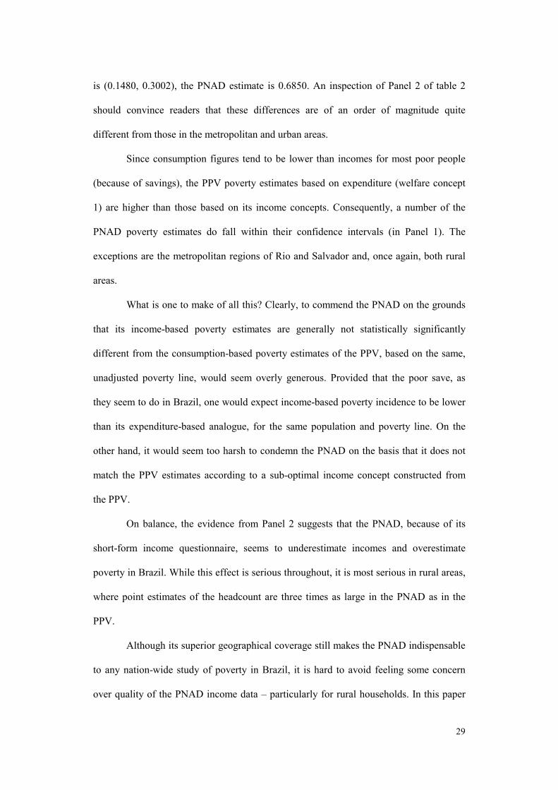
Since consumption figures tend to be lower than incomes for most poor people
(because of savings), the PPV poverty estimates based on expenditure (welfare concept
1) are higher than those based on its income concepts. Consequently, a number of the
PNAD poverty estimates do fall within their confidence intervals (in Panel 1). The
exceptions are the metropolitan regions of Rio and Salvador and, once again, both rural
areas.
What is one to make of all this? Clearly, to commend the PNAD on the grounds
that its income-based poverty estimates are generally not statistically significantly
different from the consumption-based poverty estimates of the PPV, based on the same,
unadjusted poverty line, would seem overly generous. Provided that the poor save, as
they seem to do in Brazil, one would expect income-based poverty incidence to be lower
than its expenditure-based analogue, for the same population and poverty line. On the
other hand, it would seem too harsh to condemn the PNAD on the basis that it does not
match the PPV estimates according to a sub-optimal income concept constructed from
the PPV.
On balance, the evidence from Panel 2 suggests that the PNAD, because of its
short-form income questionnaire, seems to underestimate incomes and overestimate
poverty in Brazil. While this effect is serious throughout, it is most serious in rural areas,
where point estimates of the headcount are three times as large in the PNAD as in the
PPV.
Although its superior geographical coverage still makes the PNAD indispensable
to any nation-wide study of poverty in Brazil, it is hard to avoid feeling some concern
over quality of the PNAD income data – particularly for rural households. In this paper
30
we have focused on urban areas, and on ordinal comparisons of profiles, rather than on
the absolute values of poverty measures. The reader is nevertheless cautioned that all
rural poverty measures discussed above are likely to be substantial overestimates, and
that even urban measures are likelier to be above than below the true mark.
In future, two alternative paths can be followed to deal with this situation. In the
medium-run, pending a thorough review of Brazil’s household survey system, one could
use innovative statistical procedures to combine data-sets, seeking to complement their
strengths and compensate for their weaknesses. Such techniques, although still in their
infancy, usually rely on imputing key variables from small but detailed data sets to larger
ones where they are either absent of measured with unacceptable margins of error. See
Hentschel et. al. (1999) and Elbers et. al. (1999). The other alternative is probably first-
best, if cost constraints are not binding: that is to redesign the survey system so as to
replace various sub-optimal instruments with a single well-designed survey.
6.CONCLUSIONS
The first conclusion of this study is that all the other conclusions must be treated
with circumspection, since they are based on a data set which seems likely to
systematically underestimate non-labor incomes, particularly for self-employed earners
and principally in rural areas.
The second main conclusion is that poverty in Brazil, subject to the foregoing
caveat, remains substantial. Even after adding imputed rents to the PNAD data, and
deflating prices regionally, the national average incidence of indigence in 1996,
measured with respect to a food-only poverty line, was 23%. Using a conceptually
preferable poverty line, which allows for expenditure on some non-food items (according
to the actual consumption patterns of those people whose incomes are equal to the food
poverty line), we find a poverty incidence of 45%.
31
Based on our data, poverty remains more acute in rural areas (headcounts of 52%
for the indigence line and 78% for the main poverty line) than in urban areas (headcounts
of 15% for the indigence line, and 37% for the main poverty line).24 However, since only
21% of Brazilians live in rural areas, the urban shares in the composition of poverty are
higher: 52% of people living below the indigence line live in urban areas, as do 64% of
those with incomes lower than the main poverty line.
Interestingly, urban poverty varies considerably with the type of urban
environment. Small cities (population < 20,000) have a higher poverty incidence than
medium-sized ones (20,000 – 100,000), and these have a higher incidence than large
cities (population > 100,000). The cores of metropolitan areas are least poor, but their
peripheries have higher headcounts. Small cities and metropolitan areas have the highest
poverty shares among urban environments, each accounting for roughly 18-19% of the
national total, but metropolitan areas account for a smaller share of the indigent (13.5%).
Greater research on and policy initiatives aimed at reducing poverty in small and medium
urban areas would seem to be a priority, along with the continuing need to tackle rural
poverty.
Urban poverty, like total poverty, also varies markedly across regions, with the
Northeast and the North reporting higher poverty rates than the Southeast or the South,
according to all three indices used. However, the higher population share of the
Southeast causes it and the Northeast to have the largest numbers of poor people in the
country. All this information on spatial variations suggests that there is considerable
scope for a finer geographical targeting of government poverty-reduction programs.
Poverty and living standards maps have been constructed for Brazil down to the
24 Overall urban headcounts refer to all non-rural areas, and are computed straight-forwardly from the information in Table 7.
32
municipality level (see UNDP, 1998), and it would be interesting to compare the
allocation of social spending by federal and state governments with those maps.
Our analysis also indicates that families are likelier to be poor if they are larger,
and particularly if they have larger numbers of children. Among the characteristics of the
household head, the main determinant of a household’s vulnerability to poverty is his or
her level of education, with (national) poverty rates declining from 75% for those with
one year of schooling or less, to 2% for those with more than 12 years. Race and age are
also important (unconditional) correlates of poverty, which is higher among households
headed by blacks, and lowest among those headed by Asians. Poverty incidence declines
monotonically with the age of the head.
The poor are less likely to rent or pay mortgages on their houses than to own
them outright, but their houses are generally of worse quality, and they enjoy
disproportionately low rates of access to services like piped water, electricity, garbage
collection or phone lines. The implications for future public spending on these types of
infrastructure should be obvious: using the information on the geographical location of
groups without access to these services, which can be quite detailed, expansions should
be targeted to them.
Poverty is high among the unemployed and informal sector workers, whether the
latter are self-employed or unregistered employees (‘sem carteira’). However, a greater
share of the poor is in self-employment than in any other labor status category. There is a
continuing need to ensure that adequate safety nets are in place, to protect not only
formal employees who lose their jobs and may have access to time-bound unemployment
benefits, but also to cushion the effect of falling aggregate demand and demand for labor
on informal employees and on the self-employed.
All things considered, there are perhaps two main conclusions from this exercise.
The first is that the Brazilian household survey system can be substantially improved at

33
little or no extra cost, so as to provide much more reliable information on living
standards across this vast country. The second is that, notwithstanding the above, there is
sufficient information in this poverty profile to guide a reallocation of crucial social
spending on education, health and social protection, to ensure a more effective use of
public resources in helping the poorest people in Brazil.
34
REFERENCES
AMADEO, E., J.M. CAMARGO, G. GONZAGA, R. PAES DE BARROS AND R. MENDONCA (1994): “A Natureza e o Funcionamento do Mercado de Trabalho Brasileiro desde 1980”, IPEA Discussion Paper No. 353, Rio de Janeiro. BOURGUIGNON, F., F.H.G. FERREIRA AND P.G. LEITE (2002): "Beyond Oaxaca-Blinder: Accounting for Differences in Household Income Distributions", mimeo, PUC-Rio. BUHMANN, B., L. RAINWATER, G. SCHMAUS AND T. SMEEDING (1988): “Equivalence Scales, Well-being, Inequality and Poverty: Sensitivity Estimates Across Ten Countries using the Luxembourg Income Study Database”, Review of Income and Wealth, 34, pp.115-142. COULTER, F.A.E., F.A. COWELL AND S.P. JENKINS (1992): “Equivalence Scale Relativities and the Extent of Inequality and Poverty”, Economic Journal, 102, pp.1067-1082. DEATON, A.S. (1989): “Looking for Boy-Girl Discrimination in Household Expenditure Data”, World Bank Economic Review, 3, pp.1-15. DEATON, A.S. (1997): The Analysis of Household Surveys: Microeconometric Analysis for Development Policy, (Baltimore: The Johns Hopkins University Press). ELBERS, C., J.O. LANJOUW AND P. LANJOUW (1999): “Welfare in Villages and Towns: Micro-Measurement of Poverty and Inequality”, mimeo, Free University of Amsterdam. FERREIRA, F.H.G., P. LANJOUW AND M. NERI (2000): "A New Poverty Profile for Brazil using PPV, PNAD and Census Data", Texto para Discussão No. 418, PUC-Rio . FERREIRA, F.H.G. AND J.A. LITCHFIELD (1996): “Growing Apart: Inequality and Poverty Trends in Brazil in the 1980s”, LSE – STICERD – DARP Discussion Paper No.23, London (August). FERREIRA, F.H.G. AND J.A. LITCHFIELD (2001): "Education or Inflation?: The Micro and Macroeconomics of the Brazilian Income Distribution During 1981-1995", Cuadernos de Economia, 38, pp.209-238. FOSTER, J.E., J. GREER AND E. THORBECKE (1984): “A Class of Decomposable Poverty Indices”, Econometrica, 52, pp.761-766. HARRIS, J.R. AND TODARO, M. (1970): “Migration, Unemployment and Development”, American Economic Review, 60, pp.126-142.
35
HENTSCHEL, J., J. O. LANJOUW, P. LANJOUW AND J. POGGI (forthcoming), “Combining Census and Survey Data to Study Spatial Dimensions of Poverty: A Case Study of Ecuador”, World Bank Economic Review (forthcoming). HOFFMAN, R. (2001): "Desigualdade no Brasil: A Contribuição das Aposentadorias", UNICAMP, Instituto de Economia, mimeo. LANJOUW, P. AND J.O. LANJOUW (1996): “Poverty Comparisons with Non-Compatible Data: Theory and Illustrations”, Yale University, Department of Economics, mimeo, (August). LANJOUW, P. AND M. RAVALLION (1995), “Poverty and Household Size”, Economic Journal, 105, pp.433. NERI, M. "Aspectos Fiscais e Sociais de Modalidades Alternativas de Reajuste de Aposentadorias e Pensões Públicas", em Coleção Previdência Social: Previdência, Assistência Social e Combate à Pobreza / Série Debates, Vol. 03, Brasília, 2001. NERI, M. et all. “Gasto Público en Servicios Sociales Básicos en Brasil” em Gasto Público en Servicios Sociales Básicos en América Latina y el Caribe: Análisis desde la perspectiva de la Iniciativa 20/20, organizado por Enrique Ganuza, Arturo Leon e Pablo Sauma, Mundiprensa, Santiago, 1999. NERI, M and CAMARGO, J. M. “Distributive Effects of Brazilian Structural Reforms” em Brazil in the 1990s: A Decade in Transition, organizado por Renato Baumann, Palgrave - Macmillan's Global Academic Publishing, UK, 2002. QUISUMBING, A.R., L. HADDAD AND C. PENA (1995): “Gender and Poverty: New Evidence from Ten Developing Countries”, IFPRI – FCND Discussion Paper No.9, Washington, DC, (December). RAVALLION, M. AND B. BIDANI (1994): “How Robust is a Poverty Profile?”, World Bank Economic Review, 8 (1), pp.75-102. ROCHA, S. (1993): “Poverty Lines for Brazil: New Estimates from Recent Empirical Evidence”, IPEA, Rio de Janeiro, mimeo. UNDP (1998): Relatório Sobre o Desenvolvimento Humano no Brasil, 1998. (Brasília: IPEA and UNDP). WORLD BANK (1998): “Public Expenditures for Poverty Alleviation in Northeast Brazil: Promoting Growth and Improving Services”, World Bank LAC Report.
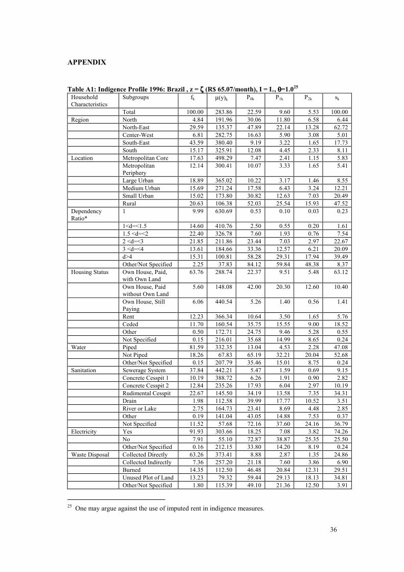
36
APPENDIX
Table A1: Indigence Profile 1996: Brazil , z = ζζζζ (R$ 65.07/month), I = I+, θθθθ=1.025
Household Characteristics
Subgroups fk µ(y)k P0k P1k P2k sk
Total 100.00 283.86 22.59 9.60 5.53 100.00 Region North 4.84 191.96 30.06 11.80 6.58 6.44 North-East 29.59 135.37 47.89 22.14 13.28 62.72 Center-West 6.81 282.75 16.63 5.90 3.08 5.01 South-East 43.59 380.40 9.19 3.22 1.65 17.73 South 15.17 325.91 12.08 4.45 2.33 8.11 Location Metropolitan Core 17.63 498.29 7.47 2.41 1.15 5.83 Metropolitan
Periphery 12.14 300.41 10.07 3.33 1.65 5.41
Large Urban 18.89 365.02 10.22 3.17 1.46 8.55 Medium Urban 15.69 271.24 17.58 6.43 3.24 12.21 Small Urban 15.02 173.80 30.82 12.63 7.03 20.49 Rural 20.63 106.38 52.03 25.54 15.93 47.52 Dependency Ratio*
1 9.99 630.69 0.53 0.10 0.03 0.23
1<d=<1.5 14.60 410.76 2.50 0.55 0.20 1.61 1.5 <d=<2 22.40 326.78 7.60 1.93 0.76 7.54 2 <d=<3 21.85 211.86 23.44 7.03 2.97 22.67 3 <d=<4 13.61 184.66 33.36 12.57 6.21 20.09 d>4 15.31 100.81 58.28 29.31 17.94 39.49 Other/Not Specified 2.25 37.83 84.12 59.84 48.38 8.37 Housing Status Own House, Paid,
with Own Land 63.76 288.74 22.37 9.51 5.48 63.12
Own House, Paid without Own Land
5.60 148.08 42.00 20.30 12.60 10.40
Own House, Still Paying
6.06 440.54 5.26 1.40 0.56 1.41
Rent 12.23 366.34 10.64 3.50 1.65 5.76 Ceded 11.70 160.54 35.75 15.55 9.00 18.52 Other 0.50 172.71 24.75 9.46 5.28 0.55 Not Specified 0.15 216.01 35.68 14.99 8.65 0.24 Water Piped 81.59 332.35 13.04 4.53 2.28 47.08 Not Piped 18.26 67.83 65.19 32.21 20.04 52.68 Other/Not Specified 0.15 207.79 35.46 15.01 8.75 0.24 Sanitation Sewerage System 37.84 442.21 5.47 1.59 0.69 9.15 Concrete Cesspit 1 10.19 388.72 6.26 1.91 0.90 2.82 Concrete Cesspit 2 12.84 235.26 17.93 6.04 2.97 10.19 Rudimental Cesspit 22.67 145.50 34.19 13.58 7.35 34.31 Drain 1.98 112.58 39.99 17.77 10.52 3.51 River or Lake 2.75 164.73 23.41 8.69 4.48 2.85 Other 0.19 141.04 43.05 14.88 7.53 0.37 Not Specified 11.52 57.68 72.16 37.60 24.16 36.79 Electricity Yes 91.93 303.66 18.25 7.08 3.82 74.26 No 7.91 55.10 72.87 38.87 25.35 25.50 Other/Not Specified 0.16 212.15 33.80 14.20 8.19 0.24 Waste Disposal Collected Directly 63.26 373.41 8.88 2.87 1.35 24.86 Collected Indirectly 7.36 257.20 21.18 7.60 3.86 6.90 Burned 14.35 112.50 46.48 20.84 12.31 29.51 Unused Plot of Land 13.23 79.32 59.44 29.13 18.13 34.81 Other/Not Specified 1.80 115.39 49.10 21.36 12.50 3.91
25 One may argue against the use of imputed rent in indigence measures.
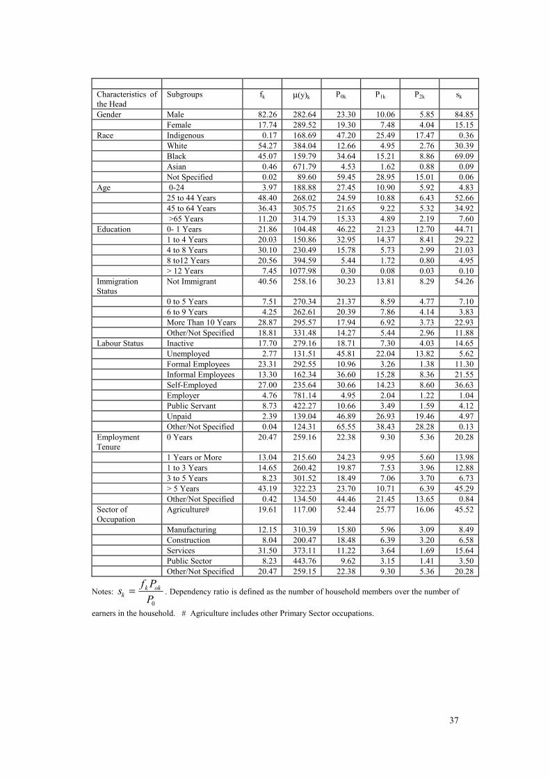
37
Characteristics of the Head
Subgroups fk µ(y)k P0k P1k P2k sk
Gender Male 82.26 282.64 23.30 10.06 5.85 84.85 Female 17.74 289.52 19.30 7.48 4.04 15.15 Race Indigenous 0.17 168.69 47.20 25.49 17.47 0.36 White 54.27 384.04 12.66 4.95 2.76 30.39 Black 45.07 159.79 34.64 15.21 8.86 69.09 Asian 0.46 671.79 4.53 1.62 0.88 0.09 Not Specified 0.02 89.60 59.45 28.95 15.01 0.06 Age 0-24 3.97 188.88 27.45 10.90 5.92 4.83 25 to 44 Years 48.40 268.02 24.59 10.88 6.43 52.66 45 to 64 Years 36.43 305.75 21.65 9.22 5.32 34.92 >65 Years 11.20 314.79 15.33 4.89 2.19 7.60 Education 0- 1 Years 21.86 104.48 46.22 21.23 12.70 44.71 1 to 4 Years 20.03 150.86 32.95 14.37 8.41 29.22 4 to 8 Years 30.10 230.49 15.78 5.73 2.99 21.03 8 to12 Years 20.56 394.59 5.44 1.72 0.80 4.95 > 12 Years 7.45 1077.98 0.30 0.08 0.03 0.10 Immigration Status
Not Immigrant 40.56 258.16 30.23 13.81 8.29 54.26
0 to 5 Years 7.51 270.34 21.37 8.59 4.77 7.10 6 to 9 Years 4.25 262.61 20.39 7.86 4.14 3.83 More Than 10 Years 28.87 295.57 17.94 6.92 3.73 22.93 Other/Not Specified 18.81 331.48 14.27 5.44 2.96 11.88 Labour Status Inactive 17.70 279.16 18.71 7.30 4.03 14.65 Unemployed 2.77 131.51 45.81 22.04 13.82 5.62 Formal Employees 23.31 292.55 10.96 3.26 1.38 11.30 Informal Employees 13.30 162.34 36.60 15.28 8.36 21.55 Self-Employed 27.00 235.64 30.66 14.23 8.60 36.63 Employer 4.76 781.14 4.95 2.04 1.22 1.04 Public Servant 8.73 422.27 10.66 3.49 1.59 4.12 Unpaid 2.39 139.04 46.89 26.93 19.46 4.97 Other/Not Specified 0.04 124.31 65.55 38.43 28.28 0.13 Employment Tenure
0 Years 20.47 259.16 22.38 9.30 5.36 20.28
1 Years or More 13.04 215.60 24.23 9.95 5.60 13.98 1 to 3 Years 14.65 260.42 19.87 7.53 3.96 12.88 3 to 5 Years 8.23 301.52 18.49 7.06 3.70 6.73 > 5 Years 43.19 322.23 23.70 10.71 6.39 45.29 Other/Not Specified 0.42 134.50 44.46 21.45 13.65 0.84 Sector of Occupation
Agriculture# 19.61 117.00 52.44 25.77 16.06 45.52
Manufacturing 12.15 310.39 15.80 5.96 3.09 8.49 Construction 8.04 200.47 18.48 6.39 3.20 6.58 Services 31.50 373.11 11.22 3.64 1.69 15.64 Public Sector 8.23 443.76 9.62 3.15 1.41 3.50 Other/Not Specified 20.47 259.15 22.38 9.30 5.36 20.28
Notes: s f PPk
k ok=0
. Dependency ratio is defined as the number of household members over the number of
earners in the household. # Agriculture includes other Primary Sector occupations.