UNICAMPrepositorio.unicamp.br/bitstream/REPOSIP/308817/1/Vidal...Vidal, Edison Iglesias de Oliveira...
192
i UNICAMP ASPECTOS EPIDEMIOLÓGICOS DAS FRATURAS DO FÊMUR PROXIMAL EM IDOSOS Tese de Doutorado Faculdade de Ciências Médicas Departamento de Medicina Preventiva e Social Aluno: Edison Iglesias de Oliveira Vidal Orientador: Prof. Dr. Djalma de Carvalho Moreira Filho CAMPINAS 2010
Transcript of UNICAMPrepositorio.unicamp.br/bitstream/REPOSIP/308817/1/Vidal...Vidal, Edison Iglesias de Oliveira...
i
UNICAMP
ASPECTOS EPIDEMIOLÓGICOS DAS FRATURAS DO FÊMUR PROXIMAL EM IDOSOS
Tese de Doutorado
Faculdade de Ciências Médicas Departamento de Medicina Preventiva e Social
Aluno: Edison Iglesias de Oliveira Vidal
Orientador: Prof. Dr. Djalma de Carvalho Moreira Filho
CAMPINAS
2010

iii
Edison Iglesias de Oliveira Vidal
ASPECTOS EPIDEMIOLÓGICOS DAS FRATURAS DO FÊMUR PROXIMAL EM IDOSOS
Tese apresentada à Pós-graduação da Faculdade de Ciências Médicas da Universidade Estadual de Campinas para obtenção do título de Doutor em Saúde Coletiva, área de concentração em Epidemiologia.
Orientador: Prof. Dr. Djalma de Carvalho Moreira Filho
CAMPINAS
iv
FICHA CATALOGRÁFICA ELABORADA PELA BIBLIOTECA DA FACULDADE DE CIÊNCIAS MÉDICAS DA UNICAMP
Bibliotecário: Sandra Lúcia Pereira – CRB-8ª / 6044
Título em inglês : Epidemiological aspects of hip fractures in the elderly Keywords: Hip fracture Osteoporosis Epidemiology Elderly Mortality Titulação: Doutor em Saúde Coletiva Área de concentração: Epidemiologia Banca examinadora: Profº. Drº. Djalma de Carvalho Moreira Filho Profª. Drª. Marília de Sá Carvalho Profº. Drº. Paulo José Fortes Villas Boas Profº. Drº. Carlos Roberto Silveira Correa Profº. Drº. João Batista de Miranda Data da defesa: 10-07-2010
Vidal, Edison Iglesias de Oliveira V667a Aspectos epidemiológicos das fraturas do fêmur proximal em
idosos / Edison Iglesias de Oliveira Vidal. Campinas, SP : [s.n.], 2010.
Orientador : Djalma de Carvalho Moreira Filho Tese ( Doutorado ) Universidade Estadual de Campinas. Faculdade
de Ciências Médicas. 1. Fraturas do quadril. 2. Osteoporose. 3. Epidemiologia. 4.
Idoso. 5. Mortalidade. I. Moreira Filho, Djalma de Carvalho. II. Universidade Estadual de Campinas. Faculdade de Ciências Médicas. III. Título.

v
vii
Dedico este trabalho aos meus pais,
Com quem primeiro aprendi;
Ao amor com que me criaram;
À Fernanda, amada, companheira e eterna namorada,
E à Julia que neste momento encontra-se em viagem
Do Céu para a Terra, para alegrar nossas vidas,
Aprendendo, ensinando, amando e sendo amada!

ix
Agradecimentos:
Ao Prof. Dr. Djalma de Carvalho Moreira Filho, pela amizade, pelos conselhos e pela confiança.
À Prof. Dra. Cláudia Medina Coeli, que primeiro me apresentou à epidemiologia e segue sempre iluminando meu caminho.
Aos Profs. Drs. Kenneth Rochel Camargo Jr., Rejane Sobrinho Pinheiro e Liz Maria de Almeida, com quem iniciei ainda na graduação e também em companhia da profa. Cláudia as primeiras pesquisas sobre a epidemiologia dos idosos com fraturas do fêmur proximal.
Ao Prof. Dr. Régis Blais, cuja parceria viabilizou parte importante deste trabalho.
Aos amigos do Serviço de Assistência Domiciliar do Hospital Israelita Albert Einstein e do Serviço de Assistência e Internação Domiciliar das regiões Norte e Leste de Campinas, pela parceria, carinho, amizade e admiração mútuos.
Ao Dr. Otávio, Dra. Marli, à vó Mercedes e ao vô Eugênio, que com tanta ternura me acolheram em sua família.

xi
“Aqui chegamos ao ponto de que talvez devêssemos ter partido.
O do inacabamento do ser humano.
Na verdade, o inacabamento do ser ou sua inconclusão é próprio da experiência vital.
Onde há vida, há inacabamento.
Mas só entre mulheres e homens o inacabamento tornou-se consciente.”
“A consciência do mundo e a consciência de si como ser inacabado
necessariamente inscrevem o ser consciente de sua inconclusão
num permanente movimento de busca.”
“Gosto de ser gente porque, inacabado, sei que sou um ser condicionado mas,
consciente do inacabamento, sei que posso ir mais além dele.”
(Paulo Freire, em Pedagogia da Autonomia)
xiii
Resumo
As fraturas do fêmur proximal (FFP) correspondem a um importante problema de
saúde pública em todo o mundo. Dentre todas as fraturas associadas à osteoporose são
consideradas como as mais graves e correlacionam-se com os maiores índices de morbi-
mortalidade, dependência funcional e custos para os indivíduos e os sistemas de saúde. O
maior crescimento em sua incidência nos próximos anos é esperado nos países em
desenvolvimento, todavia, estes também são os locais onde é maior a carência por dados
acerca da epidemiologia dos pacientes acometidos por estas fraturas.
A presente pesquisa teve como objetivo analisar alguns aspectos desta
epidemiologia tanto no âmbito nacional como internacional. Como resultado foram
confeccionados três artigos abordando esta temática.
O primeiro artigo avaliou, a partir de uma base de dados de todas as hospitalizações
por FFP na província de Quebec, no Canadá, a hipótese da equivalência do intervalo de
tempo entre a fratura e a cirurgia e o intervalo entre a hospitalização e a cirurgia, enquanto
preditores da ocorrência de óbito intra-hospitalar. Após controle para a presença de outras
variáveis, nenhum dos intervalos mostrou associar-se com a mortalidade intra-hospitalar.
Concluiu-se que, ao menos na medida em que a diferença entre os intervalos sejam
pequenas como no caso obervado, os mesmos podem ser utilizados de modo intercambiável
sem comprometer a interpretação da associação entre o timing cirúrgico e a mortalidade
intra-hospitalar, tal como pressuposto em diversos estudos prévios da literatura
internacional.
xiv
O segundo artigo buscou caracterizar o perfil clínico de idosos brasileiros
hospitalizados em função de uma FFP, bem como os padrões de tratamento adotados, as
complicações intra-hospitalares e a mortalidade ao longo de um ano. Dentre outros
resultados de interesse, observou-se uma taxa de mortalidade em um ano de 13,4%
(IC95%: 10,1 – 17,5%) e intervalos bastante elevados tanto entre a fratura e a
hospitalização (média de 3,6 dias) como entre a internação e a cirurgia (média de 12,8
dias).
O terceiro artigo procurou avaliar dentro do contexto brasileiro a associação entre o
intervalo de tempo da fratura à cirurgia e a sobrevida dos idosos acomeditos por uma FFP.
Após ajuste para variáveis de confundimento observou-se uma associação entre uma maior
demora para a internação hospitalar e o óbito (HR: 1,08 , IC95%: 1,04 – 1,12, P < 0,001).
Discute-se a questão das FFP enquanto objeto epidemiológico privilegiado,
inclusive como um possível evento sentinela a ser monitorado no âmbito da saúde do idoso
tanto no plano nacional como internacional.
xv
Abstract
Hip Fractures (HF) represent the most severe of all osteoporotic fractures and
remain an important cause of mortality, morbidity, dependency and costs for older adults
and healthcare systems worldwide. Even though the greatest increase regarding the
incidence of HF is expected to occur in the developing countries of the World, those are
also the regions from where less information is available regarding the epidemiology of
those fractures.
The present research aimed to analyze selected aspects of the epidemiology of those
fractures both in Brazil and internationally. Three manuscripts were produced as a direct
result of this investigation.
The first manuscript assessed the widely adopted assumption of interchangeability
between the gap from hospital admission to surgical HF repair and the actual gap from
fracture to surgery as predictors of in-hospital mortality among HF patients. A database
encompassing all HF hospital admissions in Quebec, Canada, was the primary source of
data for the analyses undertaken in this study. After statistical adjustment for the presence
of other covariates neither of the time intervals to surgery was a significant predictor of in
hospital mortality. As a conclusion, at least to the extent of the small differences observed
between both gaps, they might be used interchangeably without compromising the
interpretation of the relationship between surgical timing and in-hospital mortality, as
assumed by previous studies.
The second manuscript aimed to describe the clinical profile, treatment patterns, in-
hospital complications and one-year mortality of elderly Brazilians with an incident HF.
xvi
Among other findings 13.4% (95%CI: 10.1% – 17.5%) of patients died during the first year
and large gaps from fracture to hospital admission (mean 3.6 days) and from hospital
admission to surgery (mean 12.8 days) were noted.
The third manuscript examined in the context of a developing country the
association between surgical timing and the survival of older adults after a HF. After
adjusting for the presence of other covariates a small association between delayed hospital
admission and reduced survival (HR: 1.08, 95% CI: 1.04 – 1.12) was observed.
The point is made that HF should be considered a privileged epidemiological object,
which might be used strategically as a sentinel event to be monitored both locally and
internationally as a marker of the quality of health care to the elderly.
17
Sumário
RESUMO...............................................................................................................................................XIII ABSTRACT............................................................................................................................................ XV INTRODUÇÃO GERAL.......................................................................................................................... 21
INCIDÊNCIA, PREVALÊNCIA E PROJEÇÕES................................................................................................. 21 MORBIDADE E MORTALIDADE ................................................................................................................. 28 IMPACTO FINANCEIRO ............................................................................................................................. 33 FFP ENQUANTO OBJETO EPIDEMIOLÓGICO PRIVILEGIADO ......................................................................... 36
OBJETIVOS............................................................................................................................................. 39 CAPÍTULO 1: HIP FRACTURE IN THE ELDERLY: DOES COUNTING TIME FROM FRACTURE TO SURGERY OR FROM HOSPITAL ADMISSION TO SURGERY MATTER WHEN STUDYING IN-HOSPITAL MORTALITY?....................................................................................................................... 41
ABSTRACT .............................................................................................................................................. 42 INTRODUCTION ....................................................................................................................................... 43 MATERIALS AND METHODS ..................................................................................................................... 45 RESULTS................................................................................................................................................. 47 DISCUSSION ............................................................................................................................................ 50 CONCLUSION .......................................................................................................................................... 53 REFERENCES........................................................................................................................................... 54
CAPÍTULO 2: CLINICAL PROFILE OF ELDERLY BRAZILIANS WITH HIP FRACTURE: COMORBIDITIES, TREATMENT PATTERNS, COMPLICATIONS AND MORTALITY...................... 61
ABSTRACT .............................................................................................................................................. 62 INTRODUCTION ....................................................................................................................................... 63 METHODS ............................................................................................................................................... 64 RESULTS.............................................................................................................................................. 65 DISCUSSION ............................................................................................................................................ 65 CONCLUSION .......................................................................................................................................... 68 REFERENCES........................................................................................................................................... 76
CAPÍTULO 3: THE TIMING OF SURGERY FACTOR FOR OLDER ADULTS WITH HIP FRACTURES IN A DEVELOPING COUNTRY.................................................................................... 81
ABSTRACT .............................................................................................................................................. 82 INTRODUCTION ....................................................................................................................................... 83 METHODS ............................................................................................................................................... 84 RESULTS................................................................................................................................................. 86 DISCUSSION ............................................................................................................................................ 87 CONCLUSION .......................................................................................................................................... 90 FIGURES AND TABLES ............................................................................................................................. 91 REFERENCES........................................................................................................................................... 95
DISCUSSÃO GERAL .............................................................................................................................. 99 FFP ENQUANTO EVENTO SENTINELA PARA A ATENÇÃO À SAÚDE DO IDOSO .............................................. 100

19
CONCLUSÃO GERAL.......................................................................................................................... 105 REFERÊNCIAS ..................................................................................................................................... 107 ANEXO 1: GRÁFICOS DE RESÍDUOS DE SCHOENFELD.............................................................. 115 ANEXO 2: SCRIPT DE PROGRAMAÇÃO UTILIZADO................................................................... 143 ANEXO 3: COPYRIGHT ...................................................................................................................... 205
21
Introdução Geral
O tema das fraturas do fêmur proximal (FFP), também denominadas de fraturas de
quadril (FQ), em idosos possui grande relevância para a Saúde Coletiva não apenas no
Brasil, mas em todo o globo. Sua importância decorre das altas taxas de mortalidade e
dependência funcional associadas a estes tipos de fraturas; dos grandes montantes de
recursos financeiros gastos direta e indiretamente com o cuidado prestado a estes pacientes;
bem como de sua crescente incidência em inúmeros países em função do envelhecimento
populacional.
Incidência, Prevalência e Projeções
Estima-se que no início da década de 90 do século passado ocorriam a cada ano
cerca de 1,3 milhão de novas FQ no mundo (1, 2). Estima-se que no ano de 1990 havia no
mundo cerca de 4,48 milhões de indivíduos convivendo com alguma limitação decorrente
de uma FFP (2). Gullberg et al (3) debruçaram-se sobre a questão da projeção da incidência
das FFP no mundo até o ano de 2050. Neste estudo, os autores levaram em consideração
para seus cálculos as estimativas futuras de envelhecimento populacional disponíveis para
as diferentes regiões do globo, bem como um conjunto de cenários possíveis para a
tendência secular de incidência destas fraturas. Para a construção dos cenários relativos à
tendência secular, os autores tomaram por base estudos populacionais de diversos países,
nos quais em sua maioria foi observado um acréscimo na incidência anual padronizada por
idade e sexo para as FFP durante a segunda metade do século XX. Desta forma os autores
produziram um conjunto de cinco projeções para o total de FFP incidentes no mundo, com

22
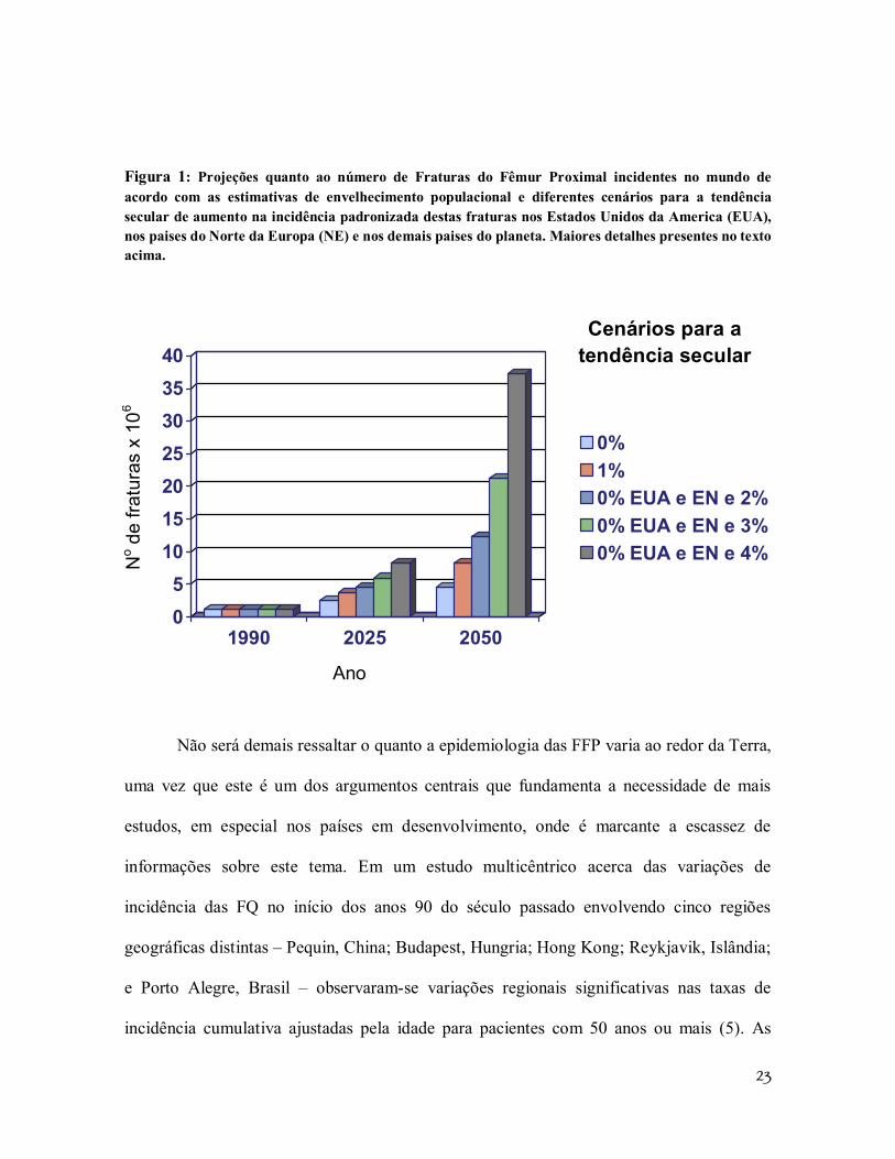
base em cinco possíveis cenários para a tendência secular (Figura 1). No primeiro cenário
examinaram o crescimento do total anual de FQ frente à perspectiva de uma tendência
secular de incremento nula. Nesta situação, portanto o aumento no número de FFP seria
atribuído exclusivamente ao fenômeno do envelhecimento populacional, de modo
semelhante à projeção realizada por Cooper, Campion e Melton III em 1992 (4). Para a
segunda projeção os autores assumiram uma tendência secular de incremento de um
porcento ao ano na incidência das FFP em todas as regiões geográficas. Já para os três
cenários subseqüentes de projeções, os autores assumiram por um lado uma tendência
secular nula para os EUA e para os países do norte da Europa – onde já havia relatos de
uma convergência para estabilidade da taxa anual de FQ – e por outro lado um aumento
anual de 2%, 3% e 4% para a incidência padronizada nos demais países (Figura 1).
Analisando estas diferentes estimativas os pesquisadores consideram que, com parcimônia,
deve-se esperar para o ano de 2050 algo entre 7,3 e 21,3 milhões de pacientes com FQ
incidentes no mundo. É importante notar que o maior incremento no número de pacientes
com FFP deverá ocorrer na Ásia, América Latina e África.
23
Figura 1: Projeções quanto ao número de Fraturas do Fêmur Proximal incidentes no mundo de acordo com as estimativas de envelhecimento populacional e diferentes cenários para a tendência secular de aumento na incidência padronizada destas fraturas nos Estados Unidos da America (EUA), nos paises do Norte da Europa (NE) e nos demais paises do planeta. Maiores detalhes presentes no texto acima.
05
10152025303540
1990 2025 2050
0%1%0% EUA e EN e 2%0% EUA e EN e 3%0% EUA e EN e 4%
Não será demais ressaltar o quanto a epidemiologia das FFP varia ao redor da Terra,
uma vez que este é um dos argumentos centrais que fundamenta a necessidade de mais
estudos, em especial nos países em desenvolvimento, onde é marcante a escassez de
informações sobre este tema. Em um estudo multicêntrico acerca das variações de
incidência das FQ no início dos anos 90 do século passado envolvendo cinco regiões
geográficas distintas – Pequin, China; Budapest, Hungria; Hong Kong; Reykjavik, Islândia;
e Porto Alegre, Brasil – observaram-se variações regionais significativas nas taxas de
incidência cumulativa ajustadas pela idade para pacientes com 50 anos ou mais (5). As
No d
e fra
tura
s x
106
Ano
Cenários para a tendência secular
24
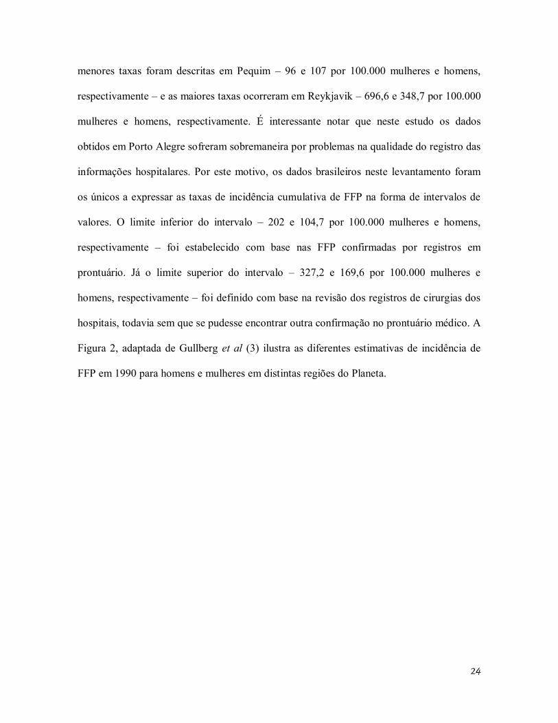
menores taxas foram descritas em Pequim – 96 e 107 por 100.000 mulheres e homens,
respectivamente – e as maiores taxas ocorreram em Reykjavik – 696,6 e 348,7 por 100.000
mulheres e homens, respectivamente. É interessante notar que neste estudo os dados
obtidos em Porto Alegre sofreram sobremaneira por problemas na qualidade do registro das
informações hospitalares. Por este motivo, os dados brasileiros neste levantamento foram
os únicos a expressar as taxas de incidência cumulativa de FFP na forma de intervalos de
valores. O limite inferior do intervalo – 202 e 104,7 por 100.000 mulheres e homens,
respectivamente – foi estabelecido com base nas FFP confirmadas por registros em
prontuário. Já o limite superior do intervalo – 327,2 e 169,6 por 100.000 mulheres e
homens, respectivamente – foi definido com base na revisão dos registros de cirurgias dos
hospitais, todavia sem que se pudesse encontrar outra confirmação no prontuário médico. A
Figura 2, adaptada de Gullberg et al (3) ilustra as diferentes estimativas de incidência de
FFP em 1990 para homens e mulheres em distintas regiões do Planeta.
25
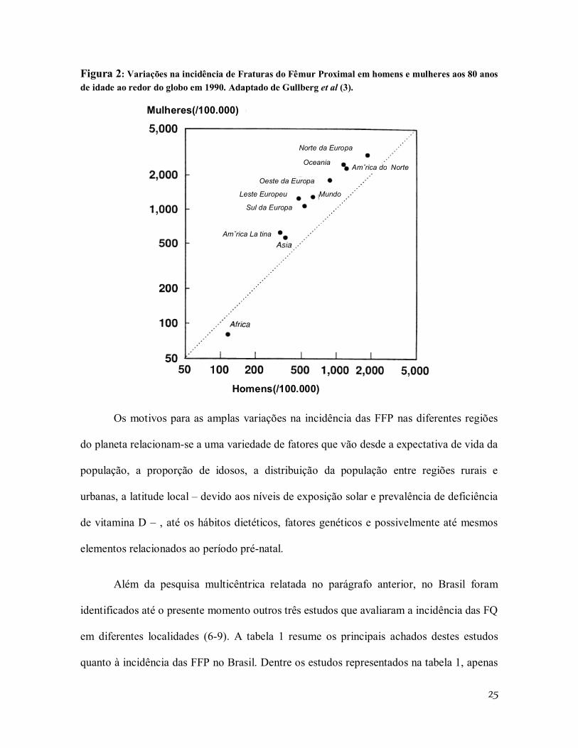
Figura 2: Variações na incidência de Fraturas do Fêmur Proximal em homens e mulheres aos 80 anos de idade ao redor do globo em 1990. Adaptado de Gullberg et al (3).
Mulheres(/100.000)
Homens(/100.000)
Norte da Europa
Amˇrica do Norte Oceania
Oeste da Europa
Leste Europeu
Sul da Europa
Mundo
Amˇrica La tina
Os motivos para as amplas variações na incidência das FFP nas diferentes regiões
do planeta relacionam-se a uma variedade de fatores que vão desde a expectativa de vida da
população, a proporção de idosos, a distribuição da população entre regiões rurais e
urbanas, a latitude local – devido aos níveis de exposição solar e prevalência de deficiência
de vitamina D – , até os hábitos dietéticos, fatores genéticos e possivelmente até mesmos
elementos relacionados ao período pré-natal.
Além da pesquisa multicêntrica relatada no parágrafo anterior, no Brasil foram
identificados até o presente momento outros três estudos que avaliaram a incidência das FQ
em diferentes localidades (6-9). A tabela 1 resume os principais achados destes estudos
quanto à incidência das FFP no Brasil. Dentre os estudos representados na tabela 1, apenas
26
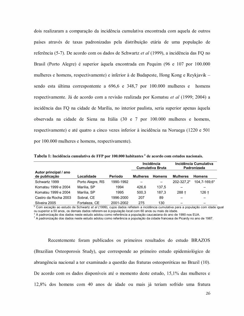
dois realizaram a comparação da incidência cumulativa encontrada com aquela de outros
países através de taxas padronizadas pela distribuição etária de uma população de
referência (5-7). De acordo com os dados de Schwartz et al (1999), a incidência das FQ no
Brasil (Porto Alegre) é superior àquela encontrada em Pequim (96 e 107 por 100.000
mulheres e homens, respectivamente) e inferior à de Budapeste, Hong Kong e Reykjavik –
sendo esta última correspontente a 696,6 e 348,7 por 100.000 mulheres e homens
respectivamente. Já de acordo com a revisão realizada por Komatsu et al (1999; 2004) a
incidência das FQ na cidade de Marília, no interior paulista, seria superior apenas àquela
observada na cidade de Siena na Itália (30 e 7 por 100.000 mulheres e homens,
respectivamente) e até quatro a cinco vezes inferior à incidência na Noruega (1220 e 501
por 100.000 mulheres e homens, respectivamente).
Tabela 1: Incidência cumulativa de FFP por 100.000 habitantes de acordo com estudos nacionais.
Incidência
Cumulativa Bruta Incidência Cumulativa
Padronizada Autor principal / ano de publicação Localidade Período Mulheres Homens Mulheres Homens Schwartz 1999 Porto Alegre, RS 1990-1992 – – 202-327,2* 104,7-169,6* Komatsu 1999 e 2004 Marília, SP 1994 426,6 137,5 – – Komatsu 1999 e 2004 Marília, SP 1995 500,3 187,3 288 † 126 † Castro da Rocha 2003 Sobral, CE 1996-2000 207 89 – – Silveira 2005 Fortaleza, CE 2001-2002 275 130 – –
Com exceção ao estudo de Schwartz et al (1999), cujos dados refletem a incidência cumulativa para a população com idade igual ou superior a 50 anos, os demais dados referem-se à população local com 60 anos ou mais de idade. * A padronização dos dados neste estudo adotou como referência a população caucasiana do ano de 1990 nos EUA. † A padronização dos dados neste estudo adotou como referência a população da cidade francesa de Picardy no ano de 1987.
Recentemente foram publicados os primeiros resultados do estudo BRAZOS
(Brazilian Osteoporosis Study), que corresponde ao primeiro estudo epidemiológico de
abrangência nacional a ter examinado a questão das fraturas osteoporóticas no Brazil (10).
De acordo com os dados disponíveis até o momento deste estudo, 15,1% das mulheres e
12,8% dos homens com 40 anos de idade ou mais já teriam sofrido uma fratura
27
osteoporótica. Deste total de fraturas 12% corresponderiam a FQ (10). Aplicando estas
estimativas à distribuição da população brasileira obtida através do censo demográfico
realizado pelo IBGE no ano 2000, calculamos uma prevalência de cerca de 779.000
indivíduos que tenham sofrido uma FQ osteoporótica ao longo da vida. Todavia, deve-se
ter em mente o fato de este número tratar-se forçosamente de uma subestimativa, como é
fácil concluir frente à alta taxa de mortalidade que acompanha os pacientes acometidos por
estas fraturas (11, 12).
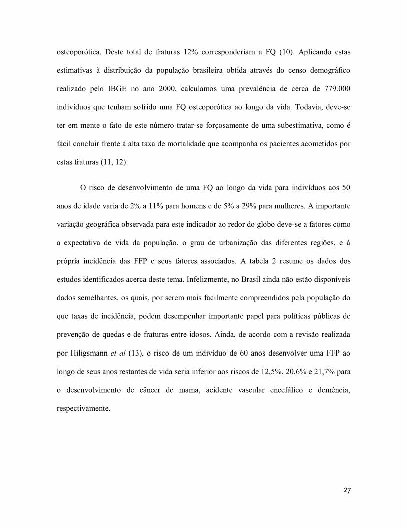
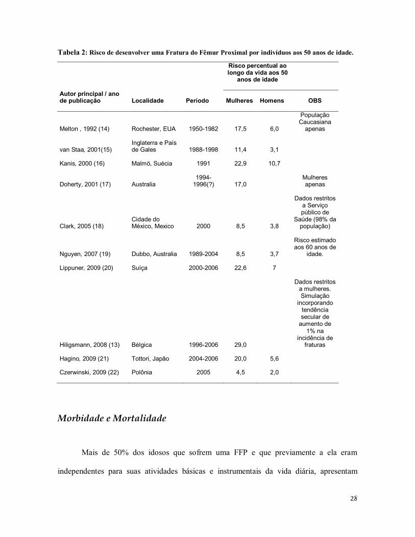
O risco de desenvolvimento de uma FQ ao longo da vida para indivíduos aos 50
anos de idade varia de 2% a 11% para homens e de 5% a 29% para mulheres. A importante
variação geográfica observada para este indicador ao redor do globo deve-se a fatores como
a expectativa de vida da população, o grau de urbanização das diferentes regiões, e à
própria incidência das FFP e seus fatores associados. A tabela 2 resume os dados dos
estudos identificados acerca deste tema. Infelizmente, no Brasil ainda não estão disponíveis
dados semelhantes, os quais, por serem mais facilmente compreendidos pela população do
que taxas de incidência, podem desempenhar importante papel para políticas públicas de
prevenção de quedas e de fraturas entre idosos. Ainda, de acordo com a revisão realizada
por Hiligsmann et al (13), o risco de um indivíduo de 60 anos desenvolver uma FFP ao
longo de seus anos restantes de vida seria inferior aos riscos de 12,5%, 20,6% e 21,7% para
o desenvolvimento de câncer de mama, acidente vascular encefálico e demência,
respectivamente.
28
Tabela 2: Risco de desenvolver uma Fratura do Fêmur Proximal por indivíduos aos 50 anos de idade.
Risco percentual ao longo da vida aos 50
anos de idade
Autor principal / ano de publicação Localidade Período Mulheres Homens OBS
Melton , 1992 (14) Rochester, EUA 1950-1982 17,5 6,0
População Caucasiana
apenas
van Staa, 2001(15) Inglaterra e País de Gales 1988-1998 11,4 3,1
Kanis, 2000 (16) Malmö, Suécia 1991 22,9 10,7
Doherty, 2001 (17) Australia 1994-
1996(?) 17,0 Mulheres apenas
Clark, 2005 (18) Cidade do México, Mexico 2000 8,5 3,8
Dados restritos a Serviço público de
Saúde (98% da população)
Nguyen, 2007 (19) Dubbo, Australia 1989-2004 8,5 3,7
Risco estimado aos 60 anos de
idade.
Lippuner, 2009 (20) Suíça 2000-2006 22,6 7
Hiligsmann, 2008 (13) Bélgica 1996-2006 29,0
Dados restritos a mulheres. Simulação
incorporando tendência secular de
aumento de 1% na
incidência de fraturas
Hagino, 2009 (21) Tottori, Japão 2004-2006 20,0 5,6
Czerwinski, 2009 (22) Polônia 2005 4,5 2,0
Morbidade e Mortalidade
Mais de 50% dos idosos que sofrem uma FFP e que previamente a ela eram
independentes para suas atividades básicas e instrumentais da vida diária, apresentam
29
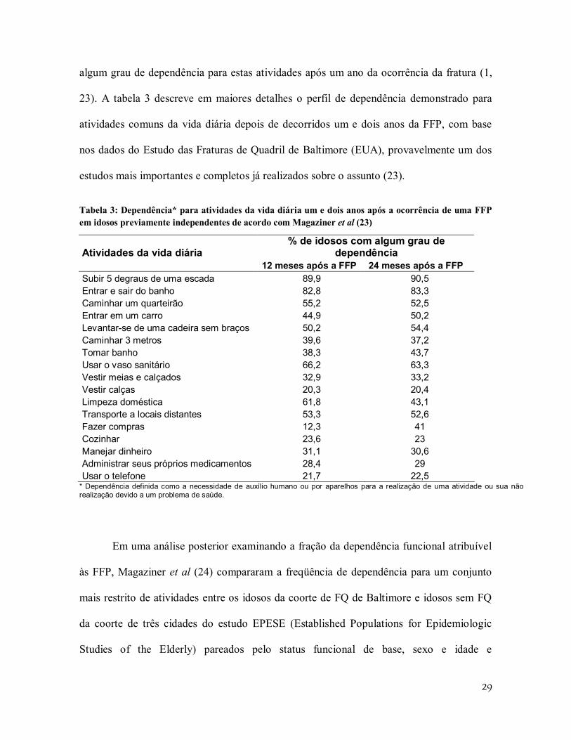
algum grau de dependência para estas atividades após um ano da ocorrência da fratura (1,
23). A tabela 3 descreve em maiores detalhes o perfil de dependência demonstrado para
atividades comuns da vida diária depois de decorridos um e dois anos da FFP, com base
nos dados do Estudo das Fraturas de Quadril de Baltimore (EUA), provavelmente um dos
estudos mais importantes e completos já realizados sobre o assunto (23).
Tabela 3: Dependência* para atividades da vida diária um e dois anos após a ocorrência de uma FFP em idosos previamente independentes de acordo com Magaziner et al (23)
Atividades da vida diária % de idosos com algum grau de
dependência 12 meses após a FFP 24 meses após a FFP Subir 5 degraus de uma escada 89,9 90,5 Entrar e sair do banho 82,8 83,3 Caminhar um quarteirão 55,2 52,5 Entrar em um carro 44,9 50,2 Levantar-se de uma cadeira sem braços 50,2 54,4 Caminhar 3 metros 39,6 37,2 Tomar banho 38,3 43,7 Usar o vaso sanitário 66,2 63,3 Vestir meias e calçados 32,9 33,2 Vestir calças 20,3 20,4 Limpeza doméstica 61,8 43,1 Transporte a locais distantes 53,3 52,6 Fazer compras 12,3 41 Cozinhar 23,6 23 Manejar dinheiro 31,1 30,6 Administrar seus próprios medicamentos 28,4 29 Usar o telefone 21,7 22,5
* Dependência definida como a necessidade de auxílio humano ou por aparelhos para a realização de uma atividade ou sua não realização devido a um problema de saúde.
Em uma análise posterior examinando a fração da dependência funcional atribuível
às FFP, Magaziner et al (24) compararam a freqüência de dependência para um conjunto
mais restrito de atividades entre os idosos da coorte de FQ de Baltimore e idosos sem FQ
da coorte de três cidades do estudo EPESE (Established Populations for Epidemiologic
Studies of the Elderly) pareados pelo status funcional de base, sexo e idade e
30
acompanhados por um período de dois anos. Os autores demonstraram que para cada 100
pacientes que haviam sofrido uma FQ, após dois anos de seguimento observava-se,
respectivamente, um excesso de 26 e 22 casos de dependência para deambular e realizar
transferência (ex. da cama para uma cadeira) em relação ao que poderia ser esperado do
processo de envelhecimento usual para o restante da população.
Outro dado que contribui para uma melhor noção do comprometimento funcional ao
qual os idosos com uma FFP recente estão expostos provém de um interessante estudo
israelense, onde se comparou o comprometimento funcional durante um programa de
reabilitação geriátrico entre portadores de uma FQ e pacientes acometidos por um acidente
vascular cerebral (25). Os autores constataram graus semelhantes de dependência funcional,
mensurada através da escala FIM (Functional Independence Measure), para os portadores
de AVC e FQ tanto no momento da admissão à unidade de reabilitação geriátrica como no
momento da alta.
Até o presente momento, o único estudo brasileiro prospectivo a avaliar o desfecho
funcional de idosos portadores de uma FFP observou que, depois de decorridos seis meses
do momento da fratura, apenas 30% dos sobreviventes haviam recuperado o mesmo grau de
desempenho funcional ulterior à mesma (26). Neste período cerca de 12% dos pacientes
tornaram-se totalmente dependentes e 9,3% foram institucionalizados.
Uma abordagem proposta pela Organização Mundial de Saúde para a quantificação
da carga (burden) à saúde decorrente de uma determinada condição patológica consiste na
determinação da medida de Anos de Vida Ajustados por Incapacidade (AVAI) – do ingês:
Disability Adjusted Life-Years (DALYs) (27). Trata-se de um indicador que incorpora os
31
anos de vida perdidos (AVP) bem como os anos de vida com incapacidade (AVI)
decorrentes da doença1. De modo geral, considera-se que um AVAI corresponde a um ano
de vida “saudável” perdido em função de determinada patologia. Johnel e Kanis (2)
procuraram quantificar o impacto da osteoporose no mundo através da estimação para o
ano de 1990 do número total de óbitos, dos anos de vida perdidos e dos anos de vida
ajustados por incapacidade decorrentes das FFP. Estes autores estimaram um total de
738.116 mortes, 1,2 milhão de anos de vida incapacitados, 1,7 milhão de anos de vida
perdidos e 2,9 milhão de anos de vida ajustados por incapacidade.
Os coeficientes de letalidade ao fim do primeiro ano após uma FQ apresentam
grande amplitude de variação, desde 5 a 67% (26, 28-41). No entanto a maior parte dos
estudos situa a letalidade entre 10 e 35% no primeiro ano após a fratura. Com o objetivo de
contextualizar melhor a dimensão da magnitude da letalidade subseqüente a uma FQ pode-
se citar que ela muitas vezes supera a letalidade da insuficiência cardíaca crônica (42),
outra condição grave e bastante comum nas faixas etárias mais avançadas. O coeficiente de
letalidade geral de idosos portadores de insuficiência cardíaca (classes funcionais II a IV da
New York Heart Association) situa-se ao redor de 13%. Para os idosos com insuficiência
cardíaca com classes funcionais II, III e IV a letalidade em um ano corresponde a cerca de
7%, 15% e 28%, respectivamente (42).
1 AVAI = AVP + AVI. Por sua vez, AVP corresponde número total de óbitos multiplicado pela expectativa de vida ajustada para a idade na qual ocorreu o óbito. E o AVI é calculado a partir do número de casos incidentes da doença, multiplicado por um peso atribuído à incapacidade dela decorrente em uma escala de 0 (saúde perfeita) a 1 (óbito), e por uma média da duração estimada da incapacidade até a remissão ou óbito. No caso das estimativas citadas, a duração média da incapacidade decorrente de uma FFP e o peso a ela atribuído foi de 9,6 anos e 0,272, respectivamente (2).
32
No Brasil se tem notícia de apenas três estudos que avaliaram a mortalidade de
pacientes idosos após uma FFP. Fortes et al (26) encontraram na cidade de São Paulo para
56 idosos atendidos em dois hospitais universitários, nos anos de 2004 e 2005 um
coeficiente de letalidade de 23,2% nos primeiros seis meses após a fratura. Outros
pesquisadores encontraram na mesma cidade no ano de 2000, para um total de 56 pacientes
atendidos em um hospital universitário devido a uma FFP um total de 30% de óbitos após
um ano (41) . Vidal et al (28) observaram entre 606 idosos hospitalizados pelo SUS devido
a uma FFP na cidade do Rio de Janeiro no ano de 1995 um total de 21,5% de óbitos em um
ano. Neste último estudo o excesso de óbitos, representado pela razão de mortalidade
padronizada, foi superior em 980% quando comparado ao coeficiente de mortalidade geral
para população da mesma faixa etária e sexo, nos primeiros 30 dias após a hospitalização.
Se por um lado pode-se afirmar haver consenso quanto ao fato de que as FQ são
associadas a importante excesso de mortalidade nos primeiros meses após a fratura, o
mesmo não pode ser ratificado quando se discute a questão do excesso de mortalidade após
6 meses do evento traumático inicial. Recente revisão sistemática procurou examinar esta
questão e realizou uma meta-análise de 24 estudos prospectivos que compararam a
sobrevida de idosos após uma FQ com a da população geral ajustada por sexo e idade (43).
De acordo com os dados deste estudo, o excesso de mortalidade associado às FFP pode ser
observado até 10 anos após a fratura. Mulheres caucasianas que sofreram uma FQ aos 80
anos de idade demonstraram taxas de mortalidade anuais em excesso às mulheres da
mesma faixa etária na ordem de 8%, 11%, 18% e 22% em um, dois, cinco e 10 anos após a
fratura, respectivamente. Já para homens caucasianos acometidos por uma FFP aos 80 anos,
o excesso de mortalidade observado foi de 18%, 22%, 26% e 20% em um, dois, cinco e 10
33
anos após a fratura, respectivamente. A razão de risco – Hazard Ratio (HR) – observada
variou respectivamente para mulheres e homens de 5,75 e 7,95 três meses após a fratura a
1,96 e 1,79 depois de decorridos 10 anos. Como esperado, os maiores índices de letalidade
foram constatados imediatamente após a fratura. Logo em seguida constata-se uma
diminuição progressiva do risco de óbito até que este se torna relativamente constante a
partir do segundo ano após a fratura, embora permaneça o excesso de mortalidade em
relação àquele da população geral (43).
Impacto financeiro
Os custos decorrentes de uma FFP possuem grande impacto direto sobre os sistemas
de saúde, sobre os indivíduos acometidos e suas famílias. Muito embora uma revisão
exaustiva sobre os aspectos econômicos das FQ extrapole os objetivos e limites desta breve
introdução ao tema, entende-se ser fundamental a abordagem deste tópico para a
contextualização geral do assunto.
Os custos associados às FFP variam significativamente ao redor do mundo em
função tanto de aspectos locais – ex: incidência de FFP, padrões locais de recursos e custos
de cuidados hospitalares e de reabilitação – como por questões metodológicas associadas à
sua estimativa em diferentes estudos – ex: dados restritos a gastos diretos hospitalares
versus dados que incorporam custos indiretos familiares para a contratação de cuidadores
ou abandono de atividades remuneradas por familiares para cuidar do paciente após a alta
hospitalar.
Para o ano de 1995 nos EUA, Ray et al (44) estimaram um total de US$ 13,8
bilhões gastos de forma direta para os cuidados hospitalares e de reabilitação associados a
34
fraturas osteoporóticas. Deste total, as FQ seriam responsáveis por US$ 8,68 bilhões
(63,1%) e a maior parte de seus custos diretos corresponderiam às hospitalizações (64,2%
ou US$ 5,6 bilhões). Bass et al (45) investigando os gastos diretos do sistema de saúde
norte-americano devidos a uma FFP em veteranos idosos entre 1999 e 2003 encontraram
um gasto médio de US$ 69.389,00 por paciente durante o primeiro ano após a fratura,
sendo que 71,4% destes gastos ocorriam durante os primeiros 30 dias. Braithwaite et al (46)
realizaram simulações estatísticas por modelos de Markov com base na literatura
norteamericana sobre FFP em idosos de modo a estimar os custos associados a uma FFP
para uma coorte hipotética de pacientes com 80 anos de idade. Nesta análise os autores
incluíram gastos tardios após a alta hospitalar, incluindo o uso de instituições de longa
permanência de idosos, assistência domiciliar formal e informal. Assim sendo, estimaram
um custo total de cerca de US$ 81.300,00 por pessoa para os gastos totais em vida
decorrentes diretamente de uma FFP. Deste total US$ 8.900 deviam-se à hospitalização
inicial, US$ 3.900 a hospitalizações subseqüentes, US$ 35.400 à utilização de instituições
de longa permanência de idosos e US$ 30.800 a gastos com assistência domiciliar. É
interessante notar que dentre os gastos referidos com assistência domiciliar no longo prazo,
80% representavam gastos informais, não reembolsáveis pelo seguro-saúde e
desempenhados por familiares ou amigos (46). De modo semelhante os custos estimados
para aquele pais para as fraturas originadas no ano de 1997 alcançariam a cifra de US$ 27
bilhões.
Na Suíça as fraturas osteoporóticas correspondem à primeira causa de
hospitalização ajustada pela idade entre as mulheres, ultrapassando as doenças
cardiovasculares, os cânceres de mama, os ginecológicos e a doença pulmonar obstrutiva
35
crônica (DPOC) (47). Naquele país, entre os homens, apenas as hospitalizações por DPOC
foram mais comuns que aquelas devido a fraturas osteoporóticas. De acordo com Lippumer
et al (47) o custo médio para a internação hospitalar associada a uma FQ foi de 18.227 e
16.941 francos suíços para cada mulher e homem hospitalizado respectivamente,
correspondento a uma duração média da internação de 19,1 e 17,9 dias.
Haentjens et al (48) conduziram na Bélgica entre 1995 e 1996 um interessante
estudo prospectivo comparando ao longo de um ano os gastos de saúde de 159 idosos
acometidos por uma FFP incidente com os gastos de idosos pareados por sexo, idade e
local de residência. O custo médio da hospitalização inicial foi de US$ 9.534 – variando de
de US$ 2.703 a 37.406 – , com um tempo médio de duração de internação de 29 dias. O
custo médio anual de gastos de saúde para os pacientes com uma FFP foi de US$ 13.470 e
de US$ 6.170 para os indivíduos do grupo controle, portanto, correspondendo a um excesso
médio de US$ 7.300 por indivíduo devido a uma FQ. É importante notar que este estudo
não incluiu gastos indiretos associados aos cuidados por familiares e amigos, nem gastos
diretos envolvendo medicamentos de uso extra-hospitalar, transporte de ambulância, ou
com serviços para cuidados domésticos.
Na América Latina investigadores da Organização Pan-americana de Saúde
estimaram em torno de US$ 5.500 o custo médio direto associado à uma hospitalização por
uma FQ no Brasil no ano 2000 (49). De acordo com Komatsu et al (6) na cidade de Marília,
no interior de São Paulo, no ano de 1995 o custo de uma hospitalização por uma FFP para o
SUS foi em média de US$ 1.733,77 por paciente, com uma duração média de internação de
12 dias. Já o custo direto associado a uma hospitalização devido a uma FQ no Sistema
Suplementar de Saúde Brasileiro entre 2003 e 2004 nos estados de Minas Gerais, São Paulo
36
e Rio de Janeiro, foi estimado em cerca de R$ 24.000 (aproximadamente US$ 8.300 ao
câmbio da época de US$ 1 = R$ 2,90), com uma duração média de internação de 9.2 dias,
dos quais 2,1 dias teriam ocorrido em uma Unidade de Terapia Intensiva (50). Do valor
total gasto na hospitalização pelo Sistema Suplementar de Saúde Brasileiro, cerca de 61%
seriam relativos a materiais, em especial às próteses de quadril (51).
FFP enquanto objeto epidemiológico privilegiado
Além dos elementos descritos acima que corroboraram a questão da relevância das
FFP tanto no plano individual como coletivo, estas fraturas apresentam algumas
particularidades que fazem delas um objeto privilegiado para o estudo epidemiológico.
Primeiramente pode-se dizer que seu processo diagnóstico é razoavelmente mais simples e
direto que aquele associado a diversas patologias comuns à população idosa2. Trata-se
eminentemente de uma condição altamente sintomática, marcada por dor e
comprometimento agudo da capacidade de deambular. Seu tratamento de primeira linha é
cirúrgico, de forma que a quase totalidade das FFP é referenciada a hospitais, o que as torna
mais facilmente rastreáveis através de sistemas de informação hospitalar. São associadas no
2 ‡A título de exemplo: o diagnóstico das diferentes síndromes demenciais requer muitas vezes a realização de testes neuropsicológicos, uma variedade de exames laboratoriais e de imagem e, sobretudo, um montante importante de julgamento clínico sujeito a grande variabilidade entre profissionais. O mesmo se dá com o processo diagnóstico de insuficiência cardíaca, das tonturas e de várias outras condições patológicas comuns entre os idosos. Por outro lado, o diagnóstico da maioria absoluta das FFP se dá de modo razoavelmente direto através da observação de radiografias simples do segmento afetado, sendo bastante infreqüentes as situações em que se faz necessária a solicitação de Ressonância Magnética Nuclear ou Cintilografia óssea.
37
curto e médio prazo com outro tipo de desfecho já rotineiramente monitorado por sistemas
de informação em saúde presentes na maioria dos países: o óbito. Estas características,
fizeram com que as FFP fossem denominadas de “barômetro internacional da osteoporose”
(38) e tenham sido utilizadas como marcador primário da carga desta doença no mundo em
diversas pesquisas (1, 2). Ainda, o estudo da epidemiologia das FFP se presta a análises
sobre todo o ciclo de atenção à saúde do idoso desde a prevenção primária de quedas e
tratamento da osteoporose até a reabilitação posterior dos pacientes e prevenção de novas
fraturas.
Tendo em vista os argumentos expostos acima bem como a grande amplitude do
tema, optou-se por abordar ao longo dos capítulos subseqüentes alguns aspectos da
epidemiologia das FFP em idosos.
39
Objetivos
Capitulo 1: O objetivo deste estudo foi o de verificar uma suposição adotada
amplamente na literatura sobre as FFP em idosos: a hipótese da equivalência do intervalo
de tempo entre a fratura e a cirurgia e o intervalo entre a hospitalização e a cirurgia,
enquanto preditores da ocorrência de óbito intra-hospitalar.
Capítulo 2: Este estudo objetivou caracterizar o perfil clínico de idosos brasileiros
hospitalizados em função de uma FFP, bem como os padrões de tratamento adotados, as
complicações intra-hospitalares e a sobrevivência ao longo de um ano.
Capítulo 3: Este estudo almejou avaliar dentro do contexto brasileiro a associação
do intervalo de tempo entre a fratura e cirurgia e a sobrevivência dos idosos acomeditos por
uma FFP.
41
Capítulo 1: Hip fracture in the elderly: does counting time from fracture to surgery or from hospital admission to surgery matter when studying in-hospital mortality?
Publicado em Osteoporos Int (2009) 20:723–729 DOI 10.1007/s00198-008-0757-1
Disponível em http://www.springerlink.com/content/b53n674vh5358v72/
E. I. O. Vidal1, 2, D. C. Moreira-Filho1, C. M. Coeli3, K. R. Camargo Jr.4, F. B. Fukushima5
and R. Blais6
Received: 7 June 2008 / Accepted: 18 August 2008 / Published online: 7 October 2008
# International Osteoporosis Foundation and National Osteoporosis Foundation 2008
(1) Social and Preventive Medicine Department, State University of Campinas, Campinas,
SP, Brazil
(2) Home Care Department, Albert Einstein Hospital, Av. Albert Einstein 627/701, 10th
floor, São Paulo, SP, Brazil
(3) Institute of Studies on Public Health, Federal University of Rio de Janeiro, Rio de
Janeiro, RJ, Brazil
(4) Social Medicine Institute, State University of Rio de Janeiro, Rio de Janeiro, RJ, Brazil
(5) Anesthesiology Department, State University of São Paulo, Botucatu, SP, Brazil
(6) Health Administration Department, University of Montreal, Montreal, QC, Canada
42
Abstract
Summary This study aims to analyze whether the interval from hospital admission to
surgery may be used as a surrogate of the actual gap from fracture to surgery when
investigating in-hospital hip fracture mortality. After analyzing 3,754 hip fracture
admissions, we concluded that those intervals might be used interchangeably without
misinterpretation bias.
Introduction The debate regarding the influence of time to surgery in hip fracture (HF)
mortality is one of the most controversial issues in the HF medical literature. Most previous
investigations actually analyzed the time from hospital admission to surgery as a surrogate
of the less easily available gap from fracture to surgery. Notwithstanding, the assumption of
equivalency between those intervals remains untested.
Methods We analyzed 3,754 hospital admissions of elderly patients due to HF in Quebec,
Canada. We compared the performance as predictors of in-hospital mortality of the delay
from admission to surgery and the actual gap from fracture to surgery using univariate and
multiple logistic regression analysis.
Results The mean times from fracture to surgery and from admission to surgery were 1.84
and 1.02 days (P<0.001), respectively. On univariate logistic regression, both times were
slightly significant as mortality predictors, yielding similar odds ratios of 1.08 (P<0.001)
for time from fracture to surgery and 1.11 (P<0.001) for time from admission to surgery.
43
After accounting for other covariates, neither times remained significant mortality
predictors.
Conclusion The gap from admission to surgery may be used as a surrogate of the actual
delay from fracture to surgery when studying in-hospital HF mortality.
Keywords: Elderly. Hip fracture . Mortality . Osteoporosis . Time to surgery
Introduction
Hip fractures (HF) are considered the most severe of the osteoporotic fractures and
are associated with great impact on morbidity, mortality, and costs for the elderly
population and healthcare systems. The role of the delay between the HF and its surgical
treatment on post-HF mortality of elderly patients is certainly one of the most controversial
issues on HF epidemiology in the medical literature [1–5]. The reasons for this controversy
rely on several factors, namely, (1) the diverging results found by the different groups
examining this issue using different methodologies [1, 3, 6–11], (2) the ethical impediment
of designing a randomized controlled trial purposefully delaying the time of the surgical
procedure [3–5, 11, 12], and (3) the difficulty in determining the extent to which the
mortality rates observed are a function of the actual delay to surgery or of the burden of
comorbidities and clinical instability of elderly patients with HF [1, 3, 7, 8, 12].
Even though the measure of time is one of the central concerns when investigating
this question, most studies have analyzed the time from hospital admission to surgery as a
surrogate for the most biologically relevant time gap from fracture to surgical repair [3],
44
relying on the assumption that any difference between those time intervals should be minor
or irrelevant. However, this assumption has not been previously verified, and there are
arguments to question its validity [13]. Orosz et al. [14], specifically analyzing the reasons
for delay in the hospitalization and surgical treatment of elderly patients with hip fractures,
found 17% of patients presenting to the hospital 24 h or more after the injury, which led to
the fracture. Still surprising is the finding that among those patients with delays of 24 h or
more from fracture to hospitalization, 48% presented to the hospital 72 h or later. Other
researchers [15] also observed 8% of HF patients being admitted to the hospital later than 2
days after the fracture, and Dolk [16] reported 14.6% of HF patients with delays before
arrival at the hospital, even though for that study the amount of delay was not clearly
specified.
If significant proportions of HF patients are admitted to the hospital with
unexpected delays from the time of fracture, it would be reasonable to question whether
previous studies investigating the association between time to surgery and HF mortality
could have suffered from a misclassification bias important enough to raise doubt about
their conclusions (e.g., patients with long delays from injury to surgery could have been
classified as patients with short delays from admission to surgery, and the true association
between time to surgery and HF mortality could have been concealed). Therefore, a
retrospective observational population-based cohort study was conducted to test the
currently used assumption that when investigating the influence of delays to surgery on in-
hospital mortality of elderly patients with osteoporotic HF, the time interval from hospital
admission to surgery might be used as a valid surrogate measure to the time from
fracture/injury to hospitalization.
45
Materials and methods
Data source The MED-ECHO database, which is the information system that encompasses all
hospital admissions in the province of Quebec, Canada, was the main source of data for this
study. It is a governmental database system with high standards of internal validity of
records and often used as data source in other epidemiological investigations [17, 18]. All
records of elderly aged 60 and older fulfilling the subsequent inclusion criteria were
identified: (a) Main hospital admission diagnosis was HF (as identified by the first three
digits of the International Classification of Diseases, ninth revision, ICD-9, code 820); (b)
hospital discharge occurred between April 1st, 2003 and March 31st, 2004.
In order to minimize selection bias and confounding, the following exclusion
criteria were adopted: (a) patients with a diagnosis of malignant cancer, (b) patients with a
record of high intensity trauma as the injury mechanism, (c) patients with open HF, (d)
patients without record of the time of the injury/fracture, (e) patients not undergoing a
surgical HF repair procedure, (f) patients whose fracture occurred before April 1st, 2003,
(g) patients whose interval between the fracture and hospital admission was above 10 days,
as it was assumed the chances would increase that the patient was indeed admitted due to a
complication of a previous fracture or miscoding of the date of injury.
Statistical analyses
Statistical analyses were performed using the R software version 2.6.2 [19]. We
analyzed the time intervals between fracture and hospital admission, fracture and surgery,
and hospital admission and surgery. The characteristics of patients regarding age, sex, type
46
of HF, place of origin prior to admission, number of diagnoses, and the Charlson
comorbidity index as adapted by D’Hoore et al. [17] were explored according to the time
interval between fracture and hospital admission. Patients were categorized under those
whose hospital admission occurred on the same day of the fracture, 1 to 2 days, and 3 days
or more thereafter. Comparisons between groups were made using analysis of Variance or
Chi-square test (χ2), according to the characteristics of the variable under examination. The
Charlson index [17] was calculated by means of the software CalcCharlson version 1.1 [20]
and was divided into four levels of progressive burden of comorbidity (0, 1, 2, and 3)
according to the first proposal by Charlson et al. [21].
Univariate and multiple logistic regression models were performed by examining
the relationships between inhospital mortality and a set of predictor variables, comprising
the previously mentioned time intervals, age, sex, type of HF, place of origin prior to
admission, number of diagnoses, the Charlson comorbidity index, type of surgical
procedure performed, type of anesthesia, and type of hospital where the surgical procedure
took place. The type of surgical procedure was categorized under (a) arthroplasty, (b)
internal fixation, or (c) other procedures. Types of anesthesia were analyzed as (a) regional
anesthesia, (b) general anesthesia, (c) a combination of general anesthesia and regional or
local anesthetic techniques, and (d) other techniques. Hospitals were described as (a)
hospitals with 100 beds of less, (b) hospitals with more than 100 beds, and (c) university
hospitals. The level of α for statistical significance was set at 0.05.
47
Results
Among the 3,754 patients who fulfilled the proposed criteria, there were 2,994
(79.8%) women. The mean age was 81.2 years (range 60–107), distributed as follows: 60 to
69 years old—301 (8%); 70–79 years old—1,024 (27.3%); 80–89 years old—1,741
(46.4%); 90 years old or older—688 (18.3%). The mean length of hospital stay was 27
days, with an interquartile range of 8 to 41 days. There were 342 deaths yielding a 9% in-
hospital mortality rate (95%CI 8.2–10%).
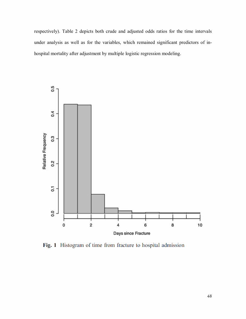
Nearly 44% of patients were admitted to the hospital on the same day of the injury
leading to the HF (group 1) and 51.2% during the first or second day after the fracture
(group 2), while 5% were admitted on the third day or later thereafter (group 3). Figure 1
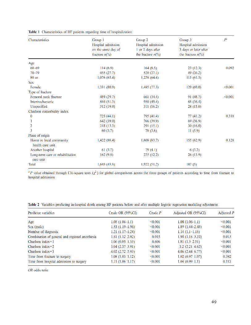
displays the relative distribution of time intervals from fracture to hospital admission. Table
1 depicts further details and comparisons regarding the characteristics of those three
groups.
The mean number of diagnosis among groups 1 through 3 were 6.9, 6.7 and 7.1
diagnoses (P=0.15), respectively. The mean times from fracture to surgery and from
admission to surgery were 1.84 and 1.02 days (P<0.001). On univariate logistic regression
analysis, the time intervals from fracture to surgery and from admission to surgery were
both significant predictors of in-hospital mortality, yielding the following respective odds
ratios of 1.08 (95% CI 1.03–1.12, P<0.001) and 1.11 (95%CI 0.1.06–1.17, P< 0.001).
However, after multiple logistic regression modeling with adjustment for the influence of
other covariates, both time intervals did not remain as significant predictors of in-hospital
mortality (OR:1.02, 95%CI 0.97–1.07, P= 0.392 and OR 1.04 95%CI 0.99–1.1, P=0.113,
48
respectively). Table 2 depicts both crude and adjusted odds ratios for the time intervals
under analysis as well as for the variables, which remained significant predictors of in-
hospital mortality after adjustment by multiple logistic regression modeling.
49
50
Discussion
Since the publication of Kenzora et al. [22] widely cited paper on HF mortality
more than 20 years ago, whose results directly challenged the long-established concept of
early surgery for HF, the debate on the influence of delays to surgery on HF associated
mortality has been one of the most controversial issues in the medical literature regarding
HF epidemiology and management. A total of 31 studies examining the relationship
between HF mortality and time to surgery were reviewed. Among those, 16 studies related
early surgery with lower mortality [3, 6–8, 10, 12, 23–32], 14 studies did not identify
significant mortality differences for patients undergoing early surgery [1, 2, 4, 5, 9, 11, 16,
33–39], and only one [22] found early surgery related to higher mortality rates. However,
major methodological differences among those studies make direct comparisons difficult, if
not impossible. The definition of early surgery itself varied considerably among researchers
analyzing time as a dichotomous variable. Many studies—mostly those where a protective
association was found between early surgery and mortality —did not manage to control for
confounding associated with comorbidity or functional status [7, 12, 16, 23, 24, 27, 28, 30,
31, 38], and Majumdar et al. [2], while analyzing their own data and considering the most
recent and rigorous studies on this issue [1, 36], concluded that any apparent difference in
mortality rates between early and later surgery was due to confounding related to
prefracture patient characteristics and surgical selection bias. Nevertheless, it seems that the
current debate on the effects of delays to HF surgical repair is far from an end, as a recently
published meta-analysis [40] of a set of 16 observational studies, in spite of much criticism
[41], concluded in favor of a protective effect regarding mortality for early surgical HF
repair.
51
The clinical reasoning behind the hypothesis of delayed HF surgical repair and
higher mortality is intimately related to the association of HF and restricted mobility [4, 31]
and the many negative physiological consequences of immobility for the elderly.
Notwithstanding, of all 31 analyzed studies examining the association between time to
surgical HF repair and mortality, only four of them [8, 25, 33, 38] actually analyzed the
time interval from fracture to surgery, as a more accurate marker of the period of restricted
mobility and therefore considered a biologically more relevant measure [3, 13]. The
remaining studies, either due to database limitations or to deliberate study design options,
restricted their analysis to the surrogate time from hospital admission to surgery or even
excluded patients with hospital admission beyond 48 h after the time of the fracture [1].
Such decisions rest on (a) choice to specifically study time from hospital admission to
surgery, as it could probably be the target of internal hospital logistical interventions; and
(b) the explicit or implicit assumption that any differences between time intervals from
fracture to surgery and from hospital admission to surgery should be minor or irrelevant [3,
42].
While investigating that assumption in the present study, we found that even though
a statistically significant difference could be traced between time from fracture to surgery
and from hospital admission to surgery (mean times 1.84 and 1.02 days, respectively,
P<0.001), the analysis of the relationship between those time intervals and inhospital
mortality was quite similar. Both time intervals at a first glance (univariate analysis)
displayed a small but statistically significant association with in-hospital mortality, which,
however, did not stand adjustment for the effect of other covariates including age, sex,
burden of comorbidity, and type of anesthesia among others (Table 2). The present results
52
suggest that the widely adopted assumption of equivalence of those time intervals regarding
mortality investigations is not unreasonable.
This study encompasses several limitations worth noting. First, the study design is
observational, which makes it more prone to bias than clinical trials [43]. Notwithstanding,
observational studies are the only alternative for issues such as the one examined here,
where ethical and logistical reasons make randomized clinical trials unfeasible [3, 11, 12]—
it would be unethical to randomize patients for later surgery, since unnecessary waiting is
likely to be associated with immobility, pain, and suffering for HF patients, and it would be
impossible to allocate patients to seeking hospital assistance earlier or later after a HF.
Second, it was not possible to control for other important variables unavailable in the
original database, such as nutritional, socioeconomic, mental and functional status prior to
the fracture, severity of the HF, rates of adoption of antithrombotic, and antibiotic
prophylaxis among other variables. Nevertheless, since the null hypothesis herein tested
already could not be rejected after adjustment for age, sex, comorbidity index, type of
anesthesia, and number of diagnosis, it would be unreasonable to believe that controlling
for the other unavailable variables would change the main result and lead to the rejection of
the hypothesis of no difference between considering time from hospital admission to
surgery and from fracture to surgery when examining in-hospital mortality.
As other authors [3, 5, 11, 26, 39] have done, we treated time as a discrete variable
measured in units of calendar days instead of the more accurate measure of hours since the
fracture. Notwithstanding, for orthopedic surgeons deciding upon the optimal timing of
surgical HF repair, counting time using calendar days as measurement units is a more
53
practical and clinically relevant criterion than the measure of hours since fracture or
hospital admission [11].
We also did not analyze deaths occurring after discharge of the first hospital
admission for HF. Therefore, the present results are intimately related to local practices
regarding hospital discharge [26], and it is known that in-hospital mortality analyses
usually underestimate even short-term mortality related to HF [44]. However, since
Canadian hospital discharge practices regarding HF are associated with significantly longer
hospital stays than in other countries such as the United States [26] and the observed mean
length of stay was 27 days (interquartile range from 8 to 41 days), it is believed that the
degree of short-term mortality underestimation should be minor.
Conclusion
This study is valuable for offering initial evidence that the often-adopted procedure
of using the time interval from hospital admission to surgery as a surrogate of the less
easily available time from fracture to surgery might indeed not be associated with
significant bias when analyzing inhospital mortality, at least as long as these are not too
different. Thereby, we give support to one of the assumptions of many previous and
possible future studies investigating this issue. In future research, it would be interesting to
determine if and at which “threshold” the difference in the two intervals leads to different
interpretations regarding the association of time to surgery and mortality. Further studies
are needed to understand the reasons, the consequences, and the profile of elderly HF
patients with large delays before hospital admission.
54
Acknowledgments We are grateful to Michèle Paré, analyst at the GRIS, University of
Montreal, for her assistance with the preparation of the MED-ECHO database. Three
authors (DCMF, CMC, and KRCJ) were partially supported by research fellowship grants
from the Brazilian National Council for Scientific and Technological Development
(CNPq). FBF was supported by a research fellowship grant from the State of São Paulo
Foundation for Research Support (FAPESP).
References
1. Grimes JP, Gregory PM, Noveck H, Butler MS, Carson JL (2002) The effects of
time-to-surgery on mortality and morbidity in patients following hip fracture. Am J
Med 112:702–709
2. Majumdar SR, Beaupre LA, Johnston DW, Dick DA, Cinats JG, Jiang HX (2006)
Lack of association between mortality and timing of surgical fixation in elderly
patients with hip fracture: results of a retrospective population-based cohort study.
Med Care 44:552–559
3. McGuire K, Bernstein J, Polsky D, Silber J (2004) Delays until surgery after hip
fracture increases mortality. Clin Orthop Rel Res 428:294–301
4. Rae HC, Harris IA, McEvoy L, Todorova T (2007) Delay to surgery and mortality
after hip fracture. ANZ J Surg 77:889–891
5. Novack V, Jotkowitz A, Etzion O, Porath A (2007) Does delay in surgery after hip
fracture lead to worse outcomes? A multicenter survey. Int J Qual Health Care
19:170–176
55
6. Bottle A, Aylin P (2006)Mortality associated with delay in operation after hip
fracture: observational study. BMJ 332:947–951
7. Doruk H, Mas MR, Yildiz C, Sonmez A, Kyrdemir V (2004) The effect of the
timing of hip fracture surgery on the activity of daily living and mortality in elderly.
Arch Gerontol Geriatr 39:179– 185
8. Gdalevich M, Cohen D, Yosef D, Tauber C (2004) Morbidity and mortality after
hip fracture: the impact of operative delay. Arch Orthop Trauma Surg 124:334–340
9. Moran CG, Wenn RT, Sikand M, Taylor AM (2005) Early mortality after hip
fracture: is delay before surgery important? J Bone Joint Surg Am 87:483–489
10. Weller I, Wai EK, Jaglal S, Kreder HJ (2005) The effect of hospital type and
surgical delay on mortality after surgery for hip fracture. J Bone Joint Surg Br
87:361–366
11. Zuckerman JD, Skovron ML, Koval KJ, Aharonoff G, Frankel VH (1995)
Postoperative complications and mortality associated with operative delay in older
patients who have a fracture of the hip. J Bone Joint Surg Am 77:1551–1556
12. Casaletto JA, Gatt R (2004) Post-operative mortality related to waiting time for hip
fracture surgery. Injury 35:114–120
13. Villar RN, Allen SM, Barnes SJ (1986) Hip fractures in healthy patients: operative
delay versus prognosis. Br Med J (Clin Res Ed) 293:1203–1204
14. Orosz GM, Hannan EL, Magaziner J, Koval K, Gilbert M, Aufses A, Straus E,
Vespe E, Siu AL (2002) Hip fracture in the older patient: reasons for delay in
hospitalization and timing of surgical repair. J Am Geriatr Soc 50:1336–1340
56
15. Hefley FG Jr., Nelson CL, Puskarich-May CL (1996) Effect of delayed admission
to the hospital on the preoperative prevalence of deep-vein thrombosis associated
with fractures about the hip. J Bone Joint Surg Am 78:581–583
16. Dolk T (1990) Operation in hip fracture patients—analysis of the time factor. Injury
21:369–372
17. D’Hoore W, Bouckaert A, Tilquin C (1996) Practical considerations on the use of
the Charlson comorbidity index with administrative data bases. J Clin Epidemiol
49:1429–1433
18. Levy AR, Tamblyn RM, Fitchett D, McLeod PJ, Hanley JA (1999) Coding
accuracy of hospital discharge data for elderly survivors of myocardial infarction.
Can J Cardiol 15:1277–1282
19. R Development Core Team (2008) R: A Language and Environment for Statistical
Computing. In. R Foundation for Statistical Computing, Vienna, Austria. Available
at: http://www.R-project.org
20. Camargo KR Jr., Coeli CM (2006) CalcCharlson v1.1. Available at
http://www.iesc.ufrj.br/reclink/. Accessed March 30, 2008
21. Charlson ME, Pompei P, Ales KL, MacKenzie CR (1987) A new method of
classifying prognostic comorbidity in longitudinal studies: development and
validation. J Chronic Dis 40:373–383
22. Kenzora JE, McCarthy RE, Lowell JD, Sledge CB (1984) Hip fracture mortality.
Relation to age, treatment, preoperative illness, time of surgery, and complications.
Clin Orthop Relat Res 186:45–56
23. Bredahl C, Nyholm B, Hindsholm KB, Mortensen JS, Olesen AS (1992) Mortality
after hip fracture: results of operation within 12 h of admission. Injury 23:83–86 24.
57
24. Davis FM, Woolner DF, Frampton C, Wilkinson A, Grant A, Harrison RT, Roberts
MT, Thadaka R (1987) Prospective, multi-centre trial of mortality following general
or spinal anaesthesia for hip fracture surgery in the elderly. Br J Anaesth 59:1080–
1088
25. Elliott J, Beringer T, Kee F, Marsh D, Willis C, Stevenson M (2003) Predicting
survival after treatment for fracture of the proximal femur and the effect of delays to
surgery. J Clin Epidemiol 56:788–795
26. Ho V, Hamilton BH, Roos LL (2000) Multiple approaches to assessing the effects
of delays for hip fracture patients in the United States and Canada. Health Serv Res
34:1499–1518
27. Perez JV, Warwick DJ, Case CP, Bannister GC (1995) Death after proximal
femoral fracture: an autopsy study. Injury 26:237–240
28. Todd CJ, Freeman CJ, Camilleri-Ferrante C, Palmer CR, Hyder A, Laxton CE,
Parker MJ, Payne BV, Rushton N (1995) Differences in mortality after fracture of
hip: the east Anglian audit. Bmj 310:904– 908
29. White BL, Fisher WD, Laurin CA (1987) Rate of mortality for elderly patients after
fracture of the hip in the 1980’s. J Bone JointSurg Am 69:1335–1340
30. Harty JA, McKenna P, Moloney D, D’Souza L, Masterson E (2007) Anti-platelet
agents and surgical delay in elderly patients with hip fractures. J Orthop Surg (Hong
Kong) 15:270–272
31. Rogers FB, Shackford SR, Keller MS (1995) Early fixation reduces morbidity and
mortality in elderly patients with hip fractures from low-impact falls. J Trauma
39:261–265
58
32. Hamlet WP, Lieberman JR, Freedman EL, Dorey FJ, Fletcher A, Johnson EE
(1997) Influence of health status and the timing of surgery onmortality in hip
fracture patients.AmJ Orthop 26:621–627
33. Davis TR, Sher JL, Porter BB, Checketts RG (1988) The timing of surgery for
intertrochanteric femoral fractures. Injury 19:244–246
34. Franzo A, Francescutti C, Simon G (2005) Risk factors correlated with post-
operative mortality for hip fracture surgery in the elderly: a population-based
approach. Eur J Epidemiol 20:985–991
35. Hoenig H, Rubenstein LV, Sloane R, Horner R, Kahn K (1997) What is the role of
timing in the surgical and rehabilitative care of community-dwelling older persons
with acute hip fracture? Arch Intern Med 157:513–520
36. Orosz GM, Magaziner J, Hannan EL, Morrison RS, Koval K, Gilbert M,
McLaughlin M, Halm EA, Wang JJ, Litke A, Silberzweig SB, Siu AL (2004)
Association of timing of surgery for hip fracture and patient outcomes. Jama
291:1738–1743
37. Stoddart J, Horne G, Devane P (2002) Influence of preoperative medical status and
delay to surgery on death following a hip fracture. ANZ J Surg 72:405–407
38. Parker MJ, Pryor GA (1992) The timing of surgery for proximal femoral fractures. J
Bone Joint Surg Br 74:203–205
39. Sund R, Liski A (2005) Quality effects of operative delay on mortality in hip
fracture treatment. Qual Saf Health Care 14:371–377
40. Shiga T, Wajima Z, Ohe Y (2008) Is operative delay associated with increased
mortality of hip fracture patients? Systematic review, meta-analysis, and meta-
regression: [Le delai operatoire est-il associe a une mortalite accrue chez les patients
59
atteints d’une fracture de la hanche ? Synthese systematique, meta-analyse et meta-
regression]. Can J Anaesth 55:146–154
41. Bryson GL (2008) Waiting for hip fracture repair—Do outcomes and patients
suffer?/En attendant une chirurgie pour fracture de la hanche: est-ce que les patients
et leur evolution en patissent? Can J Anaesth 55:135–139
42. Magaziner J, Simonsick EM, Kashner TM, Hebel JR, Kenzora JE (1989) Survival
experience of aged hip fracture patients. Am J Public Health 79:274–278
43. Bhandari M, Tornetta P 3rd, Ellis T, Audige L, Sprague S, Kuo JC, Swiontkowski
MF (2004) Hierarchy of evidence: differences in results between non-randomized
studies and randomized trials in patients with femoral neck fractures. Arch Orthop
Trauma Surg 124:10–16
44. Vidal EI, Coeli CM, Pinheiro RS, Camargo KR Jr. (2006) Mortality within 1 year
after hip fracture surgical repair in the elderly according to postoperative period: a
probabilistic record linkage study in Brazil. Osteoporos Int 17:1569–1576
61
Capítulo 2: Clinical Profile of Elderly Brazilians with Hip Fracture: comorbidities, treatment patterns, complications and mortality.
Vidal, EI 1,2,3; Moreira-Filho, DC2; Pinheiro, RS4; Souza, RC5; Almeida, LM6; Camargo Jr,
KR7; Coeli, CM4
Affiliations:
1- State University of São Paulo – UNESP 2- Sate University of Campinas – UNICAMP 3- Albert Einstein Hospital 4- Federal University of Rio de Janeiro – UFRJ 5- Serra dos Órgãos Foundation 6- National Câncer Institute – INCA 7- State University of Rio de Janeiro - UERJ
Corresponding author:
Edison Iglesias de Oliveira Vidal
e-mail: [email protected]
telephone: +55-11-34593007
Fax: +55-11-37470715
Conflict of interest: No disclosures.
62
Abstract
Introduction: There is a relative paucity of data encompassing the epidemiology of
Hip Fractures (HF) in the developing regions of the world. The present research aims to
describe the clinical profile, patterns of care and mortality rates of elderly HF patients at a
University Hospital responsible for a substantial share of all HF surgeries in Rio de Janeiro,
Brazil.
Methods: All medical records of patients aged 60 and older with a main admission
diagnosis of HF between 1995 and 2000 were reviewed. Mortality rates were determined
by means of Probabilistic Record Linkage Methodology linking the Hospital database with
the Brazilian Mortality Information System.
Results: Among 352 subjects, 74.4% were women and the mean age was 77.3
years. Most HF (54.8%) were of the intertrochanteric type. Internal fixation and hip
arthroplasties were performed in 64.1% and 35% of patients, respectively. The mean gaps
from fracture to hospital admission and from admission to surgery were 3.6 and 12.8 days,
respectively. Most patients (74%) underwent neuroaxial anesthesia. Less than 10% of
patients received in-hospital physiotherapy and almost 95% of patients underwent antibiotic
and deep venous thrombosis prophylaxis. Mortality rates 30 days, 90 days and one year
after the fracture were 3.4%, 8.0% and 13.4%, respectively.
Conclusion: Major delays from fracture to surgery and very low rates of in-hospital
physiotherapy are reported in the context of a developing country. Better understanding of
the clinical profile, patterns of care and outcomes of HF patients is vital for the design of
elder friendly public policies.
63
Keywords: Hip fracture, Osteoporosis, Epidemiology, Developing Countries, Brazil,
Elderly
Introduction
Hip Fractures (HF) are considered the most important osteoporotic fractures in
terms of clinical severity, disability and costs (1-3). Due to the fact that they are almost
always treated in hospitals and associated with pain and disability, they are less prone to
undernotification and therefore have been appointed as “an international barometer of
osteoporosis” (1). Around the Globe there is great variability concerning the incidence of
HF and its related mortality, which is explained as a consequence of diverse factors,
ranging from the interaction between different genotypes and environmental factors to
healthcare system organizational characteristics. Even though the greatest increase
regarding the incidence of HF is expected to occur in the developing countries of the
World, those are also the regions from where less information is available regarding the
epidemiology of those fractures (4). There is particularly few data concerning the clinical
profile of Brazilian and Latin American elderly with HF (5-9). Hence, the present research
was designed aiming to describe the comorbidity burden, the patterns of treatment, related
surgical and clinical complications, and mortality rates of elderly Brazilians with HF
admitted to a University Hospital responsible for a substantial share of all HF surgeries in
the city of Rio de Janeiro, a major metropolitan area in the Southeast of Brazil.
64
Methods
All medical records of patients aged 60 and older with a main admission diagnosis
of HF between 1995 and 2000 were reviewed and abstracted according to a standardized
instrument previously tested. Patients whose HF was related to a malignancy or who did
not undergo surgical repair were excluded.
In order to evaluate the one year mortality rates of the study patients, records were
linked to the database of the Brazilian Mortality Information System (MIS) from 1995 to
2001 by means of Probabilistic Record Linkage Methodology (PRLM) (6, 10-14). Previous
research in a similar setting revealed 85.5% sensitivity, 99.4% specificity, 98.1% and
94.9% positive and negative predictive values, respectively, regarding correct matching of
records between databases according to this methodological approach (15). The RecLink II
Software (16) was used for the implementation of PRLM followed by manual examination
of pairs of records with higher probability of representing a true match between databases.
Frequency tables were produced concerning the following variables: type of HF,
type of injury leading to HF, form of surgical treatment and anesthesia, time to surgery,
presence of venous thromboembolism and antibiotic prophylaxis, physiotherapy
rehabilitation during the episode of hospital admission, comorbidities as ascertained by the
Charlson Index (17) , American Society of Anesthesiology (ASA) physical status score,
clinical and surgical complications, length of stay, hospital readmission and mortality
during the first year after HF. Statistical analyses were performed using the R software
version 2.10.1 (18).
65
RESULTS
Among the 352 patients who fulfilled the proposed inclusion criteria, there were
262 (74.4%) women. The mean age overall was 77.3 years and women were mean 3.7
years older than men (mean ages 78.2 and 74.5 years, respectively; P = 0.001). The mean
length of stay was 20.5 days with an interquartile range of 14 to 24 days. The mean time
from the occurrence of the HF to hospital admission was 3.6 days (interquartile range 0-4
days) and the mean gap from hospital admission to surgery was 12.8 days (interquartile
range of 8-17 days). Figure 1 illustrates the distribution of time from hospital admission to
surgery. Figure 2 displays the one year Kaplan-Meier survival curve for this cohort of
patients. Table 1 depicts sociodemographic characteristics of the patients while Table 2
describes their clinical profile including number of comorbidities, types and causes of HF.
Table 3 portrays the frequency of surgical and anesthetic approaches adopted, as well of
standard clinical procedures such as antibiotic prophylaxis. Most femoral neck fractures
(82.7%) were managed by hip arthroplasties, while 92.8% of the intertrochanteric fractures
and 96.2% of the subtrochanteric fractures underwent internal fixation procedures. Table 4
represents the frequency of clinical and surgical complications during the hospital stay, one
year readmission and mortality rates.
Discussion
The large gaps observed from the occurrence of the fracture to hospital admission
and thereafter to surgery are remarkably different from those reported in developed
66
countries, where the vast majority of patients undergoes surgery during the first 48h of
hospital admission (19-24). Even when compared to data restricted to University hospitals,
where the gap from hospital admission to surgery is often larger – possibly due to selection
of patients with higher clinical complexity – the reported delays to surgery may be
considered quite large (22). Even more significant is the delay from fracture to hospital
admission, which might reflect issues ranging from problems in the access to appropriate
health care for elders with HF to the possibility of elder mistreatment. As previously cited
there is scarce information examining the magnitude of this gap, its causes and
consequences (19). Interestingly, the high rates of arthroplasty procedures for femoral neck
fractures might be related to the large gaps from fracture to surgery, since those gaps incur
in greater risk of avascular necrosis of the head of the femur.
Less than 10% of patients received in-hospital physiotherapy, which is significantly
divergent from current recommendations for early mobilization (25, 26) and again mirrors
limitations in the access to optimal healthcare resources. Nevertheless, almost 95% of
patients received deep venous thrombosis and antibiotic prophylaxis.
The majority of patients (74.1%) underwent neuroaxial anesthesia (i.e. spinal or
epidural), which represents a somewhat different pattern than that observed in many other
regions where general anesthesia usually represents a larger share of the anesthetic
procedures performed (27-29). The debate surrounding what type of anesthetic procedure is
best suited for HF patients does not seem to be resolved, notwithstanding, a recent
systematic review disclosed lower mortality at 30 days, lower incidence of deep vein
thrombosis and of postoperative mental confusion for HF patients undergoing neuroaxial
anesthesia, however no measurable long term differences in mortality were identified (30).
67
The one year mortality rate observed (13.4%) was much lower than the 21.5%
mortality rate described previously encompassing all public hospitals in the city of Rio de
Janeiro (6) and lies in the lower limits of mortality reported for HF around the world (1,2).
This might be due to several factors, as follows. First, University hospitals have been
shown to be associated with lower mortalities for HF than general hospitals even though
they often display larger gaps from hospital admission to surgery (22). It is not clear which
elements of the health care process in University hospitals are responsible for the lower
mortality, but it is possible that patients are assessed more often not only by medical
students and residents but also by experienced professors. Second, most patients in this
study were attributed a low Charlson comorbidity score and only roughly one third of
patients were considered to have a severe systemic disease according to the physical status
classification of the American Society of Anesthesiology. Third, the patient population was
relatively younger than usually reported by most studies from developed countries (22, 31,
32). Fourth, another possibility worth of consideration is that due to the large gaps from
fracture to hospital admission, frailer and acutely ill patients might not have been
transferred to the University Hospital, and therefore their deaths happened in other
institutions.
The present study encompasses several limitations worth noting. Since its design
was based on the standardized retrospective abstraction of medical records there were
several missing or unreadable data regarding some variables, as represented by the five
percent of patients with unspecified marital status, or the 21% and the almost three percent
of unspecified living arrangements and causes of the fracture, respectively.
Notwithstanding, the absence of those data may be regarded in itself as a reflection of the
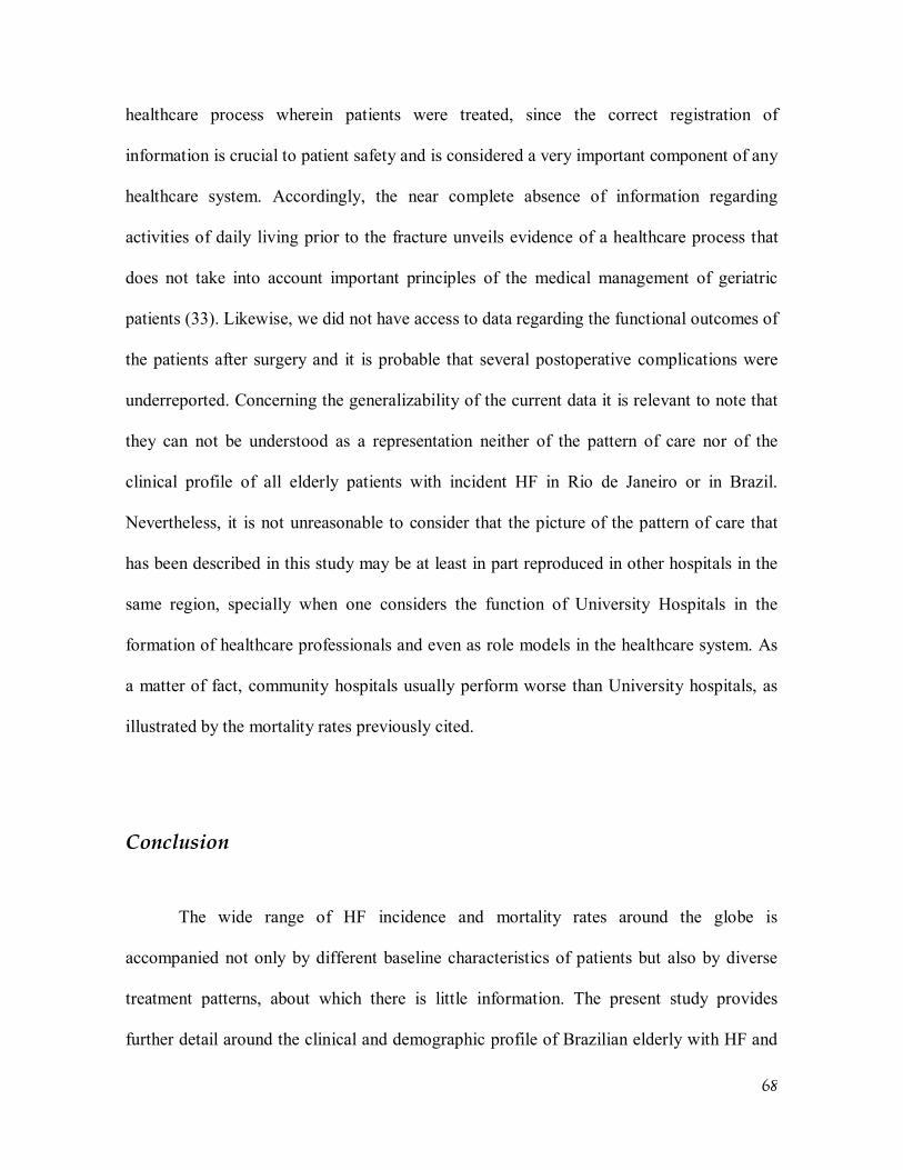
68
healthcare process wherein patients were treated, since the correct registration of
information is crucial to patient safety and is considered a very important component of any
healthcare system. Accordingly, the near complete absence of information regarding
activities of daily living prior to the fracture unveils evidence of a healthcare process that
does not take into account important principles of the medical management of geriatric
patients (33). Likewise, we did not have access to data regarding the functional outcomes of
the patients after surgery and it is probable that several postoperative complications were
underreported. Concerning the generalizability of the current data it is relevant to note that
they can not be understood as a representation neither of the pattern of care nor of the
clinical profile of all elderly patients with incident HF in Rio de Janeiro or in Brazil.
Nevertheless, it is not unreasonable to consider that the picture of the pattern of care that
has been described in this study may be at least in part reproduced in other hospitals in the
same region, specially when one considers the function of University Hospitals in the
formation of healthcare professionals and even as role models in the healthcare system. As
a matter of fact, community hospitals usually perform worse than University hospitals, as
illustrated by the mortality rates previously cited.
Conclusion
The wide range of HF incidence and mortality rates around the globe is
accompanied not only by different baseline characteristics of patients but also by diverse
treatment patterns, about which there is little information. The present study provides
further detail around the clinical and demographic profile of Brazilian elderly with HF and
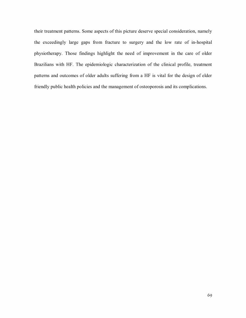
69
their treatment patterns. Some aspects of this picture deserve special consideration, namely
the exceedingly large gaps from fracture to surgery and the low rate of in-hospital
physiotherapy. Those findings highlight the need of improvement in the care of older
Brazilians with HF. The epidemiologic characterization of the clinical profile, treatment
patterns and outcomes of older adults suffering from a HF is vital for the design of elder
friendly public health policies and the management of osteoporosis and its complications.
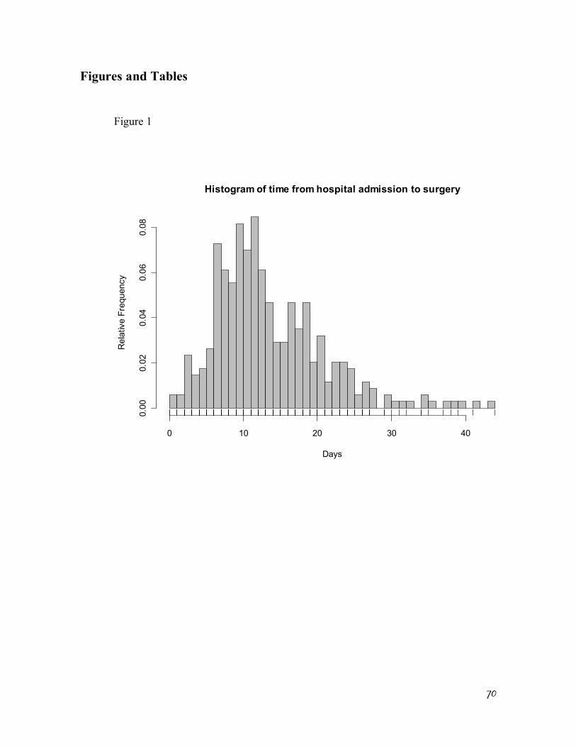
70
Figures and Tables
Figure 1
Histogram of time from hospital admission to surgery
Days
Rel
ativ
e Fr
eque
ncy
0 10 20 30 40
0.00
0.02
0.04
0.06
0.08
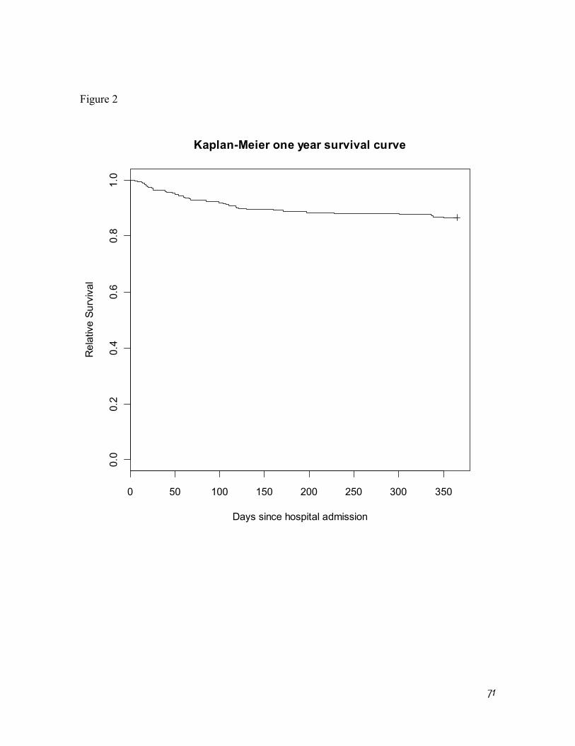
71
Figure 2
0 50 100 150 200 250 300 350
0.0
0.2
0.4
0.6
0.8
1.0
Kaplan-Meier one year survival curve
Days since hospital admission
Rel
ativ
e Su
rviv
al
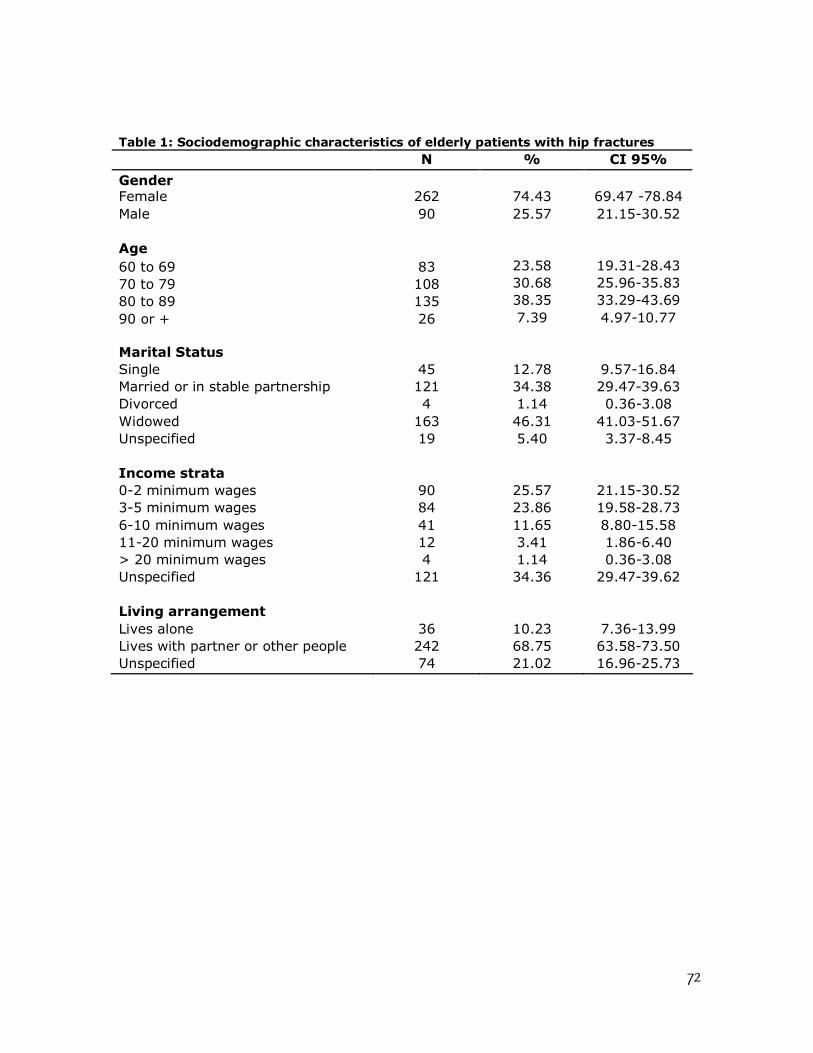
72
Table 1: Sociodemographic characteristics of elderly patients with hip fractures N % CI 95%
Gender Female 262 74.43 69.47 -78.84 Male 90 25.57 21.15-30.52 Age 60 to 69 83 23.58 19.31-28.43 70 to 79 108 30.68 25.96-35.83 80 to 89 135 38.35 33.29-43.69 90 or + 26 7.39 4.97-10.77 Marital Status Single 45 12.78 9.57-16.84 Married or in stable partnership 121 34.38 29.47-39.63 Divorced 4 1.14 0.36-3.08 Widowed 163 46.31 41.03-51.67 Unspecified 19 5.40 3.37-8.45 Income strata 0-2 minimum wages 90 25.57 21.15-30.52 3-5 minimum wages 84 23.86 19.58-28.73 6-10 minimum wages 41 11.65 8.80-15.58 11-20 minimum wages 12 3.41 1.86-6.40 > 20 minimum wages 4 1.14 0.36-3.08 Unspecified 121 34.36 29.47-39.62 Living arrangement Lives alone 36 10.23 7.36-13.99 Lives with partner or other people 242 68.75 63.58-73.50 Unspecified 74 21.02 16.96-25.73
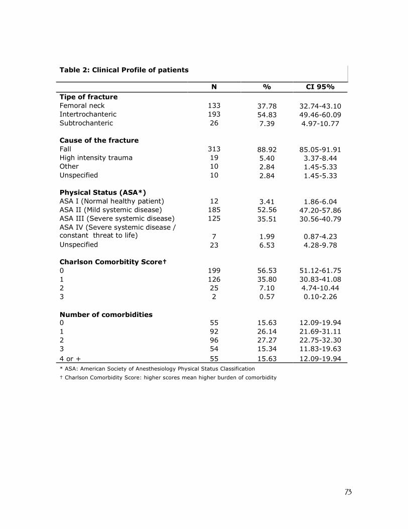
73
Table 2: Clinical Profile of patients
N % CI 95% Tipe of fracture Femoral neck 133 37.78 32.74-43.10 Intertrochanteric 193 54.83 49.46-60.09 Subtrochanteric 26 7.39 4.97-10.77 Cause of the fracture Fall 313 88.92 85.05-91.91 High intensity trauma 19 5.40 3.37-8.44 Other 10 2.84 1.45-5.33 Unspecified 10 2.84 1.45-5.33 Physical Status (ASA*) ASA I (Normal healthy patient) 12 3.41 1.86-6.04 ASA II (Mild systemic disease) 185 52.56 47.20-57.86 ASA III (Severe systemic disease) 125 35.51 30.56-40.79 ASA IV (Severe systemic disease / constant threat to life) 7 1.99 0.87-4.23 Unspecified 23 6.53 4.28-9.78 Charlson Comorbitity Score† 0 199 56.53 51.12-61.75 1 126 35.80 30.83-41.08 2 25 7.10 4.74-10.44 3 2 0.57 0.10-2.26 Number of comorbidities 0 55 15.63 12.09-19.94 1 92 26.14 21.69-31.11 2 96 27.27 22.75-32.30 3 54 15.34 11.83-19.63 4 or + 55 15.63 12.09-19.94 * ASA: American Society of Anesthesiology Physical Status Classification † Charlson Comorbidity Score: higher scores mean higher burden of comorbidity
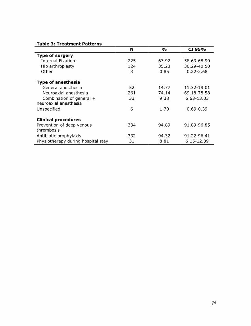
74
Table 3: Treatment Patterns N % CI 95%
Type of surgery Internal Fixation 225 63.92 58.63-68.90 Hip arthroplasty 124 35.23 30.29-40.50 Other 3 0.85 0.22-2.68 Type of anesthesia General anesthesia 52 14.77 11.32-19.01 Neuroaxial anesthesia 261 74.14 69.18-78.58 Combination of general + neuroaxial anesthesia
33 9.38 6.63-13.03
Unspecified 6 1.70 0.69-0.39 Clinical procedures Prevention of deep venous thrombosis
334 94.89 91.89-96.85
Antibiotic prophylaxis 332 94.32 91.22-96.41 Physiotherapy during hospital stay 31 8.81 6.15-12.39
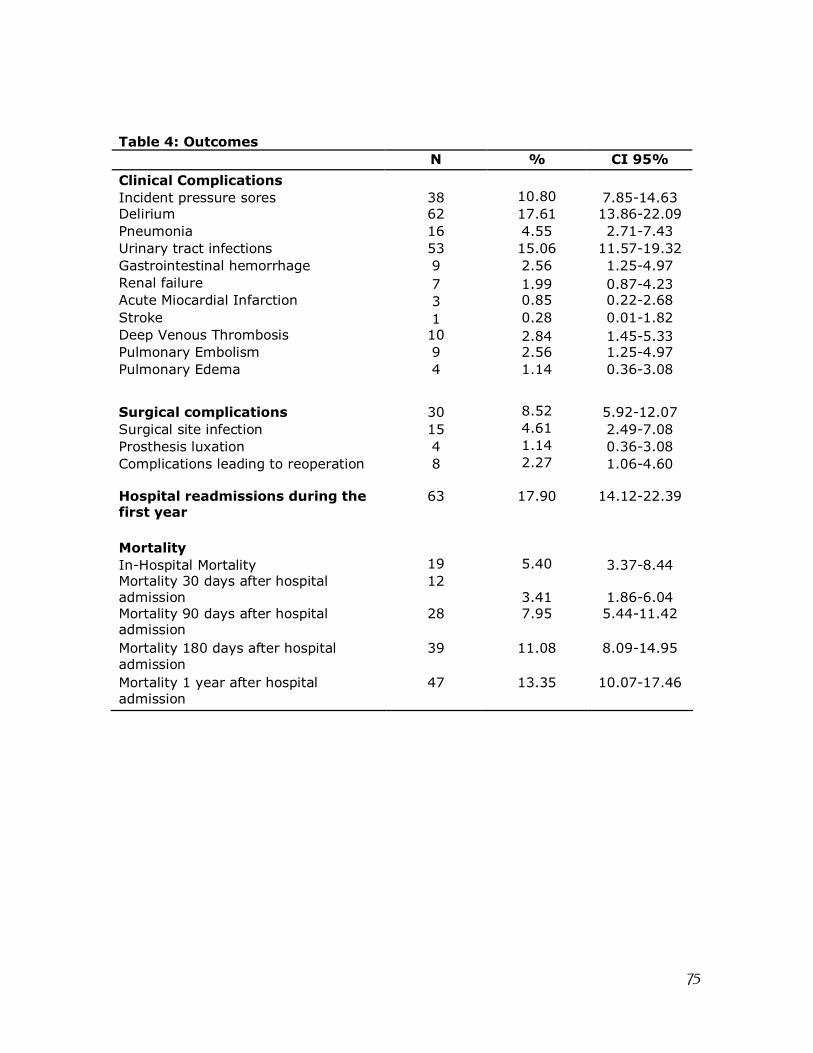
75
Table 4: Outcomes N % CI 95%
Clinical Complications Incident pressure sores 38 10.80 7.85-14.63 Delirium 62 17.61 13.86-22.09 Pneumonia 16 4.55 2.71-7.43 Urinary tract infections 53 15.06 11.57-19.32 Gastrointestinal hemorrhage 9 2.56 1.25-4.97 Renal failure 7 1.99 0.87-4.23 Acute Miocardial Infarction 3 0.85 0.22-2.68 Stroke 1 0.28 0.01-1.82 Deep Venous Thrombosis 10 2.84 1.45-5.33 Pulmonary Embolism 9 2.56 1.25-4.97 Pulmonary Edema 4 1.14 0.36-3.08 Surgical complications 30 8.52 5.92-12.07 Surgical site infection 15 4.61 2.49-7.08 Prosthesis luxation 4 1.14 0.36-3.08 Complications leading to reoperation 8 2.27 1.06-4.60 Hospital readmissions during the first year
63 17.90 14.12-22.39
Mortality In-Hospital Mortality 19 5.40 3.37-8.44 Mortality 30 days after hospital admission
12 3.41 1.86-6.04
Mortality 90 days after hospital admission
28 7.95 5.44-11.42
Mortality 180 days after hospital admission
39 11.08 8.09-14.95
Mortality 1 year after hospital admission
47 13.35 10.07-17.46
76
Acknowledgments: These authors (DCMF, CMC, RCS, RSP and KRCJr) were partially supported by research grants from the Brazilian National Council for Scientific and Technological Development (CNPq).
References
1. Cummings SR, Melton LJ. Epidemiology and outcomes of osteoporotic fractures.
Lancet. 2002 May 18;359(9319):1761-7.
2. Johnell O, Kanis J. An estimate of the worldwide prevalence, mortality and
disability associated with hip fracture. Osteoporos Int. 2004;15:897-902.
3. Johnell O. The socioeconomic burden of fractures: today and in the 21st century.
Am J Med. 1997 Aug 18;103(2A):20S-5S; discussion 5S-6S.
4. Gullberg B, Johnell O, Kanis JA. World-wide projections for hip fracture.
Osteoporos Int. 1997;7(5):407-13.
5. Castro da Rocha FA, Ribeiro AR. Low incidence of hip fractures in an equatorial
area. Osteoporos Int. 2003 Jul;14(6):496-9.
6. Vidal EI, Coeli CM, Pinheiro RS, Camargo KR, Jr. Mortality within 1 year after hip
fracture surgical repair in the elderly according to postoperative period: a probabilistic
record linkage study in Brazil. Osteoporos Int. 2006 Jul 27;17(10):1569-76.
7. Pinheiro MM, Ciconelli RM, Martini LA, Ferraz MB. Clinical risk factors for
osteoporotic fractures in Brazilian women and men: the Brazilian Osteoporosis Study
(BRAZOS). Osteoporos Int. 2008 Jul 3.
8. Komatsu RS, Ramos LR, Szejnfeld VL. Incidence of proximal femur fractures in
Marilia, Brazil. J Nutr Health Aging. 2004;8(5):362-7.
77
9. Morales-Torres J, Gutierrez-Urena S. The burden of osteoporosis in Latin America.
Osteoporos Int. 2004 Aug;15(8):625-32.
10. West of Scotland Coronary Prevention Study Group. Computerised record linkage:
compared with traditional patient follow-up methods in clinical trials and illustrated in a
prospective epidemiological study. J Clin Epidemiol. 1995 Dec;48(12):1441-52.
11. Jaro M. Probabilistic linkage of large public health data files. Stat Med. 1995 mar-
apr;14(5-7):491-8.
12. Machado J, Silveira D, Santos I, Piovesan M, Albuquerque C. [ The use of a
probabilistic record linkage methodology in databases to identify death records in
epidemiological studies]. Rev Bras Epidemiol. 2008;11(1):43-54.
13. Coeli C, Camargo Jr. K. [Evaluation of different blocking strategies in probabilistic
record linkage]. Rev Bras Epidemiol. 2002;5(2):185-96.
14. Shannon HS, Jamieson E, Walsh C, Julian JA, Fair ME, Buffet A. Comparison of
individual follow-up and computerized record linkage using the Canadian Mortality Data
Base. Can J Public Health. 1989 Jan-Feb;80(1):54-7.
15. Coutinho ES, Coeli CM. [Accuracy of the probabilistic record linkage methodology
to ascertain deaths in survival studies]. Cad Saude Publica. 2006 Oct;22(10):2249-52.
16. Camargo Jr. KR, Coeli CM. [Reclink: an application for database linkage
implementing the probabilistic record linkage method]. Cad Saude Publica. 2000 Apr-
Jun;16(2):439-47.
17. Charlson ME, Pompei P, Ales KL, MacKenzie CR. A new method of classifying
prognostic comorbidity in longitudinal studies: development and validation. J Chronic Dis.
1987;40(5):373-83.
78
18. R Development Core Team. R: A Language and Environment for Statistical
Computing. 2.7.1 ed. Vienna, Austria: R Foundation for Statistical Computing; 2008.
19. Vidal EI, Moreira-Filho DC, Coeli CM, Camargo KR, Jr., Fukushima FB, Blais R.
Hip fracture in the elderly: does counting time from fracture to surgery or from hospital
admission to surgery matter when studying in-hospital mortality? Osteoporos Int. 2009
May;20(5):723-9.
20. Ho V, Hamilton BH, Roos LL. Multiple approaches to assessing the effects of
delays for hip fracture patients in the United States and Canada. Health Serv Res.
2000;34(7):1499-518.
21. Orosz GM, Magaziner J, Hannan EL, Morrison RS, Koval K, Gilbert M, et al.
Association of timing of surgery for hip fracture and patient outcomes. Jama. 2004 Apr
14;291(14):1738-43.
22. Weller I, Wai EK, Jaglal S, Kreder HJ. The effect of hospital type and surgical
delay on mortality after surgery for hip fracture. J Bone Joint Surg Br. 2005 Mar;87(3):361-
6.
23. Shiga T, Wajima Z, Ohe Y. Is operative delay associated with increased mortality of
hip fracture patients? Systematic review, meta-analysis, and meta-regression. Can J
Anaesth. 2008 Mar;55(3):146-54.
24. National Services Scotland. Scottish Hip Fracture Audit report 2008. In: Division
IS, editor. Edinburgh: ISD Scotland Publications; 2008. p. 17.
25. Scottish Intercollegiate Guidelines Network. Prevention and management of hip
fracture in older people : a national clinical guideline. Edinburgh: SIGN; 2009.
79
26. Beaupre LA, Jones CA, Saunders LD, Johnston DW, Buckingham J, Majumdar SR.
Best practices for elderly hip fracture patients. A systematic overview of the evidence. J
Gen Intern Med. 2005 Nov;20(11):1019-25.
27. Lieberman JR, Romano PS, Mahendra G, Keyzer J, Chilcott M. The treatment of
hip fractures: variations in care. Clin Orthop Relat Res. 2006 Jan;442:239-44.
28. O'Hara DA, Duff A, Berlin JA, Poses RM, Lawrence VA, Huber EC, et al. The
effect of anesthetic technique on postoperative outcomes in hip fracture repair.
Anesthesiology. 2000 Apr;92(4):947-57.
29. Dickson RE, Patey RE. Anaesthesia for hip fracture: a survey of Scottish practice.
Scott Med J. 1999 Oct;44(5):152-4.
30. Parker MJ, Handoll HH, Griffiths R. Anaesthesia for hip fracture surgery in adults.
Cochrane Database Syst Rev. 2009(3):CD000521.
31. Magaziner J, Fredman L, Hawkes W, Hebel JR, Zimmerman S, Orwig DL, et al.
Changes in functional status attributable to hip fracture: a comparison of hip fracture
patients to community-dwelling aged. Am J Epidemiol. 2003 Jun 1;157(11):1023-31.
32. Nymark T, Lauritsen JM, Ovesen O, Röck ND, Jeune B. Decreasing incidence of
hip fracture in the Funen County, Denmark. Acta Orthop. 2006;77(1):109-13.
33. Finucane TE. How is geriatrics different from general internal medicine? Geriatrics
and Gerontology International. 2004;4(4):259-61.
81
Capítulo 3: The timing of surgery factor for older adults with hip fractures in a developing country
Edison Iglesias de Oliveira Vidal 1,2,3; Djalma de Carvalho Moreira-Filho2; Rejane
Sobrinho Pinheiro4; Rômulo Cristóvão de Souza5; Liz Maria de Almeida6; Kenneth Rochel
Camargo Jr7; Claudia Medina Coeli4
Affiliations:
1- State University of São Paulo – UNESP 2- Sate University of Campinas – UNICAMP 3- Albert Einstein Hospital – Sao Paulo 4- Federal University of Rio de Janeiro – UFRJ 5- Serra dos Órgãos Foundation 6- National Cancer Institute – INCA 7- State University of Rio de Janeiro - UERJ
Corresponding author:
Edison Iglesias de Oliveira Vidal
R. Pensilvânia 57, apto 233 B,
04564-000, São Paulo, SP, Brazil.
e-mail: [email protected]
Telephone: +55-11-34593007;
Fax: +55-11-37470715
82
Abstract Background: The association between delays to the surgical repair of Hip Fracture (HF)
and mortality persists as one of the most controversial issues in the study of the
epidemiology of those fractures. However, it remains largely unknown how this
relationship behaves in the context of developing countries, where a greater proportion of
patients are operated upon much later than 48h after hospital admission.
Methods: All medical records of patients aged 60 and older admitted to a University
Hospital in the city of Rio de Janeiro with a main diagnosis of HF between 1995 and 2000
were reviewed. The association between surgical timing, in-hospital complications and
patient survival was assessed by means of Logistic Regression and Cox Proportional
Hazards modeling.
Results: Among 343 patients there were 18 (5.3%) in-hospital deaths and 297 (86.6%)
patients were alive one year after surgery. The mean gaps from HF to hospital admission
and from hospital admission to surgery were 3.1 and 13 days, respectively. Even after
adjustment for the presence of other covariates the gap from fracture to hospital admission
remained a significant predictor of reduced survival to hospital discharge (HR: 1.13,
95%CI: 1.04 - 1.22, P = 0.004) and one year after admission (HR: 1.08, 95%CI: 1.04 -
1.12, P < 0.001).
Conclusion: Large delays from fracture to hospital admission might be associated with
reduced survival in the context of a developing country. Further studies should address in
more depth both the determinants and the consequences of large gaps from fracture to
hospital admission.
Keywords: Hip fracture; time to surgery, developing countries, mortality, epidemiology
83
Introduction
Hip Fractures (HF) represent the most severe of all the osteoporotic fractures and
remain an important cause of mortality, morbidity, dependency and costs for older adults
and healthcare systems worldwide 1-4. The association between delays to the surgical repair
of HF and mortality, as well as what should be considered “the optimal timing” for this
surgical procedure persist as some of the most controversial issues in the medical literature
devoted to the study of the epidemiology of those fractures in elderly populations 5-12. As a
matter of fact, the two most recent systematic reviews examining this issue arrived at
opposite conclusions regarding the association of early or later surgical timing and patient
survival 13, 14.
Noticeably, most studies regarding this subject were conducted in developed
countries, where the majority of elderly patients with a HF are operated upon in less than
48h from hospital admission and the main study question was usually directed toward the
assessment of any significant difference in mortality between patients undergoing HF repair
early (i.e. in the first 12 or 24h after hospital admission) or later on. However, it remains
largely unknown how this relationship between surgical timing and mortality behaves in
the context of developing countries, where a greater proportion of patients are operated
upon much later than 48h from hospital admission. Understanding this and other aspects of
the epidemiology of HF in developing countries is highly relevant since it is precisely in
those countries where the greatest rise in the incidence and burden of HF is expected in the
near future 15. Hence, we conducted an observational retrospective study analyzing the
association between the timing of surgical HF repair and patient mortality in one University
84
Hospital responsible for a substantial share of all HF surgeries in the city of Rio de Janeiro,
in the Southeast of Brazil.
Methods All medical records of patients aged 60 and older with a main admission diagnosis
of HF between 1995 and 2000 were retrospectively reviewed and abstracted according to a
standardized instrument previously tested. Patients whose HF was related to a malignancy,
who did not undergo surgical repair or whose date of fracture was unknown were excluded.
In order to assess the one year survival and mortality rates of the study patients,
records were linked to the database of the Brazilian Mortality Information System from
1995 to 2001 by means of Probabilistic Record Linkage Methodology (PRLM) 16-21.
Previous research in a similar setting revealed 85.5% sensitivity, 99.4% specificity, 98.1%
and 94.9% positive and negative predictive values, respectively, regarding correct matching
of records between databases according to this methodological approach 22. The RecLink II
Software 23 was used for the implementation of PRLM followed by manual examination of
pairs of records with higher probability of representing a true match between databases.
The association between patient survival to hospital discharge and at one year after
fracture and the timing of surgery was assessed by means of univariate and multiple Cox
Proportional Hazards modeling 24. The time to surgery factor was analyzed both in terms of
total time from fracture to surgery and in terms of its subcomponents (i.e. time from
fracture to hospital admission and time from admission to surgery). The univariate
associations between the surgical timing and survival were further adjusted according to the
following variables: type of HF, type of surgical treatment and anesthetic technique,
85
comorbidity burden as measured by the Charlson Index 25, American Society of
Anesthesiology (ASA) physical status score as ascertained prior to surgery, use of
antithrombotic and antibiotic prophylaxis and occurrence of in-hospital physiotherapy care.
For illustrative Kaplan-Meier one year survival curve was plotted stratifying patients into
those who were admitted to the hospital with three days or less after the fracture and those
who were admitted later on. A log-rank test was performed examining the crude difference
between these two strata.
Further assessments regarding the association between surgical timing and the
incidence of grade II or higher pressure ulcers, pulmonary embolism, mental confusion,
pneumonia and a composite of multiple clinical complications were performed by means of
logistic regression modeling following the adjustment by the same variables listed
previously. The composite measure of clinical complications encompassed the occurrence
of any of the following diagnoses during hospital stay: myocardial infarction, renal failure,
pulmonary edema, bowel obstruction, pneumonia, urinary tract infection, grade II or higher
pressure ulcer, deep vein thrombosis, pulmonary embolism and gastrointestinal bleeding.
Each diagnosis was retrospectively ascertained according to available medical records. In a
similar way the relationship between time to surgery and the length of hospital stay was
analyzed by means of Cox proportional hazards modeling after subtraction of the total
length of stay by the number of days awaiting surgery (i.e. time to hospital discharge after
surgery).
All statistical analyses were performed using the R software version 2.10.1 26. The
level of α for statistical significance was set at 0.05.
86
Results
Among the 343 patients fulfilling the study’s inclusion criteria, there were 256
(74.6%) women. The mean age overall was 77.4 years. The mean length of stay was 20.5
days with an interquartile range of 14 to 24 days. The mean time from the occurrence of the
HF to hospital admission was 3.1 days (interquartile range: 0-4 days) and the mean gap
from hospital admission to surgery was 13 days (interquartile range: 8-17 days). There were
18 (5.3%) in-hospital deaths and 297 (86.6%) of all patients were alive one year after
surgery. A total of 36 (10.5%) and eight (2.3%) patients developed a pressure ulcer or
pulmonary embolism during the index hospitalization period, respectively.
Table 1 depicts the results of Cox proportional hazards regression examining the
association between the timing of surgery and in-hospital and one year survival as well as
the length of hospital stay after surgery, both before and after adjustment for the presence
of other covariates previously cited. The analysis of Schoenfeld residuals revealed that the
underlying proportional hazards assumption of Cox regression modeling was respected.
Figure 1 portrays the one year Kaplan-Meier survival curve stratified according to the gap
from fracture to hospital admission. The log-rank test revealed a statistically significant
difference regarding the one-year survival of patients admitted before three days from the
occurrence of the HF or thereafter (P: 0.00015). Table 2 displays the results of logistic
regression analyzing the association between surgical timing and the occurrence of in-
hospital pressure ulcers, pulmonary embolism and mental confusion. Table 3 describes the
different baseline clinical profiles of patients according to the timing of hospitalization.
87
Discussion
For a long time the subject of optimal early timing for HF surgical repair was
considered a dogma among orthopedic surgeons 27, until it was first questioned in 1984 by
Kenzora et al, who described greater mortality rates for HF patients operated upon less than
24h after hospital admission 27. Thereafter, this subject has been reexamined and reviewed
many times in different contexts and by a variety of methodological approaches,
nevertheless this debate appears far from an end 28.
It is critical to consider certain limitations concerning the medical literature
analyzing the relationship between the gap from fracture to surgery and mortality. First,
most if not all studies have been conducted in developed countries, where the great
majority of patients undergoes surgery in the first 48h of hospital admission. It is likely that
in many other developing countries, as in the present case, most patients have access to the
surgical theatre much later on. Second, most studies did not consider in their analyses the
total gap from fracture to surgery, but only the time interval between hospital admission
and surgery. Therefore, those studies implicitly assumed these two gaps to be equivalent 28.
It is noteworthy that in the current context of a developing country, this assumption does
not apply. This remark must be taken into account in the design of future studies on the
epidemiology of HF in developing countries.
Quite interesting is the current finding of an association between the gap from
fracture to hospital admission and both in-hospital and one year mortality, even after
adjustment for other potential confounders (table 1). According to those findings, each day
of delay from fracture to hospital admission is associated with a 4% to 12% increased risk
of death at one year and 4% to 22% greater risk of dying during the current episode of
88
hospital admission. Indeed, it appears that the association between the total gap from
fracture to surgery and one year mortality is entirely accountable to this pre-hospital
admission delay. On the other hand, the gap from hospital admission to HF surgical repair
was not found to be a significant predictor of in-hospital and of one year mortality (after
adjustment). Moreover, at least for the in-hospital survival analysis, a non-significant trend
was observed in the opposite direction, suggesting that delayed surgery could be associated
with a little lower in-hospital mortality, possibly because sicker patients, who needed
clinical stabilization for acute medical problems, did benefit from later surgery, after
appropriate medical management.
These different patterns of association between the two subcomponents of the total
gap from fracture to surgery and mortality should not be considered a paradoxical finding.
In fact, they may reflect different underlying mechanisms. For instance, large delays from
fracture to hospital admission might primarily mirror problems either in the access to health
care or in the recognition of the severity of a HF by the patient and / or his / hers caregivers
(i.e. more dependent and frail patients, with worse patterns of care). Whereas delays from
hospital admission to surgery might suggest a wider array of factors, ranging from the need
for clinical stabilization of acute medical problems, to logistical difficulties and local
priorities in the allocation of surgical theatre time.
According to the present study the mechanism underlying the association between
the timing of hospital admission and mortality cannot be attributed to the occurrence of
pressure ulcers, pulmonary embolism, mental confusion, pneumonia, nor a composite of
clinical complications (table 2). Furthermore, the comparison of a minimum set of
demographic and clinical characteristics, HF patients being admitted to the hospital with
different timings after fracture do not appear significantly different from each other (table
89
3). However, the hypothesis that other unmeasured variables do play a role as confounders
for this association can not be excluded on the basis of the present data, which, therefore,
must be interpreted with caution. Notwithstanding, even if this were the case, it could be
argued with more confidence that large gaps from fracture to hospital admission could still
serve as markers of patients at higher risk for mortality.
This study encompasses several limitations, which must me considered. First, the
study design is observational, which makes it more prone to bias than clinical trials 29.
However, observational studies are the only alternative for issues such as the one examined
here, where ethical and logistical reasons make randomized clinical trials unfeasible 5, 11, 12
– i.e. it would be considered unethical to randomly allocate patients to later surgery, since
unnecessary waiting is likely to be associated with pain, immobility and suffering for
patients. Second, it was not possible to control properly for other important variables, such
as nutritional, socioeconomic and mental status prior to the fracture, severity of the HF,
pain control, and health care patterns after hospital discharge, among other variables.
Hence, as previously appointed, the current results must be interpreted with parsimony and
foster further investigations regarding both the determinants and the consequences of the
gaps from fracture to hospital admission. Third, we were not able to consider the different
reasons for the delays to hospital admission (e.g. patients might have been first admitted to
another hospital without orthopedic surgical facilities and therefore were transferred later to
the University hospital, where the HF repair took place). Yet, this concern by itself does not
refute the association between reduced survival and the gap to admission to the hospital
where the HF is in fact repaired. Rather, it highlights the matter of proper access to health
care as an underlying factor associated with reduced survival for elderly patients. Fourth,
the present results are not generalizable to the whole city of Rio de Janeiro nor to other
90
regions of the country. Nevertheless, it is not unreasonable to consider that the current
findings should hold a certain relationship to the patterns of care from other hospitals in the
same region and even in other major cities of the country, due to the function of University
Hospitals in the education of healthcare professionals and even as role models in the
healthcare system.
Conclusion
The gap from fracture to hospital admission, which has generally deserved less
attention from most studies on the epidemiology of HF in developed countries, might be a
relevant marker of short- and long-term mortality in developing countries. Further
understanding of the determinants and consequences of late surgical timing for HF patients
appears important for the design of elder friendly Public Health Policies in the context of an
aging World.
Acknowledgments:
These authors (DCMF, CMC, RCS, RSP and KRCJr) were partially supported by
research grants from the Brazilian National Council for Scientific and Technological
Development (CNPq).
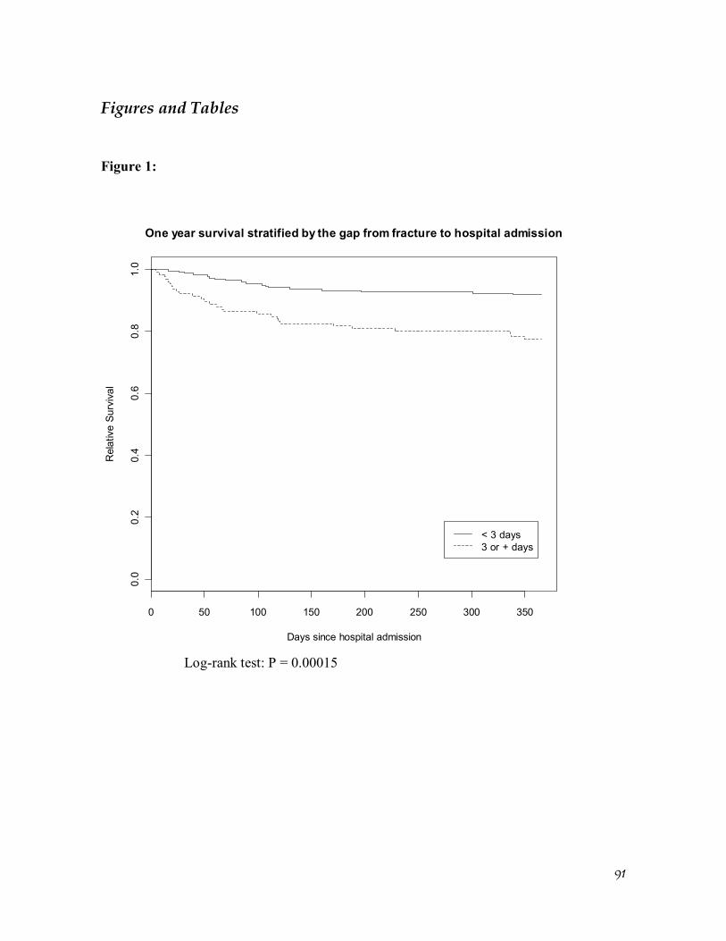
91
Figures and Tables Figure 1:
0 50 100 150 200 250 300 350
0.0
0.2
0.4
0.6
0.8
1.0
One year survival stratified by the gap from fracture to hospital admission
Days since hospital admission
Rel
ativ
e Su
rviv
al
< 3 days3 or + days
Log-rank test: P = 0.00015
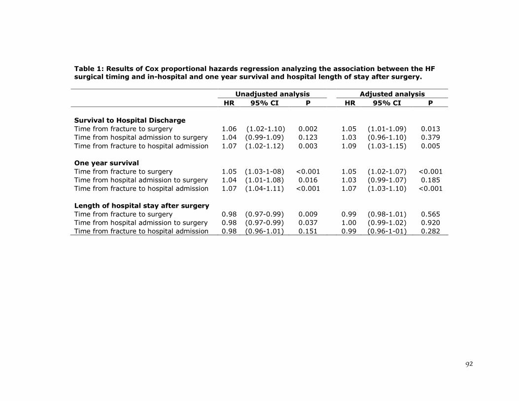
92
Table 1: Results of Cox proportional hazards regression analyzing the association between the HF surgical timing and in-hospital and one year survival and hospital length of stay after surgery. Unadjusted analysis Adjusted analysis HR 95% CI P HR 95% CI P Survival to Hospital Discharge Time from fracture to surgery 1.06 (1.02-1.10) 0.002 1.05 (1.01-1.09) 0.013 Time from hospital admission to surgery 1.04 (0.99-1.09) 0.123 1.03 (0.96-1.10) 0.379 Time from fracture to hospital admission 1.07 (1.02-1.12) 0.003 1.09 (1.03-1.15) 0.005 One year survival Time from fracture to surgery 1.05 (1.03-1-08) <0.001 1.05 (1.02-1.07) <0.001 Time from hospital admission to surgery 1.04 (1.01-1.08) 0.016 1.03 (0.99-1.07) 0.185 Time from fracture to hospital admission 1.07 (1.04-1.11) <0.001 1.07 (1.03-1.10) <0.001 Length of hospital stay after surgery Time from fracture to surgery 0.98 (0.97-0.99) 0.009 0.99 (0.98-1.01) 0.565 Time from hospital admission to surgery 0.98 (0.97-0.99) 0.037 1.00 (0.99-1.02) 0.920 Time from fracture to hospital admission 0.98 (0.96-1.01) 0.151 0.99 (0.96-1-01) 0.282
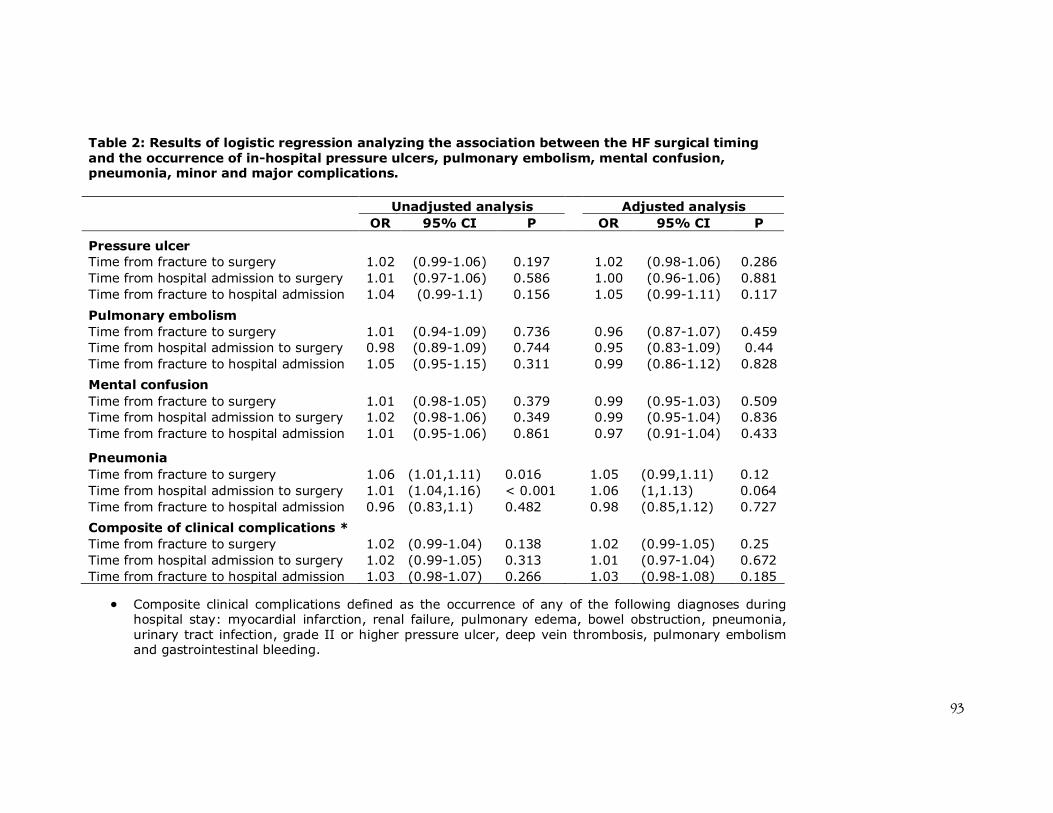
93
Composite clinical complications defined as the occurrence of any of the following diagnoses during hospital stay: myocardial infarction, renal failure, pulmonary edema, bowel obstruction, pneumonia, urinary tract infection, grade II or higher pressure ulcer, deep vein thrombosis, pulmonary embolism and gastrointestinal bleeding.
Table 2: Results of logistic regression analyzing the association between the HF surgical timing and the occurrence of in-hospital pressure ulcers, pulmonary embolism, mental confusion, pneumonia, minor and major complications.
Unadjusted analysis Adjusted analysis OR 95% CI P OR 95% CI P
Pressure ulcer Time from fracture to surgery 1.02 (0.99-1.06) 0.197 1.02 (0.98-1.06) 0.286 Time from hospital admission to surgery 1.01 (0.97-1.06) 0.586 1.00 (0.96-1.06) 0.881 Time from fracture to hospital admission 1.04 (0.99-1.1) 0.156 1.05 (0.99-1.11) 0.117
Pulmonary embolism Time from fracture to surgery 1.01 (0.94-1.09) 0.736 0.96 (0.87-1.07) 0.459 Time from hospital admission to surgery 0.98 (0.89-1.09) 0.744 0.95 (0.83-1.09) 0.44 Time from fracture to hospital admission 1.05 (0.95-1.15) 0.311 0.99 (0.86-1.12) 0.828
Mental confusion Time from fracture to surgery 1.01 (0.98-1.05) 0.379 0.99 (0.95-1.03) 0.509 Time from hospital admission to surgery 1.02 (0.98-1.06) 0.349 0.99 (0.95-1.04) 0.836 Time from fracture to hospital admission 1.01 (0.95-1.06) 0.861 0.97 (0.91-1.04) 0.433
Pneumonia Time from fracture to surgery 1.06 (1.01,1.11) 0.016 1.05 (0.99,1.11) 0.12 Time from hospital admission to surgery 1.01 (1.04,1.16) < 0.001 1.06 (1,1.13) 0.064 Time from fracture to hospital admission 0.96 (0.83,1.1) 0.482 0.98 (0.85,1.12) 0.727
Composite of clinical complications * Time from fracture to surgery 1.02 (0.99-1.04) 0.138 1.02 (0.99-1.05) 0.25 Time from hospital admission to surgery 1.02 (0.99-1.05) 0.313 1.01 (0.97-1.04) 0.672 Time from fracture to hospital admission 1.03 (0.98-1.07) 0.266 1.03 (0.98-1.08) 0.185
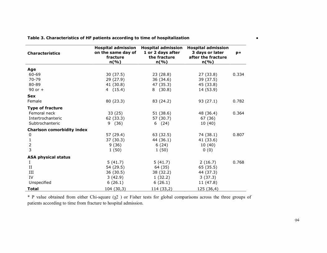
94
* P value obtained from either Chi-square (χ2 ) or Fisher tests for global comparisons across the three groups of patients according to time from fracture to hospital admission.
Table 3. Characteristics of HF patients according to time of hospitalization
Characteristics P*
Hospital admission on the same day of
fracture n(%)
Hospital admission 1 or 2 days after
the fracture n(%)
Hospital admission 3 days or later
after the fracture n(%)
Age 60-69 30 (37.5) 23 (28.8) 27 (33.8) 0.334 70-79 29 (27.9) 36 (34.6) 39 (37.5) 80-89 41 (30.8) 47 (35.3) 45 (33.8) 90 or + 4 (15.4) 8 (30.8) 14 (53.9)
Sex Female 80 (23.3) 83 (24.2) 93 (27.1) 0.782
Type of fracture Femoral neck 33 (25) 51 (38.6) 48 (36.4) 0.364 Intertrochanteric 62 (33.3) 57 (30.7) 67 (36) Subtrochanteric 9 (36) 6 (24) 10 (40)
Charlson comorbidity index 0 57 (29.4) 63 (32.5) 74 (38.1) 0.807 1 37 (30.3) 44 (36.1) 41 (33.6) 2 9 (36) 6 (24) 10 (40) 3 1 (50) 1 (50) 0 (0)
ASA physical status I 5 (41.7) 5 (41.7) 2 (16.7) 0.768 II 54 (29.5) 64 (35) 65 (35.5) III 36 (30.5) 38 (32.2) 44 (37.3) IV 3 (42.9) 1 (32.2) 3 (37.3) Unspecified 6 (26.1) 6 (26.1) 11 (47.8)
Total 104 (30,3) 114 (33,2) 125 (36,4)
95
References 1. Cummings SR, Melton LJ. Epidemiology and outcomes of osteoporotic
fractures. Lancet. 2002 May 18;359(9319):1761-7.
2. Johnell O, Kanis J. An estimate of the worldwide prevalence, mortality and
disability associated with hip fracture. Osteoporos Int. 2004;15:897-902.
3. Johnell O, Kanis JA. Epidemiology of osteoporotic fractures. Osteoporos Int.
2005 Mar;16 Suppl 2:S3-7.
4. Johnell O. The socioeconomic burden of fractures: today and in the 21st century.
Am J Med. 1997 Aug 18;103(2A):20S-5S; discussion 5S-6S.
5. McGuire K, Bernstein J, Polsky D, Silber J. Delays until surgery after hip
fracture increases mortality. Clin Orthop Rel Res. 2004 November;428:294-301.
6. Grimes JP, Gregory PM, Noveck H, Butler MS, Carson JL. The effects of time-
to-surgery on mortality and morbidity in patients following hip fracture. Am J Med.
2002 Jun 15;112(9):702-9.
7. Majumdar SR, Beaupre LA, Johnston DW, Dick DA, Cinats JG, Jiang HX. Lack
of association between mortality and timing of surgical fixation in elderly patients with
hip fracture: results of a retrospective population-based cohort study. Med Care. 2006
Jun;44(6):552-9.
8. Rae HC, Harris IA, McEvoy L, Todorova T. Delay to surgery and mortality after
hip fracture. ANZ J Surg. 2007 Oct;77(10):889-91.
9. Novack V, Jotkowitz A, Etzion O, Porath A. Does delay in surgery after hip
fracture lead to worse outcomes? A multicenter survey. Int J Qual Health Care. 2007
Jun;19(3):170-6.
96
10. Orosz GM, Magaziner J, Hannan EL, Morrison RS, Koval K, Gilbert M, et al.
Association of timing of surgery for hip fracture and patient outcomes. Jama. 2004 Apr
14;291(14):1738-43.
11. Zuckerman JD, Skovron ML, Koval KJ, Aharonoff G, Frankel VH.
Postoperative complications and mortality associated with operative delay in older
patients who have a fracture of the hip. J Bone Joint Surg Am. 1995 Oct;77(10):1551-6.
12. Casaletto JA, Gatt R. Post-operative mortality related to waiting time for hip
fracture surgery. Injury. 2004 Feb;35(2):114-20.
13. Shiga T, Wajima Z, Ohe Y. Is operative delay associated with increased
mortality of hip fracture patients? Systematic review, meta-analysis, and meta-
regression. Can J Anaesth. 2008 Mar;55(3):146-54.
14. Khan SK, Kalra S, Khanna A, Thiruvengada MM, Parker MJ. Timing of surgery
for hip fractures: a systematic review of 52 published studies involving 291,413
patients. Injury. 2009;40(7):692-7.
15. Gullberg B, Johnell O, Kanis JA. World-wide projections for hip fracture.
Osteoporos Int. 1997;7(5):407-13.
16. West of Scotland Coronary Prevention Study Group. Computerised record
linkage: compared with traditional patient follow-up methods in clinical trials and
illustrated in a prospective epidemiological study. J Clin Epidemiol. 1995
Dec;48(12):1441-52.
17. Jaro M. Probabilistic linkage of large public health data files. Stat Med. 1995
mar-apr;14(5-7):491-8.
18. Vidal EI, Coeli CM, Pinheiro RS, Camargo KR, Jr. Mortality within 1 year after
hip fracture surgical repair in the elderly according to postoperative period: a

97
probabilistic record linkage study in Brazil. Osteoporos Int. 2006 Jul 27;17(10):1569-
76.
19. Machado J, Silveira D, Santos I, Piovesan M, Albuquerque C. [ The use of a
probabilistic record linkage methodology in databases to identify death records in
epidemiological studies]. Rev Bras Epidemiol. 2008;11(1):43-54.
20. Coeli C, Camargo Jr. K. [Evaluation of different blocking strategies in
probabilistic record linkage]. Rev Bras Epidemiol. 2002;5(2):185-96.
21. Shannon HS, Jamieson E, Walsh C, Julian JA, Fair ME, Buffet A. Comparison
of individual follow-up and computerized record linkage using the Canadian Mortality
Data Base. Can J Public Health. 1989 Jan-Feb;80(1):54-7.
22. Coutinho ES, Coeli CM. [Accuracy of the probabilistic record linkage
methodology to ascertain deaths in survival studies]. Cad Saude Publica. 2006
Oct;22(10):2249-52.
23. Camargo Jr. KR, Coeli CM. [Reclink: an application for database linkage
implementing the probabilistic record linkage method]. Cad Saude Publica. 2000 Apr-
Jun;16(2):439-47.
24. Carvalho MS, Andreozzi VL, Codeço CT, Barbosa MTS, Shimakura SE.
[Survival analysis: theory and practice in health care]. 1a ed. Rio de Janeiro: Fiocruz;
2005.
25. Charlson ME, Pompei P, Ales KL, MacKenzie CR. A new method of classifying
prognostic comorbidity in longitudinal studies: development and validation. J Chronic
Dis. 1987;40(5):373-83.
26. R Development Core Team. R: A Language and Environment for Statistical
Computing. 2.10.1 ed. Vienna, Austria: R Foundation for Statistical Computing; 2009.
98
27. Kenzora JE, McCarthy RE, Lowell JD, Sledge CB. Hip fracture mortality.
Relation to age, treatment, preoperative illness, time of surgery, and complications. Clin
Orthop Relat Res. 1984 Jun(186):45-56.
28. Vidal EI, Moreira-Filho DC, Coeli CM, Camargo KR, Jr., Fukushima FB, Blais
R. Hip fracture in the elderly: does counting time from fracture to surgery or from
hospital admission to surgery matter when studying in-hospital mortality? Osteoporos
Int. 2009 May;20(5):723-9.
29. Bhandari M, Tornetta P, 3rd, Ellis T, Audige L, Sprague S, Kuo JC, et al.
Hierarchy of evidence: differences in results between non-randomized studies and
randomized trials in patients with femoral neck fractures. Arch Orthop Trauma Surg.
2004 Jan;124(1):10-6.
99
Discussão Geral
A temática das FFP em idosos corresponde a um campo profícuo de
investigação epidemiológica em função de sua relevância e das múltiplas abordagens
possíveis ao assunto. Na presente pesquisa foram abordados certos aspectos desta
epidemiologia com o objetivo de tentar suprir algumas poucas das muitas lacunas que
permeiam a literatura desta área.
Dentro do contexto de uma base de dados canadenses investigou-se a questão da
utilização do intervalo de tempo entre a hospitalização e a cirurgia enquanto um
substituto para o intervalo de maior relevância biológica entre a fratura propriamente
dita e a cirurgia (52) enquanto preditor da ocorrência de óbito no período pós-
operatório. O exame da hipótese de intercambialidade destes dois intervalos de tempo
possibilitou por um lado criar evidência inicial acerca de uma suposição amplamente
adotada, mas não previamente testada, por muitos estudos anteriores. Por outro lado, o
processo de pesquisa envolvido na confecção daquele manuscrito também desvelou uma
outra lacuna que permeia o conhecimento sobre a epidemiologia das FFP e que seria
novamente ressaltada através dos dois estudos subseqüentes realizados na cidade do Rio
de Janeiro. Trata-se da questão da caracterização dos fatores associados a
hospitalizações tardias de pacientes idosos portadores de uma FQ.
A descrição do perfil clínico, dos padrões de tratamento hospitalar bem como
dos desfechos quanto a complicações intra-hospitalares e à sobrevivência em um ano de
idosos brasileiros atendidos em um hospital universitário da cidade do Rio de Janeiro
revelaram alguns dados interessantes não apenas a respeito das características dos
pacientes, mas também sobre o processo de atenção à saúde dos idosos. Dentre eles
destacam-se um perfil clínico com menor proporção de comprometimento funcional e
100
carga de co-morbidades em relação a estudos provenientes de países desenvolvidos; a
grande demora para a realização do procedimento cirúrgico reparador e mesmo para o
acesso à internação hospitalar, além da baixa freqüência de assistência fisioterápica
durante a internação.
A análise da relação entre o timing cirúrgico e a mortalidade dos idosos
acometidos por uma FQ além de levantar a possibilidade de uma associação
principalmente no que concerne à demora para o acesso à hospitalização e a menor
sobrevida, ratificou a necessidade de futuros estudos buscando compreender os
determinantes e as conseqüências da hospitalização tardia, em especial no contexto dos
países em desenvolvimento.
FFP enquanto evento sentinela para a atenção à saúde do idoso
O conceito de evento sentinela no campo da saúde remonta à década de 70 do
século passado, quando Rutstein et al (53), frente à dificuldade conceitual e operacional
para identificar e quantificar medidas objetivas de gradientes positivos de saúde (ex:
“boa saúde”, “saúde mediana” e “saúde ruim”), propõem uma alternativa para a
mensuração da qualidade da atenção à saúde. Esta alternativa metodológica consistia no
registro de índices negativos de saúde, através da contagem de doenças, incapacidades e
mortes evitáveis (53). Estes índices negativos por quantificar seriam os eventos
sentinelas em saúde, os quais por sua vez corresponderiam a “uma doença, incapacidade
ou morte precoce, cuja ocorrência serve como um sinal de alerta de que a qualidade de
cuidados preventivos e / ou terapêuticos pode requerer melhorias” (54, p. 1054)
(tradução livre). Seriam eventos para os quais dever-se-ia questionar os porquês de sua
ocorrência. Ainda nas palavras dos autores: “A identificação dos motivos para ‘quedas
de aviões na saúde’ é muito mais simples, mais direta e menos custosa em termos de
101
tempo, dinheiro e recursos humanos que a abordagem global de observação de
populações inteiras para a ocorrência de fatores que prejudiquem sua saúde” (53)
(p.583) (tradução livre).
Seguindo esta linha de raciocínio foram elaboradas àquela época, a partir do
auxílio de diversos especialistas, três listas de eventos sentinelas em saúde (53). A
primeira lista englobava aquelas condições para as quais havia além de consenso e
clareza acerca de sua evitabilidade, a possibilidade de aplicação imediata para a
mensuração da qualidade dos cuidados de saúde da população. Esta lista incluía
condições como difteria, cólera, sarampo, carências nutricionais, mortes maternas,
osteomielite, neoplasias associadas ao tabaco e patologias ocupacionais, dentre muitas
outras. A ocorrência de um único evento pertencente a esta lista seria suficiente para
justificar o questionamento sobre seus motivos subjacentes. A segunda lista
correspondia a condições para as quais a prevenção e / ou tratamento seriam altamente
efetivos, no entanto o evento de um único caso não seria suficiente para deflagrar
investigações sobre suas causas básicas. Estas seriam desencadeadas apenas frente a
mudanças significativas nas taxas usuais de ocorrência. Esta segunda listagem de
patologias incluía, por exemplo, câncer de cólon, infecções hospitalares, cáries,
hipertensão arterial e doenças vasculares a ela relacionadas. A terceira lista identificava
condições capazes de afetar intensamente a saúde, mas para as quais não havia àquele
momento estratégias suficientemente bem estabelecidas para sua prevenção, tratamento
e / ou diagnóstico a ponto de justificar sua inclusão enquanto indicadores da qualidade
da atenção à saúde. Estas condições incluíam as doenças mentais, problemas associados
ao alcoolismo e uso de drogas ilícitas, suicídios e homicídios.
Duas particularidades devem ser ressaltadas em relação à estas listas de eventos
sentinela elaboradas por Rutstein et al (53). A primeira envolve a explicitação pelos
102
autores de que a evolução do conhecimento científico e as mudanças nas condições
sociais, ambientais e de cuidado à saúde tornam compulsórias atualizações periódicas
das listas de eventos sentinela à luz dos novos tempos. A segunda particularidade refere-
se ao fato de os autores terem sistematicamente excluído eventos associados a pessoas
com 65 anos ou mais de idade (55). Este último elemento correlaciona-se
provavelmente com o perfil demográfico característico daquela época e com a noção
errônea e infelizmente ainda presente nos dias de hoje, de que os agravos à saúde dos
idosos são “naturais da idade”, e não um produto da interação dos efeitos da passagem
do tempo modulados intensamente por condições sociais, fatores genéticos, hábitos e
escolhas e vida (56, 57).
Não é difícil argumentar que, frente ao fenômeno do envelhecimento
populacional mundial e aos avanços sobre a própria compreensão do envelhecer
humano, o século XXI demanda por atualizações para as listas de agravos evitáveis à
saúde incorporando definitivamente a população idosa. Apesar de já terem sido
propostas como eventos sentinela (55), as FFP não têm sido utilizadas com esta
finalidade para a avaliação e o monitoramento da qualidade da atenção à saúde dos
idosos (55, 58-61).
A incorporação das FFP de forma efetiva para o monitoramento da saúde dos
idosos revela uma série de vantagens potenciais para os sistemas de saúde, conforme
listadas a seguir.
Facilidade para identificação de casos utilizando sistemas de informação
hospitalar;
Diagnóstico preciso envolvendo tecnologias simples;
103
Desfechos significativos aferíveis em curto prazo através de sistemas de
informação também amplamente disponíveis (ex: óbito);
Refletir aspectos da atenção à saúde do idoso desde a prevenção primária
à prevenção terciária§.
Em função dos elementos citados acima, argumenta-se que as FFP devam ser
entendidas como um evento sentinela bastante interessante e adequado para o
monitoramento da qualidade da atenção à saúde dos idosos. Seguindo a esquematização
de categorias de eventos sentinela previamente citada, as FFP enquadrar-se-iam no
primeiro tipo de eventos, i.e. aqueles para os quais a ocorrência de um único caso seria
suficiente para que se questione: “por que isto aconteceu?” Desta forma, para cada idoso
que tenha sofrido uma FFP caberia levantar as raízes causais envolvidas tanto na gênese
da fratura em si, como dos desfechos de reabilitação e mortalidade subseqüentes.
Espera-se que a incorporação das FQ enquanto um indicador da qualidade da atenção à
saúde prestada aos idosos possa contribuir para o necessário processo de melhoria
destes cuidados bem como para o desenvolvimento de políticas públicas voltadas para
esta população.
§§ Prevenção primária enquanto prevenção de quedas e tratamento da osteoporose. Prevenção secundária: acesso a tratamento hospitalar adequado e profilaxia de complicações precoces. Prevenção terciária na forma de reabilitação e prevenção de novas fraturas e complicações tardias.
105
Conclusão geral
As FFP correspondem a um objeto de estudo privilegiado e extremamente
relevante para a Saúde Pública dentro da perspectiva de um mundo em envelhecimento.
A maior compreensão de sua epidemiologia é fundamental para o desenho de políticas
públicas favoráveis aos idosos. Trata-se de um vasto campo de pesquisa, cuja
abordagem se faz possível através de pequenos “recortes”, como os representados pelos
três estudos que compõem esta pesquisa. É importante notar que os três estudos
descritos apresentam importantes limitações, que, todavia, não os impede de contribuir
de forma singular e criativa para crescimento do conhecimento acerca deste tema. Por
fim, argumenta-se a favor das FFP enquanto um possível evento sentinela da saúde do
idoso tanto no âmbito nacional como internacional.
107
Referências
1. Johnell O. The socioeconomic burden of fractures: today and in the 21st century.
Am J Med. 1997 Aug 18;103(2A):20S-5S; discussion 5S-6S.
2. Johnell O, Kanis J. An estimate of the worldwide prevalence, mortality and
disability associated with hip fracture. Osteoporos Int. 2004;15:897-902.
3. Gullberg B, Johnell O, Kanis JA. World-wide projections for hip fracture.
Osteoporos Int. 1997;7(5):407-13.
4. Cooper C, Campion C, Melton III LJ. Hip fractures in the elderly: world wide
projections. Osteoporos Int. 1992;2(6):285-9.
5. Schwartz AV, Kelsey JL, Maggi S, Tuttleman M, Ho SC, Jonsson PV, et al.
International variation in the incidence of hip fractures: cross-national project on
osteoporosis for the World Health Organization Program for Research on Aging.
Osteoporos Int. 1999;9(3):242-53.
6. Komatsu RS, Ramos LR, Szejnfeld VL. Incidence of proximal femur fractures
in Marilia, Brazil. J Nutr Health Aging. 2004;8(5):362-7.
7. Komatsu RS, Simões MFJ, Ramos LR, Szejnfeld VL. Incidência de fraturas de
fêmur proximal em Marília, São Paulo, Brasil, 1994 e 1995. Rev Bras Reumat.
1999;39:325-31.
8. Castro da Rocha FA, Ribeiro AR. Low incidence of hip fractures in an
equatorial area. Osteoporos Int. 2003 Jul;14(6):496-9.
9. Silveira VA, Medeiros MM, Coelho-Filho JM, Mota RS, Noleto JC, Costa FS, et
al. Hip fracture incidence in an urban area in Northeast Brazil. Cad Saude Publica. 2005
May-Jun;21(3):907-12.
108
10. Pinheiro MM, Ciconelli RM, Martini LA, Ferraz MB. Clinical risk factors for
osteoporotic fractures in Brazilian women and men: the Brazilian Osteoporosis Study
(BRAZOS). Osteoporos Int. 2009;20(3):399-408.
11. Pinheiro MM. Mortalidade após fratura por osteoporose. Arq Bras Endocrinol
Metab. 2008;52(7):1071-2.
12. Johnell O, Kanis JA, Oden A, Sernbo I, Redlund-Johnell I, Petterson C, et al.
Mortality after osteoporotic fractures. Osteoporos Int. 2004;15:38-42.
13. Hiligsmann M, Bruyere O, Ethgen O, Gathon HJ, Reginster JY. Lifetime
absolute risk of hip and other osteoporotic fracture in Belgian women. Bone. 2008
Dec;43(6):991-4.
14. Melton LJ, 3rd, Chrischilles EA, Cooper C, Lane AW, Riggs BL. Perspective.
How many women have osteoporosis? J Bone Miner Res. 1992 Sep;7(9):1005-10.
15. van Staa TP, Dennison EM, Leufkens HG, Cooper C. Epidemiology of fractures
in England and Wales. Bone. 2001 Dec;29(6):517-22.
16. Kanis JA, Johnell O, Oden A, Sembo I, Redlund-Johnell I, Dawson A, et al.
Long-term risk of osteoporotic fracture in Malmo. Osteoporos Int. 2000;11(8):669-74.
17. Doherty DA, Sanders KM, Kotowicz MA, Prince RL. Lifetime and five-year
age-specific risks of first and subsequent osteoporotic fractures in postmenopausal
women. Osteoporos Int. 2001;12(1):16-23.
18. Clark P, Lavielle P, Franco-Marina F, Ramirez E, Salmeron J, Kanis JA, et al.
Incidence rates and life-time risk of hip fractures in Mexicans over 50 years of age: a
population-based study. Osteoporos Int. 2005 Dec;16(12):2025-30.
19. Nguyen ND, Ahlborg HG, Center JR, Eisman JA, Nguyen TV. Residual lifetime
risk of fractures in women and men. J Bone Miner Res. 2007 Jun;22(6):781-8.
109
20. Lippuner K, Johansson H, Kanis JA, Rizzoli R. Remaining lifetime and absolute
10-year probabilities of osteoporotic fracture in Swiss men and women. Osteoporos Int.
2009 Jul;20(7):1131-40.
21. Hagino H, Furukawa K, Fujiwara S, Okano T, Katagiri H, Yamamoto K, et al.
Recent trends in the incidence and lifetime risk of hip fracture in Tottori, Japan.
Osteoporos Int. 2009 Apr;20(4):543-8.
22. Czerwinski E, Kanis JA, Trybulec B, Johansson H, Borowy P, Osieleniec J. The
incidence and risk of hip fracture in Poland. Osteoporos Int. 2009 Aug;20(8):1363-7.
23. Magaziner J, Hawkes W, Hebel JR, Zimmerman SI, Fox KM, Dolan M, et al.
Recovery from hip fracture in eight areas of function. J Gerontol A Biol Sci Med Sci.
2000 Sep;55(9):M498-507.
24. Magaziner J, Fredman L, Hawkes W, Hebel JR, Zimmerman S, Orwig DL, et al.
Changes in functional status attributable to hip fracture: a comparison of hip fracture
patients to community-dwelling aged. Am J Epidemiol. 2003 Jun 1;157(11):1023-31.
25. Lieberman D, Friger M, Fried V, Grinshpun Y, Mytlis N, Tylis R, et al.
Characterization of elderly patients in rehabilitation: stroke versus hip fracture. Disabil
Rehabil. 1999 Dec;21(12):542-7.
26. Fortes EM, Raffaelli MP, Bracco OL, Takata ETT, Reis FB, Santili C, et al.
Elevada morbimortalidade e reduzida taxa de diagnóstico de osteoporose em idosos
com fratura de fêmur proximal na cidade de São Paulo. Arq Bras Endocrinol Metab.
2008;52(7):1106-14.
27. Organização Mundial de Saúde. Metrics: Disability-Adjusted Life Year
(DALY). Disponível em:
http://www.who.int/healthinfo/global_burden_disease/metrics_daly/en/index.html.
110
Último acesso em 30.mar.; 2010 [updated 2010; cited]; Available from:
http://www.who.int/healthinfo/global_burden_disease/metrics_daly/en/index.html.
28. Vidal EI, Coeli CM, Pinheiro RS, Camargo KR, Jr. Mortality within 1 year after
hip fracture surgical repair in the elderly according to postoperative period: a
probabilistic record linkage study in Brazil. Osteoporos Int. 2006 Jul 27;17(10):1569-
76.
29. Lu-Yao GL, Baron JA, Barrett JA, Fisher ES. Treatment and survival among
elderly Americans with hip fractures: a population-based study. Am J Public Health.
1994 Aug;84(8):1287-91.
30. Zuckerman JD, Skovron ML, Koval KJ, Aharonoff G, Frankel VH.
Postoperative complications and mortality associated with operative delay in older
patients who have a fracture of the hip. J Bone Joint Surg Am. 1995 Oct;77(10):1551-6.
31. Zuckerman JD. Hip fracture. N Engl J Med. 1996 Jun 6;334(23):1519-25.
32. Cooper C. The crippling consequences of fractures and their impact on quality of
life. Am J Med. 1997 Aug 18;103(2A):12S-7S; discussion 7S-9S.
33. Lyons AR. Clinical outcomes and treatment of hip fractures. Am J Med. 1997
Aug 18;103(2A):51S-63S; discussion S-4S.
34. Center JR, Nguyen TV, Schneider D, Sambrook PN, Eisman JA. Mortality after
all major types of osteoporotic fracture in men and women: an observational study.
Lancet. 1999 Mar 13;353(9156):878-82.
35. Forsen L, Sogaard AJ, Meyer HE, Edna T, Kopjar B. Survival after hip fracture:
short- and long-term excess mortality according to age and gender. Osteoporos Int.
1999;10(1):73-8.
111
36. Walker N, Norton R, Van der Hoorn S, Rodgers A, MacMahon S, Clark T, et al.
Mortality after hip fracture: regional variations in New Zealand. N Z Med J. 1999 Jul
23;112(1092):269-71.
37. Yuan Z, Dawson N, Cooper GS, Einstadter D, Cebul R, Rimm AA. Effects of
alcohol-related disease on hip fracture and mortality: a retrospective cohort study of
hospitalized Medicare beneficiaries. Am J Public Health. 2001 Jul;91(7):1089-93.
38. Cummings SR, Melton LJ. Epidemiology and outcomes of osteoporotic
fractures. Lancet. 2002 May 18;359(9319):1761-7.
39. Goldacre MJ, Roberts SE, Yeates D. Mortality after admission to hospital with
fractured neck of femur: database study. Bmj. 2002 Oct 19;325(7369):868-9.
40. Farahmand BY, Michaelsson K, Ahlbom A, Ljunghall S, Baron JA. Survival
after hip fracture. Osteoporos Int. 2005 Dec;16(12):1583-90.
41. Garcia R, Leme MD, Garcez-Leme LE. Evolution of Brazilian elderly with hip
fracture secondary to a fall. Clinics (Sao Paulo). 2006 Dec;61(6):539-44.
42. Muntwyler J, Abetel G, Gruner C, Follath F. One-year mortality among
unselected outpatients with heart failure. Eur Heart J. 2002 Dec;23(23):1861-6.
43. Haentjens P, Magaziner J, Colon-Emeric CS, Vanderschueren D, Milisen K,
Velkeniers B, et al. Meta-analysis: excess mortality after hip fracture among older
women and men. Ann Intern Med. 2010 Mar 16;152(6):380-90.
44. Ray NF, Chan JK, Thamer M, Melton LJ, 3rd. Medical expenditures for the
treatment of osteoporotic fractures in the United States in 1995: report from the
National Osteoporosis Foundation. J Bone Miner Res. 1997 Jan;12(1):24-35.
45. Bass E, French DD, Bradham DD. A national perspective of Medicare
expenditures for elderly veterans with hip fractures. J Am Med Dir Assoc. 2008
Feb;9(2):114-9.
112
46. Braithwaite RS, Col NF, Wong JB. Estimating hip fracture morbidity, mortality
and costs. J Am Geriatr Soc. 2003 Mar;51(3):364-70.
47. Lippuner K, Golder M, Greiner R. Epidemiology and direct medical costs of
osteoporotic fractures in men and women in Switzerland. Osteoporos Int. 2005 Mar;16
Suppl 2:S8-S17.
48. Haentjens P, Autier P, Barette M, Boonen S. The economic cost of hip fractures
among elderly women. A one-year, prospective, observational cohort study with
matched-pair analysis. Belgian Hip Fracture Study Group. J Bone Joint Surg Am. 2001
Apr;83-A(4):493-500.
49. Morales-Torres J, Gutierrez-Urena S. The burden of osteoporosis in Latin
America. Osteoporos Int. 2004 Aug;15(8):625-32.
50. Araujo DV, Oliveira JH, Bracco OL. Custo da fratura osteoporótica de fêmur no
sistema suplementar de saúde brasileiro. Arq Bras Endocrinol Metabol. 2005
Dec;49(6):897-901.
51. Araujo DV, Oliveira JH, Bracco OL. [Cost of osteoporotic hip fracture in the
Brazilian private health care system]. Arq Bras Endocrinol Metabol. 2005
Dec;49(6):897-901.
52. McGuire K, Bernstein J, Polsky D, Silber J. Delays until surgery after hip
fracture increases mortality. Clin Orthop Rel Res. 2004 November;428:294-301.
53. Rutstein DD, Berenberg W, Chalmers TC, Child CG, 3rd, Fishman AP, Perrin
EB. Measuring the quality of medical care. A clinical method. N Engl J Med. 1976 Mar
11;294(11):582-8.
54. Rutstein DD, Mullan RJ, Frazier TM, Halperin WE, Melius JM, Sestito JP.
Sentinel Health Events (occupational): a basis for physician recognition and public
health surveillance. Am J Public Health. 1983 Sep;73(9):1054-62.
113
55. Malta DC, Duarte EC. [Causes of avoidable mortality through effective
healthcare services: a review of the literature]. Cien Saude Colet. 2007 May-
Jun;12(3):765-76.
56. Vidal EI. Qual a melhor medida da sua idade? In: Gonçalves RP, editor.
Envelhecer bem: recriando o cotidiano. São Paulo: Editora Aquariana; 2010. p. 57-64.
57. Organização Mundial de Saúde. Definition of an older or elderly person.
Disponível em http://www.who.int/healthinfo/survey/ageingdefnolder/en/index.html.
Acesso em 20.02.; 2010 [updated 2010; cited 20.02.2010]; Available from:
http://www.who.int/healthinfo/survey/ageingdefnolder/en/index.html.
58. Alfradique ME, Bonolo Pde F, Dourado I, Lima-Costa MF, Macinko J,
Mendonca CS, et al. [Ambulatory care sensitive hospitalizations: elaboration of
Brazilian list as a tool for measuring health system performance (Project ICSAP--
Brazil)]. Cad Saude Publica. 2009 Jun;25(6):1337-49.
59. Hisnanick JJ, Coddington DA. Measuring human betterment through avoidable
mortality: a case for universal health care in the USA. Health Policy. 1995 Oct;34(1):9-
19.
60. Boys RJ, Forster DP, Jozan P. Mortality from causes amenable and non-
amenable to medical care: the experience of eastern Europe. BMJ. 1991 Oct
12;303(6807):879-83.
61. Chung JI, Song YM, Choi JS, Kim BM. Trends in avoidable death over 20 years
in Korea. J Korean Med Sci. 2008 Dec;23(6):975-81.
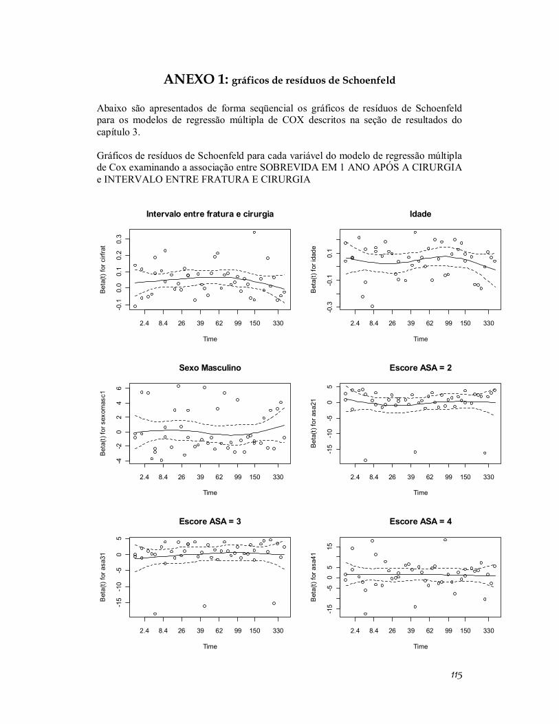
115
ANEXO 1: gráficos de resíduos de Schoenfeld
Abaixo são apresentados de forma seqüencial os gráficos de resíduos de Schoenfeld para os modelos de regressão múltipla de COX descritos na seção de resultados do capítulo 3. Gráficos de resíduos de Schoenfeld para cada variável do modelo de regressão múltipla de Cox examinando a associação entre SOBREVIDA EM 1 ANO APÓS A CIRURGIA e INTERVALO ENTRE FRATURA E CIRURGIA
Intervalo entre fratura e cirurgia
Time
Beta
(t) fo
r cirf
rat
2.4 8.4 26 39 62 99 150 330
-0.1
0.0
0.1
0.2
0.3
Idade
Time
Bet
a(t)
for i
dade
2.4 8.4 26 39 62 99 150 330-0
.3-0
.10.
1
Sexo Masculino
Time
Beta
(t) fo
r sex
omas
c1
2.4 8.4 26 39 62 99 150 330
-4-2
02
46
Escore ASA = 2
Time
Beta
(t) fo
r asa
21
2.4 8.4 26 39 62 99 150 330
-15
-10
-50
5
Escore ASA = 3
Time
Bet
a(t)
for a
sa31
2.4 8.4 26 39 62 99 150 330
-15
-10
-50
5
Escore ASA = 4
Time
Bet
a(t)
for a
sa41
2.4 8.4 26 39 62 99 150 330
-15
-50
515
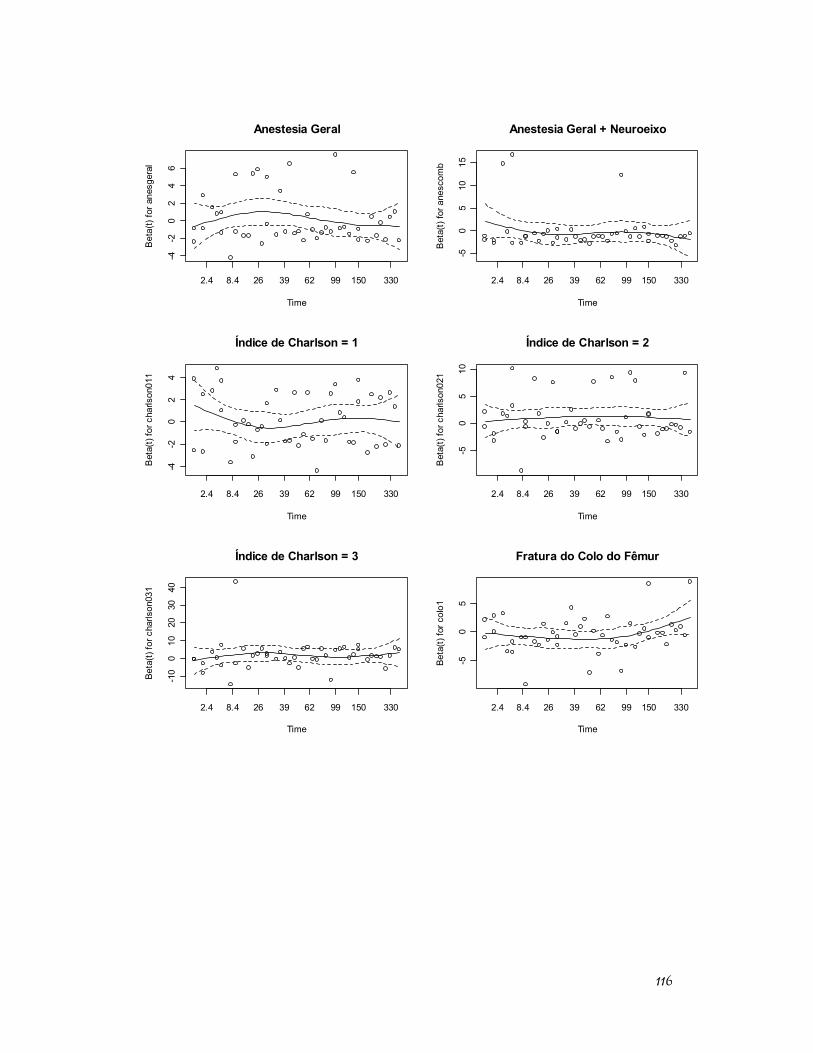
116
Anestesia Geral
Time
Bet
a(t)
for a
nesg
eral
2.4 8.4 26 39 62 99 150 330
-4-2
02
46
Anestesia Geral + Neuroeixo
Time
Bet
a(t)
for a
nesc
omb
2.4 8.4 26 39 62 99 150 330
-50
510
15
Índice de Charlson = 1
Time
Bet
a(t)
for c
harls
on01
1
2.4 8.4 26 39 62 99 150 330
-4-2
02
4
Índice de Charlson = 2
Time
Bet
a(t)
for c
harls
on02
1
2.4 8.4 26 39 62 99 150 330
-50
510
Índice de Charlson = 3
Time
Beta
(t) fo
r cha
rlson
031
2.4 8.4 26 39 62 99 150 330
-10
010
2030
40
Fratura do Colo do Fêmur
Time
Beta
(t) fo
r col
o1
2.4 8.4 26 39 62 99 150 330
-50
5
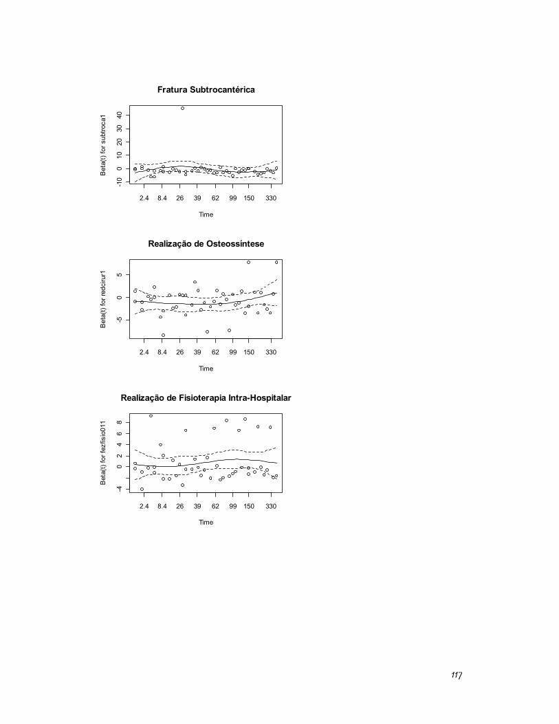
117
Fratura Subtrocantérica
Time
Bet
a(t)
for s
ubtro
ca1
2.4 8.4 26 39 62 99 150 330
-10
010
2030
40
Realização de Osteossíntese
Time
Bet
a(t)
for r
edci
rur1
2.4 8.4 26 39 62 99 150 330
-50
5
Realização de Fisioterapia Intra-Hospitalar
Time
Bet
a(t)
for f
ezfis
io01
1
2.4 8.4 26 39 62 99 150 330
-40
24
68
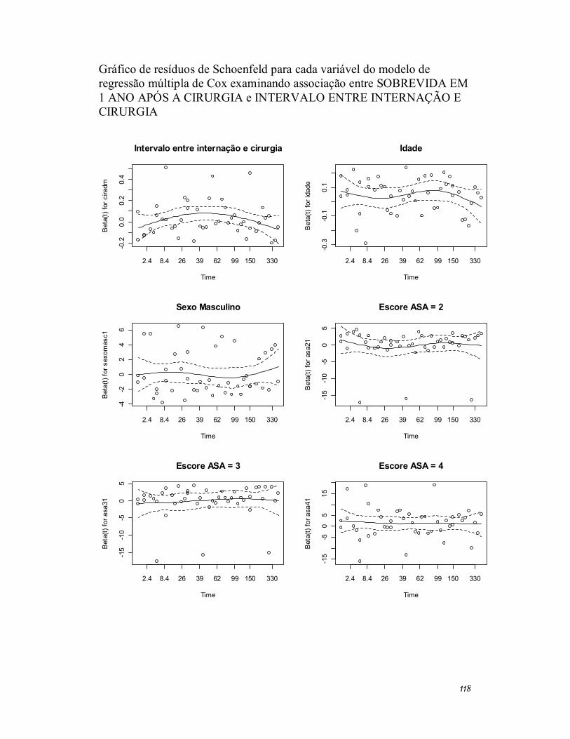
118
Gráfico de resíduos de Schoenfeld para cada variável do modelo de regressão múltipla de Cox examinando associação entre SOBREVIDA EM 1 ANO APÓS A CIRURGIA e INTERVALO ENTRE INTERNAÇÃO E CIRURGIA
Intervalo entre internação e cirurgia
Time
Bet
a(t)
for c
iradm
2.4 8.4 26 39 62 99 150 330
-0.2
0.0
0.2
0.4
Idade
Time
Bet
a(t)
for i
dade
2.4 8.4 26 39 62 99 150 330
-0.3
-0.1
0.1
Sexo Masculino
Time
Bet
a(t)
for s
exom
asc1
2.4 8.4 26 39 62 99 150 330
-4-2
02
46
Escore ASA = 2
Time
Bet
a(t)
for a
sa21
2.4 8.4 26 39 62 99 150 330
-15
-10
-50
5
Escore ASA = 3
Time
Bet
a(t)
for a
sa31
2.4 8.4 26 39 62 99 150 330
-15
-10
-50
5
Escore ASA = 4
Time
Bet
a(t)
for a
sa41
2.4 8.4 26 39 62 99 150 330
-15
-50
515
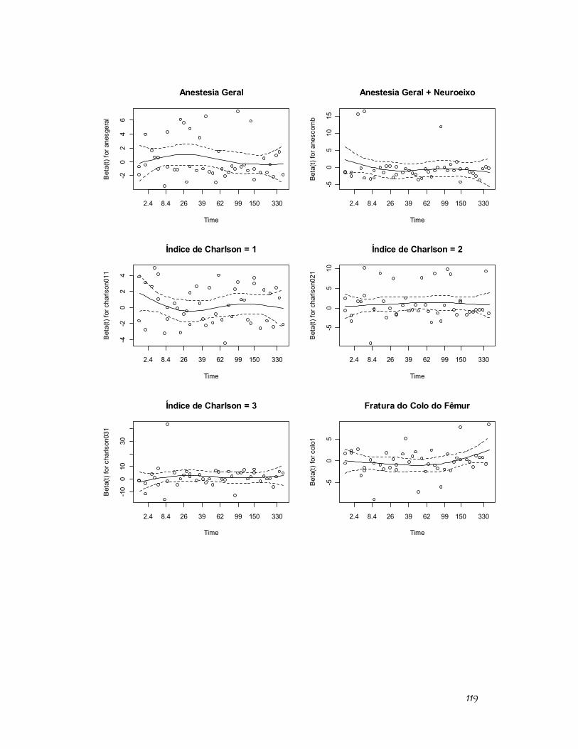
119
Anestesia Geral
Time
Bet
a(t)
for a
nesg
eral
2.4 8.4 26 39 62 99 150 330
-20
24
6
Anestesia Geral + Neuroeixo
Time
Bet
a(t)
for a
nesc
omb
2.4 8.4 26 39 62 99 150 330
-50
510
15
Índice de Charlson = 1
Time
Bet
a(t)
for c
harls
on01
1
2.4 8.4 26 39 62 99 150 330
-4-2
02
4
Índice de Charlson = 2
Time
Bet
a(t)
for c
harls
on02
1
2.4 8.4 26 39 62 99 150 330
-50
510
Índice de Charlson = 3
Time
Bet
a(t)
for c
harls
on03
1
2.4 8.4 26 39 62 99 150 330
-10
010
30
Fratura do Colo do Fêmur
Time
Bet
a(t)
for c
olo1
2.4 8.4 26 39 62 99 150 330
-50
5
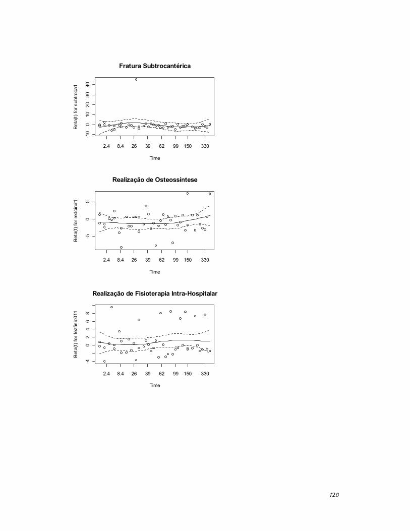
120
Fratura Subtrocantérica
Time
Bet
a(t)
for s
ubtro
ca1
2.4 8.4 26 39 62 99 150 330
-10
010
2030
40
Realização de Osteossíntese
Time
Bet
a(t)
for r
edci
rur1
2.4 8.4 26 39 62 99 150 330
-50
5
Realização de Fisioterapia Intra-Hospitalar
Time
Bet
a(t)
for f
ezfis
io01
1
2.4 8.4 26 39 62 99 150 330
-40
24
68
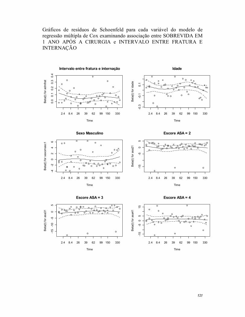
121
Gráficos de resíduos de Schoenfeld para cada variável do modelo de regressão múltipla de Cox examinando associação entre SOBREVIDA EM 1 ANO APÓS A CIRURGIA e INTERVALO ENTRE FRATURA E INTERNAÇÃO
Intervalo entre fratura e internação
Time
Bet
a(t)
for a
dmfra
t
2.4 8.4 26 39 62 99 150 330
0.0
0.1
0.2
0.3
0.4
Idade
Time
Bet
a(t)
for i
dade
2.4 8.4 26 39 62 99 150 330
-0.3
-0.1
0.1
Sexo Masculino
Time
Bet
a(t)
for s
exom
asc1
2.4 8.4 26 39 62 99 150 330
-4-2
02
46
Escore ASA = 2
Time
Bet
a(t)
for a
sa21
2.4 8.4 26 39 62 99 150 330
-15
-50
5
Escore ASA = 3
Time
Bet
a(t)
for a
sa31
2.4 8.4 26 39 62 99 150 330
-15
-10
-50
5
Escore ASA = 4
Time
Bet
a(t)
for a
sa41
2.4 8.4 26 39 62 99 150 330
-15
-50
515
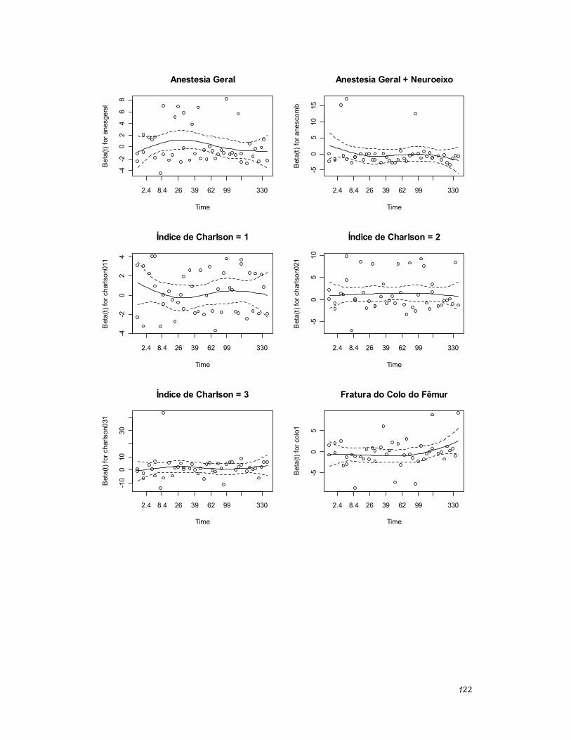
122
Anestesia Geral
Time
Bet
a(t)
for a
nesg
eral
2.4 8.4 26 39 62 99 330
-4-2
02
46
8
Anestesia Geral + Neuroeixo
Time
Bet
a(t)
for a
nesc
omb
2.4 8.4 26 39 62 99 330
-50
510
15
Índice de Charlson = 1
Time
Bet
a(t)
for c
harls
on01
1
2.4 8.4 26 39 62 99 330
-4-2
02
4
Índice de Charlson = 2
Time
Bet
a(t)
for c
harls
on02
1
2.4 8.4 26 39 62 99 330
-50
510
Índice de Charlson = 3
Time
Bet
a(t)
for c
harls
on03
1
2.4 8.4 26 39 62 99 330
-10
010
30
Fratura do Colo do Fêmur
Time
Bet
a(t)
for c
olo1
2.4 8.4 26 39 62 99 330
-50
5
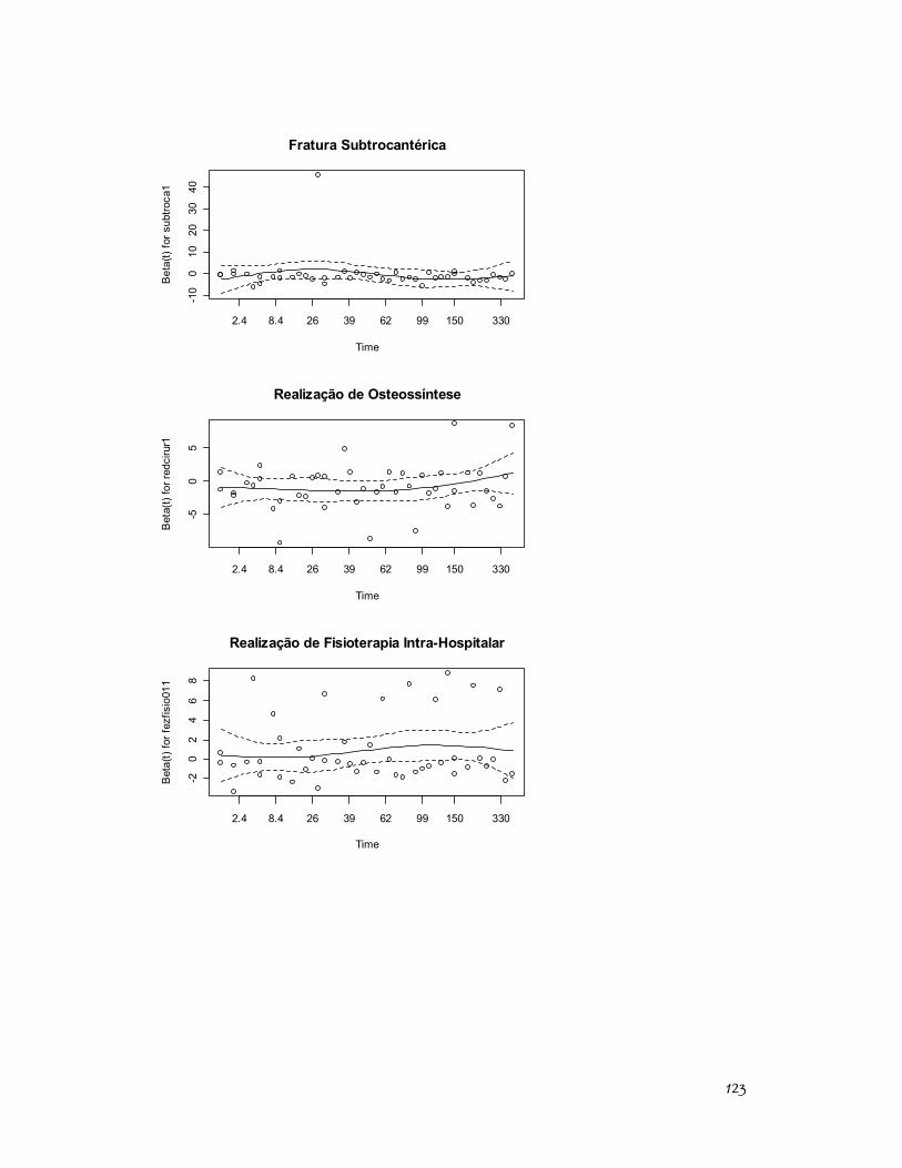
123
Fratura Subtrocantérica
Time
Bet
a(t)
for s
ubtro
ca1
2.4 8.4 26 39 62 99 150 330
-10
010
2030
40
Realização de Osteossíntese
Time
Bet
a(t)
for r
edci
rur1
2.4 8.4 26 39 62 99 150 330
-50
5
Realização de Fisioterapia Intra-Hospitalar
Time
Bet
a(t)
for f
ezfis
io01
1
2.4 8.4 26 39 62 99 150 330
-20
24
68
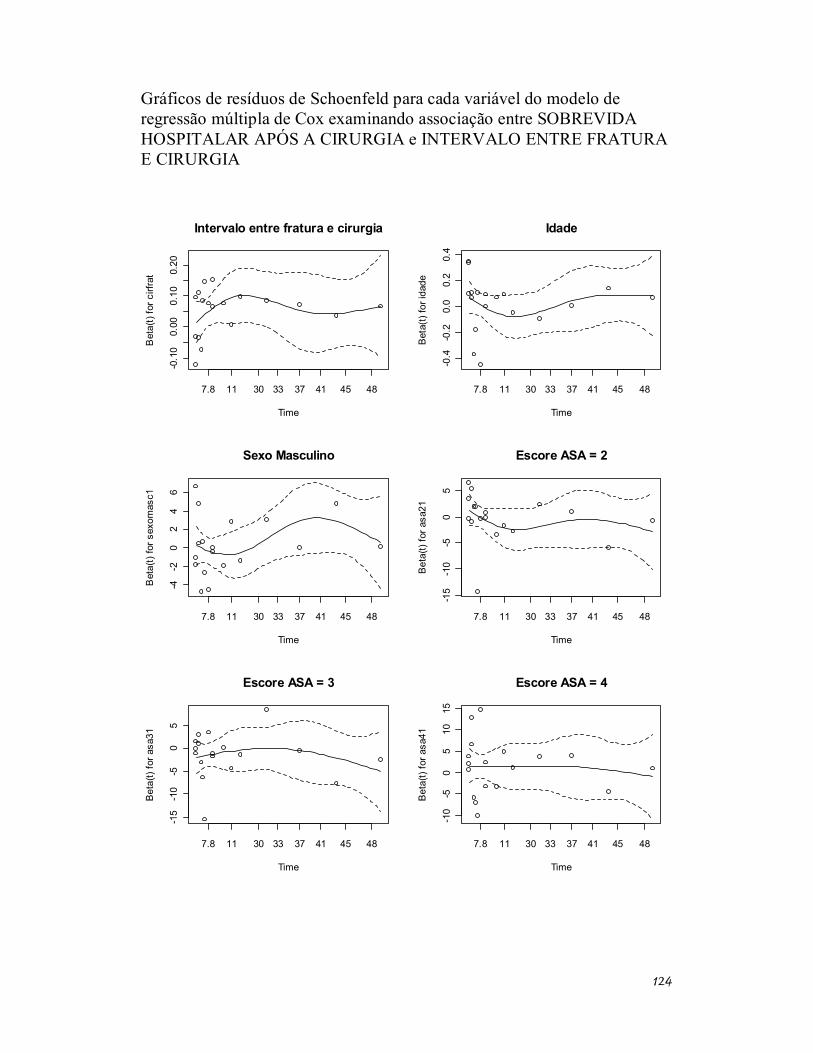
124
Gráficos de resíduos de Schoenfeld para cada variável do modelo de regressão múltipla de Cox examinando associação entre SOBREVIDA HOSPITALAR APÓS A CIRURGIA e INTERVALO ENTRE FRATURA E CIRURGIA
Intervalo entre fratura e cirurgia
Time
Bet
a(t)
for c
irfra
t
7.8 11 30 33 37 41 45 48
-0.1
00.
000.
100.
20
Idade
TimeB
eta(
t) fo
r ida
de
7.8 11 30 33 37 41 45 48
-0.4
-0.2
0.0
0.2
0.4
Sexo Masculino
Time
Bet
a(t)
for s
exom
asc1
7.8 11 30 33 37 41 45 48
-4-2
02
46
Escore ASA = 2
Time
Bet
a(t)
for a
sa21
7.8 11 30 33 37 41 45 48
-15
-10
-50
5
Escore ASA = 3
Time
Bet
a(t)
for a
sa31
7.8 11 30 33 37 41 45 48
-15
-10
-50
5
Escore ASA = 4
Time
Bet
a(t)
for a
sa41
7.8 11 30 33 37 41 45 48
-10
-50
510
15
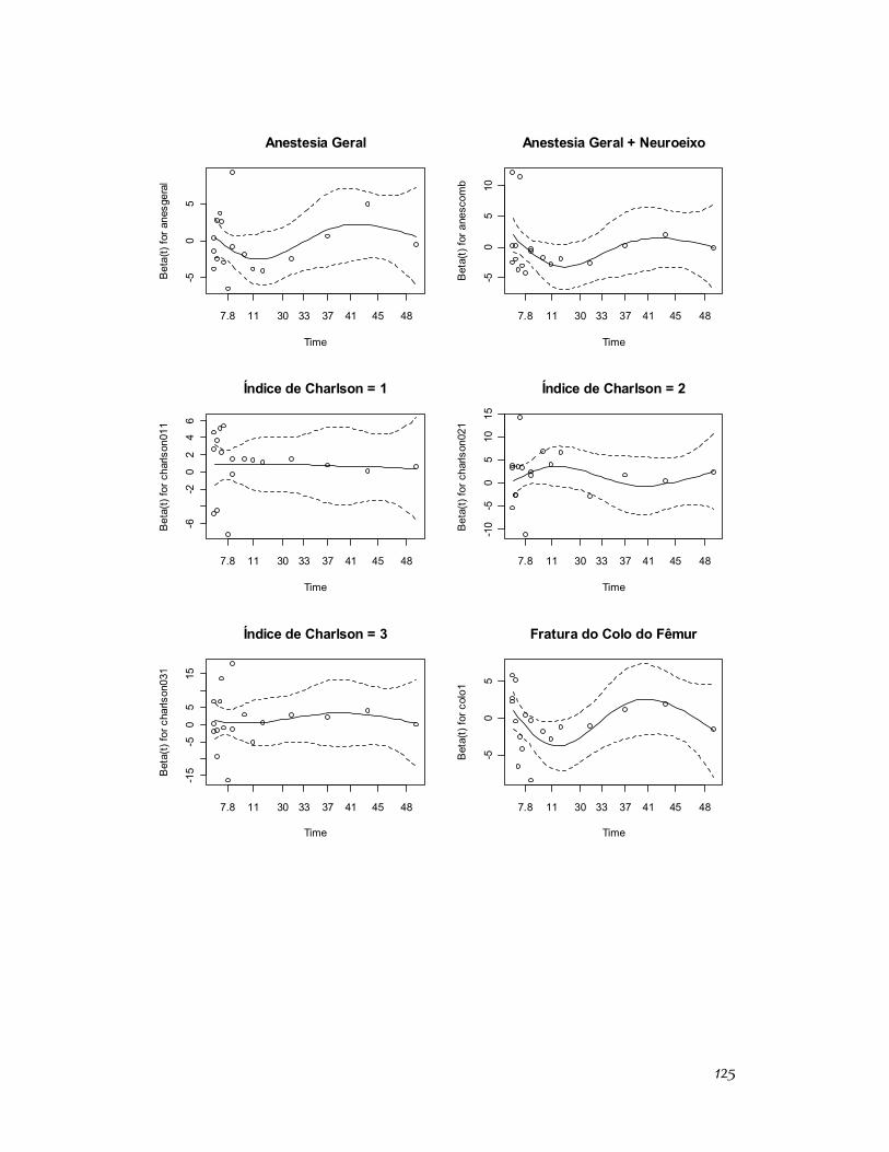
125
Anestesia Geral
Time
Bet
a(t)
for a
nesg
eral
7.8 11 30 33 37 41 45 48
-50
5
Anestesia Geral + Neuroeixo
Time
Bet
a(t)
for a
nesc
omb
7.8 11 30 33 37 41 45 48
-50
510
Índice de Charlson = 1
Time
Bet
a(t)
for c
harls
on01
1
7.8 11 30 33 37 41 45 48
-6-2
02
46
Índice de Charlson = 2
Time
Bet
a(t)
for c
harls
on02
1
7.8 11 30 33 37 41 45 48
-10
-50
510
15
Índice de Charlson = 3
Time
Bet
a(t)
for c
harls
on03
1
7.8 11 30 33 37 41 45 48
-15
-50
515
Fratura do Colo do Fêmur
Time
Bet
a(t)
for c
olo1
7.8 11 30 33 37 41 45 48
-50
5
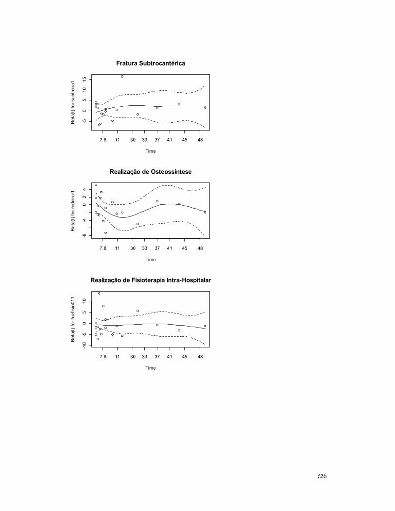
126
Fratura Subtrocantérica
Time
Bet
a(t)
for s
ubtro
ca1
7.8 11 30 33 37 41 45 48
-50
510
15
Realização de Osteossíntese
Time
Bet
a(t)
for r
edci
rur1
7.8 11 30 33 37 41 45 48
-8-4
02
4
Realização de Fisioterapia Intra-Hospitalar
Time
Bet
a(t)
for f
ezfis
io01
1
7.8 11 30 33 37 41 45 48
-10
-50
510
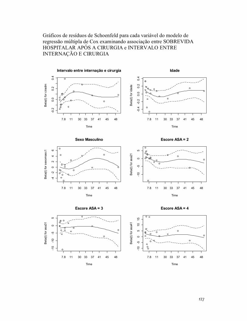
127
Gráficos de resíduos de Schoenfeld para cada variável do modelo de regressão múltipla de Cox examinando associação entre SOBREVIDA HOSPITALAR APÓS A CIRURGIA e INTERVALO ENTRE INTERNAÇÃO E CIRURGIA
Intervalo entre internação e cirurgia
Time
Bet
a(t)
for c
iradm
7.8 11 30 33 37 41 45 48
-0.2
0.0
0.2
0.4
Idade
TimeB
eta(
t) fo
r ida
de
7.8 11 30 33 37 41 45 48
-0.4
-0.2
0.0
0.2
0.4
Sexo Masculino
Time
Bet
a(t)
for s
exom
asc1
7.8 11 30 33 37 41 45 48
-4-2
02
46
Escore ASA = 2
Time
Bet
a(t)
for a
sa21
7.8 11 30 33 37 41 45 48
-10
-50
5
Escore ASA = 3
Time
Bet
a(t)
for a
sa31
7.8 11 30 33 37 41 45 48
-15
-10
-50
5
Escore ASA = 4
Time
Bet
a(t)
for a
sa41
7.8 11 30 33 37 41 45 48
-10
-50
510
15
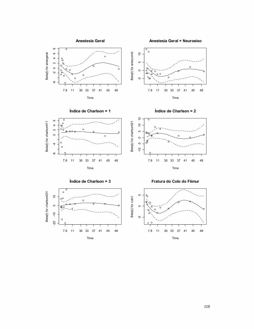
128
Anestesia Geral
Time
Bet
a(t)
for a
nesg
eral
7.8 11 30 33 37 41 45 48
-6-2
02
46
8
Anestesia Geral + Neuroeixo
Time
Bet
a(t)
for a
nesc
omb
7.8 11 30 33 37 41 45 48
-50
510
Índice de Charlson = 1
Time
Bet
a(t)
for c
harls
on01
1
7.8 11 30 33 37 41 45 48
-8-4
02
46
Índice de Charlson = 2
Time
Bet
a(t)
for c
harls
on02
1
7.8 11 30 33 37 41 45 48
-10
-50
510
15
Índice de Charlson = 3
Time
Bet
a(t)
for c
harls
on03
1
7.8 11 30 33 37 41 45 48
-20
-10
010
Fratura do Colo do Fêmur
Time
Bet
a(t)
for c
olo1
7.8 11 30 33 37 41 45 48
-50
5
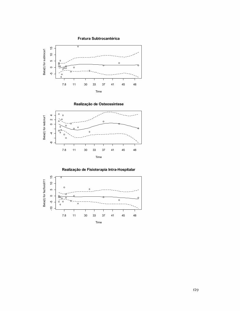
129
Fratura Subtrocantérica
Time
Bet
a(t)
for s
ubtro
ca1
7.8 11 30 33 37 41 45 48
-50
510
15
Realização de Osteossíntese
Time
Bet
a(t)
for r
edci
rur1
7.8 11 30 33 37 41 45 48
-8-4
02
4
Realização de Fisioterapia Intra-Hospitalar
Time
Bet
a(t)
for f
ezfis
io01
1
7.8 11 30 33 37 41 45 48
-10
-50
510
15
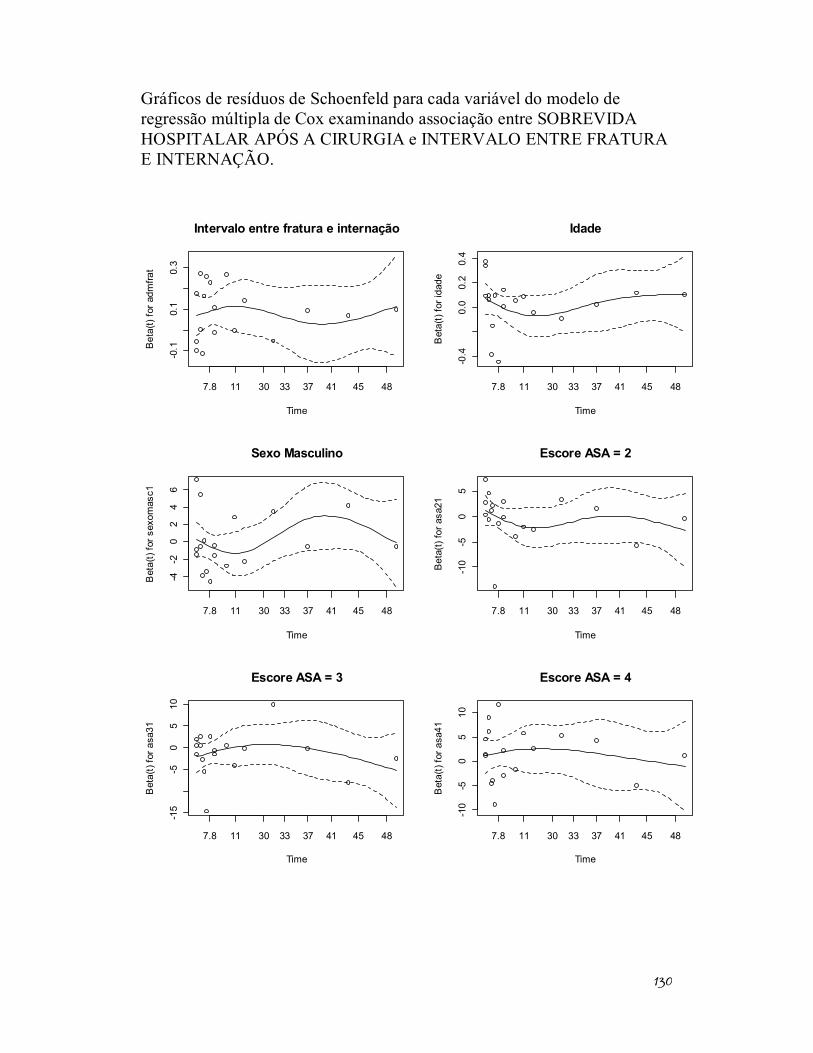
130
Gráficos de resíduos de Schoenfeld para cada variável do modelo de regressão múltipla de Cox examinando associação entre SOBREVIDA HOSPITALAR APÓS A CIRURGIA e INTERVALO ENTRE FRATURA E INTERNAÇÃO.
Intervalo entre fratura e internação
Time
Bet
a(t)
for a
dmfra
t
7.8 11 30 33 37 41 45 48
-0.1
0.1
0.3
Idade
Time
Bet
a(t)
for i
dade
7.8 11 30 33 37 41 45 48
-0.4
0.0
0.2
0.4
Sexo Masculino
Time
Bet
a(t)
for s
exom
asc1
7.8 11 30 33 37 41 45 48
-4-2
02
46
Escore ASA = 2
Time
Bet
a(t)
for a
sa21
7.8 11 30 33 37 41 45 48
-10
-50
5
Escore ASA = 3
Time
Bet
a(t)
for a
sa31
7.8 11 30 33 37 41 45 48
-15
-50
510
Escore ASA = 4
Time
Bet
a(t)
for a
sa41
7.8 11 30 33 37 41 45 48
-10
-50
510
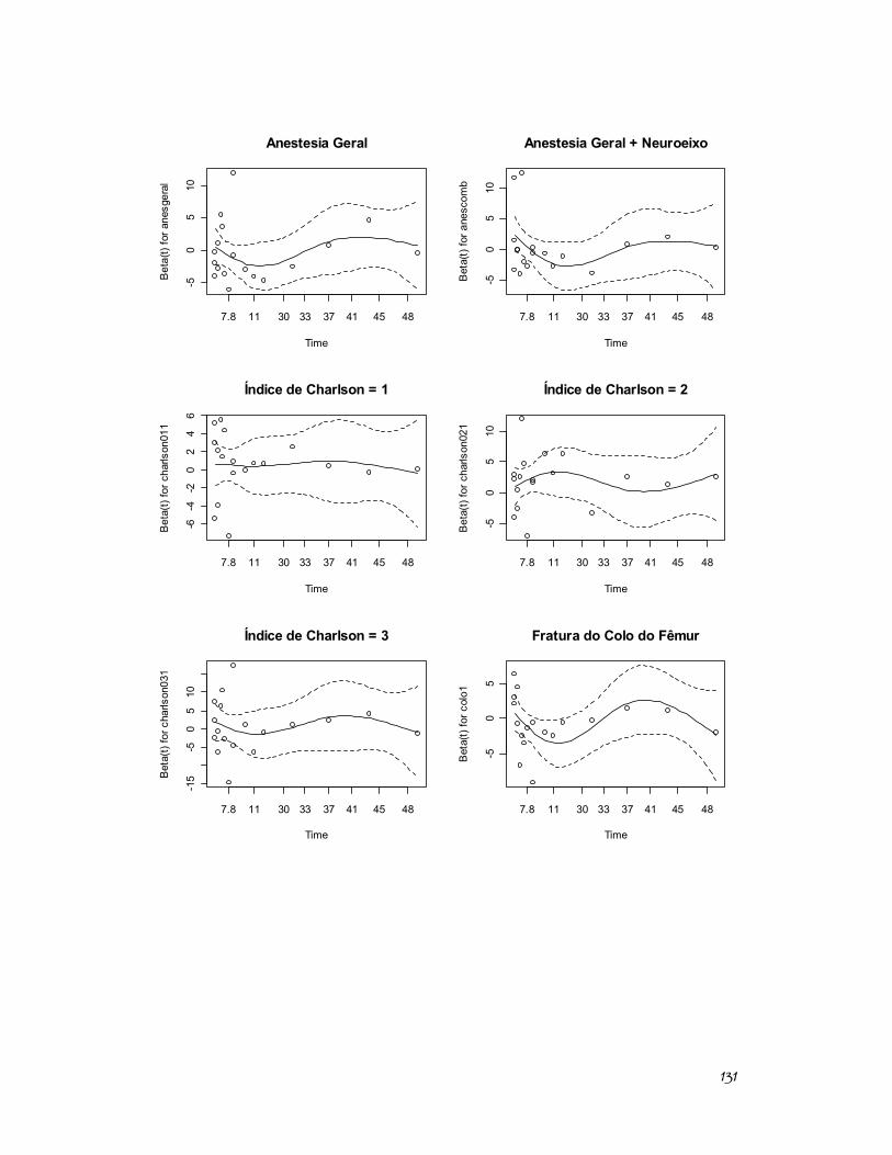
131
Anestesia Geral
Time
Bet
a(t)
for a
nesg
eral
7.8 11 30 33 37 41 45 48
-50
510
Anestesia Geral + Neuroeixo
Time
Bet
a(t)
for a
nesc
omb
7.8 11 30 33 37 41 45 48
-50
510
Índice de Charlson = 1
Time
Bet
a(t)
for c
harls
on01
1
7.8 11 30 33 37 41 45 48
-6-4
-20
24
6
Índice de Charlson = 2
Time
Bet
a(t)
for c
harls
on02
1
7.8 11 30 33 37 41 45 48
-50
510
Índice de Charlson = 3
Time
Bet
a(t)
for c
harls
on03
1
7.8 11 30 33 37 41 45 48
-15
-50
510
Fratura do Colo do Fêmur
Time
Bet
a(t)
for c
olo1
7.8 11 30 33 37 41 45 48
-50
5
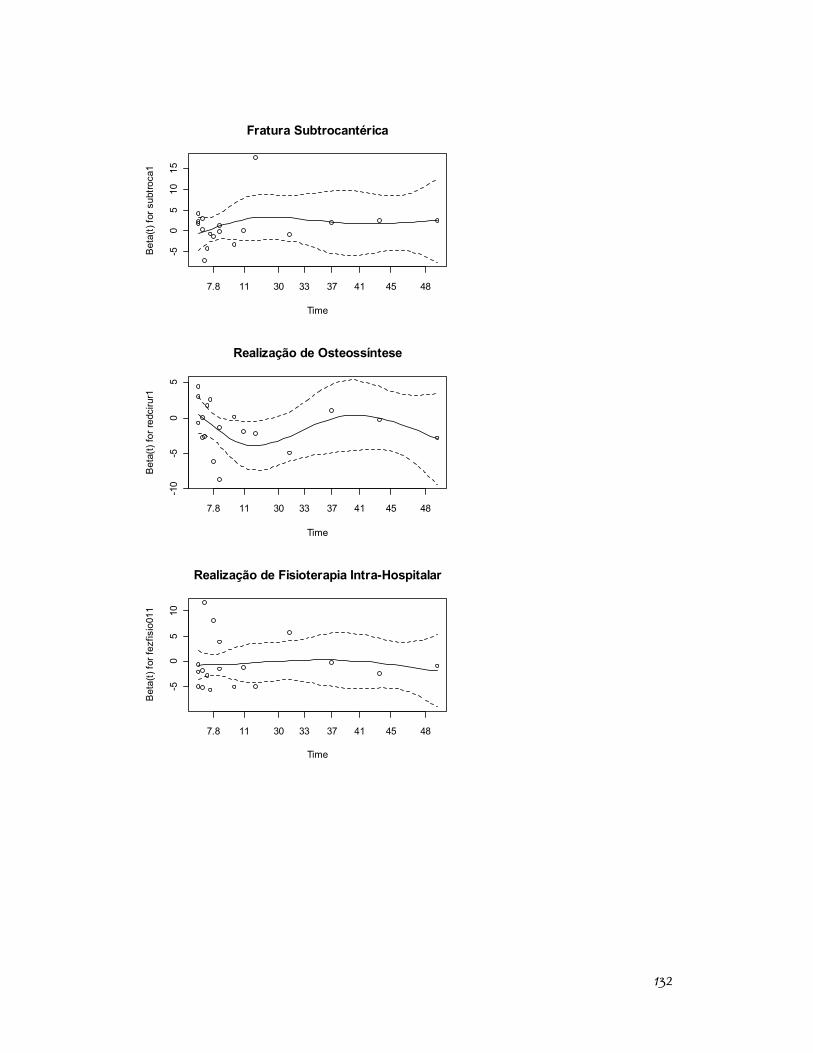
132
Fratura Subtrocantérica
Time
Bet
a(t)
for s
ubtro
ca1
7.8 11 30 33 37 41 45 48
-50
510
15
Realização de Osteossíntese
Time
Bet
a(t)
for r
edci
rur1
7.8 11 30 33 37 41 45 48
-10
-50
5
Realização de Fisioterapia Intra-Hospitalar
Time
Bet
a(t)
for f
ezfis
io01
1
7.8 11 30 33 37 41 45 48
-50
510
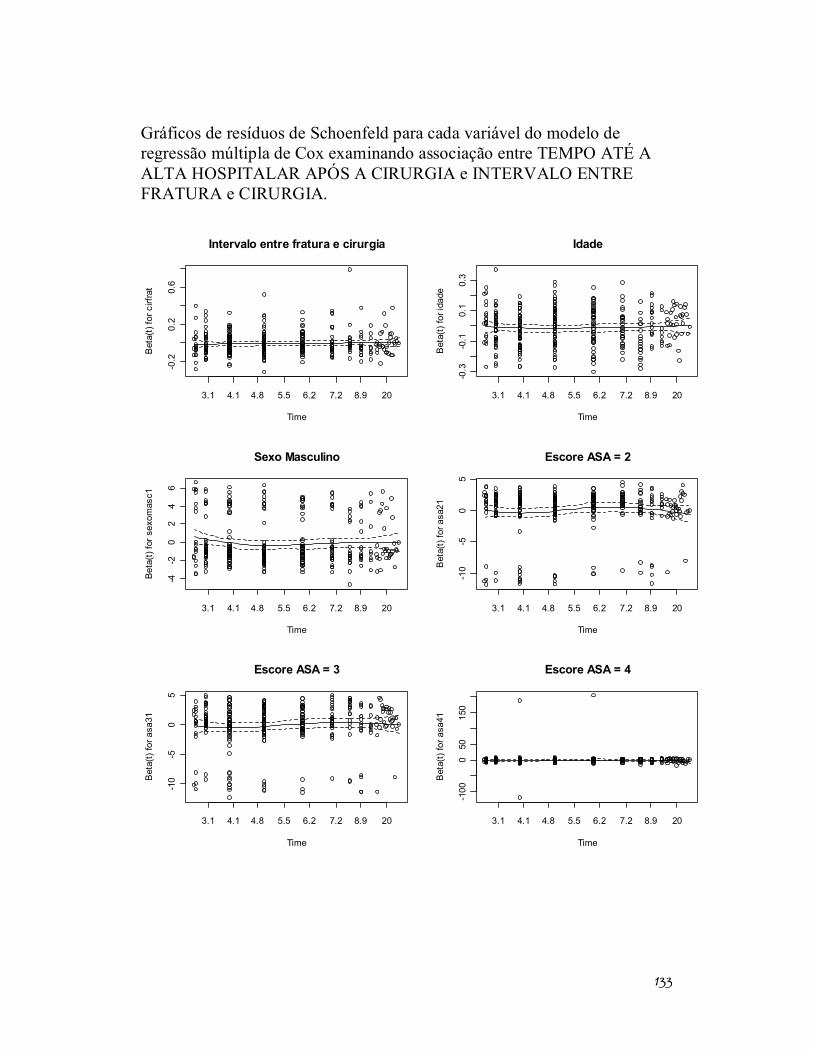
133
Gráficos de resíduos de Schoenfeld para cada variável do modelo de regressão múltipla de Cox examinando associação entre TEMPO ATÉ A ALTA HOSPITALAR APÓS A CIRURGIA e INTERVALO ENTRE FRATURA e CIRURGIA.
Intervalo entre fratura e cirurgia
Time
Bet
a(t)
for c
irfra
t
3.1 4.1 4.8 5.5 6.2 7.2 8.9 20
-0.2
0.2
0.6
Idade
Time
Bet
a(t)
for i
dade
3.1 4.1 4.8 5.5 6.2 7.2 8.9 20
-0.3
-0.1
0.1
0.3
Sexo Masculino
Time
Beta
(t) fo
r sex
omas
c1
3.1 4.1 4.8 5.5 6.2 7.2 8.9 20
-4-2
02
46
Escore ASA = 2
Time
Bet
a(t)
for a
sa21
3.1 4.1 4.8 5.5 6.2 7.2 8.9 20
-10
-50
5
Escore ASA = 3
Time
Bet
a(t)
for a
sa31
3.1 4.1 4.8 5.5 6.2 7.2 8.9 20
-10
-50
5
Escore ASA = 4
Time
Bet
a(t)
for a
sa41
3.1 4.1 4.8 5.5 6.2 7.2 8.9 20
-100
050
150
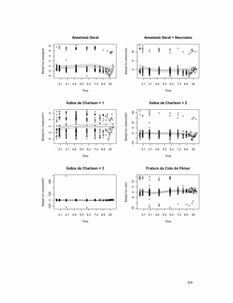
134
Anestesia Geral
Time
Bet
a(t)
for a
nesg
eral
3.1 4.1 4.8 5.5 6.2 7.2 8.9 20
-4-2
02
46
8
Anestesia Geral + Neuroeixo
Time
Bet
a(t)
for a
nesc
omb
3.1 4.1 4.8 5.5 6.2 7.2 8.9 20
05
10
Índice de Charlson = 1
Time
Bet
a(t)
for c
harls
on01
1
3.1 4.1 4.8 5.5 6.2 7.2 8.9 20
-4-2
02
4
Índice de Charlson = 2
Time
Bet
a(t)
for c
harls
on02
1
3.1 4.1 4.8 5.5 6.2 7.2 8.9 20
-10
05
1020
Índice de Charlson = 3
Time
Bet
a(t)
for c
harls
on03
1
3.1 4.1 4.8 5.5 6.2 7.2 8.9 20
-100
010
030
0
Fratura do Colo do Fêmur
Time
Bet
a(t)
for c
olo1
3.1 4.1 4.8 5.5 6.2 7.2 8.9 20
-15
-50
510
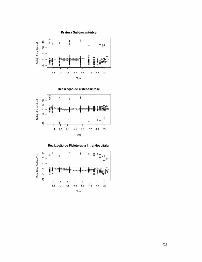
135
Fratura Subtrocantérica
Time
Bet
a(t)
for s
ubtro
ca1
3.1 4.1 4.8 5.5 6.2 7.2 8.9 20
-50
510
15
Realização de Osteossíntese
Time
Bet
a(t)
for r
edci
rur1
3.1 4.1 4.8 5.5 6.2 7.2 8.9 20
-15
-50
510
Realização de Fisioterapia Intra-Hospitalar
Time
Bet
a(t)
for f
ezfis
io01
1
3.1 4.1 4.8 5.5 6.2 7.2 8.9 20
-10
-50
510
15
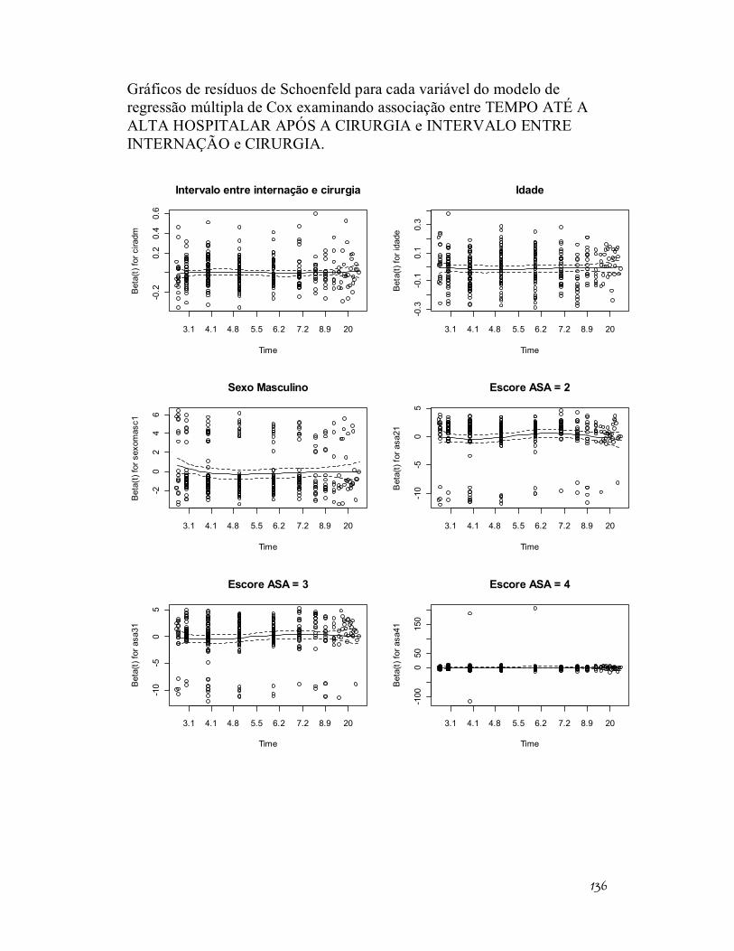
136
Gráficos de resíduos de Schoenfeld para cada variável do modelo de regressão múltipla de Cox examinando associação entre TEMPO ATÉ A ALTA HOSPITALAR APÓS A CIRURGIA e INTERVALO ENTRE INTERNAÇÃO e CIRURGIA.
Intervalo entre internação e cirurgia
Time
Bet
a(t)
for c
iradm
3.1 4.1 4.8 5.5 6.2 7.2 8.9 20
-0.2
0.2
0.4
0.6
Idade
Time
Bet
a(t)
for i
dade
3.1 4.1 4.8 5.5 6.2 7.2 8.9 20
-0.3
-0.1
0.1
0.3
Sexo Masculino
Time
Bet
a(t)
for s
exom
asc1
3.1 4.1 4.8 5.5 6.2 7.2 8.9 20
-20
24
6
Escore ASA = 2
Time
Bet
a(t)
for a
sa21
3.1 4.1 4.8 5.5 6.2 7.2 8.9 20
-10
-50
5
Escore ASA = 3
Time
Bet
a(t)
for a
sa31
3.1 4.1 4.8 5.5 6.2 7.2 8.9 20
-10
-50
5
Escore ASA = 4
Time
Bet
a(t)
for a
sa41
3.1 4.1 4.8 5.5 6.2 7.2 8.9 20
-100
050
150
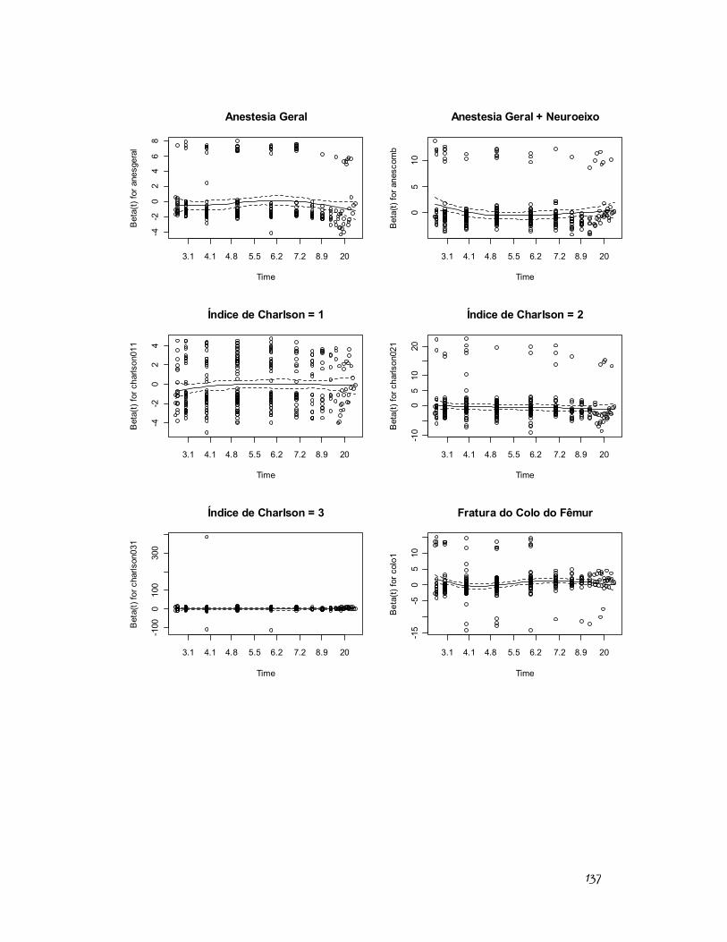
137
Anestesia Geral
Time
Bet
a(t)
for a
nesg
eral
3.1 4.1 4.8 5.5 6.2 7.2 8.9 20
-4-2
02
46
8
Anestesia Geral + Neuroeixo
Time
Bet
a(t)
for a
nesc
omb
3.1 4.1 4.8 5.5 6.2 7.2 8.9 20
05
10
Índice de Charlson = 1
Time
Bet
a(t)
for c
harls
on01
1
3.1 4.1 4.8 5.5 6.2 7.2 8.9 20
-4-2
02
4
Índice de Charlson = 2
Time
Bet
a(t)
for c
harls
on02
1
3.1 4.1 4.8 5.5 6.2 7.2 8.9 20
-10
05
1020
Índice de Charlson = 3
Time
Bet
a(t)
for c
harls
on03
1
3.1 4.1 4.8 5.5 6.2 7.2 8.9 20
-100
010
030
0
Fratura do Colo do Fêmur
Time
Bet
a(t)
for c
olo1
3.1 4.1 4.8 5.5 6.2 7.2 8.9 20
-15
-50
510
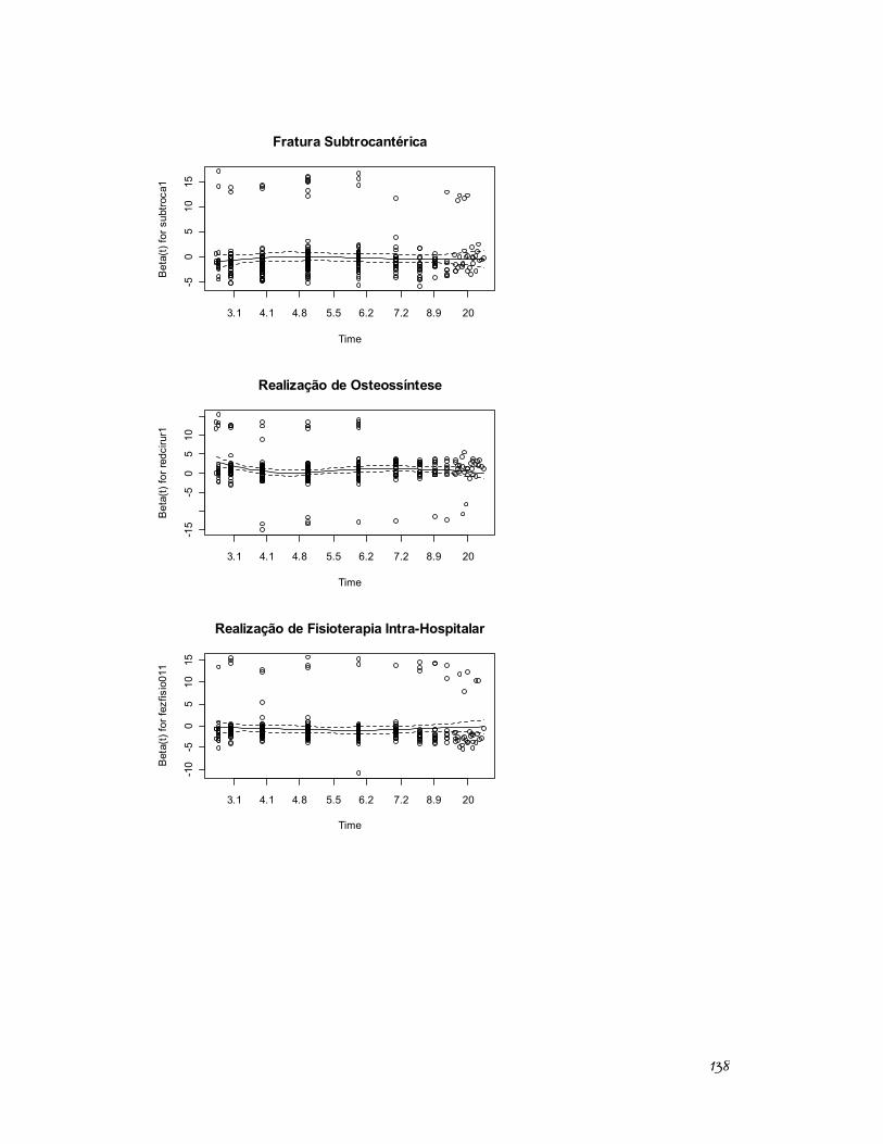
138
Fratura Subtrocantérica
Time
Bet
a(t)
for s
ubtro
ca1
3.1 4.1 4.8 5.5 6.2 7.2 8.9 20
-50
510
15
Realização de Osteossíntese
Time
Bet
a(t)
for r
edci
rur1
3.1 4.1 4.8 5.5 6.2 7.2 8.9 20
-15
-50
510
Realização de Fisioterapia Intra-Hospitalar
Time
Bet
a(t)
for f
ezfis
io01
1
3.1 4.1 4.8 5.5 6.2 7.2 8.9 20
-10
-50
510
15
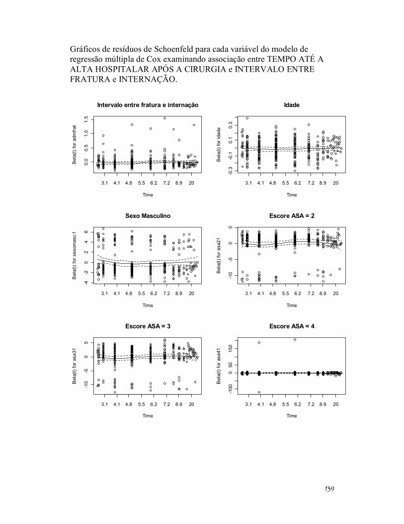
139
Gráficos de resíduos de Schoenfeld para cada variável do modelo de regressão múltipla de Cox examinando associação entre TEMPO ATÉ A ALTA HOSPITALAR APÓS A CIRURGIA e INTERVALO ENTRE FRATURA e INTERNAÇÃO.
Intervalo entre fratura e internação
Time
Bet
a(t)
for a
dmfra
t
3.1 4.1 4.8 5.5 6.2 7.2 8.9 20
0.0
0.5
1.0
1.5
Idade
Time
Bet
a(t)
for i
dade
3.1 4.1 4.8 5.5 6.2 7.2 8.9 20
-0.3
-0.1
0.1
0.3
Sexo Masculino
Time
Bet
a(t)
for s
exom
asc1
3.1 4.1 4.8 5.5 6.2 7.2 8.9 20
-4-2
02
46
Escore ASA = 2
Time
Bet
a(t)
for a
sa21
3.1 4.1 4.8 5.5 6.2 7.2 8.9 20
-10
-50
5
Escore ASA = 3
Time
Bet
a(t)
for a
sa31
3.1 4.1 4.8 5.5 6.2 7.2 8.9 20
-10
-50
5
Escore ASA = 4
Time
Bet
a(t)
for a
sa41
3.1 4.1 4.8 5.5 6.2 7.2 8.9 20
-100
050
150
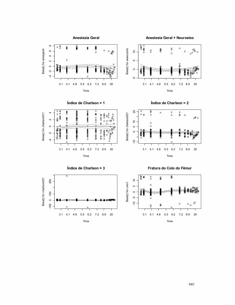
140
Anestesia Geral
Time
Bet
a(t)
for a
nesg
eral
3.1 4.1 4.8 5.5 6.2 7.2 8.9 20
-4-2
02
46
8
Anestesia Geral + Neuroeixo
Time
Bet
a(t)
for a
nesc
omb
3.1 4.1 4.8 5.5 6.2 7.2 8.9 20
-50
510
Índice de Charlson = 1
Time
Bet
a(t)
for c
harls
on01
1
3.1 4.1 4.8 5.5 6.2 7.2 8.9 20
-4-2
02
4
Índice de Charlson = 2
Time
Bet
a(t)
for c
harls
on02
1
3.1 4.1 4.8 5.5 6.2 7.2 8.9 20
-10
05
1020
Índice de Charlson = 3
Time
Bet
a(t)
for c
harls
on03
1
3.1 4.1 4.8 5.5 6.2 7.2 8.9 20
-100
010
030
0
Fratura do Colo do Fêmur
Time
Bet
a(t)
for c
olo1
3.1 4.1 4.8 5.5 6.2 7.2 8.9 20
-10
-50
510
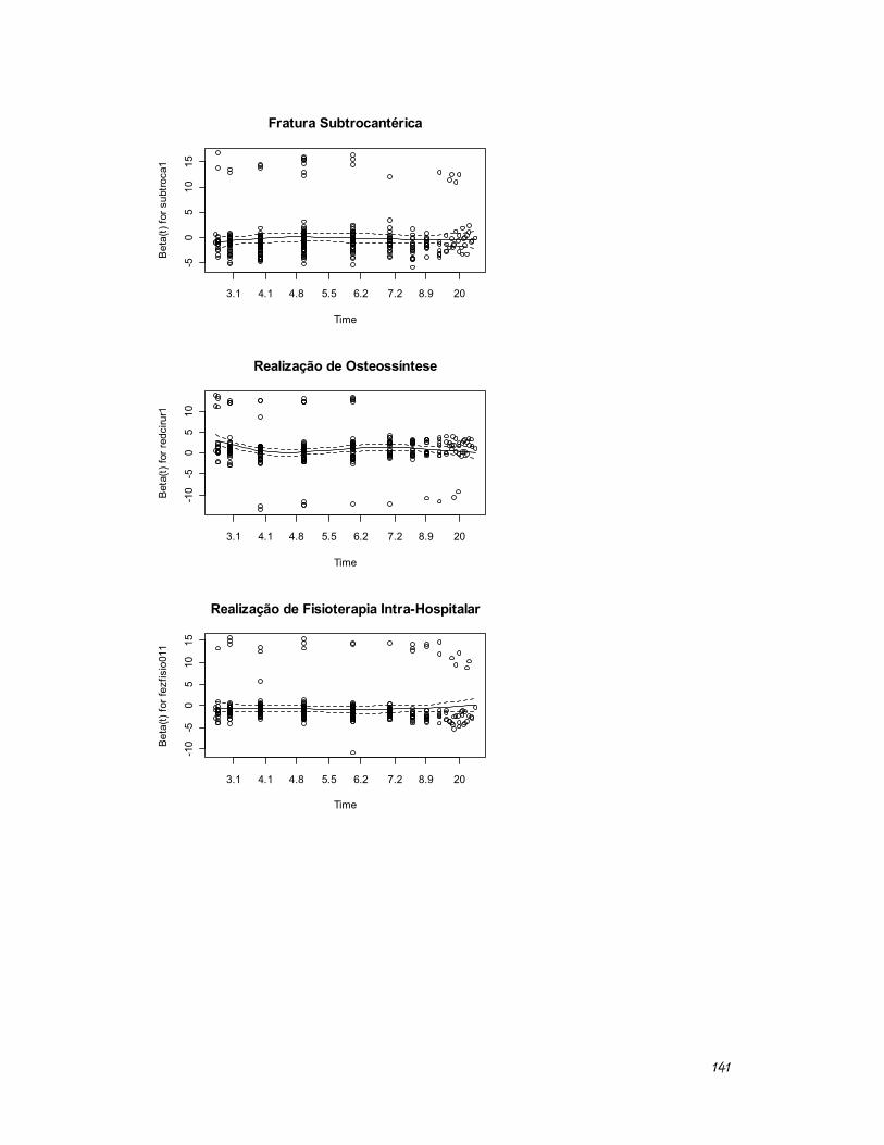
141
Fratura Subtrocantérica
Time
Bet
a(t)
for s
ubtro
ca1
3.1 4.1 4.8 5.5 6.2 7.2 8.9 20
-50
510
15
Realização de Osteossíntese
Time
Bet
a(t)
for r
edci
rur1
3.1 4.1 4.8 5.5 6.2 7.2 8.9 20
-10
-50
510
Realização de Fisioterapia Intra-Hospitalar
Time
Bet
a(t)
for f
ezfis
io01
1
3.1 4.1 4.8 5.5 6.2 7.2 8.9 20
-10
-50
510
15
143
ANEXO 2: script de programação utilizado
Script de programação utilizado para análise dos dados através do Software R: # Adequando o banco de dados e analisando suas variáveis # Carregando pacote "foreign" para leitura de banco de dados tipo ".dta" (stata) library(foreign) frat = read.dta("frathu8CSP.dta") # Carregando pagote "car" library(car) # Selecionando pacientes com 60 anos ou mais e excluindo pacientes com # tipo de fratura não definido frat1 = frat[frat$idade>=60,] frat1 = frat1[frat1$tipofrat != 4,] # Adequando o banco de dados frat1$sexo= as.factor(frat1$sexo) frat1$morario = as.factor(frat1$morario) frat1$causafra = as.factor(frat1$causafra) frat1$tipofrat = as.factor(frat1$tipofrat) frat1$tipociru= as.factor(frat1$tipociru) frat1$tipoanes= as.factor(frat1$tipoanes) frat1$anticoag= as.factor(frat1$anticoag) frat1$antib = as.factor(frat1$antib) frat1$fezfisio= as.factor(frat1$fezfisio) frat1$qtdcomoF=as.factor(frat1$qtdcomo) frat1$uso_cti= as.factor(frat1$uso_cti) frat1$asafinal = as.factor(frat1$asafinal) frat1$compmeno = as.factor(frat1$compmeno) frat1$compmaio = as.factor(frat1$compmaio) frat1$compciru = as.factor(frat1$compciru) frat1$compment = as.factor(frat1$compment) frat1$asacomb = as.factor(frat1$asacomb) frat1$confment = as.factor(frat1$confment) frat1$obstruca = as.factor(frat1$obstruca) frat1$pneumoni = as.factor(frat1$pneumoni) frat1$infarto = as.factor(frat1$infarto) frat1$hemodige = as.factor (frat1$hemodige) frat1$edema = as.factor(frat1$edema) frat1$estcivil = as.factor(frat1$estcivil) frat1$fez_antib = as.factor(frat1$fez_antib) frat1$fez_antib2 = as.factor(frat1$fez_antib2) frat1$escolar = as.factor(frat1$escolar) frat1$escolar[frat1$escolar == 9] = NA frat1$renda[frat1$renda >900] = NA frat1$cohabita = as.factor(frat1$cohabita) frat1$funcao = as.factor(frat1$funcao) frat1$tipofrat = as.factor(frat1$tipofrat) frat1$asafinal = as.factor(frat1$asafinal) frat1$asa1= as.factor(frat1$asa1) frat1$asa2= as.factor(frat1$asa2) frat1$asa3= as.factor(frat1$asa3) frat1$asa4= as.factor(frat1$asa4) frat1$asa= as.factor(frat1$asa) frat1$clinasa= as.factor(frat1$clinasa) frat1$charlson = as.factor(frat1$charlson) frat1$qtcomogr = as.factor(frat1$qtcomogr)

144
frat1$como = as.factor(frat1$como) frat1$como01 = as.factor(frat1$como01) frat1$como02 = as.factor(frat1$como02) frat1$como03 = as.factor(frat1$como03) frat1$como04 = as.factor(frat1$como04) frat1$como05 = as.factor(frat1$como05) frat1$como06 = as.factor(frat1$como06) frat1$como07 = as.factor(frat1$como07) frat1$como08 = as.factor(frat1$como08) frat1$como09 = as.factor(frat1$como09) frat1$escaras = as.factor(frat1$escaras) frat1$obito1 = as.factor(frat1$obito1) frat1$ob_hosp = as.factor(frat1$ob_hosp) frat1$ob_30dia = as.factor(frat1$ob_30dia) frat1$ob_90dia = as.factor(frat1$ob_90dia) frat1$ob_180di = as.factor(frat1$ob_180di) frat1$ob_1ano = as.factor(frat1$ob_1ano) frat1$destinos = as.factor(frat1$destinos) frat1$readmiss = as.factor(frat1$readmiss) frat1$escara12 = as.factor(frat1$escara12) frat1$fez_con_mental = as.factor(frat1$fez_con_mental) frat1$comp_infcir = as.factor(frat1$comp_infcir) frat1$qtdcomo = as.factor(frat1$qtdcomo) frat1$compciru = as.factor(frat1$compciru) frat1$qqcompl = as.factor(frat1$qqcompl) frat1$comp_cment = as.factor(frat1$comp_cment) frat1$comp_outr = as.factor(frat1$comp_outr) frat1$comp_revis = as.factor(frat1$comp_revis) frat1$comp_desloc = as.factor(frat1$comp_desloc) frat1$sexomasc= as.factor(frat1$sexomasc) frat1$cominuti= as.factor(frat1$cominuti) frat1$protese = as.factor(frat1$protese) frat1$redcirur = as.factor(frat1$redcirur) frat1$cirfixa= as.factor(frat1$cirfixa) frat1$cirprot= as.factor(frat1$cirprot) frat1$intertro=as.factor(frat1$intertro) frat1$subtroca= as.factor(frat1$subtroca) frat1$colo=as.factor(frat1$colo) frat1$cidmaior = as.factor(frat1$cidmaior) frat1$comomaio = as.factor(frat1$comomaio) frat1$anticoag = as.factor(frat1$anticoag) frat1$obito = as.factor(frat1$obito) class(frat1$dataalta) class(frat1$datafrat) class(frat1$dataciru) class(frat1$dataprim) class(frat1$datasegu) class(frat1$data_obi) class(frat1$datafra1) class(frat1$dataadmi) frat1$dataadmi1 = as.Date.character(frat1$dataadmi, format="%m/%d/%Y") frat1$dataalta1 = as.Date.character(frat1$dataalta, format="%m/%d/%Y") frat1$datafrat1 = as.Date.character(frat1$datafra1, format="%m/%d/%Y") frat1$dataciru1 = as.Date.character(frat1$dataciru, format="%m/%d/%Y") frat1$dataprim1 = as.Date.character(frat1$dataprim, format="%m/%d/%Y") frat1$datasegu1 = as.Date.character(frat1$datasegu, format="%m/%d/%Y") frat1$data_obi1 = as.Date.character(frat1$data_obi, format="%m/%d/%Y") ## CORRIGINDO ALGUMAS POUCAS DATAS COM ERRO MANUALMENTE frat1$dataadmi1[157] = "1997-09-26" frat1$dataadmi1[296]= "2000-05-27" frat1$datafrat1[296]= "2000-05-27"
145
frat1$datafrat1[200]= "1995-08-18" frat1$datafrat1[184]= "1996-04-14" frat1$datafrat1[321]= "1999-03-28" frat1$dataadmi1[47]= "1995-05-25" frat1$dataadmi1[343]= "1995-10-27" frat1$datafrat1[297]= "1999-12-10" ## EXCLUINDO INDIVÍDUOS PORTADORES DE VALORES DUVIDOSOS PARA A DATA DA FRATURA, INTERNAÇÃO OU CIRURGIA frat1$id = 1:352 frat1 = subset(frat1, frat1$id != 47 & frat1$id != 157 & frat1$id != 171 & frat1$id != 184 & frat1$id != 200 & frat1$id != 296 & frat1$id != 297 & frat1$id != 321 & frat1$id != 343) ### OPTEI POR NÃO ALTERAR AS DATAS ABAIXO ## frat1$datafrat1[348] ## OPTEI POR NÃO ALTERAR, PORQUE ACHO QUE NÃO HOUVE ERRO DE DIGITAÇÃO. AS DATAS SÃO SEQUENCIAIS E OCORREM EM ANOS DIFERENTES DE MODO PLAUSÍVEL. ## frat1$datafrat1[202] ## OPTEI POR NÃO ALTERAR PORQUE O INTERVALO ENTRE A FRATURA E A INTERNAÇÃO ERA INFERIOR A 30 DIAS # frat1$datafrat1[30] = "1995-09-28" # frat1$datafrat1[42] = "1997-08-13" # frat1$datafrat1[299] = "2000-06-08" ## CRIANDO VARIÁVEIS MEDINDO OS INTERVALOS DE TEMPO DE INTERESSE frat1$deltafratciru1 = frat1$dataciru1-frat1$datafrat1 frat1$deltaadmiciru1 = frat1$dataciru1-frat1$dataadmi1 frat1$deltafratadmi1 = frat1$dataadmi1 - frat1$datafrat1 frat1$delta_obifrat = frat1$data_obi1-frat1$datafrat1 frat1$delta_altaadmi1 = frat1$dataalta1-frat1$dataadmi1 frat1$delta_altaciru1 = frat1$dataalta1-frat1$dataciru1 summary(frat1$deltafratciru1 ) summary(frat1$deltaadmiciru1 ) summary(frat1$deltafratadmi1 ) summary(frat1$delta_obifrat ) summary(frat1$delta_altaadmi1 ) summary(frat1$cirfrat) summary(frat1$ciradm) summary(frat1$admfrat) # SALVANDO AS VARIÁVEIS CIRFRAT, CIRADM e ADMFRA em variáveis antigas, pois é preciso corrigir os erros encontrados nas originais frat1$cirfrat = frat1$cirfratANTIGA frat1$ciradm = frat1$ciradmANTIGA frat1$admfrat = frat1$admfratANTIGA # SUBSTITUINDO AS VARIÁVEIS CIRFRAT, CIRADM e ADMFRA PELAS VARIÁVEIS DELTAFRATCIRU1, DELTAADMICIRU1, DELTAFRATADMI1 frat1$cirfrat = frat1$deltafratciru1 frat1$ciradm = frat1$deltaadmiciru1 frat1$admfrat = frat1$deltafratadmi1 ## DIVIDINDO A IDADE EM FAIXAS CATIDADE1 <- frat1$idade CATIDADE1[frat1$idade >= 60 & frat1$idade <70] <- "60-69" CATIDADE1[frat1$idade >= 70 & frat1$idade <80] <- "70-79"
146
CATIDADE1[frat1$idade >= 80 & frat1$idade <90] <- "80-90" CATIDADE1[frat1$idade >= 90] <- "90 or +" CATIDADE1 <- as.factor(CATIDADE1) summary(CATIDADE1) table(CATIDADE1, frat1$sexo) # DIVIDINDO A RENDA EM FAIXAS frat1$faixarenda = frat1$renda frat1$faixarenda[frat1$renda >= 0 & frat1$renda <= 2] = "0-2" frat1$faixarenda[frat1$renda > 2 & frat1$renda <= 5] = "3-5" frat1$faixarenda[frat1$renda > 5 & frat1$renda <= 10] = "6-10" frat1$faixarenda[frat1$renda > 10 & frat1$renda <= 20] = "11-20" frat1$faixarenda[frat1$renda > 20 ] = ">20" frat1$faixarenda = as.factor(frat1$faixarenda) summary(frat1$faixarenda) summary(frat1$cohabita) # DIVIDINDO O SCORE DE CHARLSON EM CATEGORIAS DO SCORE DE CHARLSON CONFORME A REFERÊNCIA ORIGINAL frat1$charlson0a3 = frat1$charlson frat1$charlson0a3[frat1$charlson == 0] = 0 frat1$charlson0a3[frat1$charlson == 1 ] = 1 frat1$charlson0a3[frat1$charlson == 2 ] = 1 frat1$charlson0a3[frat1$charlson == 3 ] = 2 frat1$charlson0a3[frat1$charlson == 4 ] = 2 frat1$charlson0a3[frat1$charlson == 5 ] = 3 frat1$charlson0a3[frat1$charlson == 6 ] = 3 summary(frat1$charlson0a3) # CARREGANDO PACOTE SURVIVAL library(survival) # VERIFICANDO SE A VARIAVEL dias_obi CORRESPONDE À CONTAGEM DO TEMPO # DA ADMISSAO ATÉ O ÓBITO OU DA CIRURGIA ATÉ O ÓBITO summary(frat1$dias_obi) summary(frat1$data_obi1) summary(frat1$dataciru1) summary(frat1$obito1) # CRIANDO UMA VARIÁVEL QUE MEDE O TEMPO ENTRE A CIRURGIA E O ÓBITO OU A CENSURA. frat1$deltacirob = frat1$data_obi1 - frat1$dataciru1 summary(frat1$deltacirob) frat1$dias_obi365= frat1$deltacirob frat1$dias_obi365[frat1$dias_obi365 > 365] = 365 ### RENOMEANDO UM VALOR "NA" DE UMA VARIÁVEL!!!! frat1$dias_obi365= ifelse(is.na(frat1$dias_obi365), 365, frat1$dias_obi365) summary(frat1$dias_obi365) frat1$dias_obi365= as.numeric(frat1$dias_obi365) summary(frat1$dias_obi365)
147
# CRIANDO VARIÁVEL STATUS PARA ANÁLISE DE SOBREVIVENCIA frat1$status_surv2 = frat1$dias_obi frat1$status_surv3 = frat1$status_surv2 frat1$status_surv3= ifelse(frat1$status_surv3 > 365,0,frat1$status_surv3) frat1$status_surv3= ifelse(frat1$status_surv3 != 0,1,frat1$status_surv3) frat1$status_surv3 summary(frat1$status_surv3) summary(as.factor(frat1$status_surv3)) km = Surv(frat1$dias_obi365, frat1$status_surv3) km2 = survfit(km~1, data= frat1) plot(km2, conf.int=F, main= "Kaplan-Meier 1-year survival curve", ylab = "Survival", xlab = "Days since surgery") # Examinando as variáveis que serão incluidas nos modelos de regressão de cox e logística summary(frat1$sexo) summary(frat1$sexomasc) summary(frat1$idade) summary(frat1$escolar) #### NÃO INCLUIR NOS MODELOS POR MUITOs NA'S summary(frat1$estcivil) #### RECODIFICAR VALOR 9 PARA NA frat1$estcivilfinal = frat1$estcivil frat1$estcivilfinal[frat1$estcivilfinal== 9] = NA summary(frat1$estcivilfinal) ### USAR ESTA VARIÁVEL NO MODELO frat1$estcivil1 = frat1$estcivilfinal frat1$estcivil1 = ifelse(frat1$estcivilfinal == 1,1,0) frat1$estcivil1 = as.factor(frat1$estcivil1) summary(frat1$estcivil1) frat1$estcivil2 = frat1$estcivilfinal frat1$estcivil2 = ifelse(frat1$estcivilfinal == 2,1,0) frat1$estcivil2 = as.factor(frat1$estcivil2) summary(frat1$estcivil2) frat1$estcivil3 = frat1$estcivilfinal frat1$estcivil3 = ifelse(frat1$estcivilfinal == 3,1,0) frat1$estcivil3 = as.factor(frat1$estcivil3) summary(frat1$estcivil3) frat1$estcivil4 = frat1$estcivilfinal frat1$estcivil4 = ifelse(frat1$estcivilfinal == 4,1,0) frat1$estcivil4 = as.factor(frat1$estcivil4) summary(frat1$estcivil4) summary(frat1$causafra) #### RECODIFICAR VALOR 9 PARA NA frat1$causafraNA = frat1$causafra frat1$causafraNA[frat1$causafraNA== 9] = NA frat1$causafraNA1 = frat1$causafraNA frat1$causafraNA1 = ifelse(frat1$causafraNA == 1,1,0) frat1$causafraNA1 = as.factor(frat1$causafraNA1)
148
summary(frat1$causafraNA1) frat1$causafraNA2 = frat1$causafraNA frat1$causafraNA2 = ifelse(frat1$causafraNA == 2,1,0) frat1$causafraNA2 = as.factor(frat1$causafraNA2) summary(frat1$causafraNA2) frat1$causafraNA3 = frat1$causafraNA frat1$causafraNA3 = ifelse(frat1$causafraNA == 3,1,0) frat1$causafraNA3 = as.factor(frat1$causafraNA3) summary(frat1$causafraNA3) summary(frat1$causafraNA) #### USAR ESTA VARIÁVEL NO MODELO summary(frat1$tipofrat) summary(frat1$funcao) #### NÃO INCLUIR NOS MODELOS POR MUITOs NA'S summary(frat1$cominuti) #### RECODIFICAR VALOR 9 PARA NA frat1$cominutiNA = frat1$cominuti frat1$cominutiNA[frat1$cominutiNA== 9] = NA #### NÃO INCLUIR NOS MODELOS POR MUITO NA'S summary(frat1$tipociru) ### INCLUIR NO MODELO, MAS ESCLARECER O SIGNIFICADO DO CÓDIGO 0 summary(frat1$asa) #### NÃO INCLUIR ESTA CODIFICAÇÃO DA ASA summary(frat1$interval) #### RECODIFICAR VALOR 9999 PARA NA frat1$intervalNA = frat1$interval frat1$intervalNA[frat1$intervalNA== 9999] = NA summary(frat1$intervalNA) summary(frat1$mobiliza) #### RECODIFICAR VALOR 9999 PARA NA frat1$mobilizaNA = frat1$mobiliza frat1$mobilizaNA[frat1$mobilizaNA== 999 | frat1$mobilizaNA== 888 | frat1$mobilizaNA== 99 | frat1$mobilizaNA== 88 ] = NA summary(frat1$mobilizaNA) #### NÃO INCLUIR NOS MODELOS POR MUITO NA'S summary(frat1$fezfisio) ### RECODIFICAR PARA 0 E 1 library(car) frat1$fezfisio01 = recode(var = frat1$fezfisio, "'9'=0; '2'=0; else= 1") summary(frat1$fezfisio01) #### INCLUIR NA ANÁLISE summary(frat1$cadeira) #### RECODIFICAR 88, 99, 888, 999 ### NAO INCLUIR, MUITO NA frat1$cadeira[frat1$cadeira== 999] = NA frat1$cadeira[frat1$cadeira== 888] = NA frat1$cadeira[frat1$cadeira== 99] = NA frat1$cadeira[frat1$cadeira== 88] = NA summary(frat1$pe) #### RECODIFICAR 88, 99, 888, 999 ### NAO INCLUIR, MUITO NA frat1$pe[frat1$pe== 999] = NA frat1$pe[frat1$pe== 888] = NA
149
frat1$pe[frat1$pe== 99] = NA frat1$pe[frat1$pe== 88] = NA summary(frat1$andar) #### RECODIFICAR 88, 99, 888, 999 ### NAO INCLUIR, MUITO NA frat1$andar[frat1$andar== 999] = NA frat1$andar[frat1$andar== 888] = NA frat1$andar[frat1$andar== 99] = NA frat1$andar[frat1$andar== 88] = NA summary(frat1$tipoanes)### RECODIFICAR EM VARIAVEIS DUMMY E INCLUIR NO MODELO frat1$anesoutro = ifelse(frat1$tipoanes ==0, 1,0) frat1$anesregio = ifelse(frat1$tipoanes ==1, 1,0) frat1$anesgeral = ifelse(frat1$tipoanes ==2, 1,0) frat1$anescomb = ifelse(frat1$tipoanes ==3, 1,0) summary(frat1$cirfrat) ### INCLUIR NA ANÁLISE summary(frat1$ciradm) #### INCLUIR NA ANÁLISE summary(frat1$admfrat) #### INCLUIR NA ANÁLISE summary(frat1$intcirur) #### VARIÁVEL IGUAL À ciradm ??? summary(frat1$asa1) #### INCLUIR NA ANÁLISE summary(frat1$asa2) #### INCLUIR NA ANÁLISE summary(frat1$asa3) #### INCLUIR NA ANÁLISE summary(frat1$asa4) #### INCLUIR NA ANÁLISE summary(frat1$asafinal) #### NÃO INCLUIR NA ANÁLISE VARIAVEL IGUAL A asacomb summary(frat1$asacomb) #### NÃO INCLUIR NA ANÁLISE. VARIAVEL IGUAL A asafinal summary(frat1$protese) # INCLUIR NA ANALISE summary(frat1$redcirur) # INCLUIR NA ANALISE frat1$redcirur = as.factor(frat1$redcirur) #### IGUAL A CIRFIXA summary( frat1$redcirur ) frat1$cirfixa= as.factor(frat1$cirfixa) #### IGUAL A RECIRUR ### INCLUIR summary( frat1$cirfixa ) frat1$cirprot= as.factor(frat1$cirprot) ### IGUAL A protese summary( frat1$cirprot ) frat1$intertro=as.factor(frat1$intertro) #### INCLUIR summary( frat1$intertro ) frat1$subtroca= as.factor(frat1$subtroca) #### INCLUIR summary( frat1$subtroca ) frat1$colo=as.factor(frat1$colo) #### INCLUIR summary( frat1$colo ) summary(frat1$tfratcir) #### IGUAL A cirfrat summary(frat1$tfratadm) #### ESTA VARIÁVEL DEVE ESTAR COM UM PROBLEMA POIS DEVERIA SER IGUAL A admfrat summary(frat1$charlsi) #### VARIAVEL VAZIA # EXCLUIR
150
summary(frat1$cidmaior) #### TRANSFORMAR EM FATOR #### EXCLUIR DA ANALISE. NA DEMAIS frat1$cidmaior = as.factor(frat1$cidmaior) summary(frat1$comomaio) #### TRANSFORMAR EM FATOR frat1$comomaio = as.factor(frat1$comomaio) summary(frat1$qtcomogr) #### summary(frat1$fez_antib2) #### PROFILAXIA ANTIBIOTICA. INCLUIR VARIAVEL NO MODELO summary(frat1$fez_antib) #### NAO INCLUIR NO MODELO, VARIAVEL INTERMEDIARIA summary (frat1$anticoag) #### INCLUIR NO MODELO APÓS RECODIFICAR PARA 0 E 1 frat1$anticoag = as.factor(frat1$anticoag) #### frat1$anticoag = recode (var= frat1$anticoag, "'2'= 0; '9'=0; else=1") summary(frat1$fez_con_mental) ### RECODIFICAR 99. INCLUIR COMO DESFECHO frat1$fez_con_mental[frat1$fez_con_mental == 99] = 0 summary(frat1$confment12) #### NAO INCLUIR NO MODELO. CODIFICAÇÃO CONFUSA frat1$confment12 = as.factor(frat1$confment12) summary(frat1$escara12) ### RECODIFICAR. INCLUIR COMO DESFECHO em frat1$escara01 frat1$escara01 = recode (var= frat1$escara12, "'1'=1; else=0") summary(frat1$embolia12) ### RECODIFICAR. INCLUIR frat1$embolia01 frat1$embolia12=as.factor(frat1$embolia12) frat1$embolia01 = ifelse(frat1$embolia12 == 1, 1,0) frat1$embolia01=as.factor(frat1$embolia01) summary(frat1$infeccir12) ### RECODIFICAR frat1$infeccir01 = ifelse(frat1$infeccir12 == 1, 1,0) frat1$infeccir01=as.factor(frat1$infeccir01) summary(frat1$infeccir01) ##### USAR ESTA VARIAVEL PARA INF. CIRURGICA, COMO DESFECHO. summary(frat1$urinaria12) ### RECODIFICAR frat1$urinaria01 = as.factor(frat1$urinaria12) frat1$urinaria01 = ifelse(frat1$urinaria01 ==1,1,0) frat1$urinaria01 = as.factor(frat1$urinaria01) summary(frat1$urinaria01) ##### USAR ESTA VARIAVEL PARA INF. URINARIA, COMO DESFECHO. summary(as.factor(frat1$infarto12)) frat1$infarto01 = as.factor(frat1$infarto12) frat1$infarto01 = ifelse(frat1$infarto01 ==1,1,0) frat1$infarto01 = as.factor(frat1$infarto01) summary(frat1$infarto01) summary(as.factor(frat1$renal12)) frat1$renal01 = as.factor(frat1$renal12) frat1$renal01 = ifelse(frat1$renal01 ==1,1,0)
151
frat1$renal01 = as.factor(frat1$renal01) summary(frat1$renal01) summary(as.factor(frat1$obstruca12)) frat1$obstruca01 = as.factor(frat1$obstruca12) frat1$obstruca01 = ifelse(frat1$obstruca01 ==1,1,0) frat1$obstruca01 = as.factor(frat1$obstruca01) summary(frat1$obstruca01) summary(as.factor(frat1$trombose12)) frat1$trombose01 = as.factor(frat1$trombose12) frat1$trombose01 = ifelse(frat1$trombose01 ==1,1,0) frat1$trombose01 = as.factor(frat1$trombose01) summary(frat1$trombose01) summary(as.factor(frat1$edema12)) frat1$edema01 = as.factor(frat1$edema12) frat1$edema01 = ifelse(frat1$edema01 ==1,1,0) frat1$edema01 = as.factor(frat1$edema01) summary(frat1$edema01) summary(as.factor(frat1$hemodige12)) frat1$hemodige01 = as.factor(frat1$hemodige12) frat1$hemodige01 = ifelse(frat1$hemodige01 ==1,1,0) frat1$hemodige01 = as.factor(frat1$hemodige01) summary(frat1$hemodige01) ### CRIANDO UM DESFECHO COMPOSTO PARA PNEUMONIA E INFECÇÃO URINÁRIA frat1$pnm_uri01 = ifelse(frat1$pneumoni01 ==1 | frat1$urinaria01 ==1,1,0) frat1$pnm_uri01 = as.factor(frat1$pnm_uri01) summary(frat1$pnm_uri01) summary(frat1$charl1) summary(frat1$charl2) summary(frat1$charl3) frat1$charl1=as.factor(frat1$charl1) frat1$charl2=as.factor(frat1$charl2) frat1$charl3=as.factor(frat1$charl3) frat1$charlson00 = frat1$charlson0a3 frat1$charlson00= ifelse (frat1$charlson0a3==0, 1, 0) frat1$charlson00 = as.factor(frat1$charlson00) summary(frat1$charlson00) frat1$charlson01 = frat1$charlson0a3 frat1$charlson01= ifelse (frat1$charlson0a3==1, 1, 0) frat1$charlson01 = as.factor(frat1$charlson01) summary(frat1$charlson01) frat1$charlson02 = frat1$charlson0a3 frat1$charlson02= ifelse (frat1$charlson0a3==2, 1, 0) frat1$charlson02 = as.factor(frat1$charlson02) summary(frat1$charlson02) frat1$charlson03 = frat1$charlson0a3 frat1$charlson03= ifelse (frat1$charlson0a3==3, 1, 0) frat1$charlson03 = as.factor(frat1$charlson03) summary(frat1$charlson03) frat1$pneumoni12 = as.factor(frat1$pneumoni12) frat1$pneumoni12 = ifelse(frat1$pneumoni12 == 1, 1, 0) summary(frat1$pneumoni12) frat1$comp_infcir = ifelse ( frat1$comp_infcir == 1, 1, 0)
152
frat1$comp_infcir = as.factor(frat1$comp_infcir) summary(frat1$comp_infcir) frat1$urinaria = as.factor(frat1$urinaria) #### NAO INCLUIR NO MODELO summary(frat1$urinaria) summary(frat1$uso_cti) ### USAR ESTA VARIÁVEL summary(frat1$dias_cti) ### RECODIFICAR 88 EM 0 frat1$diasctiN = frat1$diascti frat1$diasctiN[frat1$diasctiN == 88] = 0 summary(frat1$diasctiN) #### USAR ESTA VARIÁVEL ## CRIANDO UM DESFECHO COMPOSTO DE COMPLICAÇÕES CLÍNICAS frat1$comp = ifelse(frat1$fez_con_mental ==1 | frat1$escara01 == 1| frat1$embolia01==1| frat1$pneumoni12==1 | frat1$infarto01 ==1 | frat1$hemodige==1 | frat1$edema01==1 | frat1obstruca01 ==1| frat1$renal01 | frat1$trombose01==1 | frat1$urinaria01==1,1,0) summary(frat1$comp) frat1$ob_hosp = ifelse (frat1$ob_hosp == 1, 1, 0) summary(frat1$ob_hosp) frat1$ob_30dia= ifelse(frat1$ob_30dia==1, 1,0) summary(frat1$ob_30dia) frat1$ob_90dia= ifelse(frat1$ob_90dia==1, 1,0) summary(frat1$ob_90dia) frat1$ob_180di= ifelse(frat1$ob_180di==1, 1,0) summary(frat1$ob_180di) frat1$ob_1ano= ifelse(frat1$ob_1ano==1, 1,0) summary(frat1$ob_1ano) frat1$ob_hosp = as.factor(frat1$ob_hosp) frat1$ob_30dia= as.factor(frat1$ob_30dia) frat1$ob_90dia= as.factor(frat1$ob_90dia) frat1$ob_180di= as.factor(frat1$ob_180di) frat1$ob_1ano= as.factor(frat1$ob_1ano) # GRAFICOS BASICOS admfratteste = frat1$admfrat[frat1$admfrat <=35] hist(admfratteste, breaks=30, main="", xlab="Dias", ylab="Frequencia Relativa", freq=F, right=F, col="lightblue") hist(frat1$ciradm, breaks=50, main="", xlab="Dias", ylab="Frequencia Relativa", freq=F, right=F, col="lightblue") plot(km2, conf.int=F, main= "Kaplan-Meier 1-year survival curve", ylab = "Survival", xlab = "Days since hospital admission") plot(km2, conf.int=F, main= "", ylab = "Fração de Sobrevivência", xlab = "Dias desde a Hospitalização")
153
# ANÁLISE DE SOBREVIVÊNCIA EM UM ANO # CRIANDO OBJETO DE SOBREVIDA km = Surv(frat1$dias_obi365, frat1$status_surv3) # CRIANDO OBJETO PARA CURVA DE KAPLAN MEYER km2 = survfit(km~1, data= frat1) # REGRESSÃO DE COX UNIVARIADO PARA VARIAVEIS DE INTERESSE PRIMÁRIO # cirfrat Ccirfrat = coxph(km ~ cirfrat, data=frat1, x=T) summary(Ccirfrat) # ciradm Cciradm = coxph(km ~ ciradm, data=frat1, x=T) summary(Cciradm) # admfrat Cadmfrat = coxph(km ~ admfrat, data=frat1, x=T) summary(Cadmfrat) #### VARIÁVEIS DE CONTROLE A MANTER POR QUESTÕES METODOLÓGICAS # frat1$idade Cidade = coxph(km ~ idade, data=frat1, x=T) summary(Cidade) # frat1$sexomasc Csexomasc = coxph(km ~ sexomasc, data=frat1, x=T) summary(Csexomasc) # frat1$asa1 Casa1 = coxph(km ~ asa1, data=frat1, x=T) summary(Casa1) # frat1$asa2 Casa2 = coxph(km ~ asa2, data=frat1, x=T) summary(Casa2) # frat1$asa3 Casa3 = coxph(km ~ asa3, data=frat1, x=T) summary(Casa3) # frat1$asa4 Casa4 = coxph(km ~ asa4, data=frat1, x=T) summary(Casa4) # frat1$charlson00 Ccharlson00 = coxph(km ~ charlson00, data=frat1, x=T) summary(Ccharlson00) # frat1$charlson01 Ccharlson01 = coxph(km ~ charlson01, data=frat1, x=T) summary(Ccharlson01) # frat1$charlson02 Ccharlson02 = coxph(km ~ charlson02, data=frat1, x=T) summary(Ccharlson02) # frat1$charlson03 Ccharlson03 = coxph(km ~ charlson03, data=frat1, x=T) summary(Ccharlson03)
154
#### VARIAVEIS DE CONTROLE DESCARTÁVEIS DE ACORDO COM A MODELAGEM # frat1$estcivilfinal Cestcivilfinal = coxph(km ~ estcivilfinal, data=frat1, x=T) summary(Cestcivilfinal) #frat1$estcivil1 Cestcivil1 = coxph(km ~ estcivil1, data=frat1, x=T) summary(Cestcivil1) #frat1$estcivil2 Cestcivil2 = coxph(km ~ estcivil2, data=frat1, x=T) summary(Cestcivil2) #frat1$estcivil3 Cestcivil3 = coxph(km ~ estcivil3, data=frat1, x=T) summary(Cestcivil3) #frat1$estcivil4 Cestcivil4 = coxph(km ~ estcivil4, data=frat1, x=T) summary(Cestcivil4) #frat1$causafraNA CcausafraNA = coxph(km ~ causafraNA, data=frat1, x=T) summary(CcausafraNA) #frat1$causafraNA1 CcausafraNA1 = coxph(km ~ causafraNA1, data=frat1, x=T) summary(CcausafraNA1) #frat1$causafraNA2 CcausafraNA2 = coxph(km ~ causafraNA2, data=frat1, x=T) summary(CcausafraNA2) #frat1$causafraNA3 CcausafraNA3 = coxph(km ~ causafraNA3, data=frat1, x=T) summary(CcausafraNA3) #frat1$tipofrat Ctipofrat = coxph(km ~ tipofrat, data=frat1, x=T) summary(Ctipofrat) #frat1$intertro Cintertro = coxph(km ~ intertro, data=frat1, x=T) summary(Cintertro) #frat1$subtroca Csubtroca = coxph(km ~ subtroca, data=frat1, x=T) summary(Csubtroca) #frat1$colo Ccolo = coxph(km ~ colo, data=frat1, x=T) summary(Ccolo) #frat1$tipoanes Ctipoanes = coxph(km ~ tipoanes, data=frat1, x=T) summary(Ctipoanes) #frat1$anesoutro Canesoutro = coxph(km ~ anesoutro, data=frat1, x=T) summary(Canesoutro) #frat1$anesregio Canesregio = coxph(km ~ anesregio, data=frat1, x=T) summary(Canesregio)
155
#frat1$anesgeral Canesgeral = coxph(km ~ anesgeral, data=frat1, x=T) summary(Canesgeral) #frat1$anescomb Canescomb = coxph(km ~ anescomb, data=frat1, x=T) summary(Canescomb) #frat1$protese Cprotese = coxph(km ~ protese, data=frat1, x=T) summary(Cprotese) #frat1$redcirur Credcirur = coxph(km ~ redcirur, data=frat1, x=T) summary(Credcirur) #frat1$fezfisio01 Cfezfisio01 = coxph(km ~ fezfisio01, data=frat1, x=T) summary(Cfezfisio01) #frat1$fez_antib2 Cfez_antib2 = coxph(km ~ fez_antib2, data=frat1, x=T) summary(Cfez_antib2) #frat1$anticoag Canticoag = coxph(km ~ anticoag, data=frat1, x=T) summary(Canticoag) #frat1$uso_cti Cuso_cti = coxph(km ~ uso_cti, data=frat1, x=T) summary(Cuso_cti) #frat1$diasctiN CdiasctiN = coxph(km ~ diasctiN, data=frat1, x=T) summary(CdiasctiN) #### MODELAGEM POR REGRESSÃO DE COX MÚLTIPLA ### EXAMINANDO cirfrat c1 = coxph(km ~ cirfrat + idade + sexomasc + asa2 + asa3 + asa4 + anesgeral + anescomb + charlson01 + charlson02 + charlson03 + colo + subtroca + redcirur + fezfisio01, data =frat1, x=T) summary(c1) zph.c1 = cox.zph(c1) par(mfrow=c(2,8)) plot(zph.c1) par(mfrow=c(4,4)) plot(zph.c1) # Gráficos de resíduos de Schoenfeld um a um: par(mfrow=c(3,2)) plot(zph.c1[1], main="Intervalo entre fratura e cirurgia") plot(zph.c1[2], main="Idade") plot(zph.c1[3], main="Sexo Masculino") plot(zph.c1[4], main="Escore ASA = 2") plot(zph.c1[5], main="Escore ASA = 3") plot(zph.c1[6], main="Escore ASA = 4") par(mfrow=c(3,2)) plot(zph.c1[7], main="Anestesia Geral") plot(zph.c1[8], main="Anestesia Geral + Neuroeixo") plot(zph.c1[9], main="Índice de Charlson = 1") plot(zph.c1[10], main="Índice de Charlson = 2") plot(zph.c1[11], main="Índice de Charlson = 3") plot(zph.c1[12], main="Fratura do Colo do Fêmur")
156
par(mfrow=c(3,1)) plot(zph.c1[13], main="Fratura Subtrocantérica") plot(zph.c1[14], main="Realização de Osteossíntese") plot(zph.c1[15], main="Realização de Fisioterapia Intra-Hospitalar") ### EXAMINANDO ciradm c2 = coxph(km ~ ciradm + idade + sexomasc + asa2 + asa3 + asa4 + anesgeral + anescomb + charlson01 + charlson02 + charlson03 + colo + subtroca + redcirur + fezfisio01, data =frat1, x=T) summary(c2) cox.zph(c2) zph.c2 = cox.zph(c2) par(mfrow=c(2,8)) plot(zph.c2) par(mfrow=c(3,2)) plot(zph.c2[1], main="Intervalo entre internação e cirurgia") plot(zph.c2[2], main="Idade") plot(zph.c2[3], main="Sexo Masculino") plot(zph.c2[4], main="Escore ASA = 2") plot(zph.c2[5], main="Escore ASA = 3") plot(zph.c2[6], main="Escore ASA = 4") par(mfrow=c(3,2)) plot(zph.c2[7], main="Anestesia Geral") plot(zph.c2[8], main="Anestesia Geral + Neuroeixo") plot(zph.c2[9], main="Índice de Charlson = 1") plot(zph.c2[10], main="Índice de Charlson = 2") plot(zph.c2[11], main="Índice de Charlson = 3") plot(zph.c2[12], main="Fratura do Colo do Fêmur") par(mfrow=c(3,1)) plot(zph.c2[13], main="Fratura Subtrocantérica") plot(zph.c2[14], main="Realização de Osteossíntese") plot(zph.c2[15], main="Realização de Fisioterapia Intra-Hospitalar") ### EXAMINANDO admfrat c3 = coxph(km ~ admfrat + idade + sexomasc + asa2 + asa3 + asa4 + anesgeral + anescomb + charlson01 + charlson02 + charlson03 + colo + subtroca + redcirur + fezfisio01, data =frat1, x=T) summary(c3) cox.zph(c3) zph.c3 = cox.zph(c3) par(mfrow=c(2,8)) plot(zph.c3) par(mfrow=c(3,2)) plot(zph.c3[1], main="Intervalo entre fratura e internação") plot(zph.c3[2], main="Idade") plot(zph.c3[3], main="Sexo Masculino") plot(zph.c3[4], main="Escore ASA = 2") plot(zph.c3[5], main="Escore ASA = 3") plot(zph.c3[6], main="Escore ASA = 4") par(mfrow=c(3,2)) plot(zph.c3[7], main="Anestesia Geral") plot(zph.c3[8], main="Anestesia Geral + Neuroeixo") plot(zph.c3[9], main="Índice de Charlson = 1") plot(zph.c3[10], main="Índice de Charlson = 2") plot(zph.c3[11], main="Índice de Charlson = 3")
157
plot(zph.c3[12], main="Fratura do Colo do Fêmur") par(mfrow=c(3,1)) plot(zph.c3[13], main="Fratura Subtrocantérica") plot(zph.c3[14], main="Realização de Osteossíntese") plot(zph.c3[15], main="Realização de Fisioterapia Intra-Hospitalar") # Testando resíduos tipo Martingale PARA DESFECHO ÓBITO EM UM ANO # GRAFICOS DO RESIDUO MARTINGALE VERSUS O ÍNDICE DE CADA INDIVÍDUO # c1: cirfrat resmart.c1 = resid(c1, type= "martingale") plot(resmart.c1, xlab="Índice", ylab="Resíduo") abline(h=0, lty=2) # c2: ciradm resmart.c2 = resid(c2, type= "martingale") plot(resmart.c2, xlab="Índice", ylab="Resíduo") abline(h=0, lty=2) # c3: admfrat resmart.c3 = resid(c3, type= "martingale") plot(resmart.c3, xlab="Índice", ylab="Resíduo") abline(h=0, lty=2) # MARTINGALE EXPLORANDO A FORMA FUNCIONAL DE CADA VARIÁVEL # PRIMEIRO PASSO: CRIANDO O MODELO NULO modelo.nulo = coxph(km~1, data= frat1, x=T) res.nulo = resid(modelo.nulo, type = "martingale") # SEGUNDO PASSO: EXAMINANDO A FORMA FUNCIONAL DE CADA COVARIAVEL # IDADE -> é linear plot(frat1$idade, res.nulo, xlab="Idade", ylab="Resíduos") lines(lowess(frat1$idade, res.nulo, iter=0), lty=2, col="blue") lines(lowess(frat1$idade, res.nulo), lty=3, col="red") legend(locator(1), lty= c(2,3), col=c("blue","red"),legend=c("Com outlier", "Sem outlier")) # CIRFRAT -> não é linear plot(frat1$cirfrat, res.nulo, xlab="Tempo entre Fratura e Cirurgia", ylab="Resíduos") lines(lowess(frat1$cirfrat, res.nulo, iter=0), lty=2, col="blue") lines(lowess(frat1$cirfrat, res.nulo), lty=3, col="red") legend(locator(1), lty= c(2,3), col=c("blue","red"),legend=c("Com outlier", "Sem outlier")) # CIRADM -> não é linear plot(frat1$ciradm, res.nulo, xlab="Tempo entre Internação e Cirurgia", ylab="Resíduos") lines(lowess(frat1$ciradm, res.nulo, iter=0), lty=2, col="blue") lines(lowess(frat1$ciradm, res.nulo), lty=3, col="red")
158
legend(locator(1), lty= c(2,3), col=c("blue","red"),legend=c("Com outlier", "Sem outlier")) # ADMFRAT -> não é linear plot(frat1$admfrat, res.nulo, xlab="Tempo entre Fratura e Internação", ylab="Resíduos") lines(lowess(frat1$admfrat, res.nulo, iter=0), lty=2, col="blue") lines(lowess(frat1$admfrat, res.nulo), lty=3, col="red") legend(locator(1), lty= c(2,3), col=c("blue","red"),legend=c("Com outlier", "Sem outlier")) ### REFAZENDO A MODELAGEM AJUSTANDO A FUNÇÃO SPLINE PARA AS VARIÁVEIS NÃO LINEARES NA ANALISE DE SUA FORMA FUNCIONAL EM RELAÇÃO AO TEMPO DE SOBREVIVENCIA ### REFAZENDO A MODELAGEM AJUSTANDO A FUNÇÃO SPLINE PARA AS VARIÁVEIS NÃO LINEARES NA ANALISE DE SUA FORMA FUNCIONAL EM RELAÇÃO AO TEMPO DE SOBREVIVENCIA ### CORRIGINDO CIRFRAT COM SPLINE c1.spline= coxph(km~pspline(cirfrat) + idade + sexomasc + asa2 + asa3 + asa4 + anesgeral + anescomb + charlson01 + charlson02 + charlson03 + colo + subtroca + redcirur + fezfisio01, data =frat1, x=T) summary(c1.spline) anova(c1, c1.spline) ### CORRIGINDO CIRADM COM SPLINE c2.spline = coxph(km~pspline(ciradm) + idade + sexomasc + asa2 + asa3 + asa4 + anesgeral + anescomb + charlson01 + charlson02 + charlson03 + colo + subtroca + redcirur + fezfisio01, data =frat1, x=T) summary(c2.spline) anova(c2,c2.spline) ### CORRIGINDO ADMFRAT COM SPLINE c3.spline = coxph(km ~ pspline(admfrat) + idade + sexomasc + asa2 + asa3 + asa4 + anesgeral + anescomb + charlson01 + charlson02 + charlson03 + colo + subtroca + redcirur + fezfisio01, data =frat1, x=T) summary(c3.spline) anova(c3, c3.spline) # AVALIANDO O EFEITO DA VARIÁVEL ADMFRAT SUAVIZADA PELA FUNÇÃO # SPLINE c3.ob1ano.spl <-coxph(km ~ pspline(admfrat) + idade + sexomasc + asa2 + asa3 + asa4 + anesgeral + anescomb + charlson01 + charlson02 + charlson03 + colo + subtroca + redcirur + fezfisio01, data =frat1, x=T) c3.ob1ano.pred <- as.data.frame(predict(c3.ob1ano.spl,se.fit=T)) c3.ob1ano.pred$sup <- c3.ob1ano.pred$fit+1.96*c3.ob1ano.pred$se.fit c3.ob1ano.pred$inf <- c3.ob1ano.pred$fit-1.96*c3.ob1ano.pred$se.fit plot(sort(frat1$admfrat),c3.ob1ano.pred$fit[order(frat1$admfrat)], ylim=range(c3.ob1ano.pred),type="l", lwd=2,ylab="Spline Predito", xlab="Intervalo entre Fratura e Internação") lines(sort(frat1$admfrat),c3.ob1ano.pred$sup[order(frat1$admfrat)],lty=2, lwd=2)
159
lines(sort(frat1$admfrat),c3.ob1ano.pred$inf[order(frat1$admfrat)],lty=2, lwd=2) abline(h=0,lty=3) legend("bottomright", c("Curva dos coeficientes", "Intervalos de confiança"), title="Estimador Spline", lty=1:2, lwd=2, bty="n") # TESTANDO RESÍDUOS TIPO ESCORE (DFBETAS) # c1: cirfrat rescore.c1 = resid(c1, type= "dfbetas") par(mfrow=c(2,8)) plot(frat1$cirfrat, rescore.c1[,1], xlab="Intervalo entre fratura e cirurgia", ylab="Resíduo") plot(frat1$idade, rescore.c1[,2], xlab="Idade", ylab="Resíduo") plot(frat1$sexomasc, rescore.c1[,3], xlab="Sexo Masculino", ylab="Resíduo") plot(frat1$asa2, rescore.c1[,4], xlab="ASA=2", ylab="Resíduo") plot(frat1$asa3, rescore.c1[,5], xlab="ASA=3", ylab="Resíduo") plot(frat1$asa4, rescore.c1[,6], xlab="ASA=4", ylab="Resíduo") plot(frat1$anesgeral, rescore.c1[,7], xlab="Anestesia Geral", ylab="Resíduo") plot(frat1$anescomb, rescore.c1[,8], xlab="Anest Geral+Neuroeixo", ylab="Resíduo") plot(frat1$charlson01, rescore.c1[,9], xlab="Charlson = 1", ylab="Resíduo") plot(frat1$charlson02, rescore.c1[,10], xlab="Charlson = 2", ylab="Resíduo") plot(frat1$charlson03, rescore.c1[,11], xlab="Charlson = 3", ylab="Resíduo") plot(frat1$colo, rescore.c1[,12], xlab="Frat. de Colo do Femur", ylab="Resíduo") plot(frat1$subtroca, rescore.c1[,13], xlab="Frat. Subtrocanteriana", ylab="Resíduo") plot(frat1$redcirur, rescore.c1[,14], xlab="Osteossintese", ylab="Resíduo") plot(frat1$fezfisio01, rescore.c1[,15], xlab="Fisioterapia Hospitalar", ylab="Resíduo") # c2: ciradm rescore.c2 = resid(c2, type= "dfbetas") par(mfrow=c(2,8)) plot(frat1$cirfrat, rescore.c2[,1], xlab="Intervalo entre fratura e cirurgia", ylab="Resíduo") plot(frat1$idade, rescore.c2[,2], xlab="Idade", ylab="Resíduo") plot(frat1$sexomasc, rescore.c2[,3], xlab="Sexo Masculino", ylab="Resíduo") plot(frat1$asa2, rescore.c2[,4], xlab="ASA=2", ylab="Resíduo") plot(frat1$asa3, rescore.c2[,5], xlab="ASA=3", ylab="Resíduo") plot(frat1$asa4, rescore.c2[,6], xlab="ASA=4", ylab="Resíduo") plot(frat1$anesgeral, rescore.c2[,7], xlab="Anestesia Geral", ylab="Resíduo") plot(frat1$anescomb, rescore.c2[,8], xlab="Anest Geral+Neuroeixo", ylab="Resíduo") plot(frat1$charlson01, rescore.c2[,9], xlab="Charlson = 1", ylab="Resíduo") plot(frat1$charlson02, rescore.c2[,10], xlab="Charlson = 2", ylab="Resíduo") plot(frat1$charlson03, rescore.c2[,11], xlab="Charlson = 3", ylab="Resíduo") plot(frat1$colo, rescore.c2[,12], xlab="Frat. de Colo do Femur", ylab="Resíduo") plot(frat1$subtroca, rescore.c2[,13], xlab="Frat. Subtrocanteriana", ylab="Resíduo") plot(frat1$redcirur, rescore.c2[,14], xlab="Osteossintese", ylab="Resíduo") plot(frat1$fezfisio01, rescore.c2[,15], xlab="Fisioterapia Hospitalar", ylab="Resíduo")
160
# c3: admfrat rescore.c3 = resid(c3, type= "dfbetas") par(mfrow=c(2,8)) plot(frat1$cirfrat, rescore.c3[,1], xlab="Intervalo entre fratura e cirurgia", ylab="Resíduo") plot(frat1$idade, rescore.c3[,2], xlab="Idade", ylab="Resíduo") plot(frat1$sexomasc, rescore.c3[,3], xlab="Sexo Masculino", ylab="Resíduo") plot(frat1$asa2, rescore.c3[,4], xlab="ASA=2", ylab="Resíduo") plot(frat1$asa3, rescore.c3[,5], xlab="ASA=3", ylab="Resíduo") plot(frat1$asa4, rescore.c3[,6], xlab="ASA=4", ylab="Resíduo") plot(frat1$anesgeral, rescore.c3[,7], xlab="Anestesia Geral", ylab="Resíduo") plot(frat1$anescomb, rescore.c3[,8], xlab="Anest Geral+Neuroeixo", ylab="Resíduo") plot(frat1$charlson01, rescore.c3[,9], xlab="Charlson = 1", ylab="Resíduo") plot(frat1$charlson02, rescore.c3[,10], xlab="Charlson = 2", ylab="Resíduo") plot(frat1$charlson03, rescore.c3[,11], xlab="Charlson = 3", ylab="Resíduo") plot(frat1$colo, rescore.c3[,12], xlab="Frat. de Colo do Femur", ylab="Resíduo") plot(frat1$subtroca, rescore.c3[,13], xlab="Frat. Subtrocanteriana", ylab="Resíduo") plot(frat1$redcirur, rescore.c3[,14], xlab="Osteossintese", ylab="Resíduo") plot(frat1$fezfisio01, rescore.c3[,15], xlab="Fisioterapia Hospitalar", ylab="Resíduo")
161
# CRIANDO DUAS CURVAS DE SOBREVIDA DE ACORDO COM O INTERVALO PARA A INTERNAÇÃO # Criando variável para tempo para a internação maior ou igual a três dias frat1$admfrat3 = ifelse(frat1$admfrat >=3,1,0) frat1$admfrat3 = as.factor(frat1$admfrat3) km = Surv(frat1$dias_obi365, frat1$status_surv3) # CRIANDO OBJETO PARA CURVA DE KAPLAN MEYER kmadmfrat = survfit(km ~ admfrat3, data= frat1) plot(kmadmfrat, conf.int=F, main = "One year survival stratified by the gap from fracture to hospital admission", mark.time = F, ylab = "Relative Survival", xlab = "Days after surgery", lty=c(1,2)) legend(locator(1), lty = c(1,2), legend= c("< 3 days", "3 or + days")) plot(km2, conf.int=F, main= "Kaplan-Meier one year survival curve", ylab = "Relative Survival", xlab = "Days since hospital admission") survdiff(km ~ admfrat3, data= frat1)
162
### ANALISE DE COX PARA INTERVALO ENTRE A CIRURGIA E O ÓBITO OU CENSURA NO MOMENTO DA ALTA HOSPITALAR ## CRIANDO UMA VARIAVEL QUE MEDE O TEMPO ENTRE A CIRURGIA E A ALTA HOSPITALAR OU O ÓBITO frat1$delta_altaciru1 = frat1$dataalta1-frat1$dataciru1 # CRIANDO OBJETO DE SOBREVIDA frat1$ob_hospN = frat1$ob_hosp frat1$ob_hospN= ifelse(frat1$ob_hospN ==0,0,1) #### MÉTODO CENSURADO À DIREITA CLÁSSICO ## CRIANDO OBJETO (SURV) DE SOBREVIDA UTILIZANDO O MÉTODO CLÁSSICO kmobhosp = Surv(as.numeric(frat1$delta_altaciru1),frat1$ob_hospN) # CRIANDO OBJETO PARA CURVA DE KAPLAN MEYER A PARTIR DO OBJETO DE SOBREVIDA CRIADO ANTERIORMENTE kmobhospCLASS2 = survfit(kmobhosp~1, data= frat1) plot(kmobhospCLASS2, conf.int=F, main= "Kaplan-Meier in-hospital survival curve", ylab = "Relative Survival", xlab = "Days since surgery") # REGRESSÃO DE COX UNIVARIADO PARA VARIAVEIS DE INTERESSE PRIMÁRIO # cirfrat Ccirfrat = coxph(kmobhosp ~ cirfrat, data=frat1, x=T) summary(Ccirfrat) # ciradm Cciradm = coxph(kmobhosp ~ ciradm, data=frat1, x=T) summary(Cciradm) # admfrat Cadmfrat = coxph(kmobhosp ~ admfrat, data=frat1, x=T) summary(Cadmfrat) #### VARIÁVEIS DE CONTROLE A MANTER POR QUESTÕES METODOLÓGICAS # frat1$idade Cidade = coxph(kmobhosp ~ idade, data=frat1, x=T) summary(Cidade) # frat1$sexomasc Csexomasc = coxph(kmobhosp ~ sexomasc, data=frat1, x=T) summary(Csexomasc) # frat1$asa1 Casa1 = coxph(kmobhosp ~ asa1, data=frat1, x=T) summary(Casa1) # frat1$asa2 Casa2 = coxph(kmobhosp ~ asa2, data=frat1, x=T) summary(Casa2) # frat1$asa3 Casa3 = coxph(kmobhosp ~ asa3, data=frat1, x=T) summary(Casa3) # frat1$asa4 Casa4 = coxph(kmobhosp ~ asa4, data=frat1, x=T) summary(Casa4)
163
# frat1$charlson00 Ccharlson00 = coxph(kmobhosp ~ charlson00, data=frat1, x=T) summary(Ccharlson00) # frat1$charlson01 Ccharlson01 = coxph(kmobhosp ~ charlson01, data=frat1, x=T) summary(Ccharlson01) # frat1$charlson02 Ccharlson02 = coxph(kmobhosp ~ charlson02, data=frat1, x=T) summary(Ccharlson02) # frat1$charlson03 Ccharlson03 = coxph(kmobhosp ~ charlson03, data=frat1, x=T) summary(Ccharlson03) #### VARIAVEIS DE CONTROLE DESCARTÁVEIS DE ACORDO COM A MODELAGEM # frat1$estcivilfinal Cestcivilfinal = coxph(kmobhosp ~ estcivilfinal, data=frat1, x=T) summary(Cestcivilfinal) #frat1$estcivil1 Cestcivil1 = coxph(kmobhosp ~ estcivil1, data=frat1, x=T) summary(Cestcivil1) #frat1$estcivil2 Cestcivil2 = coxph(kmobhosp ~ estcivil2, data=frat1, x=T) summary(Cestcivil2) #frat1$estcivil3 Cestcivil3 = coxph(kmobhosp ~ estcivil3, data=frat1, x=T) summary(Cestcivil3) #frat1$estcivil4 Cestcivil4 = coxph(kmobhosp ~ estcivil4, data=frat1, x=T) summary(Cestcivil4) #frat1$causafraNA CcausafraNA = coxph(kmobhosp ~ causafraNA, data=frat1, x=T) summary(CcausafraNA) #frat1$causafraNA1 CcausafraNA1 = coxph(kmobhosp ~ causafraNA1, data=frat1, x=T) summary(CcausafraNA1) #frat1$causafraNA2 CcausafraNA2 = coxph(kmobhosp ~ causafraNA2, data=frat1, x=T) summary(CcausafraNA2) #frat1$causafraNA3 CcausafraNA3 = coxph(kmobhosp ~ causafraNA3, data=frat1, x=T) summary(CcausafraNA3) #frat1$tipofrat Ctipofrat = coxph(kmobhosp ~ tipofrat, data=frat1, x=T) summary(Ctipofrat) #frat1$intertro Cintertro = coxph(kmobhosp ~ intertro, data=frat1, x=T) summary(Cintertro) #frat1$subtroca Csubtroca = coxph(kmobhosp ~ subtroca, data=frat1, x=T) summary(Csubtroca)
164
#frat1$colo Ccolo = coxph(kmobhosp ~ colo, data=frat1, x=T) summary(Ccolo) #frat1$tipoanes Ctipoanes = coxph(kmobhosp ~ tipoanes, data=frat1, x=T) summary(Ctipoanes) #frat1$anesoutro Canesoutro = coxph(kmobhosp ~ anesoutro, data=frat1, x=T) summary(Canesoutro) #frat1$anesregio Canesregio = coxph(kmobhosp ~ anesregio, data=frat1, x=T) summary(Canesregio) #frat1$anesgeral Canesgeral = coxph(kmobhosp ~ anesgeral, data=frat1, x=T) summary(Canesgeral) #frat1$anescomb Canescomb = coxph(kmobhosp ~ anescomb, data=frat1, x=T) summary(Canescomb) #frat1$protese Cprotese = coxph(kmobhosp ~ protese, data=frat1, x=T) summary(Cprotese) #frat1$redcirur Credcirur = coxph(kmobhosp ~ redcirur, data=frat1, x=T) summary(Credcirur) #frat1$fezfisio01 Cfezfisio01 = coxph(kmobhosp ~ fezfisio01, data=frat1, x=T) summary(Cfezfisio01) #frat1$fez_antib2 Cfez_antib2 = coxph(kmobhosp ~ fez_antib2, data=frat1, x=T) summary(Cfez_antib2) #frat1$anticoag Canticoag = coxph(kmobhosp ~ anticoag, data=frat1, x=T) summary(Canticoag) #frat1$uso_cti Cuso_cti = coxph(kmobhosp ~ uso_cti, data=frat1, x=T) summary(Cuso_cti) #frat1$diasctiN CdiasctiN = coxph(kmobhosp ~ diasctiN, data=frat1, x=T) summary(CdiasctiN) #### MODELAGEM POR REGRESSÃO DE COX MÚLTIPLA ### EXAMINANDO cirfrat c1 = coxph(kmobhosp ~ cirfrat + idade + sexomasc + asa2 + asa3 + asa4 + anesgeral + anescomb + charlson01 + charlson02 + charlson03 + colo + subtroca + redcirur + fezfisio01, data =frat1, x=T) summary(c1) zph.c1 = cox.zph(c1) par(mfrow=c(2,8)) plot(zph.c1) par(mfrow=c(4,4)) plot(zph.c1)
165
# Gráficos de resíduos de Schoenfeld um a um: par(mfrow=c(3,2)) plot(zph.c1[1], main="Intervalo entre internação e cirurgia") plot(zph.c1[2], main="Idade") plot(zph.c1[3], main="Sexo Masculino") plot(zph.c1[4], main="Escore ASA = 2") plot(zph.c1[5], main="Escore ASA = 3") plot(zph.c1[6], main="Escore ASA = 4") par(mfrow=c(3,2)) plot(zph.c1[7], main="Anestesia Geral") plot(zph.c1[8], main="Anestesia Geral + Neuroeixo") plot(zph.c1[9], main="Índice de Charlson = 1") plot(zph.c1[10], main="Índice de Charlson = 2") plot(zph.c1[11], main="Índice de Charlson = 3") plot(zph.c1[12], main="Fratura do Colo do Fêmur") par(mfrow=c(3,1)) plot(zph.c1[13], main="Fratura Subtrocantérica") plot(zph.c1[14], main="Realização de Osteossíntese") plot(zph.c1[15], main="Realização de Fisioterapia Intra-Hospitalar") # step.c1 = step(c1, direction= "both") # step.c1 ### EXAMINANDO ciradm c2 = coxph(kmobhosp ~ ciradm + idade + sexomasc + asa2 + asa3 + asa4 + anesgeral + anescomb + charlson01 + charlson02 + charlson03 + colo + subtroca + redcirur + fezfisio01, data =frat1, x=T) summary(c2) cox.zph(c2) zph.c2 = cox.zph(c2) par(mfrow=c(2,8)) plot(zph.c2) par(mfrow=c(3,2)) plot(zph.c2[1], main="Intervalo entre internação e cirurgia") plot(zph.c2[2], main="Idade") plot(zph.c2[3], main="Sexo Masculino") plot(zph.c2[4], main="Escore ASA = 2") plot(zph.c2[5], main="Escore ASA = 3") plot(zph.c2[6], main="Escore ASA = 4") par(mfrow=c(3,2)) plot(zph.c2[7], main="Anestesia Geral") plot(zph.c2[8], main="Anestesia Geral + Neuroeixo") plot(zph.c2[9], main="Índice de Charlson = 1") plot(zph.c2[10], main="Índice de Charlson = 2") plot(zph.c2[11], main="Índice de Charlson = 3") plot(zph.c2[12], main="Fratura do Colo do Fêmur") par(mfrow=c(3,1)) plot(zph.c2[13], main="Fratura Subtrocantérica") plot(zph.c2[14], main="Realização de Osteossíntese") plot(zph.c2[15], main="Realização de Fisioterapia Intra-Hospitalar") ## step.c2 = step(c2, direction= "both") ## step.c2 ### EXAMINANDO admfrat
166
c3 = coxph(kmobhosp ~ admfrat + idade + sexomasc + asa2 + asa3 + asa4 + anesgeral + anescomb + charlson01 + charlson02 + charlson03 + colo + subtroca + redcirur + fezfisio01, data =frat1, x=T) summary(c3) cox.zph(c3) zph.c3 = cox.zph(c3) par(mfrow=c(2,8)) plot(zph.c3) par(mfrow=c(3,2)) plot(zph.c3[1], main="Intervalo entre fratura e internação") plot(zph.c3[2], main="Idade") plot(zph.c3[3], main="Sexo Masculino") plot(zph.c3[4], main="Escore ASA = 2") plot(zph.c3[5], main="Escore ASA = 3") plot(zph.c3[6], main="Escore ASA = 4") par(mfrow=c(3,2)) plot(zph.c3[7], main="Anestesia Geral") plot(zph.c3[8], main="Anestesia Geral + Neuroeixo") plot(zph.c3[9], main="Índice de Charlson = 1") plot(zph.c3[10], main="Índice de Charlson = 2") plot(zph.c3[11], main="Índice de Charlson = 3") plot(zph.c3[12], main="Fratura do Colo do Fêmur") par(mfrow=c(3,1)) plot(zph.c3[13], main="Fratura Subtrocantérica") plot(zph.c3[14], main="Realização de Osteossíntese") plot(zph.c3[15], main="Realização de Fisioterapia Intra-Hospitalar") ## step.c3 = step(c3, direction= "both") ## step.c3 ### REFAZENDO OS MODELOS VOLTADOS APENAS PARA AVALIAR A RELAÇÃO ENTRE OS TEMPOS ENTRE A CIRURGIA E A INTERNAÇÃO ### EXAMINANDO cirfrat c4 = coxph(kmobhosp ~ cirfrat + idade + sexomasc + asa2 + asa3 + asa4 + anesgeral + anescomb + anesoutro +charlson01 + charlson02 + charlson03 + + causafraNA1 + anticoag + fez_antib2 + colo + subtroca + redcirur + fezfisio01, data =frat1, x=T) summary(c4) cox.zph(c4) ### EXAMINANDO ciradm c5 = coxph(kmobhosp ~ ciradm + idade + sexomasc + asa2 + asa3 + asa4 + anesgeral + anescomb + anesoutro +charlson01 + charlson02 + charlson03 + + causafraNA1 + anticoag + fez_antib2 + colo + subtroca + redcirur + fezfisio01, data =frat1, x=T) summary(c5) cox.zph(c5) ### EXAMINANDO admfrat c6 = coxph(kmobhosp ~ admfrat + idade + sexomasc + asa2 + asa3 + asa4 + anesgeral + anescomb + anesoutro +charlson01 + charlson02 + charlson03 + + causafraNA1 + anticoag + fez_antib2 + colo + subtroca + redcirur + fezfisio01, data =frat1, x=T) summary(c6) cox.zph(c6)
167
# testando resíduos tipo Martingale PARA DESFECHO ÓBITO HOSPITALAR # GRAFICOS DO RESIDUO MARTINGALE VERSUS O ÍNDICE DE CADA INDIVÍDUO # c1: cirfrat resmart.c1 = resid(c1, type= "martingale") plot(resmart.c1, xlab="Índice", ylab="Resíduo") abline(h=0, lty=2) # c2: ciradm resmart.c2 = resid(c2, type= "martingale") plot(resmart.c2, xlab="Índice", ylab="Resíduo") abline(h=0, lty=2) # c3: admfrat resmart.c3 = resid(c3, type= "martingale") plot(resmart.c3, xlab="Índice", ylab="Resíduo") abline(h=0, lty=2) # MARTINGALE EXPLORANDO A FORMA FUNCIONAL DE CADA VARIÁVEL # PRIMEIRO PASSO: CRIANDO O MODELO NULO modelo.nulo = coxph(kmobhosp~1, data= frat1, x=T) res.nulo = resid(modelo.nulo, type = "martingale") # SEGUNDO PASSO: EXAMINANDO A FORMA FUNCIONAL DE CADA COVARIAVEL # IDADE -> é suficientemente linear plot(frat1$idade, res.nulo, xlab="Idade", ylab="Resíduos") lines(lowess(frat1$idade, res.nulo, iter=0), lty=2, col="blue") lines(lowess(frat1$idade, res.nulo), lty=4, col="red") legend(locator(1), lty= c(2,4), col=c("blue","red"),legend=c("Com outlier", "Sem outlier")) # CIRFRAT -> não é linear plot(frat1$cirfrat, res.nulo, xlab="Tempo entre Fratura e Cirurgia", ylab="Resíduos") lines(lowess(frat1$cirfrat, res.nulo, iter=0), lty=2, col="blue") lines(lowess(frat1$cirfrat, res.nulo), lty=4, col="red") legend(locator(1), lty= c(2,4), col=c("blue","red"),legend=c("Com outlier", "Sem outlier")) # CIRADM -> não é linear plot(frat1$ciradm, res.nulo, xlab="Tempo entre Internação e Cirurgia", ylab="Resíduos") lines(lowess(frat1$ciradm, res.nulo, iter=0), lty=2, col="blue") lines(lowess(frat1$ciradm, res.nulo), lty=4, col="red") legend(locator(1), lty= c(2,4), col=c("blue","red"),legend=c("Com outlier", "Sem outlier")) # ADMFRAT -> não é linear
168
plot(frat1$admfrat, res.nulo, xlab="Tempo entre Fratura e Internação", ylab="Resíduos") lines(lowess(frat1$admfrat, res.nulo, iter=0), lty=2, col="blue") lines(lowess(frat1$admfrat, res.nulo), lty=4, col="red") legend(locator(1), lty= c(2,4), col=c("blue","red"),legend=c("Com outlier", "Sem outlier")) ### REFAZENDO A MODELAGEM AJUSTANDO A FUNÇÃO SPLINE PARA AS VARIÁVEIS NÃO LINEARES NA ANALISE DE SUA FORMA FUNCIONAL EM RELAÇÃO AO TEMPO DE SOBREVIVENCIA ### CORRIGINDO CIRFRAT COM SPLINE c1.spline= coxph(kmobhosp ~ pspline(cirfrat) + idade + sexomasc + asa2 + asa3 + asa4 + anesgeral + anescomb + charlson01 + charlson02 + charlson03 + colo + subtroca + redcirur + fezfisio01, data =frat1, x=T) summary(c1.spline) anova(c1, c1.spline) ### CORRIGINDO CIRADM COM SPLINE c2.spline = coxph(kmobhosp ~ pspline(ciradm) + idade + sexomasc + asa2 + asa3 + asa4 + anesgeral + anescomb + charlson01 + charlson02 + charlson03 + colo + subtroca + redcirur + fezfisio01, data =frat1, x=T) summary(c2.spline) anova(c2,c2.spline) ### CORRIGINDO ADMFRAT COM SPLINE c3.spline = coxph(kmobhosp ~ pspline(admfrat) + idade + sexomasc + asa2 + asa3 + asa4 + anesgeral + anescomb + charlson01 + charlson02 + charlson03 + colo + subtroca + redcirur + fezfisio01, data =frat1, x=T) summary(c3.spline) anova(c3, c3.spline) # AVALIANDO O EFEITO DA VARIÁVEL ADMFRAT SUAVIZADA PELA FUNÇÃO SPLINE SOBRE A SOBREVIVÊNCIA HOSPITALAR c3.obhosp.spl <-coxph(kmobhosp ~ pspline(admfrat) + idade + sexomasc + asa2 + asa3 + asa4 + anesgeral + anescomb + charlson01 + charlson02 + charlson03 + colo + subtroca + redcirur + fezfisio01, data =frat1, x=T) c3.obhosp.pred <- as.data.frame(predict(c3.obhosp.spl,se.fit=T)) c3.obhosp.pred$sup <- c3.obhosp.pred$fit+1.96*c3.obhosp.pred$se.fit c3.obhosp.pred$inf <- c3.obhosp.pred$fit-1.96*c3.obhosp.pred$se.fit plot(sort(frat1$admfrat),c3.obhosp.pred$fit[order(frat1$admfrat)], ylim=range(c3.obhosp.pred),type="l", lwd=2,ylab="Spline Predito", xlab="Intervalo entre Fratura e Internação") lines(sort(frat1$admfrat),c3.obhosp.pred$sup[order(frat1$admfrat)],lty=2, lwd=2) lines(sort(frat1$admfrat),c3.obhosp.pred$inf[order(frat1$admfrat)],lty=2, lwd=2) abline(h=0,lty=3) legend("bottomright", c("Curva dos coeficientes", "Intervalos de confiança"), title="Estimador Spline", lty=1:2, lwd=2, bty="n") # testando resíduos tipo ESCORE # c1: cirfrat
169
rescore.c1 = resid(c1, type= "dfbetas") par(mfrow=c(2,8)) plot(frat1$cirfrat, rescore.c1[,1], xlab="Intervalo entre fratura e cirurgia", ylab="Resíduo") plot(frat1$idade, rescore.c1[,2], xlab="Idade", ylab="Resíduo") plot(frat1$sexomasc, rescore.c1[,3], xlab="Sexo Masculino", ylab="Resíduo") plot(frat1$asa2, rescore.c1[,4], xlab="ASA=2", ylab="Resíduo") plot(frat1$asa3, rescore.c1[,5], xlab="ASA=3", ylab="Resíduo") plot(frat1$asa4, rescore.c1[,6], xlab="ASA=4", ylab="Resíduo") plot(frat1$anesgeral, rescore.c1[,7], xlab="Anestesia Geral", ylab="Resíduo") plot(frat1$anescomb, rescore.c1[,8], xlab="Anest Geral+Neuroeixo", ylab="Resíduo") plot(frat1$charlson01, rescore.c1[,9], xlab="Charlson = 1", ylab="Resíduo") plot(frat1$charlson02, rescore.c1[,10], xlab="Charlson = 2", ylab="Resíduo") plot(frat1$charlson03, rescore.c1[,11], xlab="Charlson = 3", ylab="Resíduo") plot(frat1$colo, rescore.c1[,12], xlab="Frat. de Colo do Femur", ylab="Resíduo") plot(frat1$subtroca, rescore.c1[,13], xlab="Frat. Subtrocanteriana", ylab="Resíduo") plot(frat1$redcirur, rescore.c1[,14], xlab="Osteossintese", ylab="Resíduo") plot(frat1$fezfisio01, rescore.c1[,15], xlab="Fisioterapia Hospitalar", ylab="Resíduo") # c2: ciradm rescore.c2 = resid(c2, type= "dfbetas") par(mfrow=c(2,8)) plot(frat1$cirfrat, rescore.c2[,1], xlab="Intervalo entre fratura e cirurgia", ylab="Resíduo") plot(frat1$idade, rescore.c2[,2], xlab="Idade", ylab="Resíduo") plot(frat1$sexomasc, rescore.c2[,3], xlab="Sexo Masculino", ylab="Resíduo") plot(frat1$asa2, rescore.c2[,4], xlab="ASA=2", ylab="Resíduo") plot(frat1$asa3, rescore.c2[,5], xlab="ASA=3", ylab="Resíduo") plot(frat1$asa4, rescore.c2[,6], xlab="ASA=4", ylab="Resíduo") plot(frat1$anesgeral, rescore.c2[,7], xlab="Anestesia Geral", ylab="Resíduo") plot(frat1$anescomb, rescore.c2[,8], xlab="Anest Geral+Neuroeixo", ylab="Resíduo") plot(frat1$charlson01, rescore.c2[,9], xlab="Charlson = 1", ylab="Resíduo") plot(frat1$charlson02, rescore.c2[,10], xlab="Charlson = 2", ylab="Resíduo") plot(frat1$charlson03, rescore.c2[,11], xlab="Charlson = 3", ylab="Resíduo") plot(frat1$colo, rescore.c2[,12], xlab="Frat. de Colo do Femur", ylab="Resíduo") plot(frat1$subtroca, rescore.c2[,13], xlab="Frat. Subtrocanteriana", ylab="Resíduo") plot(frat1$redcirur, rescore.c2[,14], xlab="Osteossintese", ylab="Resíduo") plot(frat1$fezfisio01, rescore.c2[,15], xlab="Fisioterapia Hospitalar", ylab="Resíduo") # c3: admfrat rescore.c3 = resid(c3, type= "dfbetas") par(mfrow=c(2,8)) plot(frat1$cirfrat, rescore.c3[,1], xlab="Intervalo entre fratura e cirurgia", ylab="Resíduo")
170
plot(frat1$idade, rescore.c3[,2], xlab="Idade", ylab="Resíduo") plot(frat1$sexomasc, rescore.c3[,3], xlab="Sexo Masculino", ylab="Resíduo") plot(frat1$asa2, rescore.c3[,4], xlab="ASA=2", ylab="Resíduo") plot(frat1$asa3, rescore.c3[,5], xlab="ASA=3", ylab="Resíduo") plot(frat1$asa4, rescore.c3[,6], xlab="ASA=4", ylab="Resíduo") plot(frat1$anesgeral, rescore.c3[,7], xlab="Anestesia Geral", ylab="Resíduo") plot(frat1$anescomb, rescore.c3[,8], xlab="Anest Geral+Neuroeixo", ylab="Resíduo") plot(frat1$charlson01, rescore.c3[,9], xlab="Charlson = 1", ylab="Resíduo") plot(frat1$charlson02, rescore.c3[,10], xlab="Charlson = 2", ylab="Resíduo") plot(frat1$charlson03, rescore.c3[,11], xlab="Charlson = 3", ylab="Resíduo") plot(frat1$colo, rescore.c3[,12], xlab="Frat. de Colo do Femur", ylab="Resíduo") plot(frat1$subtroca, rescore.c3[,13], xlab="Frat. Subtrocanteriana", ylab="Resíduo") plot(frat1$redcirur, rescore.c3[,14], xlab="Osteossintese", ylab="Resíduo") plot(frat1$fezfisio01, rescore.c3[,15], xlab="Fisioterapia Hospitalar", ylab="Resíduo")
171
# REGRESSÃO DE COX TENDO COMO DESFECHO O TEMPO PARA A ALTA ##HOSPITALAR APÓS A REALIZAÇÃO DA CIRURGIA # Criando variável: duração corrigida da hospitalização frat1$tempo_hosp_corrig = frat1$delta_altaadmi1 - frat1$deltaadmiciru1 frat1$tempoHcor = as.numeric(frat1$tempo_hosp_corrig) ## CRIANDO VARIÁVEL BINÁRIA PARA ALTA DA HOSPITALIZAÇÃO ## (1= ALTA, 0= CENSURA/ÓBITO) frat1$statusalta = frat1$ob_hosp frat1$statusalta = ifelse(frat1$statusalta ==1,0,1) kmalta = Surv(frat1$tempoHcor,frat1$statusalta) # CRIANDO OBJETO PARA CURVA DE KAPLAN MEYER A PARTIR DO OBJETO DE SOBREVIDA CRIADO ANTERIORMENTE kmalta2 = survfit(kmalta~1, data= frat1) plot(kmalta2, conf.int=F, main= "Kaplan-Meier hospital discharge data", ylab = "% waiting hospital discharge", xlab = "Days since HF surgery") # REGRESSÃO DE COX UNIVARIADO PARA VARIAVEIS DE INTERESSE PRIMÁRIO # cirfrat Ccirfrat = coxph(kmalta ~ cirfrat, data=frat1, x=T) summary(Ccirfrat) # ciradm Cciradm = coxph(kmalta ~ ciradm, data=frat1, x=T) summary(Cciradm) # admfrat Cadmfrat = coxph(kmalta ~ admfrat, data=frat1, x=T) summary(Cadmfrat) #### VARIÁVEIS DE CONTROLE A MANTER POR QUESTÕES METODOLÓGICAS # frat1$idade Cidade = coxph(kmalta ~ idade, data=frat1, x=T) summary(Cidade) # frat1$sexomasc Csexomasc = coxph(kmalta ~ sexomasc, data=frat1, x=T) summary(Csexomasc) # frat1$asa1 Casa1 = coxph(kmalta ~ asa1, data=frat1, x=T) summary(Casa1) # frat1$asa2 Casa2 = coxph(kmalta ~ asa2, data=frat1, x=T) summary(Casa2) # frat1$asa3 Casa3 = coxph(kmalta ~ asa3, data=frat1, x=T) summary(Casa3) # frat1$asa4 Casa4 = coxph(kmalta ~ asa4, data=frat1, x=T) summary(Casa4) # frat1$charlson00 Ccharlson00 = coxph(kmalta ~ charlson00, data=frat1, x=T) summary(Ccharlson00)
172
# frat1$charlson01 Ccharlson01 = coxph(kmalta ~ charlson01, data=frat1, x=T) summary(Ccharlson01) # frat1$charlson02 Ccharlson02 = coxph(kmalta ~ charlson02, data=frat1, x=T) summary(Ccharlson02) # frat1$charlson03 Ccharlson03 = coxph(kmalta ~ charlson03, data=frat1, x=T) summary(Ccharlson03) #### VARIAVEIS DE CONTROLE DESCARTÁVEIS DE ACORDO COM A MODELAGEM # frat1$estcivilfinal Cestcivilfinal = coxph(kmalta ~ estcivilfinal, data=frat1, x=T) summary(Cestcivilfinal) #frat1$estcivil1 Cestcivil1 = coxph(kmalta ~ estcivil1, data=frat1, x=T) summary(Cestcivil1) #frat1$estcivil2 Cestcivil2 = coxph(kmalta ~ estcivil2, data=frat1, x=T) summary(Cestcivil2) #frat1$estcivil3 Cestcivil3 = coxph(kmalta ~ estcivil3, data=frat1, x=T) summary(Cestcivil3) #frat1$estcivil4 Cestcivil4 = coxph(kmalta ~ estcivil4, data=frat1, x=T) summary(Cestcivil4) #frat1$causafraNA CcausafraNA = coxph(kmalta ~ causafraNA, data=frat1, x=T) summary(CcausafraNA) #frat1$causafraNA1 CcausafraNA1 = coxph(kmalta ~ causafraNA1, data=frat1, x=T) summary(CcausafraNA1) #frat1$causafraNA2 CcausafraNA2 = coxph(kmalta ~ causafraNA2, data=frat1, x=T) summary(CcausafraNA2) #frat1$causafraNA3 CcausafraNA3 = coxph(kmalta ~ causafraNA3, data=frat1, x=T) summary(CcausafraNA3) #frat1$tipofrat Ctipofrat = coxph(kmalta ~ tipofrat, data=frat1, x=T) summary(Ctipofrat) #frat1$intertro Cintertro = coxph(kmalta ~ intertro, data=frat1, x=T) summary(Cintertro) #frat1$subtroca Csubtroca = coxph(kmalta ~ subtroca, data=frat1, x=T) summary(Csubtroca) #frat1$colo Ccolo = coxph(kmalta ~ colo, data=frat1, x=T) summary(Ccolo)
173
#frat1$tipoanes Ctipoanes = coxph(kmalta ~ tipoanes, data=frat1, x=T) summary(Ctipoanes) #frat1$anesoutro Canesoutro = coxph(kmalta ~ anesoutro, data=frat1, x=T) summary(Canesoutro) #frat1$anesregio Canesregio = coxph(kmalta ~ anesregio, data=frat1, x=T) summary(Canesregio) #frat1$anesgeral Canesgeral = coxph(kmalta ~ anesgeral, data=frat1, x=T) summary(Canesgeral) #frat1$anescomb Canescomb = coxph(kmalta ~ anescomb, data=frat1, x=T) summary(Canescomb) #frat1$protese Cprotese = coxph(kmalta ~ protese, data=frat1, x=T) summary(Cprotese) #frat1$redcirur Credcirur = coxph(kmalta ~ redcirur, data=frat1, x=T) summary(Credcirur) #frat1$fezfisio01 Cfezfisio01 = coxph(kmalta ~ fezfisio01, data=frat1, x=T) summary(Cfezfisio01) #frat1$fez_antib2 Cfez_antib2 = coxph(kmalta ~ fez_antib2, data=frat1, x=T) summary(Cfez_antib2) #frat1$anticoag Canticoag = coxph(kmalta ~ anticoag, data=frat1, x=T) summary(Canticoag) #frat1$uso_cti Cuso_cti = coxph(kmalta ~ uso_cti, data=frat1, x=T) summary(Cuso_cti) #frat1$diasctiN CdiasctiN = coxph(kmalta ~ diasctiN, data=frat1, x=T) summary(CdiasctiN) #### MODELAGEM POR REGRESSÃO DE COX MÚLTIPLA ### EXAMINANDO cirfrat c1 = coxph(kmalta ~ cirfrat + idade + sexomasc + asa2 + asa3 + asa4 + anesgeral + anescomb + charlson01 + charlson02 + charlson03 + colo + subtroca + redcirur + fezfisio01, data =frat1, x=T) summary(c1) zph.c1 = cox.zph(c1) par(mfrow=c(2,8)) plot(zph.c1) par(mfrow=c(4,4)) plot(zph.c1) # Gráficos de resíduos de Schoenfeld um a um: par(mfrow=c(3,2))
174
plot(zph.c1[1], main="Intervalo entre fratura e cirurgia") plot(zph.c1[2], main="Idade") plot(zph.c1[3], main="Sexo Masculino") plot(zph.c1[4], main="Escore ASA = 2") plot(zph.c1[5], main="Escore ASA = 3") plot(zph.c1[6], main="Escore ASA = 4") par(mfrow=c(3,2)) plot(zph.c1[7], main="Anestesia Geral") plot(zph.c1[8], main="Anestesia Geral + Neuroeixo") plot(zph.c1[9], main="Índice de Charlson = 1") plot(zph.c1[10], main="Índice de Charlson = 2") plot(zph.c1[11], main="Índice de Charlson = 3") plot(zph.c1[12], main="Fratura do Colo do Fêmur") par(mfrow=c(3,1)) plot(zph.c1[13], main="Fratura Subtrocantérica") plot(zph.c1[14], main="Realização de Osteossíntese") plot(zph.c1[15], main="Realização de Fisioterapia Intra-Hospitalar") # step.c1 = step(c1, direction= "both") # step.c1 ### EXAMINANDO ciradm c2 = coxph(kmalta ~ ciradm + idade + sexomasc + asa2 + asa3 + asa4 + anesgeral + anescomb + charlson01 + charlson02 + charlson03 + colo + subtroca + redcirur + fezfisio01, data =frat1, x=T) summary(c2) cox.zph(c2) zph.c2 = cox.zph(c2) par(mfrow=c(2,8)) plot(zph.c2) par(mfrow=c(3,2)) plot(zph.c2[1], main="Intervalo entre internação e cirurgia") plot(zph.c2[2], main="Idade") plot(zph.c2[3], main="Sexo Masculino") plot(zph.c2[4], main="Escore ASA = 2") plot(zph.c2[5], main="Escore ASA = 3") plot(zph.c2[6], main="Escore ASA = 4") par(mfrow=c(3,2)) plot(zph.c2[7], main="Anestesia Geral") plot(zph.c2[8], main="Anestesia Geral + Neuroeixo") plot(zph.c2[9], main="Índice de Charlson = 1") plot(zph.c2[10], main="Índice de Charlson = 2") plot(zph.c2[11], main="Índice de Charlson = 3") plot(zph.c2[12], main="Fratura do Colo do Fêmur") par(mfrow=c(3,1)) plot(zph.c2[13], main="Fratura Subtrocantérica") plot(zph.c2[14], main="Realização de Osteossíntese") plot(zph.c2[15], main="Realização de Fisioterapia Intra-Hospitalar") ## step.c2 = step(c2, direction= "both") ## step.c2 ### EXAMINANDO admfrat c3 = coxph(kmalta ~ admfrat + idade + sexomasc + asa2 + asa3 + asa4 + anesgeral + anescomb + charlson01 + charlson02 + charlson03 + colo + subtroca + redcirur + fezfisio01, data =frat1, x=T)
175
summary(c3) cox.zph(c3) zph.c3 = cox.zph(c3) par(mfrow=c(2,8)) plot(zph.c3) par(mfrow=c(3,2)) plot(zph.c3[1], main="Intervalo entre fratura e internação") plot(zph.c3[2], main="Idade") plot(zph.c3[3], main="Sexo Masculino") plot(zph.c3[4], main="Escore ASA = 2") plot(zph.c3[5], main="Escore ASA = 3") plot(zph.c3[6], main="Escore ASA = 4") par(mfrow=c(3,2)) plot(zph.c3[7], main="Anestesia Geral") plot(zph.c3[8], main="Anestesia Geral + Neuroeixo") plot(zph.c3[9], main="Índice de Charlson = 1") plot(zph.c3[10], main="Índice de Charlson = 2") plot(zph.c3[11], main="Índice de Charlson = 3") plot(zph.c3[12], main="Fratura do Colo do Fêmur") par(mfrow=c(3,1)) plot(zph.c3[13], main="Fratura Subtrocantérica") plot(zph.c3[14], main="Realização de Osteossíntese") plot(zph.c3[15], main="Realização de Fisioterapia Intra-Hospitalar") ## step.c3 = step(c3, direction= "both") ## step.c3 # step.c1 = step(c1, direction= "both") # step.c1 ### REFAZENDO OS MODELOS VOLTADOS APENAS PARA AVALIAR A RELAÇÃO ENTRE OS TEMPOS ENTRE A CIRURGIA E A INTERNAÇÃO ### EXAMINANDO cirfrat c4 = coxph(kmalta ~ cirfrat + idade + sexomasc + asa2 + asa3 + asa4 + anesgeral + anescomb + anesoutro +charlson01 + charlson02 + charlson03 + + causafraNA1 + anticoag + fez_antib2 + colo + subtroca + redcirur + fezfisio01, data =frat1, x=T) summary(c4) cox.zph(c4) ### EXAMINANDO ciradm c5 = coxph(kmalta ~ ciradm + idade + sexomasc + asa2 + asa3 + asa4 + anesgeral + anescomb + anesoutro +charlson01 + charlson02 + charlson03 + + causafraNA1 + anticoag + fez_antib2 + colo + subtroca + redcirur + fezfisio01, data =frat1, x=T) summary(c5) cox.zph(c5) ### EXAMINANDO admfrat c6 = coxph(kmalta ~ admfrat + idade + sexomasc + asa2 + asa3 + asa4 + anesgeral + anescomb + anesoutro +charlson01 + charlson02 + charlson03 + + causafraNA1 + anticoag + fez_antib2 + colo + subtroca + redcirur + fezfisio01, data =frat1, x=T) summary(c6)
176
cox.zph(c6) # testando resíduos tipo Martingale PARA DESFECHO TEMPO ATÉ A ALTA HOSPITALAR CORRIGIDA PELO MOMENTO DA CIRURGIA # GRAFICOS DO RESIDUO MARTINGALE VERSUS O ÍNDICE DE CADA INDIVÍDUO # c1: cirfrat resmart.c1 = resid(c1, type= "martingale") plot(resmart.c1, xlab="Índice", ylab="Resíduo") abline(h=0, lty=2) # c2: ciradm resmart.c2 = resid(c2, type= "martingale") plot(resmart.c2, xlab="Índice", ylab="Resíduo") abline(h=0, lty=2) # c3: admfrat resmart.c3 = resid(c3, type= "martingale") plot(resmart.c3, xlab="Índice", ylab="Resíduo") abline(h=0, lty=2) # MARTINGALE EXPLORANDO A FORMA FUNCIONAL DE CADA VARIÁVEL # PRIMEIRO PASSO: CRIANDO O MODELO NULO modelo.nulo = coxph(kmalta~1, data= frat1, x=T) res.nulo = resid(modelo.nulo, type = "martingale") # SEGUNDO PASSO: EXAMINANDO A FORMA FUNCIONAL DE CADA COVARIAVEL # IDADE -> não é linear plot(frat1$idade, res.nulo, xlab="Idade", ylab="Resíduos") lines(lowess(frat1$idade, res.nulo, iter=0), lty=2, col="blue") lines(lowess(frat1$idade, res.nulo), lty=4, col="red") legend(locator(1), lty= c(2,4), col=c("blue","red"),legend=c("Com outlier", "Sem outlier")) # CIRFRAT -> não é linear plot(frat1$cirfrat, res.nulo, xlab="Tempo entre Fratura e Cirurgia", ylab="Resíduos") lines(lowess(frat1$cirfrat, res.nulo, iter=0), lty=2, col="blue") lines(lowess(frat1$cirfrat, res.nulo), lty=4, col="red") legend(locator(1), lty= c(2,4), col=c("blue","red"),legend=c("Com outlier", "Sem outlier")) # CIRADM -> não é linear plot(frat1$ciradm, res.nulo, xlab="Tempo entre Internação e Cirurgia", ylab="Resíduos") lines(lowess(frat1$ciradm, res.nulo, iter=0), lty=2, col="blue") lines(lowess(frat1$ciradm, res.nulo), lty=4, col="red") legend(locator(1), lty= c(2,4), col=c("blue","red"),legend=c("Com outlier", "Sem outlier")) # ADMFRAT -> não é linear
177
plot(frat1$admfrat, res.nulo, xlab="Tempo entre Fratura e Internação", ylab="Resíduos") lines(lowess(frat1$admfrat, res.nulo, iter=0), lty=2, col="blue") lines(lowess(frat1$admfrat, res.nulo), lty=4, col="red") legend(locator(1), lty= c(2,4), col=c("blue","red"),legend=c("Com outlier", "Sem outlier")) ### REFAZENDO A MODELAGEM AJUSTANDO A FUNÇÃO SPLINE PARA AS VARIÁVEIS NÃO LINEARES NA ANALISE DE SUA FORMA FUNCIONAL EM RELAÇÃO AO TEMPO DE SOBREVIVENCIA ### CORRIGINDO CIRFRAT COM SPLINE c1.spline= coxph(kmalta ~ pspline(cirfrat) + idade + sexomasc + asa2 + asa3 + asa4 + anesgeral + anescomb + charlson01 + charlson02 + charlson03 + colo + subtroca + redcirur + fezfisio01, data =frat1, x=T) summary(c1.spline) anova(c1, c1.spline) ### CORRIGINDO CIRADM COM SPLINE c2.spline = coxph(kmalta ~ pspline(ciradm) + idade + sexomasc + asa2 + asa3 + asa4 + anesgeral + anescomb + charlson01 + charlson02 + charlson03 + colo + subtroca + redcirur + fezfisio01, data =frat1, x=T) summary(c2.spline) anova(c2,c2.spline) ### CORRIGINDO ADMFRAT COM SPLINE c3.spline = coxph(kmalta ~ pspline(admfrat) + idade + sexomasc + asa2 + asa3 + asa4 + anesgeral + anescomb + charlson01 + charlson02 + charlson03 + colo + subtroca + redcirur + fezfisio01, data =frat1, x=T) summary(c3.spline) anova(c3, c3.spline) # testando resíduos tipo ESCORE # c1: cirfrat rescore.c1 = resid(c1, type= "dfbetas") par(mfrow=c(2,8)) plot(frat1$cirfrat, rescore.c1[,1], xlab="Intervalo entre fratura e cirurgia", ylab="Resíduo") plot(frat1$idade, rescore.c1[,2], xlab="Idade", ylab="Resíduo") plot(frat1$sexomasc, rescore.c1[,3], xlab="Sexo Masculino", ylab="Resíduo") plot(frat1$asa2, rescore.c1[,4], xlab="ASA=2", ylab="Resíduo") plot(frat1$asa3, rescore.c1[,5], xlab="ASA=3", ylab="Resíduo") plot(frat1$asa4, rescore.c1[,6], xlab="ASA=4", ylab="Resíduo") plot(frat1$anesgeral, rescore.c1[,7], xlab="Anestesia Geral", ylab="Resíduo") plot(frat1$anescomb, rescore.c1[,8], xlab="Anest Geral+Neuroeixo", ylab="Resíduo") plot(frat1$charlson01, rescore.c1[,9], xlab="Charlson = 1", ylab="Resíduo") plot(frat1$charlson02, rescore.c1[,10], xlab="Charlson = 2", ylab="Resíduo") plot(frat1$charlson03, rescore.c1[,11], xlab="Charlson = 3", ylab="Resíduo") plot(frat1$colo, rescore.c1[,12], xlab="Frat. de Colo do Femur", ylab="Resíduo")
178
plot(frat1$subtroca, rescore.c1[,13], xlab="Frat. Subtrocanteriana", ylab="Resíduo") plot(frat1$redcirur, rescore.c1[,14], xlab="Osteossintese", ylab="Resíduo") plot(frat1$fezfisio01, rescore.c1[,15], xlab="Fisioterapia Hospitalar", ylab="Resíduo") # c2: ciradm rescore.c2 = resid(c2, type= "dfbetas") par(mfrow=c(2,8)) plot(frat1$cirfrat, rescore.c2[,1], xlab="Intervalo entre fratura e cirurgia", ylab="Resíduo") plot(frat1$idade, rescore.c2[,2], xlab="Idade", ylab="Resíduo") plot(frat1$sexomasc, rescore.c2[,3], xlab="Sexo Masculino", ylab="Resíduo") plot(frat1$asa2, rescore.c2[,4], xlab="ASA=2", ylab="Resíduo") plot(frat1$asa3, rescore.c2[,5], xlab="ASA=3", ylab="Resíduo") plot(frat1$asa4, rescore.c2[,6], xlab="ASA=4", ylab="Resíduo") plot(frat1$anesgeral, rescore.c2[,7], xlab="Anestesia Geral", ylab="Resíduo") plot(frat1$anescomb, rescore.c2[,8], xlab="Anest Geral+Neuroeixo", ylab="Resíduo") plot(frat1$charlson01, rescore.c2[,9], xlab="Charlson = 1", ylab="Resíduo") plot(frat1$charlson02, rescore.c2[,10], xlab="Charlson = 2", ylab="Resíduo") plot(frat1$charlson03, rescore.c2[,11], xlab="Charlson = 3", ylab="Resíduo") plot(frat1$colo, rescore.c2[,12], xlab="Frat. de Colo do Femur", ylab="Resíduo") plot(frat1$subtroca, rescore.c2[,13], xlab="Frat. Subtrocanteriana", ylab="Resíduo") plot(frat1$redcirur, rescore.c2[,14], xlab="Osteossintese", ylab="Resíduo") plot(frat1$fezfisio01, rescore.c2[,15], xlab="Fisioterapia Hospitalar", ylab="Resíduo") # c3: admfrat rescore.c3 = resid(c3, type= "dfbetas") par(mfrow=c(2,8)) plot(frat1$cirfrat, rescore.c3[,1], xlab="Intervalo entre fratura e cirurgia", ylab="Resíduo") plot(frat1$idade, rescore.c3[,2], xlab="Idade", ylab="Resíduo") plot(frat1$sexomasc, rescore.c3[,3], xlab="Sexo Masculino", ylab="Resíduo") plot(frat1$asa2, rescore.c3[,4], xlab="ASA=2", ylab="Resíduo") plot(frat1$asa3, rescore.c3[,5], xlab="ASA=3", ylab="Resíduo") plot(frat1$asa4, rescore.c3[,6], xlab="ASA=4", ylab="Resíduo") plot(frat1$anesgeral, rescore.c3[,7], xlab="Anestesia Geral", ylab="Resíduo") plot(frat1$anescomb, rescore.c3[,8], xlab="Anest Geral+Neuroeixo", ylab="Resíduo") plot(frat1$charlson01, rescore.c3[,9], xlab="Charlson = 1", ylab="Resíduo") plot(frat1$charlson02, rescore.c3[,10], xlab="Charlson = 2", ylab="Resíduo") plot(frat1$charlson03, rescore.c3[,11], xlab="Charlson = 3", ylab="Resíduo")

179
plot(frat1$colo, rescore.c3[,12], xlab="Frat. de Colo do Femur", ylab="Resíduo") plot(frat1$subtroca, rescore.c3[,13], xlab="Frat. Subtrocanteriana", ylab="Resíduo") plot(frat1$redcirur, rescore.c3[,14], xlab="Osteossintese", ylab="Resíduo") plot(frat1$fezfisio01, rescore.c3[,15], xlab="Fisioterapia Hospitalar", ylab="Resíduo")
180
#### MODELOS DE REGRESSÃO LOGÍSTICA ADOTANDO COMO DESFECHO A ### OCORRENCIA DE ÓBITO DENTRO DE UM ANO DA REALIZAÇÃO DA ###CIRURGIA. # CARREGANDO PACOTE EPICALC library(epicalc) #### LEMBRAR QUE PARA REALIZAR alguns PROCESSOS DE MODELAGEM AS VARIAVEIS RESPOSTA DEVEM SER TRATADAS COMO VARIÁVEIS NUMERICAS! frat1$ob_hosp = as.numeric(frat1$ob_hosp) frat1$ob_30dia= as.numeric(frat1$ob_30dia) frat1$ob_90dia= as.numeric(frat1$ob_90dia) frat1$ob_180di= as.numeric(frat1$ob_180di) frat1$ob_1ano= as.numeric(frat1$ob_1ano) ##### BEM, PARA QUANDO PRECISAR RECONVERTER EM FATOR está tudo no script original da preparação dos dados ##### OBS NO R DO WINDOWS SÓ FUNCIONA SE AS VARIÁVEIS FOREM TIPO FATOR frat1$ob_hosp = as.factor(frat1$ob_hosp) frat1$ob_30dia= as.factor(frat1$ob_30dia) frat1$ob_90dia= as.factor(frat1$ob_90dia) frat1$ob_180di= as.factor(frat1$ob_180di) frat1$ob_1ano= as.factor(frat1$ob_1ano) ### MODELOS UNIVARIADOS VARIAVEIS DE INTERESSE PRIMÁRIO # cirfrat Lcirfrat = glm(ob_1ano ~ cirfrat, family= binomial, data=frat1) summary(Lcirfrat) logistic.display(Lcirfrat) write.csv(logistic.display(Lcirfrat), "ResultadosLOGR") # frat1$ciradm Lciradm = glm(ob_1ano ~ ciradm, family= binomial, data=frat1) summary(Lciradm) logistic.display(Lciradm) write.csv(logistic.display(Lciradm), "ResultadosLOGR") # frat1$admfrat Ladmfrat = glm(ob_1ano ~ admfrat, family= binomial, data=frat1) summary(Ladmfrat) logistic.display(Ladmfrat) write.csv(logistic.display(Ladmfrat), "ResultadosLOGR") ### MODELOS UNIVARIADOS, VARIAVEIS DE CONTROLE FUNDAMENTAIS #frat1$idade Lidade = glm(ob_1ano ~ idade, family= binomial, data=frat1) summary(Lidade) logistic.display(Lidade) write.csv(logistic.display(Lidade), "ResultadosLOGR") # frat1$sexomasc Lsexomasc = glm(ob_1ano ~ sexomasc, family= binomial, data=frat1) summary(Lsexomasc) logistic.display(Lsexomasc) write.csv(logistic.display(Lsexomasc), "ResultadosLOGR") # asa Lasa = glm(ob_1ano ~ asa2 + asa3 + asa4, family= binomial, data=frat1) summary(Lasa) logistic.display(Lasa) write.csv(logistic.display(Lasa), "ResultadosLOGR")
181
# asa2 Lasa2 = glm(ob_1ano ~ asa2, family= binomial, data=frat1) summary(Lasa2) logistic.display(Lasa2) write.csv(logistic.display(Lasa2), "ResultadosLOGR") # asa3 Lasa3 = glm(ob_1ano ~ asa3, family= binomial, data=frat1) summary(Lasa3) logistic.display(Lasa3) write.csv(logistic.display(Lasa3), "ResultadosLOGR") # asa4 Lasa4 = glm(ob_1ano ~ asa4, family= binomial, data=frat1) summary(Lasa4) logistic.display(Lasa4) write.csv(logistic.display(Lasa4), "ResultadosLOGR") # frat1$charlson01 Lcharlson01 = glm(ob_1ano ~ charlson01, family= binomial, data=frat1) summary(Lcharlson01) logistic.display(Lcharlson01) write.csv(logistic.display(Lcharlson01), "ResultadosLOGR") # frat1$charlson02 Lcharlson02 = glm(ob_1ano ~ charlson02, family= binomial, data=frat1) summary(Lcharlson02) logistic.display(Lcharlson02) write.csv(logistic.display(Lcharlson02), "ResultadosLOGR") # frat1$charlson03 Lcharlson03 = glm(ob_1ano ~ charlson03, family= binomial, data=frat1) summary(Lcharlson03) logistic.display(Lcharlson03) write.csv(logistic.display(Lcharlson03), "ResultadosLOGR") ### MODELOS UNIVARIADOS, VARIAVEIS DE CONTROLE USUAIS # frat1$estcivilfinal Lestcivilfinal = glm(ob_1ano ~ estcivilfinal, family= binomial, data=frat1) summary(Lestcivilfinal) logistic.display(Lestcivilfinal) write.csv(logistic.display(Lestcivilfinal), "ResultadosLOGR") # frat1$estcivil1 Lestcivil1 = glm(ob_1ano ~ estcivil1, family= binomial, data=frat1) summary(Lestcivil1) logistic.display(Lestcivil1) write.csv(logistic.display(Lestcivil1), "ResultadosLOGR") # frat1$estcivil2 Lestcivil2 = glm(ob_1ano ~ estcivil2, family= binomial, data=frat1) summary(Lestcivil2) logistic.display(Lestcivil2) write.csv(logistic.display(Lestcivil2), "ResultadosLOGR") # frat1$estcivil3 Lestcivil3 = glm(ob_1ano ~ estcivil3, family= binomial, data=frat1) summary(Lestcivil3) logistic.display(Lestcivil3) write.csv(logistic.display(Lestcivil3), "ResultadosLOGR") # frat1$estcivil4
182
Lestcivil4 = glm(ob_1ano ~ estcivil4, family= binomial, data=frat1) summary(Lestcivil4) logistic.display(Lestcivil4) write.csv(logistic.display(Lestcivil4), "ResultadosLOGR") # frat1$causafraNA LcausafraNA = glm(ob_1ano ~ causafraNA, family= binomial, data=frat1) summary(LcausafraNA) logistic.display(LcausafraNA) write.csv(logistic.display(LcausafraNA), "ResultadosLOGR") # frat1$causafraNA1 LcausafraNA1= glm(ob_1ano ~ causafraNA1, family= binomial, data=frat1) summary(LcausafraNA1) logistic.display(LcausafraNA1) write.csv(logistic.display(LcausafraNA1), "ResultadosLOGR") # frat1$causafraNA2 LcausafraNA2 = glm(ob_1ano ~ causafraNA2, family= binomial, data=frat1) summary(LcausafraNA2) logistic.display(LcausafraNA2) write.csv(logistic.display(LcausafraNA2), "ResultadosLOGR") # frat1$causafraNA3 LcausafraNA3 = glm(ob_1ano ~ causafraNA3, family= binomial, data=frat1) summary(LcausafraNA3) logistic.display(LcausafraNA3) write.csv(logistic.display(LcausafraNA3), "ResultadosLOGR") # frat1$tipofrat Ltipofrat = glm(ob_1ano ~ tipofrat, family= binomial, data=frat1) summary(Ltipofrat) logistic.display(Ltipofrat) write.csv(logistic.display(Ltipofrat), "ResultadosLOGR") # frat1$intertro Lintertro = glm(ob_1ano ~ intertro, family= binomial, data=frat1) summary(Lintertro) logistic.display(Lintertro) write.csv(logistic.display(Lintertro), "ResultadosLOGR") # frat1$subtroca Lsubtroca = glm(ob_1ano ~ subtroca, family= binomial, data=frat1) summary(Lsubtroca) logistic.display(Lsubtroca) write.csv(logistic.display(Lsubtroca), "ResultadosLOGR") # frat1$colo Lcolo = glm(ob_1ano ~ colo, family= binomial, data=frat1) summary(Lcolo) logistic.display(Lcolo) write.csv(logistic.display(Lcolo), "ResultadosLOGR") # frat1$tipoanes Ltipoanes = glm(ob_1ano ~ tipoanes, family= binomial, data=frat1) summary(Ltipoanes) logistic.display(Ltipoanes) write.csv(logistic.display(Ltipoanes), "ResultadosLOGR") # frat1$anesoutro Lanesoutro = glm(ob_1ano ~ anesoutro, family= binomial, data=frat1) summary(Lanesoutro) logistic.display(Lanesoutro) write.csv(logistic.display(Lanesoutro), "ResultadosLOGR") # frat1$anesregio Lanesregio = glm(ob_1ano ~ anesregio, family= binomial, data=frat1)
183
summary(Lanesregio) logistic.display(Lanesregio) write.csv(logistic.display(Lanesregio), "ResultadosLOGR") # frat1$anesgeral Lanesgeral = glm(ob_1ano ~ anesgeral, family= binomial, data=frat1) summary(Lanesgeral) logistic.display(Lanesgeral) write.csv(logistic.display(Lanesgeral), "ResultadosLOGR") # frat1$anescomb Lanescomb = glm(ob_1ano ~ anescomb, family= binomial, data=frat1) summary(Lanescomb) logistic.display(Lanescomb) write.csv(logistic.display(Lanescomb), "ResultadosLOGR") # frat1$protese Lprotese = glm(ob_1ano ~ protese, family= binomial, data=frat1) summary(Lprotese) logistic.display(Lprotese) write.csv(logistic.display(Lprotese), "ResultadosLOGR") # frat1$redcirur Lredcirur = glm(ob_1ano ~ redcirur, family= binomial, data=frat1) summary(Lredcirur) logistic.display(Lredcirur) write.csv(logistic.display(Lredcirur), "ResultadosLOGR") # frat1$fezfisio01 Lfezfisio01 = glm(ob_1ano ~ fezfisio01, family= binomial, data=frat1) summary(Lfezfisio01) logistic.display(Lfezfisio01) write.csv(logistic.display(Lfezfisio01), "ResultadosLOGR") # frat1$fez_antib2 Lfez_antib2 = glm(ob_1ano ~ fez_antib2, family= binomial, data=frat1) summary(Lfez_antib2) logistic.display(Lfez_antib2) write.csv(logistic.display(Lfez_antib2), "ResultadosLOGR") # frat1$anticoag Lanticoag = glm(ob_1ano ~ anticoag, family= binomial, data=frat1) summary(Lanticoag) logistic.display(Lanticoag) write.csv(logistic.display(Lanticoag), "ResultadosLOGR") # frat1$uso_cti Luso_cti = glm(ob_1ano ~ uso_cti, family= binomial, data=frat1) summary(Luso_cti) logistic.display(Luso_cti) write.csv(logistic.display(Luso_cti), "ResultadosLOGR") # frat1$diasctiN LdiasctiN = glm(ob_1ano ~ diasctiN, family= binomial, data=frat1) summary(LdiasctiN) logistic.display(LdiasctiN) write.csv(logistic.display(LdiasctiN), "ResultadosLOGR") #### MODELAGEM POR REGRESSÃO LOGISTICA MÚLTIPLA ### EXAMINANDO cirfrat AJUSTANDO POR OUTRAS VARIÁVEIS m1 = glm(ob_1ano ~ cirfrat+ idade + sexomasc + asa2 + asa3 + asa4 + anesgeral + anescomb + anesoutro +charlson01 + charlson02 + charlson03 + + causafraNA1 + anticoag + fez_antib2 + colo + subtroca + redcirur + fezfisio01 + uso_cti, family = binomial, data =frat1)

184
m1 = update(m1, .~.-uso_cti) summary(m1) logistic.display(m1) ### EXAMINANDO ciradm AJUSTANDO POR OUTRAS VARIÁVEIS m2 = glm(ob_1ano ~ ciradm + idade + sexomasc + asa2 + asa3 + asa4 + anesgeral + anescomb + anesoutro +charlson01 + charlson02 + charlson03 + + causafraNA1 + anticoag + fez_antib2 + colo + subtroca + redcirur + fezfisio01 + uso_cti, family = binomial, data =frat1) m2 = update(m2, .~.-uso_cti) summary(m2) logistic.display(m2) ### EXAMINANDO admfrat AJUSTANDO POR OUTRAS VARIÁVEIS m3 = glm(ob_1ano ~ admfrat + idade + sexomasc + asa2 + asa3 + asa4 + anesgeral + anescomb + anesoutro +charlson01 + charlson02 + charlson03 + + causafraNA1 + anticoag + fez_antib2 + colo + subtroca + redcirur + fezfisio01 + uso_cti, family = binomial, data =frat1) m3 = update(m3, .~.-uso_cti) summary(m3) logistic.display(m3) #### MODELOS DE REGRESSÃO LOGÍSTICA para o desfecho embolia01 library(epicalc) ### MODELOS UNIVARIADOS VARIAVEIS DE INTERESSE PRIMÁRIO # cirfrat Lcirfrat = glm(embolia01 ~ cirfrat, family= binomial, data=frat1) summary(Lcirfrat) logistic.display(Lcirfrat) write.csv(logistic.display(Lcirfrat), "ResultadosLOGR") # frat1$ciradm Lciradm = glm(embolia01 ~ ciradm, family= binomial, data=frat1) summary(Lciradm) logistic.display(Lciradm) write.csv(logistic.display(Lciradm), "ResultadosLOGR") # frat1$admfrat Ladmfrat = glm(embolia01 ~ admfrat, family= binomial, data=frat1) summary(Ladmfrat) logistic.display(Ladmfrat) write.csv(logistic.display(Ladmfrat), "ResultadosLOGR") ### MODELOS UNIVARIADOS, VARIAVEIS DE CONTROLE FUNDAMENTAIS #frat1$idade Lidade = glm(embolia01 ~ idade, family= binomial, data=frat1) summary(Lidade) logistic.display(Lidade) write.csv(logistic.display(Lidade), "ResultadosLOGR") # frat1$sexomasc Lsexomasc = glm(embolia01 ~ sexomasc, family= binomial, data=frat1) summary(Lsexomasc) logistic.display(Lsexomasc) write.csv(logistic.display(Lsexomasc), "ResultadosLOGR")
185
# asa Lasa = glm(embolia01 ~ asa2 + asa3 + asa4, family= binomial, data=frat1) summary(Lasa) logistic.display(Lasa) write.csv(logistic.display(Lasa), "ResultadosLOGR") # asa2 Lasa2 = glm(embolia01 ~ asa2, family= binomial, data=frat1) summary(Lasa2) logistic.display(Lasa2) write.csv(logistic.display(Lasa2), "ResultadosLOGR") # asa3 Lasa3 = glm(embolia01 ~ asa3, family= binomial, data=frat1) summary(Lasa3) logistic.display(Lasa3) write.csv(logistic.display(Lasa3), "ResultadosLOGR") # asa4 Lasa4 = glm(embolia01 ~ asa4, family= binomial, data=frat1) summary(Lasa4) logistic.display(Lasa4) write.csv(logistic.display(Lasa4), "ResultadosLOGR") # frat1$charlson01 Lcharlson01 = glm(embolia01 ~ charlson01, family= binomial, data=frat1) summary(Lcharlson01) logistic.display(Lcharlson01) write.csv(logistic.display(Lcharlson01), "ResultadosLOGR") # frat1$charlson02 Lcharlson02 = glm(embolia01 ~ charlson02, family= binomial, data=frat1) summary(Lcharlson02) logistic.display(Lcharlson02) write.csv(logistic.display(Lcharlson02), "ResultadosLOGR") # frat1$charlson03 Lcharlson03 = glm(embolia01 ~ charlson03, family= binomial, data=frat1) summary(Lcharlson03) logistic.display(Lcharlson03) write.csv(logistic.display(Lcharlson03), "ResultadosLOGR") ### MODELOS UNIVARIADOS, VARIAVEIS DE CONTROLE USUAIS # frat1$estcivilfinal Lestcivilfinal = glm(embolia01 ~ estcivilfinal, family= binomial, data=frat1) summary(Lestcivilfinal) logistic.display(Lestcivilfinal) write.csv(logistic.display(Lestcivilfinal), "ResultadosLOGR") # frat1$estcivil1 Lestcivil1 = glm(embolia01 ~ estcivil1, family= binomial, data=frat1) summary(Lestcivil1) logistic.display(Lestcivil1) write.csv(logistic.display(Lestcivil1), "ResultadosLOGR") # frat1$estcivil2 Lestcivil2 = glm(embolia01 ~ estcivil2, family= binomial, data=frat1) summary(Lestcivil2) logistic.display(Lestcivil2) write.csv(logistic.display(Lestcivil2), "ResultadosLOGR")
186
# frat1$estcivil3 Lestcivil3 = glm(embolia01 ~ estcivil3, family= binomial, data=frat1) summary(Lestcivil3) logistic.display(Lestcivil3) write.csv(logistic.display(Lestcivil3), "ResultadosLOGR") # frat1$estcivil4 Lestcivil4 = glm(embolia01 ~ estcivil4, family= binomial, data=frat1) summary(Lestcivil4) logistic.display(Lestcivil4) write.csv(logistic.display(Lestcivil4), "ResultadosLOGR") # frat1$causafraNA LcausafraNA = glm(embolia01 ~ causafraNA, family= binomial, data=frat1) summary(LcausafraNA) logistic.display(LcausafraNA) write.csv(logistic.display(LcausafraNA), "ResultadosLOGR") # frat1$causafraNA1 LcausafraNA1= glm(embolia01 ~ causafraNA1, family= binomial, data=frat1) summary(LcausafraNA1) logistic.display(LcausafraNA1) write.csv(logistic.display(LcausafraNA1), "ResultadosLOGR") # frat1$causafraNA2 LcausafraNA2 = glm(embolia01 ~ causafraNA2, family= binomial, data=frat1) summary(LcausafraNA2) logistic.display(LcausafraNA2) write.csv(logistic.display(LcausafraNA2), "ResultadosLOGR") # frat1$causafraNA3 LcausafraNA3 = glm(embolia01 ~ causafraNA3, family= binomial, data=frat1) summary(LcausafraNA3) logistic.display(LcausafraNA3) write.csv(logistic.display(LcausafraNA3), "ResultadosLOGR") # frat1$tipofrat Ltipofrat = glm(embolia01 ~ tipofrat, family= binomial, data=frat1) summary(Ltipofrat) logistic.display(Ltipofrat) write.csv(logistic.display(Ltipofrat), "ResultadosLOGR") # frat1$intertro Lintertro = glm(embolia01 ~ intertro, family= binomial, data=frat1) summary(Lintertro) logistic.display(Lintertro) write.csv(logistic.display(Lintertro), "ResultadosLOGR") # frat1$subtroca Lsubtroca = glm(embolia01 ~ subtroca, family= binomial, data=frat1) summary(Lsubtroca) logistic.display(Lsubtroca) write.csv(logistic.display(Lsubtroca), "ResultadosLOGR") # frat1$colo Lcolo = glm(embolia01 ~ colo, family= binomial, data=frat1) summary(Lcolo) logistic.display(Lcolo) write.csv(logistic.display(Lcolo), "ResultadosLOGR") # frat1$tipoanes Ltipoanes = glm(embolia01 ~ tipoanes, family= binomial, data=frat1) summary(Ltipoanes) logistic.display(Ltipoanes) write.csv(logistic.display(Ltipoanes), "ResultadosLOGR") # frat1$anesoutro
187
Lanesoutro = glm(embolia01 ~ anesoutro, family= binomial, data=frat1) summary(Lanesoutro) logistic.display(Lanesoutro) write.csv(logistic.display(Lanesoutro), "ResultadosLOGR") # frat1$anesregio Lanesregio = glm(embolia01 ~ anesregio, family= binomial, data=frat1) summary(Lanesregio) logistic.display(Lanesregio) write.csv(logistic.display(Lanesregio), "ResultadosLOGR") # frat1$anesgeral Lanesgeral = glm(embolia01 ~ anesgeral, family= binomial, data=frat1) summary(Lanesgeral) logistic.display(Lanesgeral) write.csv(logistic.display(Lanesgeral), "ResultadosLOGR") # frat1$anescomb Lanescomb = glm(embolia01 ~ anescomb, family= binomial, data=frat1) summary(Lanescomb) logistic.display(Lanescomb) write.csv(logistic.display(Lanescomb), "ResultadosLOGR") # frat1$protese Lprotese = glm(embolia01 ~ protese, family= binomial, data=frat1) summary(Lprotese) logistic.display(Lprotese) write.csv(logistic.display(Lprotese), "ResultadosLOGR") # frat1$redcirur Lredcirur = glm(embolia01 ~ redcirur, family= binomial, data=frat1) summary(Lredcirur) logistic.display(Lredcirur) write.csv(logistic.display(Lredcirur), "ResultadosLOGR") # frat1$fezfisio01 Lfezfisio01 = glm(embolia01 ~ fezfisio01, family= binomial, data=frat1) summary(Lfezfisio01) logistic.display(Lfezfisio01) write.csv(logistic.display(Lfezfisio01), "ResultadosLOGR") # frat1$fez_antib2 Lfez_antib2 = glm(embolia01 ~ fez_antib2, family= binomial, data=frat1) summary(Lfez_antib2) logistic.display(Lfez_antib2) write.csv(logistic.display(Lfez_antib2), "ResultadosLOGR") # frat1$anticoag Lanticoag = glm(embolia01 ~ anticoag, family= binomial, data=frat1) summary(Lanticoag) logistic.display(Lanticoag) write.csv(logistic.display(Lanticoag), "ResultadosLOGR") # frat1$uso_cti Luso_cti = glm(embolia01 ~ uso_cti, family= binomial, data=frat1) summary(Luso_cti) logistic.display(Luso_cti) write.csv(logistic.display(Luso_cti), "ResultadosLOGR") # frat1$diasctiN LdiasctiN = glm(embolia01 ~ diasctiN, family= binomial, data=frat1) summary(LdiasctiN) logistic.display(LdiasctiN) write.csv(logistic.display(LdiasctiN), "ResultadosLOGR") #### MODELAGEM POR REGRESSÃO LOGISTICA MÚLTIPLA
188
### EXAMINANDO cirfrat AJUSTANDO POR OUTRAS VARIÁVEIS m1 = glm(embolia01 ~ cirfrat+ idade + sexomasc + asa2 + asa3 + asa4 + anesgeral + anescomb + anesoutro +charlson01 + charlson02 + charlson03 + + causafraNA1 + anticoag + fez_antib2 + colo + subtroca + redcirur + fezfisio01 , family = binomial, data =frat1) summary(m1) logistic.display(m1) ### EXAMINANDO ciradm AJUSTANDO POR OUTRAS VARIÁVEIS m2 = glm(embolia01 ~ ciradm + idade + sexomasc + asa2 + asa3 + asa4 + anesgeral + anescomb + anesoutro +charlson01 + charlson02 + charlson03 + + causafraNA1 + anticoag + fez_antib2 + colo + subtroca + redcirur + fezfisio01 , family = binomial, data =frat1) summary(m2) logistic.display(m2) ### EXAMINANDO admfrat AJUSTANDO POR OUTRAS VARIÁVEIS m3 = glm(embolia01 ~ admfrat + idade + sexomasc + asa2 + asa3 + asa4 + anesgeral + anescomb + anesoutro +charlson01 + charlson02 + charlson03 + + causafraNA1 + anticoag + fez_antib2 + colo + subtroca + redcirur + fezfisio01 , family = binomial, data =frat1) summary(m3) logistic.display(m3) #### MODELOS DE REGRESSÃO LOGÍSTICA para o desfecho escara01 library(epicalc) ### MODELOS UNIVARIADOS VARIAVEIS DE INTERESSE PRIMÁRIO # cirfrat Lcirfrat = glm(escara01 ~ cirfrat, family= binomial, data=frat1) summary(Lcirfrat) logistic.display(Lcirfrat) write.csv(logistic.display(Lcirfrat), "ResultadosLOGR") # frat1$ciradm Lciradm = glm(escara01 ~ ciradm, family= binomial, data=frat1) summary(Lciradm) logistic.display(Lciradm) write.csv(logistic.display(Lciradm), "ResultadosLOGR") # frat1$admfrat Ladmfrat = glm(escara01 ~ admfrat, family= binomial, data=frat1) summary(Ladmfrat) logistic.display(Ladmfrat) write.csv(logistic.display(Ladmfrat), "ResultadosLOGR") ### MODELOS UNIVARIADOS, VARIAVEIS DE CONTROLE FUNDAMENTAIS #frat1$idade Lidade = glm(escara01 ~ idade, family= binomial, data=frat1) summary(Lidade) logistic.display(Lidade) write.csv(logistic.display(Lidade), "ResultadosLOGR") # frat1$sexomasc Lsexomasc = glm(escara01 ~ sexomasc, family= binomial, data=frat1) summary(Lsexomasc)
189
logistic.display(Lsexomasc) write.csv(logistic.display(Lsexomasc), "ResultadosLOGR") # asa Lasa = glm(escara01 ~ asa2 + asa3 + asa4, family= binomial, data=frat1) summary(Lasa) logistic.display(Lasa) write.csv(logistic.display(Lasa), "ResultadosLOGR") # asa2 Lasa2 = glm(escara01 ~ asa2, family= binomial, data=frat1) summary(Lasa2) logistic.display(Lasa2) write.csv(logistic.display(Lasa2), "ResultadosLOGR") # asa3 Lasa3 = glm(escara01 ~ asa3, family= binomial, data=frat1) summary(Lasa3) logistic.display(Lasa3) write.csv(logistic.display(Lasa3), "ResultadosLOGR") # asa4 Lasa4 = glm(escara01 ~ asa4, family= binomial, data=frat1) summary(Lasa4) logistic.display(Lasa4) write.csv(logistic.display(Lasa4), "ResultadosLOGR") # frat1$charlson01 Lcharlson01 = glm(escara01 ~ charlson01, family= binomial, data=frat1) summary(Lcharlson01) logistic.display(Lcharlson01) write.csv(logistic.display(Lcharlson01), "ResultadosLOGR") # frat1$charlson02 Lcharlson02 = glm(escara01 ~ charlson02, family= binomial, data=frat1) summary(Lcharlson02) logistic.display(Lcharlson02) write.csv(logistic.display(Lcharlson02), "ResultadosLOGR") # frat1$charlson03 Lcharlson03 = glm(escara01 ~ charlson03, family= binomial, data=frat1) summary(Lcharlson03) logistic.display(Lcharlson03) write.csv(logistic.display(Lcharlson03), "ResultadosLOGR") ### MODELOS UNIVARIADOS, VARIAVEIS DE CONTROLE USUAIS # frat1$estcivilfinal Lestcivilfinal = glm(escara01 ~ estcivilfinal, family= binomial, data=frat1) summary(Lestcivilfinal) logistic.display(Lestcivilfinal) write.csv(logistic.display(Lestcivilfinal), "ResultadosLOGR") # frat1$estcivil1 Lestcivil1 = glm(escara01 ~ estcivil1, family= binomial, data=frat1) summary(Lestcivil1) logistic.display(Lestcivil1) write.csv(logistic.display(Lestcivil1), "ResultadosLOGR") # frat1$estcivil2 Lestcivil2 = glm(escara01 ~ estcivil2, family= binomial, data=frat1) summary(Lestcivil2) logistic.display(Lestcivil2) write.csv(logistic.display(Lestcivil2), "ResultadosLOGR")
190
# frat1$estcivil3 Lestcivil3 = glm(escara01 ~ estcivil3, family= binomial, data=frat1) summary(Lestcivil3) logistic.display(Lestcivil3) write.csv(logistic.display(Lestcivil3), "ResultadosLOGR") # frat1$estcivil4 Lestcivil4 = glm(escara01 ~ estcivil4, family= binomial, data=frat1) summary(Lestcivil4) logistic.display(Lestcivil4) write.csv(logistic.display(Lestcivil4), "ResultadosLOGR") # frat1$causafraNA LcausafraNA = glm(escara01 ~ causafraNA, family= binomial, data=frat1) summary(LcausafraNA) logistic.display(LcausafraNA) write.csv(logistic.display(LcausafraNA), "ResultadosLOGR") # frat1$causafraNA1 LcausafraNA1= glm(escara01 ~ causafraNA1, family= binomial, data=frat1) summary(LcausafraNA1) logistic.display(LcausafraNA1) write.csv(logistic.display(LcausafraNA1), "ResultadosLOGR") # frat1$causafraNA2 LcausafraNA2 = glm(escara01 ~ causafraNA2, family= binomial, data=frat1) summary(LcausafraNA2) logistic.display(LcausafraNA2) write.csv(logistic.display(LcausafraNA2), "ResultadosLOGR") # frat1$causafraNA3 LcausafraNA3 = glm(escara01 ~ causafraNA3, family= binomial, data=frat1) summary(LcausafraNA3) logistic.display(LcausafraNA3) write.csv(logistic.display(LcausafraNA3), "ResultadosLOGR") # frat1$tipofrat Ltipofrat = glm(escara01 ~ tipofrat, family= binomial, data=frat1) summary(Ltipofrat) logistic.display(Ltipofrat) write.csv(logistic.display(Ltipofrat), "ResultadosLOGR") # frat1$intertro Lintertro = glm(escara01 ~ intertro, family= binomial, data=frat1) summary(Lintertro) logistic.display(Lintertro) write.csv(logistic.display(Lintertro), "ResultadosLOGR") # frat1$subtroca Lsubtroca = glm(escara01 ~ subtroca, family= binomial, data=frat1) summary(Lsubtroca) logistic.display(Lsubtroca) write.csv(logistic.display(Lsubtroca), "ResultadosLOGR") # frat1$colo Lcolo = glm(escara01 ~ colo, family= binomial, data=frat1) summary(Lcolo) logistic.display(Lcolo) write.csv(logistic.display(Lcolo), "ResultadosLOGR") # frat1$tipoanes Ltipoanes = glm(escara01 ~ tipoanes, family= binomial, data=frat1) summary(Ltipoanes) logistic.display(Ltipoanes) write.csv(logistic.display(Ltipoanes), "ResultadosLOGR")
191
# frat1$anesoutro Lanesoutro = glm(escara01 ~ anesoutro, family= binomial, data=frat1) summary(Lanesoutro) logistic.display(Lanesoutro) write.csv(logistic.display(Lanesoutro), "ResultadosLOGR") # frat1$anesregio Lanesregio = glm(escara01 ~ anesregio, family= binomial, data=frat1) summary(Lanesregio) logistic.display(Lanesregio) write.csv(logistic.display(Lanesregio), "ResultadosLOGR") # frat1$anesgeral Lanesgeral = glm(escara01 ~ anesgeral, family= binomial, data=frat1) summary(Lanesgeral) logistic.display(Lanesgeral) write.csv(logistic.display(Lanesgeral), "ResultadosLOGR") # frat1$anescomb Lanescomb = glm(escara01 ~ anescomb, family= binomial, data=frat1) summary(Lanescomb) logistic.display(Lanescomb) write.csv(logistic.display(Lanescomb), "ResultadosLOGR") # frat1$protese Lprotese = glm(escara01 ~ protese, family= binomial, data=frat1) summary(Lprotese) logistic.display(Lprotese) write.csv(logistic.display(Lprotese), "ResultadosLOGR") # frat1$redcirur Lredcirur = glm(escara01 ~ redcirur, family= binomial, data=frat1) summary(Lredcirur) logistic.display(Lredcirur) write.csv(logistic.display(Lredcirur), "ResultadosLOGR") # frat1$fezfisio01 Lfezfisio01 = glm(escara01 ~ fezfisio01, family= binomial, data=frat1) summary(Lfezfisio01) logistic.display(Lfezfisio01) write.csv(logistic.display(Lfezfisio01), "ResultadosLOGR") # frat1$fez_antib2 Lfez_antib2 = glm(escara01 ~ fez_antib2, family= binomial, data=frat1) summary(Lfez_antib2) logistic.display(Lfez_antib2) write.csv(logistic.display(Lfez_antib2), "ResultadosLOGR") # frat1$anticoag Lanticoag = glm(escara01 ~ anticoag, family= binomial, data=frat1) summary(Lanticoag) logistic.display(Lanticoag) write.csv(logistic.display(Lanticoag), "ResultadosLOGR") # frat1$uso_cti Luso_cti = glm(escara01 ~ uso_cti, family= binomial, data=frat1) summary(Luso_cti) logistic.display(Luso_cti) write.csv(logistic.display(Luso_cti), "ResultadosLOGR") # frat1$diasctiN LdiasctiN = glm(escara01 ~ diasctiN, family= binomial, data=frat1) summary(LdiasctiN) logistic.display(LdiasctiN) write.csv(logistic.display(LdiasctiN), "ResultadosLOGR")
192
#### MODELAGEM POR REGRESSÃO LOGISTICA MÚLTIPLA ### EXAMINANDO cirfrat AJUSTANDO POR OUTRAS VARIÁVEIS m1 = glm(escara01 ~ cirfrat+ idade + sexomasc + asa2 + asa3 + asa4 + anesgeral + anescomb + anesoutro +charlson01 + charlson02 + charlson03 + + causafraNA1 + anticoag + fez_antib2 + colo + subtroca + redcirur + fezfisio01 , family = binomial, data =frat1) summary(m1) logistic.display(m1) ### EXAMINANDO ciradm AJUSTANDO POR OUTRAS VARIÁVEIS m2 = glm(escara01 ~ ciradm + idade + sexomasc + asa2 + asa3 + asa4 + anesgeral + anescomb + anesoutro +charlson01 + charlson02 + charlson03 + + causafraNA1 + anticoag + fez_antib2 + colo + subtroca + redcirur + fezfisio01 , family = binomial, data =frat1) summary(m2) logistic.display(m2) ### EXAMINANDO admfrat AJUSTANDO POR OUTRAS VARIÁVEIS m3 = glm(escara01 ~ admfrat + idade + sexomasc + asa2 + asa3 + asa4 + anesgeral + anescomb + anesoutro +charlson01 + charlson02 + charlson03 + causafraNA1 + anticoag + fez_antib2 + colo + subtroca + redcirur + fezfisio01 , family = binomial, data =frat1) summary(m3) logistic.display(m3) #### MODELOS DE REGRESSÃO LOGÍSTICA para o desfecho fez_con_mental library(epicalc) ### MODELOS UNIVARIADOS VARIAVEIS DE INTERESSE PRIMÁRIO # cirfrat Lcirfrat = glm(fez_con_mental ~ cirfrat, family= binomial, data=frat1) summary(Lcirfrat) logistic.display(Lcirfrat) write.csv(logistic.display(Lcirfrat), "ResultadosLOGR") # frat1$ciradm Lciradm = glm(fez_con_mental ~ ciradm, family= binomial, data=frat1) summary(Lciradm) logistic.display(Lciradm) write.csv(logistic.display(Lciradm), "ResultadosLOGR") # frat1$admfrat Ladmfrat = glm(fez_con_mental ~ admfrat, family= binomial, data=frat1) summary(Ladmfrat) logistic.display(Ladmfrat) write.csv(logistic.display(Ladmfrat), "ResultadosLOGR") ### MODELOS UNIVARIADOS, VARIAVEIS DE CONTROLE FUNDAMENTAIS #frat1$idade Lidade = glm(fez_con_mental ~ idade, family= binomial, data=frat1) summary(Lidade) logistic.display(Lidade)
193
write.csv(logistic.display(Lidade), "ResultadosLOGR") # frat1$sexomasc Lsexomasc = glm(fez_con_mental ~ sexomasc, family= binomial, data=frat1) summary(Lsexomasc) logistic.display(Lsexomasc) write.csv(logistic.display(Lsexomasc), "ResultadosLOGR") # asa Lasa = glm(fez_con_mental ~ asa2 + asa3 + asa4, family= binomial, data=frat1) summary(Lasa) logistic.display(Lasa) write.csv(logistic.display(Lasa), "ResultadosLOGR") # asa2 Lasa2 = glm(fez_con_mental ~ asa2, family= binomial, data=frat1) summary(Lasa2) logistic.display(Lasa2) write.csv(logistic.display(Lasa2), "ResultadosLOGR") # asa3 Lasa3 = glm(fez_con_mental ~ asa3, family= binomial, data=frat1) summary(Lasa3) logistic.display(Lasa3) write.csv(logistic.display(Lasa3), "ResultadosLOGR") # asa4 Lasa4 = glm(fez_con_mental ~ asa4, family= binomial, data=frat1) summary(Lasa4) logistic.display(Lasa4) write.csv(logistic.display(Lasa4), "ResultadosLOGR") # frat1$charlson01 Lcharlson01 = glm(fez_con_mental ~ charlson01, family= binomial, data=frat1) summary(Lcharlson01) logistic.display(Lcharlson01) write.csv(logistic.display(Lcharlson01), "ResultadosLOGR") # frat1$charlson02 Lcharlson02 = glm(fez_con_mental ~ charlson02, family= binomial, data=frat1) summary(Lcharlson02) logistic.display(Lcharlson02) write.csv(logistic.display(Lcharlson02), "ResultadosLOGR") # frat1$charlson03 Lcharlson03 = glm(fez_con_mental ~ charlson03, family= binomial, data=frat1) summary(Lcharlson03) logistic.display(Lcharlson03) write.csv(logistic.display(Lcharlson03), "ResultadosLOGR") ### MODELOS UNIVARIADOS, VARIAVEIS DE CONTROLE USUAIS # frat1$estcivilfinal Lestcivilfinal = glm(fez_con_mental ~ estcivilfinal, family= binomial, data=frat1) summary(Lestcivilfinal) logistic.display(Lestcivilfinal) write.csv(logistic.display(Lestcivilfinal), "ResultadosLOGR") # frat1$estcivil1 Lestcivil1 = glm(fez_con_mental ~ estcivil1, family= binomial, data=frat1) summary(Lestcivil1) logistic.display(Lestcivil1) write.csv(logistic.display(Lestcivil1), "ResultadosLOGR")
194
# frat1$estcivil2 Lestcivil2 = glm(fez_con_mental ~ estcivil2, family= binomial, data=frat1) summary(Lestcivil2) logistic.display(Lestcivil2) write.csv(logistic.display(Lestcivil2), "ResultadosLOGR") # frat1$estcivil3 Lestcivil3 = glm(fez_con_mental ~ estcivil3, family= binomial, data=frat1) summary(Lestcivil3) logistic.display(Lestcivil3) write.csv(logistic.display(Lestcivil3), "ResultadosLOGR") # frat1$estcivil4 Lestcivil4 = glm(fez_con_mental ~ estcivil4, family= binomial, data=frat1) summary(Lestcivil4) logistic.display(Lestcivil4) write.csv(logistic.display(Lestcivil4), "ResultadosLOGR") # frat1$causafraNA LcausafraNA = glm(fez_con_mental ~ causafraNA, family= binomial, data=frat1) summary(LcausafraNA) logistic.display(LcausafraNA) write.csv(logistic.display(LcausafraNA), "ResultadosLOGR") # frat1$causafraNA1 LcausafraNA1= glm(fez_con_mental ~ causafraNA1, family= binomial, data=frat1) summary(LcausafraNA1) logistic.display(LcausafraNA1) write.csv(logistic.display(LcausafraNA1), "ResultadosLOGR") # frat1$causafraNA2 LcausafraNA2 = glm(fez_con_mental ~ causafraNA2, family= binomial, data=frat1) summary(LcausafraNA2) logistic.display(LcausafraNA2) write.csv(logistic.display(LcausafraNA2), "ResultadosLOGR") # frat1$causafraNA3 LcausafraNA3 = glm(fez_con_mental ~ causafraNA3, family= binomial, data=frat1) summary(LcausafraNA3) logistic.display(LcausafraNA3) write.csv(logistic.display(LcausafraNA3), "ResultadosLOGR") # frat1$tipofrat Ltipofrat = glm(fez_con_mental ~ tipofrat, family= binomial, data=frat1) summary(Ltipofrat) logistic.display(Ltipofrat) write.csv(logistic.display(Ltipofrat), "ResultadosLOGR") # frat1$intertro Lintertro = glm(fez_con_mental ~ intertro, family= binomial, data=frat1) summary(Lintertro) logistic.display(Lintertro) write.csv(logistic.display(Lintertro), "ResultadosLOGR") # frat1$subtroca Lsubtroca = glm(fez_con_mental ~ subtroca, family= binomial, data=frat1) summary(Lsubtroca) logistic.display(Lsubtroca) write.csv(logistic.display(Lsubtroca), "ResultadosLOGR") # frat1$colo Lcolo = glm(fez_con_mental ~ colo, family= binomial, data=frat1) summary(Lcolo) logistic.display(Lcolo) write.csv(logistic.display(Lcolo), "ResultadosLOGR")
195
# frat1$tipoanes Ltipoanes = glm(fez_con_mental ~ tipoanes, family= binomial, data=frat1) summary(Ltipoanes) logistic.display(Ltipoanes) write.csv(logistic.display(Ltipoanes), "ResultadosLOGR") # frat1$anesoutro Lanesoutro = glm(fez_con_mental ~ anesoutro, family= binomial, data=frat1) summary(Lanesoutro) logistic.display(Lanesoutro) write.csv(logistic.display(Lanesoutro), "ResultadosLOGR") # frat1$anesregio Lanesregio = glm(fez_con_mental ~ anesregio, family= binomial, data=frat1) summary(Lanesregio) logistic.display(Lanesregio) write.csv(logistic.display(Lanesregio), "ResultadosLOGR") # frat1$anesgeral Lanesgeral = glm(fez_con_mental ~ anesgeral, family= binomial, data=frat1) summary(Lanesgeral) logistic.display(Lanesgeral) write.csv(logistic.display(Lanesgeral), "ResultadosLOGR") # frat1$anescomb Lanescomb = glm(fez_con_mental ~ anescomb, family= binomial, data=frat1) summary(Lanescomb) logistic.display(Lanescomb) write.csv(logistic.display(Lanescomb), "ResultadosLOGR") # frat1$protese Lprotese = glm(fez_con_mental ~ protese, family= binomial, data=frat1) summary(Lprotese) logistic.display(Lprotese) write.csv(logistic.display(Lprotese), "ResultadosLOGR") # frat1$redcirur Lredcirur = glm(fez_con_mental ~ redcirur, family= binomial, data=frat1) summary(Lredcirur) logistic.display(Lredcirur) write.csv(logistic.display(Lredcirur), "ResultadosLOGR") # frat1$fezfisio01 Lfezfisio01 = glm(fez_con_mental ~ fezfisio01, family= binomial, data=frat1) summary(Lfezfisio01) logistic.display(Lfezfisio01) write.csv(logistic.display(Lfezfisio01), "ResultadosLOGR") # frat1$fez_antib2 Lfez_antib2 = glm(fez_con_mental ~ fez_antib2, family= binomial, data=frat1) summary(Lfez_antib2) logistic.display(Lfez_antib2) write.csv(logistic.display(Lfez_antib2), "ResultadosLOGR") # frat1$anticoag Lanticoag = glm(fez_con_mental ~ anticoag, family= binomial, data=frat1) summary(Lanticoag) logistic.display(Lanticoag) write.csv(logistic.display(Lanticoag), "ResultadosLOGR") # frat1$uso_cti Luso_cti = glm(fez_con_mental ~ uso_cti, family= binomial, data=frat1) summary(Luso_cti) logistic.display(Luso_cti) write.csv(logistic.display(Luso_cti), "ResultadosLOGR") # frat1$diasctiN
196
LdiasctiN = glm(fez_con_mental ~ diasctiN, family= binomial, data=frat1) summary(LdiasctiN) logistic.display(LdiasctiN) write.csv(logistic.display(LdiasctiN), "ResultadosLOGR") #### MODELAGEM POR REGRESSÃO LOGISTICA MÚLTIPLA ### EXAMINANDO cirfrat AJUSTANDO POR OUTRAS VARIÁVEIS m1 = glm(fez_con_mental ~ cirfrat+ idade + sexomasc + asa2 + asa3 + asa4 + anesgeral + anescomb + anesoutro +charlson01 + charlson02 + charlson03 + + causafraNA1 + anticoag + fez_antib2 + colo + subtroca + redcirur + fezfisio01 , family = binomial, data =frat1) summary(m1) logistic.display(m1) ### EXAMINANDO ciradm AJUSTANDO POR OUTRAS VARIÁVEIS m2 = glm(fez_con_mental ~ ciradm + idade + sexomasc + asa2 + asa3 + asa4 + anesgeral + anescomb + anesoutro +charlson01 + charlson02 + charlson03 + + causafraNA1 + anticoag + fez_antib2 + colo + subtroca + redcirur + fezfisio01 , family = binomial, data =frat1) summary(m2) logistic.display(m2) ### EXAMINANDO admfrat AJUSTANDO POR OUTRAS VARIÁVEIS m3 = glm(fez_con_mental ~ admfrat + idade + sexomasc + asa2 + asa3 + asa4 + anesgeral + anescomb + anesoutro +charlson01 + charlson02 + charlson03 + + causafraNA1 + anticoag + fez_antib2 + colo + subtroca + redcirur + fezfisio01 , family = binomial, data =frat1) summary(m3) logistic.display(m3) #### MODELOS DE REGRESSÃO LOGÍSTICA para o desfecho pneumoni12 library(epicalc) ### MODELOS UNIVARIADOS VARIAVEIS DE INTERESSE PRIMÁRIO # cirfrat Lcirfrat = glm(pneumoni12 ~ cirfrat, family= binomial, data=frat1) summary(Lcirfrat) logistic.display(Lcirfrat) write.csv(logistic.display(Lcirfrat), "ResultadosLOGR") # frat1$ciradm Lciradm = glm(pneumoni12 ~ ciradm, family= binomial, data=frat1) summary(Lciradm) logistic.display(Lciradm) write.csv(logistic.display(Lciradm), "ResultadosLOGR") # frat1$admfrat Ladmfrat = glm(pneumoni12 ~ admfrat, family= binomial, data=frat1) summary(Ladmfrat) logistic.display(Ladmfrat) write.csv(logistic.display(Ladmfrat), "ResultadosLOGR") ### MODELOS UNIVARIADOS, VARIAVEIS DE CONTROLE FUNDAMENTAIS
197
#frat1$idade Lidade = glm(pneumoni12 ~ idade, family= binomial, data=frat1) summary(Lidade) logistic.display(Lidade) write.csv(logistic.display(Lidade), "ResultadosLOGR") # frat1$sexomasc Lsexomasc = glm(pneumoni12 ~ sexomasc, family= binomial, data=frat1) summary(Lsexomasc) logistic.display(Lsexomasc) write.csv(logistic.display(Lsexomasc), "ResultadosLOGR") # asa Lasa = glm(pneumoni12 ~ asa2 + asa3 + asa4, family= binomial, data=frat1) summary(Lasa) logistic.display(Lasa) write.csv(logistic.display(Lasa), "ResultadosLOGR") # asa2 Lasa2 = glm(pneumoni12 ~ asa2, family= binomial, data=frat1) summary(Lasa2) logistic.display(Lasa2) write.csv(logistic.display(Lasa2), "ResultadosLOGR") # asa3 Lasa3 = glm(pneumoni12 ~ asa3, family= binomial, data=frat1) summary(Lasa3) logistic.display(Lasa3) write.csv(logistic.display(Lasa3), "ResultadosLOGR") # asa4 Lasa4 = glm(pneumoni12 ~ asa4, family= binomial, data=frat1) summary(Lasa4) logistic.display(Lasa4) write.csv(logistic.display(Lasa4), "ResultadosLOGR") # frat1$charlson01 Lcharlson01 = glm(pneumoni12 ~ charlson01, family= binomial, data=frat1) summary(Lcharlson01) logistic.display(Lcharlson01) write.csv(logistic.display(Lcharlson01), "ResultadosLOGR") # frat1$charlson02 Lcharlson02 = glm(pneumoni12 ~ charlson02, family= binomial, data=frat1) summary(Lcharlson02) logistic.display(Lcharlson02) write.csv(logistic.display(Lcharlson02), "ResultadosLOGR") # frat1$charlson03 Lcharlson03 = glm(pneumoni12 ~ charlson03, family= binomial, data=frat1) summary(Lcharlson03) logistic.display(Lcharlson03) write.csv(logistic.display(Lcharlson03), "ResultadosLOGR") ### MODELOS UNIVARIADOS, VARIAVEIS DE CONTROLE USUAIS # frat1$estcivilfinal Lestcivilfinal = glm(pneumoni12 ~ estcivilfinal, family= binomial, data=frat1) summary(Lestcivilfinal) logistic.display(Lestcivilfinal) write.csv(logistic.display(Lestcivilfinal), "ResultadosLOGR") # frat1$estcivil1 Lestcivil1 = glm(pneumoni12 ~ estcivil1, family= binomial, data=frat1)
198
summary(Lestcivil1) logistic.display(Lestcivil1) write.csv(logistic.display(Lestcivil1), "ResultadosLOGR") # frat1$estcivil2 Lestcivil2 = glm(pneumoni12 ~ estcivil2, family= binomial, data=frat1) summary(Lestcivil2) logistic.display(Lestcivil2) write.csv(logistic.display(Lestcivil2), "ResultadosLOGR") # frat1$estcivil3 Lestcivil3 = glm(pneumoni12 ~ estcivil3, family= binomial, data=frat1) summary(Lestcivil3) logistic.display(Lestcivil3) write.csv(logistic.display(Lestcivil3), "ResultadosLOGR") # frat1$estcivil4 Lestcivil4 = glm(pneumoni12 ~ estcivil4, family= binomial, data=frat1) summary(Lestcivil4) logistic.display(Lestcivil4) write.csv(logistic.display(Lestcivil4), "ResultadosLOGR") # frat1$causafraNA LcausafraNA = glm(pneumoni12 ~ causafraNA, family= binomial, data=frat1) summary(LcausafraNA) logistic.display(LcausafraNA) write.csv(logistic.display(LcausafraNA), "ResultadosLOGR") # frat1$causafraNA1 LcausafraNA1= glm(pneumoni12 ~ causafraNA1, family= binomial, data=frat1) summary(LcausafraNA1) logistic.display(LcausafraNA1) write.csv(logistic.display(LcausafraNA1), "ResultadosLOGR") # frat1$causafraNA2 LcausafraNA2 = glm(pneumoni12 ~ causafraNA2, family= binomial, data=frat1) summary(LcausafraNA2) logistic.display(LcausafraNA2) write.csv(logistic.display(LcausafraNA2), "ResultadosLOGR") # frat1$causafraNA3 LcausafraNA3 = glm(pneumoni12 ~ causafraNA3, family= binomial, data=frat1) summary(LcausafraNA3) logistic.display(LcausafraNA3) write.csv(logistic.display(LcausafraNA3), "ResultadosLOGR") # frat1$tipofrat Ltipofrat = glm(pneumoni12 ~ tipofrat, family= binomial, data=frat1) summary(Ltipofrat) logistic.display(Ltipofrat) write.csv(logistic.display(Ltipofrat), "ResultadosLOGR") # frat1$intertro Lintertro = glm(pneumoni12 ~ intertro, family= binomial, data=frat1) summary(Lintertro) logistic.display(Lintertro) write.csv(logistic.display(Lintertro), "ResultadosLOGR") # frat1$subtroca Lsubtroca = glm(pneumoni12 ~ subtroca, family= binomial, data=frat1) summary(Lsubtroca) logistic.display(Lsubtroca) write.csv(logistic.display(Lsubtroca), "ResultadosLOGR") # frat1$colo Lcolo = glm(pneumoni12 ~ colo, family= binomial, data=frat1) summary(Lcolo)
199
logistic.display(Lcolo) write.csv(logistic.display(Lcolo), "ResultadosLOGR") # frat1$tipoanes Ltipoanes = glm(pneumoni12 ~ tipoanes, family= binomial, data=frat1) summary(Ltipoanes) logistic.display(Ltipoanes) write.csv(logistic.display(Ltipoanes), "ResultadosLOGR") # frat1$anesoutro Lanesoutro = glm(pneumoni12 ~ anesoutro, family= binomial, data=frat1) summary(Lanesoutro) logistic.display(Lanesoutro) write.csv(logistic.display(Lanesoutro), "ResultadosLOGR") # frat1$anesregio Lanesregio = glm(pneumoni12 ~ anesregio, family= binomial, data=frat1) summary(Lanesregio) logistic.display(Lanesregio) write.csv(logistic.display(Lanesregio), "ResultadosLOGR") # frat1$anesgeral Lanesgeral = glm(pneumoni12 ~ anesgeral, family= binomial, data=frat1) summary(Lanesgeral) logistic.display(Lanesgeral) write.csv(logistic.display(Lanesgeral), "ResultadosLOGR") # frat1$anescomb Lanescomb = glm(pneumoni12 ~ anescomb, family= binomial, data=frat1) summary(Lanescomb) logistic.display(Lanescomb) write.csv(logistic.display(Lanescomb), "ResultadosLOGR") # frat1$protese Lprotese = glm(pneumoni12 ~ protese, family= binomial, data=frat1) summary(Lprotese) logistic.display(Lprotese) write.csv(logistic.display(Lprotese), "ResultadosLOGR") # frat1$redcirur Lredcirur = glm(pneumoni12 ~ redcirur, family= binomial, data=frat1) summary(Lredcirur) logistic.display(Lredcirur) write.csv(logistic.display(Lredcirur), "ResultadosLOGR") # frat1$fezfisio01 Lfezfisio01 = glm(pneumoni12 ~ fezfisio01, family= binomial, data=frat1) summary(Lfezfisio01) logistic.display(Lfezfisio01) write.csv(logistic.display(Lfezfisio01), "ResultadosLOGR") # frat1$fez_antib2 Lfez_antib2 = glm(pneumoni12 ~ fez_antib2, family= binomial, data=frat1) summary(Lfez_antib2) logistic.display(Lfez_antib2) write.csv(logistic.display(Lfez_antib2), "ResultadosLOGR") # frat1$anticoag Lanticoag = glm(pneumoni12 ~ anticoag, family= binomial, data=frat1) summary(Lanticoag) logistic.display(Lanticoag) write.csv(logistic.display(Lanticoag), "ResultadosLOGR") # frat1$uso_cti Luso_cti = glm(pneumoni12 ~ uso_cti, family= binomial, data=frat1) summary(Luso_cti) logistic.display(Luso_cti)
200
write.csv(logistic.display(Luso_cti), "ResultadosLOGR") # frat1$diasctiN LdiasctiN = glm(pneumoni12 ~ diasctiN, family= binomial, data=frat1) summary(LdiasctiN) logistic.display(LdiasctiN) write.csv(logistic.display(LdiasctiN), "ResultadosLOGR") #### MODELAGEM POR REGRESSÃO LOGISTICA MÚLTIPLA ### EXAMINANDO cirfrat AJUSTANDO POR OUTRAS VARIÁVEIS m1 = glm(pneumoni12 ~ cirfrat+ idade + sexomasc + asa2 + asa3 + asa4 + anesgeral + anescomb + anesoutro +charlson01 + charlson02 + charlson03 + + causafraNA1 + anticoag + fez_antib2 + colo + subtroca + redcirur + fezfisio01 , family = binomial, data =frat1) summary(m1) logistic.display(m1) ### EXAMINANDO ciradm AJUSTANDO POR OUTRAS VARIÁVEIS m2 = glm(pneumoni12 ~ ciradm + idade + sexomasc + asa2 + asa3 + asa4 + anesgeral + anescomb + anesoutro +charlson01 + charlson02 + charlson03 + + causafraNA1 + anticoag + fez_antib2 + colo + subtroca + redcirur + fezfisio01 , family = binomial, data =frat1) summary(m2) logistic.display(m2) ### EXAMINANDO admfrat AJUSTANDO POR OUTRAS VARIÁVEIS m3 = glm(pneumoni12 ~ admfrat + idade + sexomasc + asa2 + asa3 + asa4 + anesgeral + anescomb + anesoutro +charlson01 + charlson02 + charlson03 + + causafraNA1 + anticoag + fez_antib2 + colo + subtroca + redcirur + fezfisio01 , family = binomial, data =frat1) summary(m3) logistic.display(m3) #### MODELOS DE REGRESSÃO LOGÍSTICA PARA O DESFECHO COMPOSTO DE COMPLICAÇÕES CLÍNICAS frat1$comp = ifelse(frat1$fez_con_mental ==1 | frat1$escara01 == 1| frat1$embolia01==1| frat1$pneumoni12==1 | frat1$infarto01 ==1 | frat1$hemodige==1 | frat1$edema01==1 | frat1obstruca01 ==1| frat1$renal01 | frat1$trombose01==1 | frat1$urinaria01==1,1,0) summary(frat1$complicatot) library(epicalc) ### MODELOS UNIVARIADOS VARIAVEIS DE INTERESSE PRIMÁRIO # cirfrat Lcirfrat = glm(comp ~ cirfrat, family= binomial, data=frat1) summary(Lcirfrat) logistic.display(Lcirfrat) # frat1$ciradm
201
Lciradm = glm(comp ~ ciradm, family= binomial, data=frat1) summary(Lciradm) logistic.display(Lciradm) # frat1$admfrat Ladmfrat = glm(comp ~ admfrat, family= binomial, data=frat1) summary(Ladmfrat) logistic.display(Ladmfrat) ### MODELOS UNIVARIADOS, VARIAVEIS DE CONTROLE FUNDAMENTAIS #frat1$idade Lidade = glm(comp ~ idade, family= binomial, data=frat1) summary(Lidade) logistic.display(Lidade) write.csv(logistic.display(Lidade), "ResultadosLOGR") # frat1$sexomasc Lsexomasc = glm(comp ~ sexomasc, family= binomial, data=frat1) summary(Lsexomasc) logistic.display(Lsexomasc) write.csv(logistic.display(Lsexomasc), "ResultadosLOGR") # asa Lasa = glm(comp ~ asa2 + asa3 + asa4, family= binomial, data=frat1) summary(Lasa) logistic.display(Lasa) write.csv(logistic.display(Lasa), "ResultadosLOGR") # asa2 Lasa2 = glm(comp ~ asa2, family= binomial, data=frat1) summary(Lasa2) logistic.display(Lasa2) write.csv(logistic.display(Lasa2), "ResultadosLOGR") # asa3 Lasa3 = glm(comp ~ asa3, family= binomial, data=frat1) summary(Lasa3) logistic.display(Lasa3) write.csv(logistic.display(Lasa3), "ResultadosLOGR") # asa4 Lasa4 = glm(comp ~ asa4, family= binomial, data=frat1) summary(Lasa4) logistic.display(Lasa4) write.csv(logistic.display(Lasa4), "ResultadosLOGR") # frat1$charlson01 Lcharlson01 = glm(comp ~ charlson01, family= binomial, data=frat1) summary(Lcharlson01) logistic.display(Lcharlson01) write.csv(logistic.display(Lcharlson01), "ResultadosLOGR") # frat1$charlson02 Lcharlson02 = glm(comp ~ charlson02, family= binomial, data=frat1) summary(Lcharlson02) logistic.display(Lcharlson02) write.csv(logistic.display(Lcharlson02), "ResultadosLOGR") # frat1$charlson03 Lcharlson03 = glm(comp ~ charlson03, family= binomial, data=frat1) summary(Lcharlson03) logistic.display(Lcharlson03) write.csv(logistic.display(Lcharlson03), "ResultadosLOGR")
202
### MODELOS UNIVARIADOS, VARIAVEIS DE CONTROLE USUAIS # frat1$estcivilfinal Lestcivilfinal = glm(comp ~ estcivilfinal, family= binomial, data=frat1) summary(Lestcivilfinal) logistic.display(Lestcivilfinal) write.csv(logistic.display(Lestcivilfinal), "ResultadosLOGR") # frat1$estcivil1 Lestcivil1 = glm(comp ~ estcivil1, family= binomial, data=frat1) summary(Lestcivil1) logistic.display(Lestcivil1) write.csv(logistic.display(Lestcivil1), "ResultadosLOGR") # frat1$estcivil2 Lestcivil2 = glm(comp ~ estcivil2, family= binomial, data=frat1) summary(Lestcivil2) logistic.display(Lestcivil2) write.csv(logistic.display(Lestcivil2), "ResultadosLOGR") # frat1$estcivil3 Lestcivil3 = glm(comp ~ estcivil3, family= binomial, data=frat1) summary(Lestcivil3) logistic.display(Lestcivil3) write.csv(logistic.display(Lestcivil3), "ResultadosLOGR") # frat1$estcivil4 Lestcivil4 = glm(comp ~ estcivil4, family= binomial, data=frat1) summary(Lestcivil4) logistic.display(Lestcivil4) write.csv(logistic.display(Lestcivil4), "ResultadosLOGR") # frat1$causafraNA LcausafraNA = glm(comp ~ causafraNA, family= binomial, data=frat1) summary(LcausafraNA) logistic.display(LcausafraNA) write.csv(logistic.display(LcausafraNA), "ResultadosLOGR") # frat1$causafraNA1 LcausafraNA1= glm(comp ~ causafraNA1, family= binomial, data=frat1) summary(LcausafraNA1) logistic.display(LcausafraNA1) write.csv(logistic.display(LcausafraNA1), "ResultadosLOGR") # frat1$causafraNA2 LcausafraNA2 = glm(comp ~ causafraNA2, family= binomial, data=frat1) summary(LcausafraNA2) logistic.display(LcausafraNA2) write.csv(logistic.display(LcausafraNA2), "ResultadosLOGR") # frat1$causafraNA3 LcausafraNA3 = glm(comp ~ causafraNA3, family= binomial, data=frat1) summary(LcausafraNA3) logistic.display(LcausafraNA3) write.csv(logistic.display(LcausafraNA3), "ResultadosLOGR") # frat1$tipofrat Ltipofrat = glm(comp ~ tipofrat, family= binomial, data=frat1) summary(Ltipofrat) logistic.display(Ltipofrat) write.csv(logistic.display(Ltipofrat), "ResultadosLOGR") # frat1$intertro Lintertro = glm(comp ~ intertro, family= binomial, data=frat1)

203
summary(Lintertro) logistic.display(Lintertro) write.csv(logistic.display(Lintertro), "ResultadosLOGR") # frat1$subtroca Lsubtroca = glm(comp ~ subtroca, family= binomial, data=frat1) summary(Lsubtroca) logistic.display(Lsubtroca) write.csv(logistic.display(Lsubtroca), "ResultadosLOGR") # frat1$colo Lcolo = glm(comp ~ colo, family= binomial, data=frat1) summary(Lcolo) logistic.display(Lcolo) write.csv(logistic.display(Lcolo), "ResultadosLOGR") # frat1$tipoanes Ltipoanes = glm(comp ~ tipoanes, family= binomial, data=frat1) summary(Ltipoanes) logistic.display(Ltipoanes) write.csv(logistic.display(Ltipoanes), "ResultadosLOGR") # frat1$anesoutro Lanesoutro = glm(comp ~ anesoutro, family= binomial, data=frat1) summary(Lanesoutro) logistic.display(Lanesoutro) write.csv(logistic.display(Lanesoutro), "ResultadosLOGR") # frat1$anesregio Lanesregio = glm(comp ~ anesregio, family= binomial, data=frat1) summary(Lanesregio) logistic.display(Lanesregio) write.csv(logistic.display(Lanesregio), "ResultadosLOGR") # frat1$anesgeral Lanesgeral = glm(comp ~ anesgeral, family= binomial, data=frat1) summary(Lanesgeral) logistic.display(Lanesgeral) write.csv(logistic.display(Lanesgeral), "ResultadosLOGR") # frat1$anescomb Lanescomb = glm(comp ~ anescomb, family= binomial, data=frat1) summary(Lanescomb) logistic.display(Lanescomb) write.csv(logistic.display(Lanescomb), "ResultadosLOGR") # frat1$protese Lprotese = glm(comp ~ protese, family= binomial, data=frat1) summary(Lprotese) logistic.display(Lprotese) write.csv(logistic.display(Lprotese), "ResultadosLOGR") # frat1$redcirur Lredcirur = glm(comp ~ redcirur, family= binomial, data=frat1) summary(Lredcirur) logistic.display(Lredcirur) write.csv(logistic.display(Lredcirur), "ResultadosLOGR") # frat1$fezfisio01 Lfezfisio01 = glm(comp ~ fezfisio01, family= binomial, data=frat1) summary(Lfezfisio01) logistic.display(Lfezfisio01) write.csv(logistic.display(Lfezfisio01), "ResultadosLOGR") # frat1$fez_antib2 Lfez_antib2 = glm(comp ~ fez_antib2, family= binomial, data=frat1) summary(Lfez_antib2)
204
logistic.display(Lfez_antib2) write.csv(logistic.display(Lfez_antib2), "ResultadosLOGR") # frat1$anticoag Lanticoag = glm(comp ~ anticoag, family= binomial, data=frat1) summary(Lanticoag) logistic.display(Lanticoag) write.csv(logistic.display(Lanticoag), "ResultadosLOGR") # frat1$comp Lcomp = glm(comp ~ uso_cti, family= binomial, data=frat1) summary(Lcomp) logistic.display(Lcomp) write.csv(logistic.display(Lcomp), "ResultadosLOGR") # frat1$diasctiN LdiasctiN = glm(comp ~ diasctiN, family= binomial, data=frat1) summary(LdiasctiN) logistic.display(LdiasctiN) write.csv(logistic.display(LdiasctiN), "ResultadosLOGR") #### MODELAGEM POR REGRESSÃO LOGISTICA MÚLTIPLA ### EXAMINANDO cirfrat AJUSTANDO POR OUTRAS VARIÁVEIS m1 = glm(comp ~ cirfrat+ idade + sexomasc + asa2 + asa3 + asa4 + anesgeral + anescomb + anesoutro +charlson01 + charlson02 + charlson03 + causafraNA1 + anticoag + fez_antib2 + colo + subtroca + redcirur + fezfisio01 , family = binomial, data =frat1) summary(m1) logistic.display(m1) ### EXAMINANDO ciradm AJUSTANDO POR OUTRAS VARIÁVEIS m2 = glm(comp ~ ciradm + idade + sexomasc + asa2 + asa3 + asa4 + anesgeral + anescomb + anesoutro +charlson01 + charlson02 + charlson03 + causafraNA1 + anticoag + fez_antib2 + colo + subtroca + redcirur + fezfisio01 , family = binomial, data =frat1) summary(m2) logistic.display(m2) ### EXAMINANDO admfrat AJUSTANDO POR OUTRAS VARIÁVEIS m3 = glm(comp ~ admfrat + idade + sexomasc + asa2 + asa3 + asa4 + anesgeral + anescomb + anesoutro +charlson01 + charlson02 + charlson03 + causafraNA1 + anticoag + fez_antib2 + colo + subtroca + redcirur + fezfisio01 , family = binomial, data =frat1)summary(m3) logistic.display(m3)
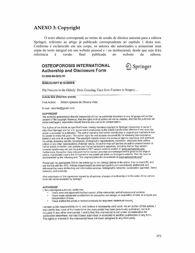
205
ANEXO 3: Copyright
O texto abaixo corresponde ao termo de sessão de direitos autorais para a editora Springer, referente ao artigo já publicado correspondente ao capítulo 1 desta tese. Conforme é esclarecido em seu corpo, os autores são autorizados a armazenar uma cópia do texto integral em seu website pessoal e / ou institucional, desde que seja feita referência à versão final publicada no website da editora.
206
Edison Iglesias de Oliveira Vidal
207
Declaração
As cópias de artigos de minha autoria ou de minha co-autoria, já publicados ou submetidos para publicação em revistas científicas ou anais de congressos sujeitos a arbitragem, que constam da minha Tese de Doutorado, intitulada “Aspectos epidemiológicos das fraturas do fêmur proximal em idosos”, não infringem os dispositivos da Lei no 9,610/98, nem o direito autoral de qualquer editora.
Campinas, 10 de junho de 2010.
__________________________ ___________________________________ Edison Iglesias de Oliveira Vidal Prof. Dr. Djalma de Carvalho Moreira Filho