m´etodo de galerkin descontínuo para dois problemas de convecc ...

UNIVERSIDADE FEDERAL DO PARANASHUQIN WANG

METODO DE GALERKIN DESCONTINUOPARA DOIS PROBLEMAS DE

CONVECCAO-DIFUSAO

Curitiba, Setembro de 2015.

UNIVERSIDADE FEDERAL DO PARANASHUQIN WANG

METODO DE GALERKIN DESCONTINUOPARA DOIS PROBLEMAS DE

CONVECCAO-DIFUSAO

Tese de Doutorado apresentada ao Programade Pos-Graduacao em Matematica Aplicada daUniversidade Federal do Parana, como requisitoparcial a obtencao do Tıtulo de Doutor emMatematica.

Orientador: Prof. Dr. Jinyun Yuan.Co-orientador: Prof. Dr. Yujiang Wu.

Curitiba, Setembro de 2015.

W246M Wang, Shuqin Método de Galerkin descontínuo para dois problemas de convecção-difusão/ Shuqin Wang. – Curitiba, 2015. 86 f. : il. color. ; 30 cm.

Tese - Universidade Federal do Paraná, Setor de Ciências Exatas, Programa de Pós-graduação em Matemática Aplicada, 2015.

Orientador: Junyun Yuan – Co-orientador: Yujiang Wu. Bibliografia: p. 82-86.

1. Equações diferenciais não lineares - Soluções numericas. 2. Dinamica dos fluidos. 3. Matemática aplicada. I. Universidade Federal do Paraná. II.Yuan, Junyun. III. Wu, Yujiang . IV. Título.

CDD: 515.355

Aos meus pais e meu irmao.

i

Acknowledgements

Immeasurable appreciation and deepest gratitude for the help and support from the

following persons .

I am extremely thankful to my supervisor Prof. Jinyun Yuan, and co-supervisor

Prof. Yujiang Wu for their support, advices, guidance, valuable comments, sugges-

tions, and care, shelter in doing these researches.

I greatly appreciate Prof. Weihua Deng, who responded promptly and enthusias-

tically to my requests for comments despite his congested schedules.

I thank for all the help from the professors in UFPR, Prof. Saulo, Prof. Geovani,

Prof. Elizabeth, Prof. Matioli and other professors who I know.

I am also thankful to my friends in Brazil, Oscar, Kally, Aura, Elvis, Marcos, Diego,

Priscila, Leonardo and all the classmates from the Pos.

Above all, thanks to my parents and my brother for their support, understanding

and love.

ii

Resumo

Nesta tese consideramos dois tipos de problemas de conveccao-difusao, a saber, as

equacoes de Navier-Stokes para meios incompressıveis e dependentes do tempo e as

equacoes de conveccao-difusao espaco-fracionaria em duas dimensoes.

Para as equacoes de Navier-Stokes usamos o metodo das caracterısticas para lin-

earizar equacoes nao-lineares e introduzimos uma variavel auxiliar para reduzir a equacao

de ordem alta a um sistema de primeira ordem. Escolhendo-se cuidadosamente os fluxos

numericos e adicionando os termos de penalizacao propomos um metodo de Galerkin

descontınuo caracterıstico local (CLDG) simetrico e estavel. Com essa simetria, e facil

provar estabilidade numerica e estimativas de erros. Experimentos numericos sao re-

alizados para verificar os resultados teoricos. Para os problemas de conveccao-difusao

espaco-fracionaria ainda utilizamos o metodo das caracterısticas para tratar a derivada

no tempo e os termos convectivos conjuntamente. Para o termo fracionario introduz-

imos algumas variaveis auxiliares para decompor a derivada de Riemann-Liouville na

integral de Riemann-Liouville e na derivada de ordem inteira. Em seguida um metodo

de Galerkin descontınuo hibridizado (HDG) e proposto. Finalmente usamos os metodos

analıticos para realizar a analise de estabilidade e estimativas de convergencia do es-

quema HDG.

Pelo nosso conhecimento, este e o primeiro trabalho que combina o metodo de

Galerkin descontınuo caracterıstico as equacoes de Navier-Stokes e as equacoes con-

veccao-difusao espaco-fracionaria em 2D. Estes esquemas tambem podem ser aplicados

e estudados em outros problemas. Os resultados numericos sao consistentes com os re-

sultados teoricos.

Palavras-chave: metodo das caracterısticas; metodo de Galerkin descontınuo; equacoes

de Navier-Stokes; equacoes de conveccao-difusao espaco-fracionaria.

iii

Abstract

In this thesis, we consider two kinds of convection-diffusion problems, namely the clas-

sical time-dependent incompressible Navier-Stokes equations and the space-fractional

convection-diffusion equations in two dimensions.

For Navier-Stokes equations, we use the method of characteristics to make nonlinear

equations linear, and we introduce an auxiliary variable to reduce high-order equation

to one order system. Carefully choosing numerical fluxes and adding penalty terms,

a stable and symmetric characteristic local discontinuous Galerkin (CLDG) method is

proposed. With this symmetry, it is easy to perform numerical stability and error es-

timates. Numerical experiments are performed to verify theoretical results. For the

space-fractional convection-diffusion problems, we still use the method of characteris-

tics to tackle the time derivative and convective terms together. For the fractional

term, we introduce some auxiliary variables to split the Riemann-Liouville derivative

into Riemann-Liouville integral and integer order derivative. Thus a hybridized discon-

tinuous Galerkin method (HDG) is proposed. Finally we use general analytic methods

to perform the stability analysis and convergence estimates of the HDG scheme.

As far as we know, this is the first time the discontinuous Galerkin method and the

method of characteristics are combined to numerically solve the Navier-Stokes equations

and space-fractional convection-diffusion equations in 2D. These schemes can be applied

and further studied into other problems as well. The numerical results are consistent

with theoretical results.

Keywords: method of characteristics; discontinuous Galerkin method; Navier-Stokes

equations; space-fractional convection-diffusion equations.

iv

Contents

Resumo iii

Abstract iv

List of Figures vii

List of Tables ix

List of Symbols x

Introduction 1

1 Fundamental definitions and lemmas 6

1.1 Sobolev spaces and inequalities . . . . . . . . . . . . . . . . . . . . . . . . 6

1.2 Broken Sobolev spaces and fundamental lemmas . . . . . . . . . . . . . . 8

1.3 Fractional calculus . . . . . . . . . . . . . . . . . . . . . . . . . . . . . . . 12

1.3.1 Definitions and properties . . . . . . . . . . . . . . . . . . . . . . . 12

1.3.2 Fractional spaces and lemmas . . . . . . . . . . . . . . . . . . . . . 14

1.4 The method of characteristics . . . . . . . . . . . . . . . . . . . . . . . . . 16

1.4.1 The linear convective term . . . . . . . . . . . . . . . . . . . . . . 16

1.4.2 The nonlinear convective term . . . . . . . . . . . . . . . . . . . . 18

2 CLDG method for the incompressible Navier-Stokes equations 20

2.1 The incompressible Navier-Stokes equations . . . . . . . . . . . . . . . . . 20

2.2 Derivation of the numerical scheme . . . . . . . . . . . . . . . . . . . . . . 21

2.2.1 Mathematical setting of the Navier-Stokes equations . . . . . . . . 21

2.2.2 CLDG scheme . . . . . . . . . . . . . . . . . . . . . . . . . . . . . 22

2.2.3 Time discretization . . . . . . . . . . . . . . . . . . . . . . . . . . . 25

2.2.4 Existence and uniqueness of CLDG solution . . . . . . . . . . . . . 27

2.3 Stability analysis . . . . . . . . . . . . . . . . . . . . . . . . . . . . . . . . 28

v

2.4 Error analysis . . . . . . . . . . . . . . . . . . . . . . . . . . . . . . . . . . 30

2.4.1 Error in velocity . . . . . . . . . . . . . . . . . . . . . . . . . . . . 31

2.4.2 Error in pressure . . . . . . . . . . . . . . . . . . . . . . . . . . . . 36

2.5 Numerical experiments . . . . . . . . . . . . . . . . . . . . . . . . . . . . . 41

3 HDG method for fractional convection-diffusion equations 58

3.1 Fractional convection-diffusion problem . . . . . . . . . . . . . . . . . . . 58

3.2 Fractional norms in variational norms . . . . . . . . . . . . . . . . . . . . 58

3.3 Derivation of numerical scheme . . . . . . . . . . . . . . . . . . . . . . . . 60

3.3.1 Dealing with time . . . . . . . . . . . . . . . . . . . . . . . . . . . 62

3.4 Stability analysis and error analysis . . . . . . . . . . . . . . . . . . . . . . 65

3.4.1 Stability analysis . . . . . . . . . . . . . . . . . . . . . . . . . . . . 65

3.4.2 Error analysis . . . . . . . . . . . . . . . . . . . . . . . . . . . . . . 66

3.5 Numerical experiments . . . . . . . . . . . . . . . . . . . . . . . . . . . . . 74

4 Conclusions and perspectives 80

Bibliography 82

vi

List of Figures

1.1 Uniform triangular meshes. . . . . . . . . . . . . . . . . . . . . . . . . . . 9

1.2 Nonuniform triangular meshes. . . . . . . . . . . . . . . . . . . . . . . . . 9

2.1 Condition number of the corresponding matrix for the CLDG scheme for

(2.9) vs the reciprocal of spatial step h with ∆t = 10−3, Re = 106. . . . . 41







2.5 The contour of exact solution u1(t = 0.25) of Example 2.1, Re = 1012. . . 44

2.6 The contour of numerical solution u1h(t = 0.25) of Example 2.1, Re = 1012. 45

2.7 The contour of exact solution u2(t = 0.25) of Example 2.1, Re = 1012. . . 45


2.9 The contour of exact solution p(t = 0.25) of Example 2.1, Re = 1012. . . . 46

2.10 The contour of numerical solution ph(t = 0.25) of Example 2.1, Re = 1012. 46

2.11 Exact solution u1(t = 1) of Example 2.2, Re = 1015. . . . . . . . . . . . . 48

2.12 Numerical solution u1h(t = 1) of Example 2.2, Re = 1015. . . . . . . . . . 48

2.13 Exact solution u2(t = 1) of Example 2.2, Re = 1015. . . . . . . . . . . . . 48

2.14 Numerical solution u2h(t = 1) of Example 2.2, Re = 1015. . . . . . . . . . 49

2.15 Exact solution p(t = 1) of Example 2.2, Re = 1015. . . . . . . . . . . . . . 49

2.16 Numerical solution ph(t = 1) of Example 2.2, Re = 1015. . . . . . . . . . . 49

2.17 Error and rate of velocity in Example 2.3, Re = 10. . . . . . . . . . . . . . 51

2.18 Error and rate of pressure in Example 2.3, Re = 10. . . . . . . . . . . . . 51

2.19 Error and rate of velocity in Example 2.3, Re = 104. . . . . . . . . . . . . 52

2.20 Error and rate of pressure in Example 2.3, Re = 104. . . . . . . . . . . . . 52

2.21 Error and rate of velocity in Example 2.3, Re = 1016. . . . . . . . . . . . . 52

2.22 Error and rate of pressure in Example 2.3, Re = 1016. . . . . . . . . . . . 53

vii

2.23 Exact solution u1(t = 0.01) of Example 2.4, Re = 108. . . . . . . . . . . . 54

2.24 Numerical solution u1h(t = 0.01) of Example 2.4, Re = 108. . . . . . . . . 55

2.25 Exact solution u2(t = 0.01) of Example 2.4, Re = 108. . . . . . . . . . . . 55

2.26 Numerical solution u2h(t = 0.01) of Example 2.4, Re = 108. . . . . . . . . 55

2.27 Exact solution p(t = 0.01) of Example 2.4, Re = 108. . . . . . . . . . . . . 56

2.28 Numerical solution ph(t = 0.01) of Example 2.4, Re = 108. . . . . . . . . . 56



2.31 The contour of numerical solution ph(t = 0.05) of Example 2.4, Re = 10. . 57

3.1 All triangles in x-direction affected by Gauss point (denoted by black

square). . . . . . . . . . . . . . . . . . . . . . . . . . . . . . . . . . . . . . 74

3.2 All triangles in y-direction affected by Gauss point (denoted by black

square). . . . . . . . . . . . . . . . . . . . . . . . . . . . . . . . . . . . . . 74

3.3 Exact solution u(t = 0.05). . . . . . . . . . . . . . . . . . . . . . . . . . . 77

3.4 Numerical solution uh(t = 0.05), h = 14 . . . . . . . . . . . . . . . . . . . . . 77


3.6 Numerical solution uh(t = 0.05), h = 116 . . . . . . . . . . . . . . . . . . . . 78

3.7 Exact solution u(t = 0.1). . . . . . . . . . . . . . . . . . . . . . . . . . . . 78




viii

List of Tables

2.1 The L2−norm errors and convergence rates of velocity and pressure for

Example 2.1 with T = 0.25, Re = 103. . . . . . . . . . . . . . . . . . . . . 43


Example 2.1 with T = 0.25, Re = 106. . . . . . . . . . . . . . . . . . . . . 44


Example 2.1 with T = 0.25, Re = 1012. . . . . . . . . . . . . . . . . . . . 44


Example 2.2 with T = 0.5, Re = 102. . . . . . . . . . . . . . . . . . . . . . 47


Example 2.2 with T = 0.5, Re = 108. . . . . . . . . . . . . . . . . . . . . . 47


Example 2.2 with T = 0.5, Re = 1015. . . . . . . . . . . . . . . . . . . . . 47


Example 2.3 with T = 0.5, Re = 102. . . . . . . . . . . . . . . . . . . . . . 50


Example 2.3 with T = 0.5, Re = 108. . . . . . . . . . . . . . . . . . . . . . 50


Example 2.3 with T = 0.5, Re = 1015. . . . . . . . . . . . . . . . . . . . . 51


Example 2.4 with T = 0.05, Re = 102. . . . . . . . . . . . . . . . . . . . . 54

2.11 The L2−norm errors of velocity and pressure for Example 2.4 with T =

0.05, Re = 108. . . . . . . . . . . . . . . . . . . . . . . . . . . . . . . . . . 54

3.1 Errors and convergence orders of Example 3.1 with c1 = Γ(5−α)Γ(6) , c2 = Γ(3−β)

Γ(2) . 75

3.2 Errors and convergence orders of Example 3.1 with c1 =Γ(2−α)Γ(6) , c2 =

Γ(2−β)Γ(6) . 76

ix

List of Symbols

DG discontinuous Galerkin method

LDG local discontinuous Galerkin method

CLDG characteristic local discontinuous Galerkin method

HDG hybridized discontinuous Galerkin method

Rd d-dimensional Euclidean space

Cd d-dimensional complex numbers space

‖ · ‖0 L2-norm

‖ · ‖1 H1-norm

‖ · ‖−1 the norm of space H−1

| · |1 H1-semi-norm

v vector function

v matrix function

∇u gradient operator for function u

∇ · u divergence operator for function u

∆u Laplace operator for function u

Pk the space of all polynomials of degree ≤ k

x

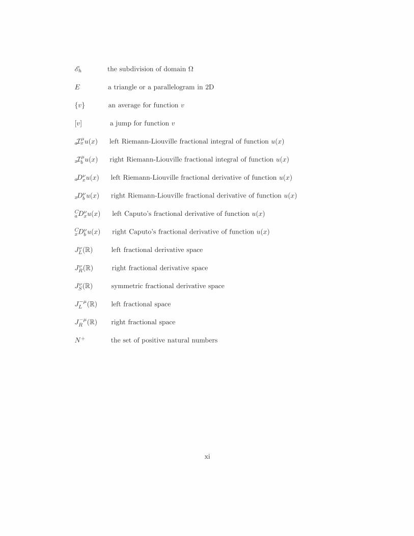
Eh the subdivision of domain Ω

E a triangle or a parallelogram in 2D

v an average for function v

[v] a jump for function v

aIµxu(x) left Riemann-Liouville fractional integral of function u(x)

xIµb u(x) right Riemann-Liouville fractional integral of function u(x)

aDνxu(x) left Riemann-Liouville fractional derivative of function u(x)

xDνb u(x) right Riemann-Liouville fractional derivative of function u(x)

CaD

νxu(x) left Caputo’s fractional derivative of function u(x)

CxD

νb u(x) right Caputo’s fractional derivative of function u(x)

JνL(R) left fractional derivative space

JνR(R) right fractional derivative space

JνS(R) symmetric fractional derivative space

J−µL (R) left fractional space

J−µR (R) right fractional space

N+ the set of positive natural numbers

xi

Introduction

In this thesis, we mainly consider two kinds of convection-diffusion problems: the clas-

sical time-dependent incompressible Navier-Stokes equations and the space-fractional

convection-diffusion equations.

Model one

In 1755, Swiss mathematician Leonhard Euler derived the Euler equations to describe

an ideal fluid without consider the effects of viscosity. In 1821, French engineer Claude-

Louis Navier introduced the element of viscosity for the more realistic and more difficult

problem of viscous fluids. Because of the physical significance of the viscosity coefficient,

Claude-Louis Marie Henri Navier’s name is associated with the famous Navier-Stokes

equations. Untill 1845 Irish mathematician-physicist George Gabrid Stokes published

a derivation of the equations in a manner that is currently understood. Then, George

Gabrid Stokes’s name was attached with the Navier-Stokes equations.

Navier-Stokes equations are useful because they describe many scientific and engi-

neering phenomena. They are used to model weather, ocean currents, water flow in a

pipe and air flow around a wing. Navier-Stokes equations are still used to help with

the design of aircrafts and cars, the study of blood flow, the design of power stations,

the analysis of pollution [4, 6, 17, 18, 30, 37, 44, 46, 56]. The reciprocal of fluid vis-

cosity coefficient ν is called Reynolds number. For very low Reynolds numbers and

simple geometries, it is often possible and easy to find explicit formulas for solutions

to Navier-Stokes equations in a computation. For high Reynolds numbers, in turbulent

flow there begin to be eddies with a wide range of sizes. To capture all these eddies

in a computation, one needs a large amount of information, for example, memory and

datum. Such flows can be described in many situations, for example, blood flow in large

caliber vessels, fluid-structure interaction, aerodynamics, geophysical and astrophysical

flow modeling. Despite of half a century of vigorous efforts, there is still a lack of sys-

tematic understanding how different scales interact to form the inertial range from a

smooth initial condition. Therefore, the description of the behavior of the solutions of

the Navier-Stokes equations at high Reynolds numbers is the heart of the problem. The

choice of the singularity problem for the incompressible Navier-Stokes equations as one

of the million prize problems highlight the fundamental role that mathematical analysis

may play in this topic.

In Chapter 2, we shall design a new scheme to recast the time-dependent incom-

pressible Navier-Stokes equations. Our scheme is based on standard local discontinuous

Galerkin method and the method of characteristics. In this work, we devote to recover

the solutions with high Reynolds numbers. For the sake of simplicity, we just consider

the full Navier-Stokes equations with Dirichlet boundary conditions: these equations can

be written by

∂tu+ (u · ∇)u− ν∆u+∇p = f , (x, t) ∈ Ω× J,

∇ · u = 0, (x, t) ∈ Ω× J,

u(x, t) = 0, (x, t) ∈ ∂Ω× J,

u(x, 0) = u0(x), x ∈ Ω,

(1)

where Ω is a bounded polygonal domain in R2 with Lipschitz continuous boundary ∂Ω

and J = [0, T ], 0 < T <∞.

Because of the inherent performances of the Navier-Stokes or Stokes equations in

characterizing the turbulence in fluids or gases, from finite element method to discontin-

uous Galerkin method a lot of researches on these topics have been done [4, 15, 17, 18, 29,

31, 32, 37, 51]. As our knowledge, there are few works on discontinuous Galerkin method

for solving the time-dependent incompressible Navier-Stokes equations, and much less

on local discontinuous Galerkin method (LDG), which motivates us to consider LDG

method for the full Navier-Stokes equations. Splitting the nonlinearity and incompress-

ibility, and using discontinuous or continuous Galerkin method in space, Girault et al

[29] solved the time-dependent incompressible Navier-Stokes equations using penalty

discontinuous Galerkin method [50]. Comparing with the work [29], we use different DG

method to discretize spatial space and get better numerical results (see Chapter 2).

In Chapter 2 of this thesis, we use the local discontinuous Galerkin method to dis-

cretize the spatial space of the considered equation. It seems that the following ad-

vantages can be obtained: 1) by introducing local auxiliary variable, the order of the

diffusion term can be reduced. Arising from using penalty terms the symmetric formu-

lation makes stability and error analysis possible; 2) the introduced auxiliary variable

2

σ =√ν∇u lessens challenges caused by big Reynolds numbers since

√ν is not as small

as ν when ν is small enough. The lucky thing is that we still keep the general advantages

of discontinuous Galerkin method, i.e., the high order accuracy, the hp-adaptivity, and

the high parallelizability, etc..

Here we use the method of characteristics [6, 27] to tackle time derivative term and

nonlinear convective term together for the considered equation with first order accuracy

in time. The method of characteristics has many advantages compared to a high order

Runger-Kutta scheme or a high order finite difference scheme, such as 1) efficient in

solving the advection-dominated diffusion problems; 2) easily obtaining the existence

and uniqueness of the solutions of the discretized system; 3) making nonlinear equations

linear and conveniently tackling nonlinear obstacles; 4) easily performing numerical sta-

bility analysis.

In summary, the work described in Chapter 2 is an extension of local discontinuous

Galerkin methods for the Stokes system [15] with the characteristic local discontinuous

Galerkin scheme to the time-dependent incompressible Navier-Stokes equations.

Model two

In Chapter 3, we shall consider the time-dependent space-fractional convection-diffusion

problem for u in the form:

∂tu+ b · ∇u− c1∂αu∂xα − c2

∂βu∂yβ

= f, (x, t) ∈ Ω× J,

u(x, t) = 0, (x, t) ∈ ∂Ω× J,

u(x, 0) = u0(x), x ∈ Ω,

(2)

where Ω ∈ R2 is rectangular domain with Lipschitz continuous boundary ∂Ω, and J =

[0, T ], 0 < T < ∞, the superdiffusion operators ∂α

∂xα and ∂β

∂yβwill be defined in Chapter

3.

Let us briefly review the development of numerical methods for fractional convection-

diffusion equations. Several authors have proposed a variety of higher-order finite dif-

ference schemes for solving time-fractional convection-diffusion equations, for example

[23, 36, 58, 60], and solving space-fractional convection-diffusion equations [10, 38]. In

[40] and [42], W. Mclean and K. Mustapha have used piecewise-constant and piecewise-

linear discontinuous Galerkin (DG) methods to solve time-fractional diffusion and wave

equations, respectively. However, these methods require more computational costs (see

[41]). In order to tackle those problems, in [41] W. Mclean has proposed an efficient

3

scheme called fast summation by interval clustering to reduce the implementation mem-

ory. Furthermore, in [26] Deng and Hesthaven have developed discontinuous Galerkin

method for fractional spatial derivatives and given a fundamental frame to combine the

discontinuous Galerkin method with fractional operators in one dimension. In [59] Xu

and Hesthaven have applied the DG method to fractional convection-diffusion equations

in one dimension. In two dimensional case, Ji and Tang [34] have applied the DG method

to recast fractional diffusion equations in rectangular meshes with the optimal conver-

gence order O(hk+1) numerically. However, there were no theoretical results. So far very

few works have considered fractional problems in triangular meshes. This motivates us

to consider a successful DG method for solving fractional problems in triangular meshes.

Fractional differential equations (FDEs) have become more and more popular in

applied science and engineering field recently. The history and mathematical background

of fractional differential operators are given in [45] with definitions and applications of

fractional calculus. This kind of equations has been used increasingly in many fields,

for example, in Nature [35] fractional operators applied in fractal stream chemistry and

its implications for contaminant transport in catchments, in [39] the fractional calculus

motivated in bioengineering, and its application as a model for physical phenomena

exhibiting anomalous diffusion, Levy motion, turbulence [5, 8, 53], etc.

In Chapter 3, we shall design a stable and accurate discontinuous Galerkin method

for the considered equation (2). The stability and error analysis are proved in multi-

ple dimensions. This development is built on the extension work on DG for previous

work found in [26, 59], where a qualitative study of the high order local discontinuous

Galerkin method was discussed and some theoretical results were offered in one space

dimension. In order to perform the error analysis, the authors defined some projection

operators to prove error results. Unfortunately, we can not extend the defined projection

operators into two dimensional case easily (see [26, 59]). Hence, to avoid this difficulty,

a different DG method is obtained in Chapter 3 by carefully choosing numerical fluxes

and adding penalty terms. The presented hybridized discontinuous Galerkin (HDG)

method has the following attractive properties: 1) The HDG method can be used for

other fractional problems, for example, fractional diffusion equations; 2) It has excellent

provable stability. One can prove the stability in any space dimension; 3) Theoretically,

the error estimates are proved more easily with general analytical methods in any space

dimension.

4

The outline of thesis

Let us give a more detailed description of the content of this thesis.

In Chapter 1, firstly, we review some basic definitions of Sobolev spaces and broken

Sobolev spaces, some useful lemmas for discontinuous Galerkin method. Then we de-

scribe some definitions of fractional calculus and some fractional variational norms and

spaces. Finally, we shall introduce the method of characteristics with different cases:

the linear case and nonlinear case.

In Chapter 2, by combining the method of characteristics and the local discontinu-

ous Galerkin method and carefully constructing numerical fluxes, we design a variational

formulation for the time-dependent incompressible Navier-Stokes equation in R2. The

nonlinear stability of the proposed symmetric variational formulation is proved. More-

over, for general triangulations we derive an a priori estimate for the L2-norm of the

errors in both velocity and the pressure. The proposed scheme works well for a wide

range of Reynolds numbers such as Re = 106, 108, 1012, 1015, 1016.

In Chapter 3, a hybridized discontinuous Galerkin method is proposed for solving

2D fractional convection-diffusion equations containing derivatives of fractional order in

space on a finite domain. The Caputo’s or Riemann-Liouville derivative is chosen as

the representation of spatial derivative. Combining the method of characteristics and

the hybridized discontinuous Galerkin method, the symmetric variational formulation is

constructed. The stability of the presented scheme is proved. An order of k + 1/2 is

established for some fractional convection-diffusion problems. Some numerical examples

are given to illustrate the numerical performance of our method. The first experiment

is performed to display the convergence order while the second experiment justifies the

benefits of this scheme. Both are tested with triangular meshes.

Finally, in Chapter 4 we conclude these works and give some future perspectives.

5

Chapter 1

Fundamental definitions and

lemmas

Discontinuous Galerkin method was introduced in 1973 by Reed and Hill [49], in the

framework of neutron transport (steady state linear hyperbolic equations). A major

development of the discontinuous Galerkin method was carried out by Cockburn and

collaborators. In a series of papers [15, 16, 19, 21, 22], they established a framework

to easily solve nonlinear time-dependent hyperbolic conservation laws, using explicit,

nonlinearly stable high-order Runge-Kutta time discretization [22] and discontinuous

Galerkin spatial discretization [17, 18].

In this chapter, we shall review some basic definitions and results for mathematical

setting of the discontinuous Galerkin (DG) method. Firstly, we describe some Sobolev

spaces. Afterwards, we introduce broken Sobolev space, the natural working spaces for

DG.

1.1 Sobolev spaces and inequalities

Throughout this section, let Ω denote a bounded polygonal domain in Rd, d ∈ N+. The

L2(Ω) and L∞(Ω) are the classical space of square integrable functions with the inner

product (f, g) =∫Ω fg dx and the space of bounded functions, respectively [14, 50].

L∞(Ω) =v :‖ v ‖L∞(Ω)<∞

, ‖ v ‖L∞(Ω)= ess sup

|v(x)| : x ∈ Ω

.

It is well known that C(Ω) and C∞0 (Ω) are the space of continuous functions and the

space of infinitely differentiable functions with compact support, respectively. Generally

6

the Sobolev space Hs(Ω) for integer s is denoted by

Hs(Ω) =v ∈ L2(Ω) : ∀ 0 ≤ |α| ≤ s,Dαv ∈ L2(Ω)

,

where Dαv = ∂|α|v∂x

α11 ···∂xαd

d

, |α| =∑di=1 αi. Similarly, the space H1(Ω) is defined by

H1(Ω) =v ∈ L2(Ω) : Dv ∈ L2(Ω)

.

H10 (Ω) denotes the closure of C

∞0 (Ω) in H1(Ω), and H−1(Ω) is the dual space of H1

0 (Ω).

Assume that k is nonnegative integer, Ck(Ω) =u : Ω 7→ R|Dαu ∈ C(Ω), |α| ≤ k

is the space of k times continuously differentiable functions equipped with the norm

‖ u ‖Ck(Ω)=∑

|α|≤ksupx∈Ω

|Dαu(x)|,

where Ω is the closure of Ω.

Let 0 < β ≤ 1, Ck,β(Ω) =u ∈ Ck(Ω)| supx 6=y,x,y∈Ω |Dαu(x)−Dαu(y)|

|x−y|β < +∞, |α| = k

is the space of k + β times Holder continuous functions equipped with the norm

‖ u ‖Ck,β(Ω)=‖ u ‖Ck(Ω) + supx 6=y,x,y∈Ω

|Dαu(x)−Dαu(y)||x− y|β .

For any Banach space X let Lp[0, T ;X], 1 ≤ p < ∞, and L∞[0, T ;X] denote the

spaces of p−integrable functions with norms

‖ v ‖Lp[0,T ;X]=(∫ T

0‖ v(t) ‖pX

)1/p, ‖ v ‖L∞[0,T ;X]= esssupt∈[0,T ] ‖ v ‖X<∞.

Let H1[0, T ;X] denote the space of functions with square integral derivatives with norm

‖ v ‖H1[0,T ;X]=(∫ T

0‖ v ‖2X dt+

∫ T

0‖ ∂tv ‖2X dt

)1/2.

Here, we introduce some inequalities [14, 50] that are used many times in our analysis.

• Holder’s inequality:

∫

Ω

∣∣f(x)g(x)∣∣dx ≤

(∫

Ω

∣∣f(x)∣∣pdx

) 1p(∫

Ω

∣∣g(x)∣∣qdx

) 1q,

where 1p +

1q = 1 with 1 ≤ p, q < ∞ and f ∈ Lp(Ω), g ∈ Lq(Ω). If p = q = 2, this

inequality becomes Cauchy-Schwarz’s inequality.

7

Similarly, Holder’s inequality for sums states that

n∑

k=1

∣∣akbk∣∣ ≤

( n∑

k=1

|ak|p)1/p( n∑

k=1

|bk|q)1/q

,

where (a1, · · · , an), (b1, · · · , bn) ∈ Rn or Cn.

• Young’s inequality:

∀ǫ > 0, ∀a, b ∈ R, ab ≤ ǫ

2a2 +

1

2ǫb2.

Lemma 1.1. (Poincare-Friedrichs inequality) [50] The classical Poincare-Friedrichs in-

equality in H1(Ω) says that there is a constant C such that

∀ v ∈ H1(Ω), ‖ v ‖0≤ C(‖∇v‖0 +

∣∣∫

∂Ωv∣∣). (1.1)

Consequently, we have

∀ v ∈ H10 (Ω), ‖ v ‖0≤ C‖∇v‖0. (1.2)

See Chapter 3 of [50].

1.2 Broken Sobolev spaces and fundamental lemmas

As we know, discontinuous Galerkin method is a type of finite element method. They

share many properties and results, however discontinuous Galerkin method uses com-

pletely discontinuous piecewise polynomial spaces for numerical solutions and test func-

tions. Comparing with classical finite element method, discontinuous Galerkin method

have the following attractive properties:

• It can be easily designed for any order of accuracy. In fact, the order of accuracy

can be locally determined in each simplex.

• It can handle complicated geometries, i.e, it can be used on arbitrary triangula-

tions, even those with hanging nodes.

• It has high parallelizability.

• It has excellent provable nonlinear stability.

8

−1 −0.5 0 0.5 1−1

−0.8

−0.6

−0.4

−0.2

0

0.2

0.4

0.6

0.8

1uniform mesh

x

y

Fig. 1.1: Uniform triangular meshes.

−1 −0.5 0 0.5 1−1

−0.8

−0.6

−0.4

−0.2

0

0.2

0.4

0.6

0.8

1nonuniform mesh

x

y

Fig. 1.2: Nonuniform triangular meshes.

The broken Sobolev spaces [50] are natural spaces to work with discontinuos Galerkin

method. These spaces depend strongly on the partition of the domain. Let Ω be a

polygonal domain subdivided into elements E (see Figures 1.1-1.2). Here E is a triangle

or a quadrilateral in 2D. We assume that the intersection of two elements is either empty,

or an edge (2D). The mesh is called a regular mesh if

∀E ∈ Eh,hEρE

≤ C,

where Eh is the subdivision of Ω, C is a constant, hE is the diameter of the element E,

i.e., hE = supx,y∈E ‖ x − y ‖ and ρE is the diameter of the inscribed circle in element

E. Throughout this thesis h = maxE∈EhhE .

We introduce the broken Sobolev space for any real number s,

Hs(Eh) =v ∈ L2(Ω) : ∀E ∈ Eh, v|E ∈ Hs(E)

,

equipped with the broken Sobolev norm:

‖ v ‖Hs(Eh)=( ∑

E∈Eh

‖ v ‖2Hs(E)

)1/2.

Jumps and averages: We denote by E Bh the set of edges of the subdivision Eh.

Let E ih denote the set of interior edges, E b

h = E Bh \E i

h the set of edges on ∂Ω. With each

edge e, we have a unit normal vector ne. If e is on the boundary ∂Ω, then ne is taken

to be the unit outward vector normal to ∂Ω [50].

9

If v belongs to H1(Eh), the trace of v along any side of one element E is well defined.

If two elements Ee1 and Ee2 are neighbors and share one common side e, there are two

traces of v belonging to e. We assume that the normal vector ne is oriented from Ee1 to

Ee2, and an average and a jump for v can be defined by

v =1

2(v|∂Ee

1+ v|∂Ee

2), [v] = (v|∂Ee

1− v|∂Ee

2), ∀e ∈ ∂Ee1

⋂∂Ee2 .

If e is on ∂Ω, we have

v = [v] = v|∂E , ∀e ∈ ∂E⋂∂Ω.

Next, we shall recall some inequalities, which are important tools for theoretical

analysis.

Lemma 1.2. (Continuous Gronwall inequality) [50] Assume that f, g, h are piecewise

continuous non-negative functions defined on (a, b), and g is nondecreasing. If there

exists a positive constant C independent of t such that

∀ t ∈ (a, b), f(t) + h(t) ≤ g(t) + C

∫ t

af(s)ds,

then

∀ t ∈ (a, b), f(t) + h(t) ≤ eC(t−a)g(t).


Lemma 1.3. (Discrete Gronwall inequality) [50] Let ∆t, B,C > 0 and (an), (bn), (cn)

be sequences of non-negative numbers satisfying

∀ n ≥ 0, an +∆tn∑

i=0

bi ≤ B + C∆tn∑

i=0

ai +∆tn∑

i=0

ci,

then, if C∆t < 1,

∀ n ≥ 0, an +∆t

n∑

i=0

bi ≤ eC(n+1)∆t(B +∆t

n∑

i=0

ci).


Theorem 1.4. (Approximation property) [50] Assume that E is a triangle or parallelo-

10

gram in 2D or a tetrahedron or hexahedron in 3D. Let v ∈ Hs+1(E) for s ≥ 0 and k ≥ 0.

Then, there exists a constant C independent of v and hE and a function v ∈ Pk(E), such

that

∀ 0 ≤ q ≤ s, ‖ v − v ‖Hq(E)≤ Chmin(k,s)+1−qE

∣∣v∣∣Hs(E)

, (1.3)

where Pk(E) is the space of polynomials of degree less than or equal to k.


Trace inequalities: [50] Let E be a element with a diameter hE . Then, ∀ e ⊂ ∂E

for any function v ∈ Hs(E), there exists a constant C independent of hE and v such

that

s ≥ 1, ‖ v ‖L2(e)≤ C|e|1/2|E|−1/2(‖ v ‖L2(E) +hE ‖ ∇v ‖L2(E)

),

s ≥ 2, ‖ ∇v · ne ‖L2(e)≤ C|e|1/2|E|−1/2(‖ ∇v ‖L2(E) +hE ‖ ∇2v ‖L2(E)

).

(1.4)


Lemma 1.5. (Inverse inequality) [50] There exists a constant C independent of hE such

that for any polynomial function v of degree k defined on E, we have

∀ 0 ≤ j ≤ k, ‖ ∇jv ‖L2(E)≤ Ch−jE ‖ v ‖L2(E) . (1.5)


Next, we shall review two lemmas for our analysis. The first one is the standard

approximation result for any linear continuous projection operator Π from Hs+1(E)

onto Vh(E) =v; v∣∣E∈ Pk(E)

satisfying Πv = v for any v ∈ Pk(E). The second one is

the standard trace inequality.

Lemma 1.6. [9] Let v ∈ Hs+1(E), s ≥ 0 and Π be a linear continuous projection

operator from Hs+1(E) onto Vh(E) such that Πv = v for any v ∈ Pk(E). Then, for

m = 0, 1, we have

∣∣v −Πv∣∣Hm(E)

≤ Chmin(s,k)+1−mE ‖ v ‖Hs+1(E),

‖ v −Πv ‖L2(∂E)≤ Chmin(s,k)+ 1

2E ‖ v ‖Hs+1(E) .

(1.6)

11

Lemma 1.7. [9] There exists a generic constant C which is independent of hE such that

for any v ∈ Vh(E) we have

‖ v ‖L2(∂E)≤ Ch− 1

2E ‖ v ‖L2(E) . (1.7)

1.3 Fractional calculus

1.3.1 Definitions and properties

This section is devoted to definitions and properties in fractional calculus. The theory of

derivatives of non-integer order goes back to the Leibniz’s note in his list to L’Hospital

[45]. About three centuries, the theory of fractional derivatives developed mainly in a

pure theoretical field of mathematics. Until last few decades the integrals of non-integer

order were pointed out by many researchers. Those integrals are used for the description

of some properties of various real materials and many phenomena in physics, engineering,

chemistry [39, 45, 47, 52, 53], etc.

In Chapter 3, we will consider a hybridized discontinuous Galerkin (HDG) method for

solving 2D space-fractional convection-diffusion problems. Before giving the numerical

method for those fractional equations, we have to review several definitions and lemmas

for calculus. In the following we recall some definitions of fractional integrals, derivatives,

and their properties.

Definition 1.1. [28, 47, 59] For any µ > 0, the left (right) Riemann-Liouville fractional

integral of function u(x) defined on (a, b) is denoted by

(1) Left Riemann-Liouville fractional integral:

aIµxu(x) =∫ x

a

(x− ξ)µ−1

Γ(µ)u(ξ)dξ,

(2) Right Riemann-Liouville fractional integral:

xIµb u(x) =∫ b

x

(ξ − x)µ−1

Γ(µ)u(ξ)dξ,

where Γ(µ) =∫∞0 e−ttµ−1dt, which is Euler’s gamma function.

Definition 1.2. [28, 47, 59] For any ν > 0, n − 1 < ν < n, n ∈ N+, the left (right)

Riemann-Liouville fractional derivative of function u defined on (a, b) is denoted by

12

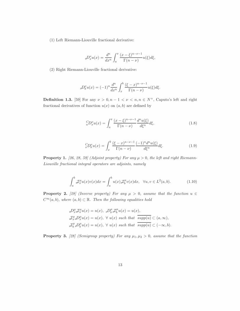
(1) Left Riemann-Liouville fractional derivative:

aDνxu(x) =

dn

dxn

∫ x

a

(x− ξ)n−ν−1

Γ(n− ν)u(ξ)dξ,

(2) Right Riemann-Liouville fractional derivative:

xDνb u(x) = (−1)n

dn

dxn

∫ b

x

(ξ − x)n−ν−1

Γ(n− ν)u(ξ)dξ.

Definition 1.3. [59] For any ν > 0, n − 1 < ν < n, n ∈ N+, Caputo’s left and right

fractional derivatives of function u(x) on (a, b) are defined by

CaD

νxu(x) =

∫ x

a

(x− ξ)n−ν−1

Γ(n− ν)

dnu(ξ)

dξndξ, (1.8)

CxD

νb u(x) =

∫ b

x

(ξ − x)n−ν−1

Γ(n− ν)

(−1)ndnu(ξ)

dξndξ. (1.9)

Property 1. [26, 28, 59] (Adjoint property) For any µ > 0, the left and right Riemann-

Liouville fractional integral operators are adjoints, namely

∫ b

aaIµxu(x)v(x)dx =

∫ b

au(x)xIµb v(x)dx, ∀u, v ∈ L2(a, b). (1.10)

Property 2. [28] (Inverse property) For any µ > 0, assume that the function u ∈C∞(a, b), where (a, b) ⊂ R. Then the following equalities hold

aDµxaIµxu(x) = u(x), xD

µb xI

µb u(x) = u(x),

aIµx aDµxu(x) = u(x), ∀ u(x) such that supp(u) ⊂ (a,∞),

xIµb xDµb u(x) = u(x), ∀ u(x) such that supp(u) ⊂ (−∞, b).

Property 3. [28] (Semigroup property) For any µ1, µ2 > 0, assume that the function

13

u ∈ Lp(a, b), p ≥ 1, where (a, b) ⊂ R. Then the following equalities hold

aIµ1x aIµ2x u(x) = aIµ1+µ2x u(x), ∀ x ∈ (a, b),

xIµ1b xIµ2b u(x) = xIµ1+µ2b u(x), ∀ x ∈ (a, b).

Property 4. [28] (Fourier transform property) For any µ > 0, assume that the function

u ∈ Lp(R), p ≥ 1. Then the Fourier transform of the left and right Riemann-Liouville

fractional integrals satisfy the following equations

F(−∞Iµxu(x)) = (iω)−µu(ω),

F(xIµ∞u(x)) = (−iω)−µu(ω),

where u(ω) denotes the Fourier transform of u, i.e.

u(ω) =

∫

Re−iωxu(x)dx.

Property 5. [28] (Fourier transform property) For any ν > 0, assume that the function

u ∈ C∞0 (Ω),Ω ⊂ R. Then the Fourier transform of the left and right Riemann-Liouville

fractional derivatives satisfy the following

F(−∞Dνxu(x)) = (iω)ν u(ω),

F(xDν∞u(x)) = (−iω)ν u(ω).

1.3.2 Fractional spaces and lemmas

In this subsection, we will recall some fractional derivative spaces setting for variational

solutions. In order to define associated fractional derivative spaces, we assume that

u ∈ C∞0 (a, b), (a, b) ⊂ R. We extend u by zero outside of the interval (a, b).

Definition 1.4. [28] (Fractional derivative spaces) For any ν > 0, define the norms

(1) Left fractional derivative space:

‖ u ‖JνL(R):=

(‖−∞Dν

xu(x) ‖2L2(R) + ‖ u ‖2L2(R)) 1

2 ,

where

|u|JνL(R) :=‖−∞Dν

xu(x) ‖L2(R) .

14

(2) Right fractional derivative space:

‖ u ‖JνR(R):=

(‖ xD

ν∞u(x) ‖2L2(R) + ‖ u ‖2L2(R)

) 12 ,

where

|u|JνR(R) :=‖ xD

ν∞u(x) ‖L2(R) .

Let JνL(R) and JνR(R) be the closures of C∞0 (R) with respect to the norms ‖ · ‖Jν

L(R)

and ‖ · ‖JνR(R), respectively.

Next we review a norm whose definition is associated with the Fourier transform.

Definition 1.5. [28] For any ν > 0, define the norm

‖ u ‖Hν(R):=(|u|2Hν (R)+ ‖ u ‖2L2(R)

) 12 ,

where

|u|Hν(R) :=‖ |ω|ν u ‖L2(R) .

In the analysis of finite element method or discontinuous Galerkin method, we gen-

erally make use of the formula (−∞Dνxu,xD

ν∞u)L2(R). For this case, we need the following

theorem which is important for combing the fractional spaces and variational spaces.

Theorem 1.8. [28] For any ν > 0, n − 1 < ν < n, n ∈ N+, assume that u is a real

valued function, then

(−∞D

νxu,xD

ν∞u)L2(R) = cos(νπ) ‖−∞Dν

xu ‖2L2(R) . (1.11)

Remark 1.1. Note that cos(νπ) > 0 when ν ∈ (−12 + 2mπ, 12 + 2mπ),m ∈ N . In this

case, we can define a norm which is available.

Definition 1.6. [28] (Symmetric fractional derivative space) For any ν > 0, ν 6= m −1/2,m ∈ N . Define the norm

‖ u ‖JνS(R):=

(∣∣ cos(νπ) ‖ Dνu ‖2L2(R)∣∣2+ ‖ u ‖2L2(R)

) 12 ,

and

|u|JνS(R) :=

∣∣ cos(νπ) ‖ Dνu ‖2L2(R)∣∣ 12 ,

15

where JνS(R) is the closure of C∞0 (R) with respect to ‖ · ‖Jν

S(R).

Let Ω = (a, b) be a bounded open subinterval of R. We now restrict the fractional

derivative spaces to Ω.

Definition 1.7. [28] Define the spaces JνL,0(Ω), JνR,0(Ω),H

ν0 (Ω), J

νS,0(Ω) as the closures

of C∞0 (Ω) under their respective norms.

Theorem 1.9. [28] (Fractional Poincare-Friedrichs) For u ∈ Hν0 (Ω), we have

‖ u ‖L2(Ω)≤ C|u|Hν0 (Ω), (1.12)

and for 0 < s < ν, s 6= n− 1/2, n ∈ N

|u|Hs0 (Ω) ≤ C|u|Hν

0 (Ω). (1.13)

See the proof in [28].

1.4 The method of characteristics

The idea of the method of characteristics dates back to the work of Douglas and Russell

[27] in 1982. Later on Arbogast [2, 3] extended the method of characteristics to transport

problems. Recently Chen combined the method of characteristics with mixed discon-

tinuous Galerkin method and finite element method for advection-dominated diffusion

and degenerate parabolic problems, respectively [11, 12]. In many convection-diffusion

problems arising in physical phenomena, convection essentially dominates diffusion. In

general, we shall consider the method of characteristics to treat some convection-diffusion

problems to reflect the hyperbolic nature of models. The convection-diffusion problems

mainly contain two cases: One is the problem with linear convective term, another one

is the problem with nonlinear convective term. Next we shall introduce the method of

characteristics with those two cases.

1.4.1 The linear convective term

We shall consider applying the method of characteristics to the time-dependent advection

diffusion problem for u on the bounded domain Ω ⊂ Rd, d = 1, 2, 3, with Lipschtiz

16

boundary ∂Ω [2, 24, 27]:

φ∂tu+ b · ∇u−∇ · (a∇u) = f, (x, t) ∈ Ω× J,

u(x, t) = gD, (x, t) ∈ ∂Ω× J,

u(x, 0) = u0(x), x ∈ Ω,

(1.14)

where J = [0, T ], 0 < T < ∞, φ(x) is a function bounded below and above by posi-

tive constants, b(x, t) is a bounded vector, a(x, t) is a positive semi-definite, bounded,

symmetric tensor, f ∈ L2(J ; Ω), gD ∈ L2(J ;H1/2(∂Ω)), u0 ∈ L2(Ω).

For each positive integer N , let 0 = t0 < t1 < · · · < tN = T be a partition of J into

subintervals Jn = (tn−1, tn], ∆t = tn − tn−1, 1 ≤ n ≤ N , and un = u(x, tn). The time

interval of interest is Jn, then the characteristic trace-back of the point x ∈ Ω is denoted

by x(x, t), and it satisfies the (time backward) ordinary differential equation

dxdt = b(x, t)/φ(x), tn−1 ≤ t < tn,

x(x, tn) = x.

(1.15)

From equality (1.15) we imply that

x− x(x, tn−1) =

∫ tn

tn−1

b(x(x, t), t)

φ(x(x, t))dt

≈ ∆tb(x(x, tn), tn)

φ(x(x, tn))

= ∆tb(x, tn)

φ(x).

Let ψ(x, t) =(φ2 + |b|2

)1/2, |b|2 = b21 + · · · + b2d. Then the characteristic direction

associated with the hyperbolic operator φ∂tu+ b · ∇u can be denoted by τ(x, t), where

∂τ =φ(x)

ψ(x, t)∂t +

b(x, t)

ψ(x, t)· ∇. (1.16)

Then the approximation of the directional derivative ∂u(x,t)∂τ(x,t) at time t = tn can be

∂u(x, tn)

∂τ(x, tn)≈ u(x, tn)− u(x(x, tn−1), tn−1)(|x− x(x, tn−1)|2 +∆t2

)1/2 .

17

Note that

φ∂tun + bn · ∇un = ψn

∂u(x, tn)

∂τ(x, tn)

≈ φu(x, tn)− u(x(x, tn−1), tn−1)

∆t.

(1.17)

For the method of characteristics, we need the assumption

φ ∈W 1,∞(Ω),b

φ∈ L∞(J ;W 1,∞(Ω)2),

0 < cl ≤ φ(x) ≤ cr <∞,∣∣∣b(x, t)φ(x)

∣∣∣+∣∣∣∇ ·

(b(x, t)φ(x)

)∣∣∣ ≤ C, (x, t) ∈ Ω× J,

(1.18)

where cl, cr, C are some constants. See the details in [2, 3, 24, 27].

In Chapter 3 we will use the above method of characteristics to solve space-fractional

convection-diffusion equations in 2D. In this case, b satisfies the assumption (1.18) and

φ = 1.

1.4.2 The nonlinear convective term

In this subsection, we focus on applying the method of characteristics to solve some

convection diffusion problems with nonlinear convective term. For the sake of simplicity,

we consider combining the method of characteristics to the Navier-Stokes equation, i.e.

∂tu+ (u · ∇)u− ν∆u+∇p = f , (x, t) ∈ Ω× J,

∇ · u = 0 (x, t) ∈ Ω× J,

u|∂Ω = gD(x, t), (x, t) ∈ ∂Ω× J,

u(x, 0) = u0(x), x ∈ Ω,

(1.19)

where Ω denotes a bounded open subset of Rd, d = 2, 3 with Lipschitz continuous bound-

ary ∂Ω, u(x, t) is the velocity of the fluid, p(x, t) is the kinematic pressure, ν is the

kinematic viscosity and f(x, t) is the body force.

Given a fluid flow with the velocity field u(x, t), the trajectory is a solution of the

18

following suitable differential equation

dx(x,s;t)dt = u(x(x, s; t), t),

x(x, s; s) = x,

(1.20)

where x(x, s; t) is the position at time of particle of fluid which is at point x at time

t = s, and x : (x, s; t) ∈ Ω× J × J 7→ x(x, s; t).

Lemma 1.10. [55] Assume that u ∈ C(C0,1(Ω)d) ∩ C(V ) (V = v ∈ H10 (Ω)

d|∇ ·v = 0 in Ω). If |s − t| is sufficiently small, then x 7→ x(x, s; t) is a quasi-isometric

homomorphism of Ω onto itself and its Jacobian equals to 1 a.e. on Ω.

Proof. See the proof in [55].

Define ψ(x, t) =(1 + |u|2

)1/2, then the material derivative of u can be rewritten as

a derivative in the direction τ(x, t)

∂tu+ (u · ∇)u = ψ∂u

∂τ. (1.21)

For each positive integer N , let 0 = t0 < t1 < · · · < tN = T be a partition of J

into subintervals Jn = (tn−1, tn], ∆t = tn − tn−1, 1 ≤ n ≤ N , and un = u(x, tn). For

x ∈ Ω, s = tn, with some deduction we have

x− x(x, tn; tn−1) =

∫ tn

tn−1

u(x(x, tn; t), t)dt ≈ ∆tu(x, tn).

Then, the backward difference approximation for direction τ(x, tn) is that

∂u(x, tn)

∂τ(x, tn)≈ u(x, tn)− u(x(x, tn; tn−1), tn−1)(|x− x(x, tn; tn−1)|2 +∆t2

)1/2 . (1.22)

Combining equalities (1.21) and (1.22), yields

∂tu+ (u · ∇)u ≈ u(x, tn)− u(x(x, tn; tn−1), tn−1)

∆t. (1.23)

More details can be found in [1, 6, 13, 54, 55, 57].

In Chapter 2, we shall use the method of characteristics to recast the time-dependent

incompressible Navier-Stokes equations.

19

Chapter 2

CLDG method for the

incompressible Navier-Stokes

equations

2.1 The incompressible Navier-Stokes equations

Based on the assumption that the fluid, at the scale of interest, is a continuum, and the

conservation of momentum (often alongside mass and energy conservation), the equation

to describe the motion of fluid substances can be derived, which is named after the French

engineer and physicist Claude-Louis Navier and the Irish mathematician and physicist

George Gabriel Stokes to memory their fundamental contributions. Nowadays, it is still

the central equation to fluid mechanics. Let Ω be a bounded polygonal domain in R2

with Lipschitz continuous boundary ∂Ω and J = [0, T ] is time interval with T > 0

is finite quantity. The time-dependent Navier-Stokes equations for an incompressible

viscous fluid confined in Ω are [56]:

∂tu+ (u · ∇)u− ν∆u+∇p = f , (x, t) ∈ Ω× J,

∇ · u = 0, (x, t) ∈ Ω× J,

u(x, t) = 0, (x, t) ∈ ∂Ω× J,

u(x, 0) = u0(x), x ∈ Ω.

(2.1)

It is well known that the above problem has a unique solution u ∈ L2(J ;H10 (Ω)

2) ∩L∞(J ;L2(Ω)2), p ∈ W−1,∞(J ;L2

0(Ω)) for ∂tu ∈ L2(J ;X ′),X = v ∈ H10 (Ω)

2 : ∇ · v =

0, the body force function f ∈ L2(J ;H−1(Ω)2) and u0 ∈ H(div,Ω) [56]. The constant

20

ν is the fluid viscosity coefficient. Since p is uniquely defined up to an additive constant,

we also assume that∫Ω p = 0. The (u · ∇)u is a nonlinear convective term and

(u · ∇)u = u1∂u

∂x+ u2

∂u

∂y.

2.2 Derivation of the numerical scheme

We first introduce the notations, and then focus on deriving the fully discrete numerical

scheme of the time-dependent incompressible Navier-Stokes equations.

2.2.1 Mathematical setting of the Navier-Stokes equations

For the mathematical setting of the Navier-Stokes problems, we describe some Sobolev

spaces. The L20(Ω) is the subspace of L2(Ω) with zero mean value, namely

L20(Ω) =

v ∈ L2(Ω) :

∫

Ωv = 0

.

X denotes by the space of functions of H10 (Ω)

2 with zero divergence, namely

X =v ∈ H1

0 (Ω)2 : ∇ · v = 0

,

and X ′ is its dual space.

The fundamental work spaces for solving the Navier-Stokes equations are X and

M := L20(Ω).

The inner product and norm of vector functions v = (vi)1≤i≤d are defined by

(u,v) =

∫

Ωu · v, ‖ v ‖0=

( d∑

i=1

‖ vi ‖2L2(Ω)

)1/2.

The gradient of a vector function v : Rd → Rd and the divergence of a matrix function

σ : Rd → Rd×d are given by

∇v =( ∂vi∂xj

)1≤i,j≤d

, ∇ · σ =( d∑

j=1

∂σij∂xj

)1≤i≤d

.

Consequently, for a vector function v = (vi)1≤i≤d, we have

∆v = ∇ · ∇v = (∆vi)1≤i≤d.

21

The L2-inner product of two matrix functions σ and τ is defined by

(σ, τ ) =

∫

Ωσ : τ =

∫

Ω

∑

1≤i,j≤dσij τij,

equipped with the norm

‖ σ ‖0= (σ, σ)1/2 =(∫

Ωσ : σ

)1/2=(∫

Ω

∑

1≤i,j≤dσ2ij

)1/2.

Obviously, it is a norm. We just prove that it possesses the third property of a norm as

follows

‖ σ + τ ‖2 =

∫

Ω(σ + τ ) : (σ + τ )

=

∫

Ω

∑

1≤i,j≤d(σij + τij)

2

=

∫

Ω

∑

1≤i,j≤d(σ2ij + 2σij τij + τ2ij)

=‖ σ ‖2 +2(σ, τ )+ ‖ τ ‖2

≤‖ σ ‖2 +2 ‖ σ ‖ ‖ τ ‖ + ‖ τ ‖2

≤ (‖ σ ‖ + ‖ τ ‖)2.

2.2.2 CLDG scheme

By introducing an auxiliary variable σ =√ν∇u [4, 21], we rewrite (2.1) as a mixed

form:

∂tu+ (u · ∇)u−√ν∇ · σ +∇p = f , (x, t) ∈ Ω× J,

σ =√ν∇u, (x, t) ∈ Ω× J,

∇ · u = 0, (x, t) ∈ Ω× J,

u(x, t) = 0, (x, t) ∈ ∂Ω× J,

u(x, 0) = u0(x), x ∈ Ω,

(2.2)

where ν = 1/Re is the viscosity coefficient. Obviously, if√ν is small enough we have

√ν > ν.

Before presenting the variational form, let us clarify the notation: v · σ · n :=∑2i,j=1 viσijnj := σ : (v ⊗ n). Multiplying the first, the second, and the third equation

of (2.2) by the smooth test functions v, τ , q, respectively, and integrating by parts over

an arbitrary subset E ∈ Eh, we get the following weak variational formulation, i.e., find

22

the solution (u, σ,p) ∈ V× V2 ×Q for any functions (v, τ , q) ∈ V× V2 ×Q, such that

∫E(∂tu+ (u · ∇)u) · v +

∫E

√νσ : ∇v −

∫∂E

√νv · σ · nE

−∫E p∇ · v +

∫∂E pv · nE =

∫E f · v,

∫E σ : τ −

∫E

√ν∇u : τ = 0,

∫E∇ · uq = 0,

(2.3)

where nE is the outward unit normal to ∂E, and

V =v ∈ L2(Ω)2 : v|E ∈ H1(E)2,∀E ∈ Eh

,

V2 =σ ∈ (L2(Ω)2)2 : σ|E ∈ (H1(E)2)2,∀E ∈ Eh

,

Q =q ∈ M : q|E ∈ H1(E),∀E ∈ Eh

.

The exact solution (u, σ, p) will be approximated by the functions (uh, σh, ph) belonging

to the finite element spaces Vh × V2h ×Qh :

Vh =v ∈ L2(Ω)2 : v|E ∈ Pk(E)2,∀E ∈ Eh

,

V2h =

σ ∈ (L2(Ω)2)2 : σ|E ∈ (Pk(E)2)2,∀E ∈ Eh

,

Qh =q ∈ M : q|E ∈ Pk(E),∀E ∈ Eh

,

where Pk(E) denotes the set of all polynomials of degree at most k ≥ 1 on E. Let Qk(E)

denote by the space of all polynomials which are of degree ≤ k with respect to each

variable x or y. And note that Pk(E) ⊂ Qk(E).

To find (uh, σh, ph) ∈ Vh×V2h×Qh for any functions (v, τ , q) ∈ Vh×V2

h×Qh,∀ E ∈ Eh

the following holds

∫E(∂tuh + (uh · ∇)uh) · v +

∫E

√νσh : ∇v −

∫∂E

√νv · σ∗

h · nE−∫E ph∇ · v +

∫∂E p

∗hv · nE =

∫E f · v,

∫E σh : τ −

∫E

√ν∇uh : τ = 0,

∫E ∇ · uhq = 0,

(2.4)

where σ∗h and p∗h are to be determined by numerical fluxes. By carefully adding the

23

penalty terms and choosing the numerical fluxes:

σ∗h = σh, p∗h = ph, (2.5)

we develop the following numerical scheme:

(∂tuh + (uh · ∇)uh,v

)+ (σh,

√ν∇v)− (σh,

√ν[v]⊗ne)E B

h

−(ph,∇ · v) + (ph, [v] · ne)E Bh+ ([uh], [v])E B

h= (f ,v),

(σh, τ )− (√ν∇uh, τ ) + (τ,√ν[uh]⊗ ne)E B

h= 0,

(q,∇ · uh)− (q, [uh] · ne)E Bh+ ([ph], [q])E i

h= 0,

(2.6)

for any functions (v, τ , q) ∈ Vh×V2h×Qh. The exact solution (u, p) of (2.1) is expected

to be at least continuous and have homogeneous boundary values. So added penalty

terms (τ,√ν[uh]⊗ne)E Bh, ([uh], [v])E B

h, (q, [uh] ·ne)E B

hand ([ph], [q])E i

hstill keep the

consistency of the scheme. Moreover, the locality of the discontinuous Galerkin method

still remains since the penalty in the second equation is about uh element-by-element

and it is independent of σh. These additions make the variational formula symmetric.

Then this formula makes the stability and error analysis convenient.

The LDG method is one of several discontinuous Galerkin methods, which was in-

troduced by Cockburn and Shu in [21] as an extension to general convection-diffusion

problems of the numerical scheme for the compressible Navier-Stokes equations proposed

by Bassi and Rebay in [4].

• In LDG method, the original idea is applied to both u and ∇u which are now con-

sidered independent unknowns. The basic idea for constructing the LDG method

is to suitably rewrite the considered equations into a larger, degenerate, first-order

system.

• The CLDG method considered in this chapter shares several properties with the

LDG method. On each element, both the approximation to u and the approx-

imations to each of the components of σ belong to the same space. They use

discontinuous-in-space approximations, are locally conservative, and approximate

the diffusion fluxes with independent variables. The implementation of the LDG

method is much simpler than that of standard mixed methods, especially for high-

degree polynomial approximations (see [33]).

24

• In LDG method, the local conservativity holds. In order to do that, suitable

discrete approximations of the traces of the fluxes on the boundary of the elements

are needed which are provided by the so-called numerical fluxes. These numerical

fluxes enhance the stability of the method, and the quality of its approximation

(see the proof of stability and the numerical experiments).

Throughout this chapter, we use the notations

(w,v) =∑

E∈Eh

(w,v)E , (w,v)E ih=∑

e∈E ih

(w,v)e, (w,v)EBh

=∑

e∈E Bh

(w,v)e.

Definitions of the bilinear forms:a(σh,v) = (σh,√ν∇v)− (σh,

√ν[v]⊗ ne)E B

h,b(ph,v) = −(ph,∇ · v) + (ph, [v] · ne)E B

h, (uh,v) = ([uh], [v])E B

h,d(ph, q) = ([ph], [q])E i

h.

By integration by parts, the forms a(σh,v) and b(ph,v) also can be rewritten asa(σh,v) = −(∇ · σh,√νv) + ([σh],

√νv ⊗ ne)E i

h,b(ph,v) = (∇ph,v)− ([ph], v · ne)E i

h.

(2.7)

2.2.3 Time discretization

For each positive integer N , let 0 = t0 < t1 < · · · < tN = T be a partition of T

into subintervals Jn = (tn−1, tn], with uniform mesh and the interval length ∆t =

tn − tn−1, 1 ≤ n ≤ N,un = u(x, tn). The characteristic tracing back along the field

un−1 of a point x ∈ Ω at time tn to tn−1 is approximated by [54]:

x(x, tn−1) = x− un−1∆t.

Consequently, the approximation for the hyperbolic part of (1.1) at time tn can be

derived by

∂tun + un · ∇un ≈ un − un−1

∆t,

where un−1 = u(x(x, tn−1)).

25

Lemma 2.1. (Time truncation error) [54] Let E(x, n) = un−un−1

∆t − (∂tun+un ·∇un),

for u ∈ C4([∆t, T ];H3(Ω)2) and tn > ∆t, we have

E(x, n) = −∆t(12

d2gnxdt2

+∂u

∂t· ∇u(x, tn)

)+O(∆t2), (2.8)

where gnx(t) = u(x− (tn − t)un−1, t).

So the fully discretized scheme, the CLDG scheme corresponding to the variational

formulation (2.6) is to find (unh, σnh , p

nh) ∈ Vh × V2

h × Qh for any functions (v, τ , q) ∈Vh × V2

h ×Qh such that

(unh−un−1

h∆t ,v

)+ (σnh ,

√ν∇v)− (σnh,

√ν[v]⊗ ne)E B

h

−(pnh,∇ · v) + (pnh, [v] · ne)E Bh+ ([unh], [v])E B

h= (fn,v),

(σnh , τ )− (√ν∇unh, τ ) + (τ ,√ν[unh]⊗ne)E B

h= 0,

(q,∇ · unh)− (q, [unh ] · ne)E Bh+ ([pnh], [q])E i

h= 0,

(2.9)

where un−1h = uh(x(x, t

n−1)) = uh(x− un−1h ∆t, tn−1), and u0

h = u0.

We rewrite (2.9) as a compact formulation: Find (unh, σnh , p

nh) ∈ Vh × V2

h × Qh for

any functions (v, τ , q) ∈ Vh × V2h ×Qh such that

(unh−un−1

h∆t ,v

)+ a(σnh ,v) + b(pnh,v) + (unh,v) = (f ,v),

(σnh , τ )− a(τ ,unh) = 0,

−b(q,unh) + d(pnh, q) = 0.

(2.10)

For notational and analytic convenience, we define the following equality

A (unh, σnh , p

nh;v, τ , q)

= a(σnh ,v) + b(pnh,v) + (unh,v) + (σnh , τ )

− a(τ ,unh)− b(q,unh) + d(pnh, q), (2.11)

and the right side hand

F (v) = (fn,v). (2.12)

Remark 2.1. We take (v, τ , q) = (unh, σnh , p

nh) into (2.11), then a semi-norm

∣∣ ·∣∣A

can be

26

obtained

∣∣(unh, σnh , pnh)∣∣2A

= A (unh, σnh , p

nh;u

nh, σ

nh , p

nh)

= (unh,unh) + (σnh , σnh ) + d(pnh, pnh)

=∑

e∈EBh

‖ [unh] ‖2L2(e) + ‖ σnh ‖20 +∑

e∈E ih

‖ [pnh] ‖2L2(e) .

(2.13)

2.2.4 Existence and uniqueness of CLDG solution

In order to prove the existence and uniqueness of the approximation solution of the

CLDG scheme of problem (2.1), we shall introduce the following mild conditions on the

local spaces.

u ∈ Pk(E)2 :

∫

E∇u : τ = 0, ∀ τ ∈

(Pk(E)2

)2, then ∇u = 0 on E, (2.14)

q ∈ Pk(E) :

∫

Ev · ∇q = 0, ∀ v ∈ Pk(E)2, then ∇q = 0 on E. (2.15)

Obviously ∇Pk(E)2 ⊂ (Pk(E)2)2,∇Pk(E) ⊂ Pk(E)2. See [9, 15], equations (2.14) and

(2.15) are satisfied with k ≥ 1.

Lemma 2.2. If the approximation spaces Vh × V2h ×Qh are spanned by the polynomial

space Pk(E) with k ≥ 1, then there exists a unique solution (unh, σnh , p

nh) ∈ Vh×V2

h×Qh

satisfying (2.9).

Proof. To ensure the computability of the CLDG scheme for problem (2.1), we begin

by showing that the variational formulation (2.9) is uniquely solvable for (unh, σnh , p

nh) at

each time step n. As (2.9) represents a finite system of linear equations, the uniqueness

of (unh, σnh , p

nh) is equivalent to the existence.

Setting un−1h = f = 0 and taking v = unh, τ = σnh , q = pnh in (2.10), we have

1

∆t‖ unh ‖20 +


= 0, (2.16)

which implies unh = 0, σnh = 0, and [pnh]∣∣e= 0,∀ e ∈ E i

h. We go back to the equation

(2.10), there is

∀v ∈ Vh, b(v, pnh) = 0.

27

From identity (2.7), we get

b(v, pnh) =∑

E∈Eh

∫

E∇pnh · v = 0, ∀ v ∈ Vh.

We conclude from equation (2.15) that ∇pnh = 0 on each E ∈ Eh, and [pnh]∣∣e= 0,∀ e ∈ E i

h,

that pnh is a constant. Since pnh ∈ M, i.e.∫Ω p

nhdx = 0, then we have pnh = 0.

2.3 Stability analysis

In this subsection, before presenting and proving the numerical stability result, we shall

give the following lemma.

Lemma 2.3. [6, 12, 27, 54] Define X nx (t) = x−(tn−t)un−1

h ,∀ t ∈ [tn−2, tn], 2 ≤ n ≤ N .

If ∆t < 12Ln

, Ln = max1≤i≤n ‖ uih ‖1,∞ on each time step tn. Then for any function

v ∈ L2(Ω) the following inequality holds

‖ v ‖20 − ‖ v ‖20≤ C∆t ‖ v ‖20, (2.17)

where v = v(x−∆tun−1h ), un−1

h ∈ Vh ⊂W 1,∞(Ω)2.

Proof. By the definition of X nx (t

n−1) = x −∆tun−1h = x(x, tn−1), the Jacobian of this

transformation is that

J(X nx (t

n−1)) =

(1− ∂xu

n−1h1 ∆t −∂yun−1

h1 ∆t

−∂xun−1h2 ∆t 1− ∂yu

n−1h2 ∆t

),

therefore, ∣∣J(X nx (t

n−1))∣∣ = 1 +O(∆t),

then, we have

‖ v ‖20 − ‖ v ‖20 =∫

Ωv(x)2dx−

∫

Ωv(x)2dx

=

∫

Ωv(x)2(1 +O(∆t))dx−

∫

Ωv(x)2dx

= O(∆t)

∫

Ωv(x)2dx.

28

Theorem 2.4. (Nonlinear stability) The CLDG scheme of (2.9) is nonlinear stable,

i.e., for any integer N = 1, 2, 3, · · · , such that

‖ uNh ‖20 +2∆t

N∑

n=1


+

N∑

n=1

‖ unh − un−1h ‖20

≤ C∆tN∑

n=1

‖ fn ‖20 +C ‖ u0 ‖20,

where ∆t < 12Ln

, Ln = max1≤i≤n ‖ uih ‖1,∞, u0 = u0h, | · |A is defined by (2.13), C is a

generic constant.

Proof. Taking v = 2∆tunh, τ = 2∆tσnh and q = 2∆tpnh in (2.10), respectively, we get the

following equations

2(unh − un−1h ,unh) + 2∆t


= 2∆tF (unh),

and

2(unh − un−1h ,unh) =‖ unh ‖20 − ‖ un−1

h ‖20 + ‖ unh − un−1h ‖20 .

Now we estimate the bound of ‖ un−1h ‖20 − ‖ un−1

h ‖20. Since Vh is a subset ofW 1,∞(Ω)2,

from Lemma 2.3 we have

‖ un−1h ‖20 − ‖ un−1

h ‖20≤ C∆t ‖ un−1h ‖20 . (2.18)

It follows the definition of F , Holder’s inequality and Young’s inequality, that

‖ unh ‖20 − ‖ un−1h ‖20 +2∆t

∣∣(unh, σnh , pnh)∣∣2A+ ‖ unh − un−1

h ‖20≤ C∆t ‖ un−1

h ‖20 +∆t ‖ fn ‖20 +∆t ‖ unh ‖20 .(2.19)

Summing up the above equation from n = 1 to N , we have

‖ uNh ‖20 − ‖ u0h ‖20 +2∆t

N∑

n=1


+

N∑

n=1

‖ unh − un−1h ‖20

≤ C∆t

N∑

n=1

‖ un−1h ‖20 +∆t

N∑

n=1

‖ fn ‖20 +∆t

N∑

n=1

‖ unh ‖20 .

29

Then the following holds

‖ uNh ‖20 +2∆t

N∑

n=1


+

N∑

n=1

‖ unh − un−1h ‖20

≤ C∆tN∑

n=1

‖ unh ‖20 +∆tN∑

n=1

‖ fn ‖20 +(C∆t+ 1) ‖ u0h ‖20 .

From the discrete Gronwall inequality, we have

‖ uNh ‖20 +2∆t

N∑

n=1


+

N∑

n=1

‖ unh − un−1h ‖20

≤ eCT(∆t

N∑

n=1

‖ fn ‖20 +(C∆t+ 1) ‖ u0h ‖20

).

Hence, the proof is completed.

2.4 Error analysis

In this section, we present and prove error estimates for the CLDG scheme of (2.9). For

the sake of simplicity, we introduce some notations:

ξn1 = Πun − unh, ξn2 = Πun − un, enu = ξn1 − ξn2 = un − unh,

ηn1 = Πσn − σnh , ηn2 = Πσn − σn, enσ = ηn1 − ηn2 = σn − σnh ,

ζn1 = Πpn − pnh, ζn2 = Πpn − pn, enp = ζn1 − ζn2 = pn − pnh,

where Π : V 7→ Vh, Π : V2 7→ V2h and Π : Q 7→ Qh are linear continuous L2-projection

operators onto the corresponding finite element spaces.

In this chapter, we assume that the solution (u, p) of (2.1) satisfies the following

regularity conditions:

u ∈ L∞(J ;W 1,∞(Ω)2) ∩ L∞(J ;Hk+1(Ω)2) ∩C4([∆t, T ];H3(Ω)2),

u ∈ H1(J ;H−1(Ω)2), ∂tu ∈ L2(J ;Hk+1(Ω)2), ∂ttu ∈ L2(J ;L2(Ω)2),

p ∈ L2(J ;Hk+1(Ω)) ∩ L2(J ;L20(Ω)),

(2.20)

where k is the degree of polynomials approximation.

Lemma 2.5. [12, 27, 54] If ∆t < 12Ln

, Ln = max1≤i≤n ‖ uih ‖1,∞, then for any function

30

v ∈ H1(Ω) and each time step n there is a constant C, such that

‖ v(x)− v(x) ‖20≤ C(∆t)2 ‖ ∇v ‖20 . (2.21)

where x = x−∆tun−1h .

See the proof in page 12 of [54].

2.4.1 Error in velocity

Theorem 2.6. (Error estimate of the velocity) Let (un, pn) be the solution of (2.1),

σn ∈ (Hk+1(Ω)2)2 and (unh, σnh , p

nh) be the solution of the CLDG scheme of (2.9). If

∆t < 12Ln

, Ln = max1≤i≤n ‖ uih ‖1,∞, with the regularity of (2.20) such that for any

integer N = 1, 2, · · · , we have

‖ eNu ‖20 +∆t

N∑

n=1

∣∣(enu, enσ, enp )∣∣2A

+

N∑

n=1

‖ enu − en−1u ‖20

≤ C(∆t)2 + νCh2k + Ch2k,

(2.22)

where k ≥ 1, C is a generic constant.

Proof. The exact solution (un, σn, pn) satisfies (2.6) because of the consistency of the

scheme. We take v = ξn1 , τ = ηn1 , q = ζn1 in (2.6) and (2.9), subtract (2.9) from (2.6) we

have

(∂tu

n + (un · ∇)un − unh − un−1h

∆t, ξn1

)+∣∣(ξn1 , ηn1 , ζn1 )

∣∣2A

= A(ξn2 , ηn2 , ζ

n2 ; ξ

n1 , η

n1 , ζ

n1 )

= a(ηn2 , ξn1 ) + b(ζn2 , ξn1 ) + (ξn2 , ξn1 ) + (ηn2 , ηn1 )

− a(ηn1 , ξn2 )− b(ζn1 , ξn2 ) + d(ζn2 , ζn1 )=

7∑

i=1

Ii,

(2.23)

31

where

I1 = a(ηn2 , ξn1 ),I2 = b(ζn2 , ξn1 ),I3 = (ξn2 , ξn1 ),I4 = (ηn2 , η

n1 ),

I5 = −a(ηn1 , ξn2 ),I6 = −b(ζn1 , ξn2 ),I7 = d(ζn2 , ζn1 ).

Now we estimate each term Ii, respectively. By the property of L2−projection operator

Π, Holder’s inequality, and Lemma 1.7 we obtain

I1 = (ηn2 ,√ν∇ξn1 )− (ηn2 ,

√ν[ξn1 ]⊗ ne)E B

h

≤∑

e∈EBh

√ν ‖ ηn2 ‖L2(e)‖ [ξn1 ]⊗ ne ‖L2(e)

≤ C( ∑

e∈EBh

ν ‖ ηn2 ‖2L2(e)

) 12( ∑

e∈E Bh

‖ [ξn1 ] ‖2L2(e)

) 12

≤ √νChk+

12

∣∣(ξn1 , ηn1 , ζn1 )∣∣A.

Similarly, we deduce

I2 = −(ζn2 ,∇ · ξn1 ) + (ζn2 , [ξn1 ] · ne)E Bh

≤( ∑

e∈EBh

‖ ζn2 ‖2L2(e)

) 12( ∑

e∈EBh

‖ [ξn1 ] ‖2L2(e)

) 12

≤ Chk+12

∣∣(ξn1 , ηn1 , ζn1 )∣∣A,

I3 ≤( ∑

e∈EBh

‖ [ξn2 ] ‖2L2(e)

) 12( ∑

e∈EBh

‖ [ξn1 ] ‖2L2(e)

) 12

≤ Chk+12

∣∣(ξn1 , ηn1 , ζn1 )∣∣A.

Note that I4 = 0 because of the property of L2−projection operator Π. By the property

of L2−projection operator Π, Young’s inequality, and trace inequality we imply

32

I5 = (∇ · ηn1 ,√νξn2 )− ([ηn1 ],

√νξn2 ⊗ ne)E i

h

= −([ηn1 ],√νξn2 ⊗ ne)E i

h

≤∑

e∈E ih

√ν ‖ ξn2 ⊗ ne ‖L2(e)‖ [ηn1 ] ‖L2(e)

≤∑

e∈E ih

√ν ‖ ξn2 ⊗ ne ‖L2(e)

(Ch

−1/2Ee

1‖ ηn1 ‖L2(Ee

1)+Ch

−1/2Ee

2‖ ηn1 ‖L2(Ee

2)

)

≤ √νCh−

12

(∑

e∈E ih

‖ ξn2 ‖2L2(e)

) 12( ∑

e∈E ih

(‖ ηn1 ‖L2(Ee

1)+ ‖ ηn1 ‖L2(Ee

2)

)2) 12

≤ √νChk

∣∣(ξn1 , ηn1 , ζn1 )∣∣A.

From identity (2.7), with the same deduction there are

I6 = −(∇ζn1 , ξn2 ) + ([ζn1 ], ξn2 · ne)E ih

= ([ζn1 ], ξn2 · ne)E ih

≤ C(∑

e∈E ih

‖ ξn2 · ne ‖2L2(e)

) 12( ∑

e∈E ih

‖ [ζn1 ] ‖2L2(e)

) 12

≤ Chk+12

∣∣(ξn1 , ηn1 , ζn1 )∣∣A,

and

I7 = ([ζn2 ], [ζn1 ])E i

h

=∑

eE ih

([ζn2 ], [ζn1 ])e

≤∑

e∈E ih

‖ [ζn2 ] ‖L2(e)‖ [ζn1 ] ‖L2(e)

≤(∑

e∈E ih

‖ [ζn2 ] ‖2L2(e)

) 12( ∑

e∈E ih

‖ [ζn1 ] ‖2L2(e)

) 12

≤ Chk+12

∣∣(ξn1 , ηn1 , ζn1 )∣∣A.

Now let us tackle the first term of the left side of equation (2.23). It is easy to obtain

33

(∂tu

n + (un · ∇)un − unh − un−1h

∆t, ξn1

)

=(∂tu

n + (un · ∇)un − un − un−1

∆t, ξn1

)+( un−1 − un−1

∆t, ξn1

)

+(ξn1 − ξn−1

1

∆t, ξn1

)−(ξn2 − ξn−1

2

∆t, ξn1

)=

4∑

i=1

Bi.

(2.24)

From Lemma 2.1 and Holder’s inequality, there is

∣∣B1

∣∣ =∣∣∣(∂tu

n + (un · ∇)un − un − un−1

∆t, ξn1)∣∣∣

≤ C∆t ‖ ξn1 ‖0≤ C(∆t)2 + C ‖ ξn1 ‖20 .

By the definitions of x and x,

x− x = ∆t(un−1h − un−1).

Using the Taylor formula, we have

|un−1 − un−1| = |un−1(x)− un−1(x)|≤ ∆t ‖ ∇un−1 ‖∞ |un−1

h − un−1|≤ C∆t ‖ ∇un−1 ‖∞ (|ξn−1

1 |+ |ξn−12 |).

Therefore,

‖ un−1 − un−1 ‖0≤ C∆t ‖ ∇un−1 ‖L∞(Ω) (‖ ξn−1

1 ‖0 + ‖ ξn−12 ‖0)

≤ C∆t(hk+1+ ‖ ξn−11 ‖0).

(2.25)

From inequality (2.25) we deduce

∣∣B2

∣∣ =∣∣∣( un−1 − un−1

∆t, ξn1)∣∣∣

≤ 1

∆t‖ un−1 − un−1 ‖0‖ ξn1 ‖0

≤ Ch2k+2 + C ‖ ξn−11 ‖20 +C ‖ ξn1 ‖20 .

34

By Lemma 3.1 there is

B3 =(ξn1 − ξn−1

1

∆t, ξn1

)

=1

2∆t

(‖ ξn1 ‖20 − ‖ ξn−1

1 ‖20)+

1

2∆t‖ ξn1 − ξn−1

1 ‖20

≥ 1

2∆t

(‖ ξn1 ‖20 − ‖ ξn−1

1 ‖20)− C ‖ ξn−1

1 ‖20 +1

2∆t‖ ξn1 − ξn−1

1 ‖20 .

From the definition, we can get

B4 = −(ξn2 − ξn−1

2

∆t, ξn1

)

= −(ξn2 − ξn−1

2

∆t, ξn1

)−(ξn−1

2 − ξn−12

∆t, ξn1

).

Consequently, from Taylor formula and Holder’s inequality, it follows that

∣∣∣(ξn2 − ξn−1

2

∆t, ξn1

)∣∣∣ ≤ C(‖ ξn1 ‖20 +

1

∆t‖ ∂tξ2 ‖2L2(Jn;Ω)

).

Using the Holder’s inequality, Young’s inequality and Lemma 2.5, we have

∣∣∣(ξn−1

2 − ξn−12

∆t, ξn1

)∣∣∣ ≤ C(‖ ξn1 ‖20 + ‖ ∇ξn−1

2 ‖20).

Combining Bi, i = 1, · · · , 4, there is

(∂tu

n + (un · ∇)un − unh − un−1h

∆t, ξn1)

≥ 1

2∆t

(‖ ξn1 ‖20 − ‖ ξn−1

1 ‖20)−C ‖ ξn−1

1 ‖20

+1

2∆t‖ ξn1 − ξn−1

1 ‖20 −C ‖ ξn1 ‖20 −C

∆t‖ ∂tξ2 ‖2L2(Jn;Ω)

−C ‖ ∇ξn−12 ‖20 −Ch2k+2 − C(∆t)2.

(2.26)

Substituting Ii, i = 1, · · · , 7 and inequality (2.26) into (2.23). Equality (2.23) becomes

1

2∆t

(‖ ξn1 ‖20 − ‖ ξn−1

1 ‖20)+

1

2

∣∣(ξn1 , ηn1 , ζn1 )∣∣2A

+1

2∆t‖ ξn1 − ξn−1

1 ‖20

≤ C ‖ ξn−11 ‖20 +C ‖ ξn1 ‖20 +

C

∆t‖ ∂tξ2 ‖2L2(Jn;Ω)

+ C ‖ ∇ξn−12 ‖20 +C(∆t)2 + Ch2k+1 + νCh2k.

(2.27)

Summing over n from 1 to N and multiplying 2∆t from the both sides of (2.27), using

35

discrete Gronwall inequality we finally obtain

‖ ξN1 ‖20 +∆t

N∑

n=1

∣∣(ξn1 , ηn1 , ζn1 )∣∣2A

+

N∑

n=1

‖ ξn1 − ξn−11 ‖20

≤ CN∑

n=1

‖ ∂tξ2 ‖2L2(Jn;Ω) +C∆tN∑

n=1

‖ ∇ξn−12 ‖20

+ C(∆t)2 + Ch2k+1 + νCh2k.

(2.28)

By the triangular inequality, the desired error bound of (2.22) is obtained.

Remark 2.2. From (2.28) for any integer N = 1, 2, · · · , we have

‖ ξN1 ‖20≤ C((∆t)2 + h2k),N∑

n=1

‖ ξn1 − ξn−11 ‖20≤ C((∆t)2 + h2k).

2.4.2 Error in pressure

Lemma 2.7. (Div-grad relation) [44] If v ∈ H10 (Ω)

2, then

‖ ∇ · v ‖0≤‖ ∇v ‖0 . (2.29)

Lemma 2.8. [12, 27, 54] If v ∈ L2(Ω) and ∆t < 12Ln

, Ln = max1≤i≤n ‖ uih ‖1,∞, such

that for any time step n there exists a constant C

‖ v(x)− v(x) ‖−1≤ C∆t ‖ v ‖0, (2.30)

where x = x−∆tun−1h .

The proof can be found in [12, 27, 54].

To obtain the error estimate in the pressure, we shall recall the continuous inf-sup

condition for the spaces H10 (Ω)

2 and L20(Ω).

Lemma 2.9. [15, 30, 50] There exists a positive constant β, such that

infq∈L2

0(Ω)sup

v∈H10 (Ω)2

(∇ · v, q)‖ q ‖0‖ ∇v ‖0

≥ β. (2.31)

Equivalently, such that for any q ∈ L20(Ω) there is a function v ∈ H1

0 (Ω)2

−∫

Ωq∇ · v ≥ β1 ‖ q ‖20, ‖ v ‖1≤ β2 ‖ q ‖0, (2.32)

36

where β1 > 0, β2 > 0 are positive constants independent of h,∆t, q and v.

Lemma 2.10. For any functions (v, τ , q) ∈ Vh × V2h × Qh, there exist a function v ∈

H10 (Ω)

2 and two positive constants K1 and K2 independent of h,∆t and q,

K1 ‖ q ‖20≤ A(v, τ , q;Πv, 0, 0) +K2

∣∣(v, τ , q)∣∣2A, ‖ Πv ‖1≤ C ‖ q ‖0, (2.33)

where Πv is the L2−projection of v onto the finite element space Vh, C is a generic

constant.

Proof. With similar deduction as [15], we fix q ∈ Qh ⊂ L20(Ω). From Lemma 2.9, for

(v, τ , q) ∈ Vh×V2h×Qh there is a function v ∈ H1

0 (Ω)2 satisfying (2.32). From equality

(2.11) we have

A(v, τ , q;Πv, 0, 0)

= a(τ ,Πv) + b(q,Πv) + (v,Πv)

= T1 + T2 + T3.(2.34)

Now we shall estimate Ti as follow∣∣T1∣∣ =

∣∣a(τ ,Πv)∣∣ ≤

∣∣a(τ ,Πv − v)∣∣+∣∣a(τ , v)∣∣

=∣∣− (∇ · τ ,√ν(Πv − v)) + ([τ ],

√νΠv − v ⊗ ne)E i

h

∣∣+∣∣(τ ,√ν∇v)

∣∣

=∣∣([τ ],√νΠv − v ⊗ ne)E i

h

∣∣+∣∣(τ ,√ν∇v)

∣∣

≤ C√ν( ∑

e∈E ih

‖ [τ ] ‖2L2(e)

) 12( ∑

e∈E ih

‖ Πv − v ⊗ ne ‖2L2(e)

) 12+ C

√ν ‖ τ ‖0‖ v ‖1

≤ C√νh

12

( ∑

e∈E ih

‖ [τ ] ‖2L2(e)

) 12 ‖ v ‖1 +C

√ν ‖ τ ‖0‖ v ‖1

≤ C√ν ‖ τ ‖0‖ v ‖1

≤ C√ν∣∣(v, τ , q)

∣∣A

‖ q ‖0 .

Then, we have

T1 ≥ −νCǫ1 ‖ q ‖20 −Cǫ−11

∣∣(v, τ , q)∣∣2A. (2.35)

By the definition of T2 we obtain

T2 = b(q,Πv) = b(q,Πv − v) + b(q, v).37

Since

∣∣b(q,Πv − v)∣∣ =

∣∣([q], Πv − v · ne)E ih

∣∣

≤( ∑

e∈E ih

‖ [q] ‖2L2(e)

) 12(∑

e∈E ih

‖ Πv − v · ne ‖2L2(e)

) 12

≤ Ch12

∣∣(v, τ , q)∣∣A

‖ v ‖1≤ Ch

12

∣∣(v, τ , q)∣∣A

‖ q ‖0,

(2.36)

and b(q, v) = −(q,∇ · v) ≥ β1 ‖ q ‖20 . (2.37)

Combining (2.36) and (2.37) gives

T2 ≥ β1 ‖ q ‖20 −Chǫ2 ‖ q ‖20 −Cǫ−12

∣∣(v, τ , q)∣∣2A. (2.38)

Observe that

T3 = (v,Πv − v)

≤( ∑

e∈EBh

‖ [v] ‖2L2(e)

) 12( ∑

e∈EBh

‖ [Πv − v] ‖2L2(e)

) 12

≤ Ch12

∣∣(v, τ , q)∣∣A

‖ v ‖1≤ Ch

12

∣∣(v, τ , q)∣∣A

‖ q ‖0 .

Hence

T3 ≥ −Chǫ3 ‖ q ‖20 −Cǫ−13

∣∣(v, τ , q)∣∣2A. (2.39)

Substituting T1,T2,T3 into (2.34), we deduce

A(v, τ , q;Πv, 0, 0)

≥ (β1 − νCǫ1 − Chǫ2 −Chǫ3) ‖ q ‖20 −(Cǫ−11 + Cǫ−1

2 + Cǫ−13 )∣∣(v, τ , q)

∣∣2A,

(2.40)

where ǫ1, ǫ2, ǫ3 are chosen such that K1 = β1 − νCǫ1 − Chǫ2 − Chǫ3 > 0 and K2 =

Cǫ−11 + Cǫ−1

2 + Cǫ−13 > 0, and K1,K2 are positive constants independent of h.

38

Furthermore, from Lemma 1.6 we have

‖ Πv ‖1≤‖ Πv − v ‖1 + ‖ v ‖1≤ C ‖ v ‖1≤ C ‖ q ‖0 . (2.41)

Theorem 2.11. ( Error estimate of the pressure ) Let (un, pn) be the solution of (2.1),

σn ∈ (Hk+1(Ω)2)2, and (unh, σnh , p

nh) be the solution of the CLDG scheme of (2.9). If

∆t < 12Ln

, Ln = max1≤i≤n ‖ uih ‖1,∞, with the regularity of (2.20) such that for any

integer N = 1, 2, · · · , the following holds

∆t

N∑

n=1

‖ enp ‖20≤ C(∆t+ h2k/∆t). (2.42)

Proof. From Lemma 2.9 and Lemma 2.10, for ζn1 ∈ Qh there exists a function w ∈H1

0 (Ω)2 with its L2−projection Πw satisfying equation (2.33), i.e.

K1 ‖ ζn1 ‖20≤ A(ξn1 , ηn1 , ζ

n1 ;Πw, 0, 0) +K2

∣∣(ξn1 , ηn1 , ζn1 )∣∣2A, ‖ Πw ‖1≤ C ‖ ζn1 ‖0 .

From the first equation of (2.6) and the first equation of (2.10), we have

(∂tu

n + (un · ∇)un − unh − un−1h

∆t,Πw

)+A(ξn1 , η

n1 , ζ

n1 ;Πw, 0, 0)

= A(ξn2 , ηn2 , ζ

n2 ;Πw, 0, 0).

(2.43)

By Lemma 2.10 and rearranging the identity (2.43),

K1 ‖ ζn1 ‖20 ≤ A(ξn1 , ηn1 , ζ

n1 ;Πw, 0, 0) +K2

∣∣(ξn1 , ηn1 , ζn1 )∣∣2A

≤∣∣∣(∂tu

n + (un · ∇)un − unh − un−1h

∆t,Πw

)∣∣∣

+∣∣A(ξn2 , η

n2 , ζ

n2 ;Πw, 0, 0)

∣∣ + C2

∣∣(ξn1 , ηn1 , ζn1 )∣∣2A.

(2.44)

With the same deduction of I1,I2,I3, there is

∣∣A (ξn2 , ηn2 , ζ

n2 ;Πw, 0, 0)

∣∣

≤ Chk+12

∣∣(Πw, 0, 0)∣∣A

≤ Chk ‖ Πw ‖0≤ Chk ‖ ζn1 ‖0 .

(2.45)

39

According to the deduction of the bound of the characteristic term, we obtain

∣∣(∂tun + (un · ∇)un − unh − un−1h

∆t,Πw

)∣∣

≤ C∆t ‖ Πw ‖0 +1

∆t‖ un−1 − un−1 ‖0‖ Πw ‖0

+1

∆t

∣∣(ξn1 − ξn−11 ,Πw

)∣∣+ 1

∆t

∣∣(ξn2 − ξn−12 ,Πw

)∣∣

≤ C(∆t+ hk+1+ ‖ ξn−11 ‖0) ‖ Πw ‖1 +

1

∆t‖ ξn1 − ξn−1

1 ‖0‖ Πw ‖0

+1

∆t‖ ξn2 − ξn−1

2 ‖0‖ Πw ‖0 +1

∆t‖ ξn−1

2 − ξn−12 ‖−1‖ Πw ‖1

≤ C(∆t+ hk +

1

∆t‖ ξn1 − ξn−1

1 ‖0)‖ Πw ‖1

+( 1√

∆t‖ ∂tξ2 ‖L2(Jn;Ω) + ‖ ξn−1

2 ‖0)‖ Πw ‖1

≤ C(∆t+ hk +

1

∆t‖ ξn1 − ξn−1

1 ‖0)‖ ζn1 ‖0 .

From (2.44) and Young’s inequality, it follows that

K1 ‖ ζn1 ‖20 ≤ C(∆t+ hk +1

∆t‖ ξn1 − ξn−1

1 ‖0) ‖ ζn1 ‖0

+ Chk ‖ ζn1 ‖0 +K2

∣∣(ξn1 , ηn1 , ζn1 )∣∣2A

≤ C/K1((∆t)2 + h2k +

1

∆t‖ ξn1 − ξn−1

1 ‖20)

+K1

2‖ ζn1 ‖20 +K2

∣∣(ξn1 , ηn1 , ζn1 )∣∣2A.

(2.46)

Rearranging above inequality, multiplying 2∆t for both sides, and summing n from 1 to

N , using Remark 2.2 we have

∆t

N∑

n=1

‖ ζn1 ‖20 ≤ C((∆t)2 + h2k) + C∆t

N∑

n=1

∣∣(ξn1 , ηn1 , ζn1 )∣∣2A

+∆t

N∑

n=1

‖ ξn1 − ξn−11

∆t‖20

≤ C((∆t)2 + h2k) +C

∆t

N∑

n=1

‖ ξn1 − ξn−11 ‖20

≤ C(∆t+ h2k/∆t).

Using triangular inequality, we complete the proof.

40

2.5 Numerical experiments

In this section, we give four test examples to verify our theoretical error estimates. Ini-

tially, we employ uniform triangular meshes. For numerical computation, the character-

istic part is calculated by the high-order accurate Gauss quadrature points, for example,

we choose the Gauss quadrature rule with 3 nodes when k = 1 and the Gauss quadra-

ture rule with 7 nodes when k = 2. The CLDG scheme is performed with (Pk,Pk,Pk)finite element pair (k ≥ 1). The time stepsize is taken as ∆t = O(h) for the local

P1-DG scheme and ∆t = O(h2) for the local P2-DG scheme. In Tabels 2.1-2.6 the k

denotes the degree of approximation polynomials. Comparing the numerical solutions

with the constructed analytical ones, we show that the suboptimal convergence rates are

obtained for the presented numerical scheme with a wide range of Reynolds numbers,

such as Re = 10, 102, 103, 104, 106, 108, 1012, 1015, 1016. One of the striking benefits of

the proposed numerical scheme is that with the refining of the meshes the conditional

number of the matrix A of the equation Ax = b corresponding to the numerical scheme

almost does not increase.

In Figures 2.1-2.4, we numerically display one of the striking benefits of the proposed

scheme: the condition number of the corresponding matrix equation almost does not

increase with the refining of the meshes for different Reynolds numbers. Here the nodal

discontinuous Galerkin methods [33] are used to simulate the numerical examples.

0 5 10 15 20 25 300

1

2

3

4

5

6

7

8x 10

5

1/h

co

nd

itio

n n

um

be

r

condition number vs 1/h Re=106

k=1k=2k=3

Fig. 2.1: Condition number of the corresponding matrix for the CLDG scheme for (2.9)

vs the reciprocal of spatial step h with ∆t = 10−3, Re = 106.

41

0 5 10 15 20 25 300

1

2

3

4

5

6

7

8x 10

5

1/h

co

nd

itio

n n

um

be

r


k=1k=2k=3



0 5 10 15 20 25 300

0.5

1

1.5

2

2.5

3

3.5

4x 10

4

1/h

co

nd

itio

n n

um

be

r


k=1k=2k=3



42

0 5 10 15 20 25 300

0.5

1

1.5

2

2.5

3x 10

4

1/h

co

nd

itio

n n

um

be

r


k=1k=2k=3



Example 2.1. Consider the time-dependent incompressible Navier-Stokes equations in

a square domain Ω = [−1, 1]2. We choose the initial data so that the exact solution is

specified as

u1(x, t) =14eνty(y2 − 1)(x2 − 1)2,

u2(x, t) = −14eνtx(x2 − 1)(y2 − 1)2,

p(x, t) = eνt(x2 − 1)(y2 − 1).

(2.47)

Then the exact solution has homogenous boundary value and the forcing term f

can be determined for any given ν. Tables 2.1-2.3 display the L2−norm errors and

convergence rates of velocity and pressure for Example 2.1 at time T = 0.25 with different

choices of Reynolds numbers, such as Re = 103, 106, 1012.

h k = 1 k = 2 k = 1 k = 2

‖ eu ‖0 rate ‖ eu ‖0 rate ‖ ep ‖0 rate ‖ ep ‖0 rate

1/2 7.33e-02 – 2.18e-02 – 7.44e-01 – 9.23e-02 –

1/4 3.01e-02 1.3 6.17e-03 1.8 1.71e-01 2.1 7.60e-03 3.6

1/8 1.17e-02 1.4 8.07e-04 2.9 3.96e-02 2.1 9.11e-04 3.1

1/16 3.27e-03 1.8 1.11e-04 2.9 9.10e-03 2.1 1.17e-04 3.0

1/32 8.49e-04 2.0 1.42e-05 3.0 2.14e-03 2.1 1.50e-05 3.0

Tab. 2.1: The L2−norm errors and convergence rates of velocity and pressure for Ex-

ample 2.1 with T = 0.25, Re = 103.

43

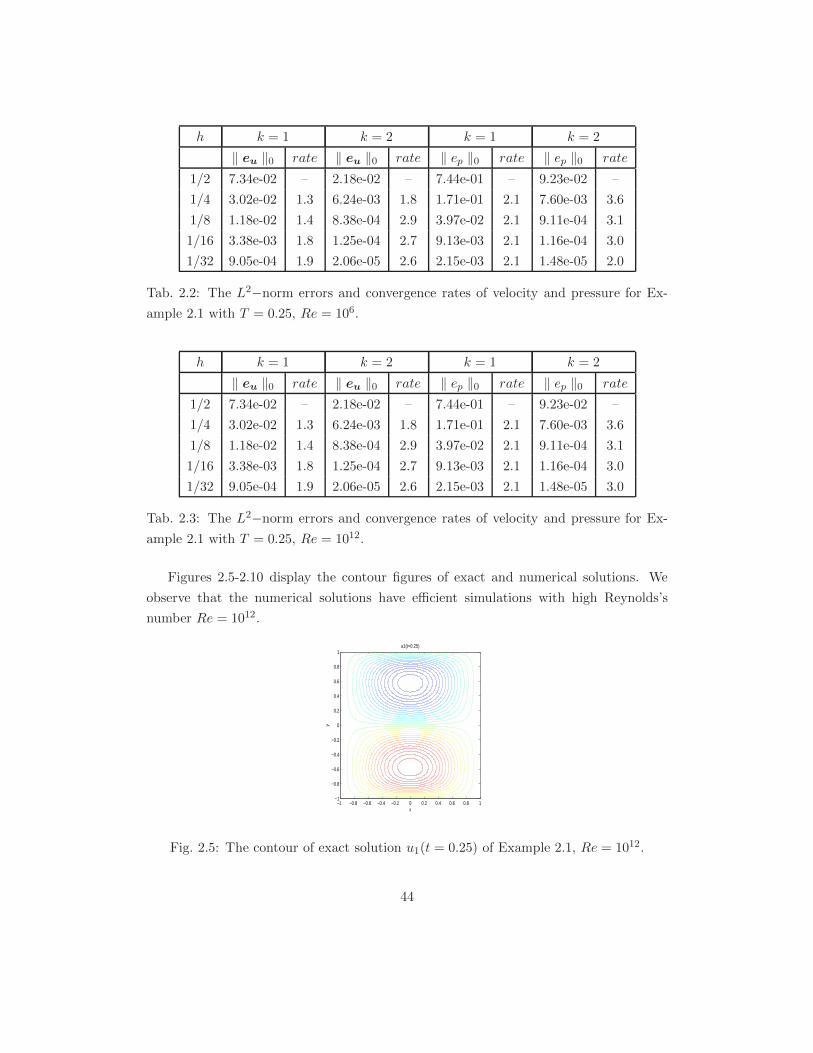
h k = 1 k = 2 k = 1 k = 2


1/2 7.34e-02 – 2.18e-02 – 7.44e-01 – 9.23e-02 –

1/4 3.02e-02 1.3 6.24e-03 1.8 1.71e-01 2.1 7.60e-03 3.6

1/8 1.18e-02 1.4 8.38e-04 2.9 3.97e-02 2.1 9.11e-04 3.1

1/16 3.38e-03 1.8 1.25e-04 2.7 9.13e-03 2.1 1.16e-04 3.0

1/32 9.05e-04 1.9 2.06e-05 2.6 2.15e-03 2.1 1.48e-05 2.0


ample 2.1 with T = 0.25, Re = 106.

h k = 1 k = 2 k = 1 k = 2


1/2 7.34e-02 – 2.18e-02 – 7.44e-01 – 9.23e-02 –

1/4 3.02e-02 1.3 6.24e-03 1.8 1.71e-01 2.1 7.60e-03 3.6

1/8 1.18e-02 1.4 8.38e-04 2.9 3.97e-02 2.1 9.11e-04 3.1

1/16 3.38e-03 1.8 1.25e-04 2.7 9.13e-03 2.1 1.16e-04 3.0

1/32 9.05e-04 1.9 2.06e-05 2.6 2.15e-03 2.1 1.48e-05 3.0


ample 2.1 with T = 0.25, Re = 1012.

Figures 2.5-2.10 display the contour figures of exact and numerical solutions. We

observe that the numerical solutions have efficient simulations with high Reynolds’s

number Re = 1012.

x

y

u1(t=0.25)

−1 −0.8 −0.6 −0.4 −0.2 0 0.2 0.4 0.6 0.8 1−1

−0.8

−0.6

−0.4

−0.2

0

0.2

0.4

0.6

0.8

1

Fig. 2.5: The contour of exact solution u1(t = 0.25) of Example 2.1, Re = 1012.

44

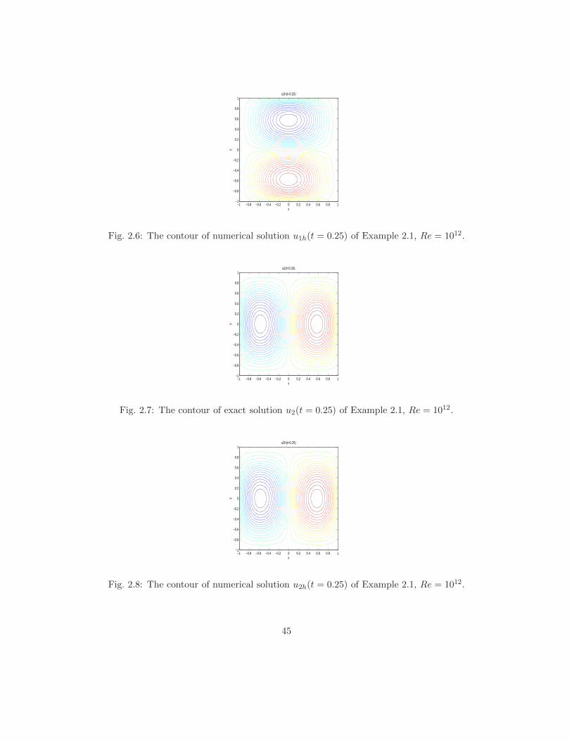
x

y

u1h(t=0.25)

−1 −0.8 −0.6 −0.4 −0.2 0 0.2 0.4 0.6 0.8 1−1

−0.8

−0.6

−0.4

−0.2

0

0.2

0.4

0.6

0.8

1

Fig. 2.6: The contour of numerical solution u1h(t = 0.25) of Example 2.1, Re = 1012.

x

y

u2(t=0.25)

−1 −0.8 −0.6 −0.4 −0.2 0 0.2 0.4 0.6 0.8 1−1

−0.8

−0.6

−0.4

−0.2

0

0.2

0.4

0.6

0.8

1

Fig. 2.7: The contour of exact solution u2(t = 0.25) of Example 2.1, Re = 1012.

x

y

u2h(t=0.25)

−1 −0.8 −0.6 −0.4 −0.2 0 0.2 0.4 0.6 0.8 1−1

−0.8

−0.6

−0.4

−0.2

0

0.2

0.4

0.6

0.8

1


45

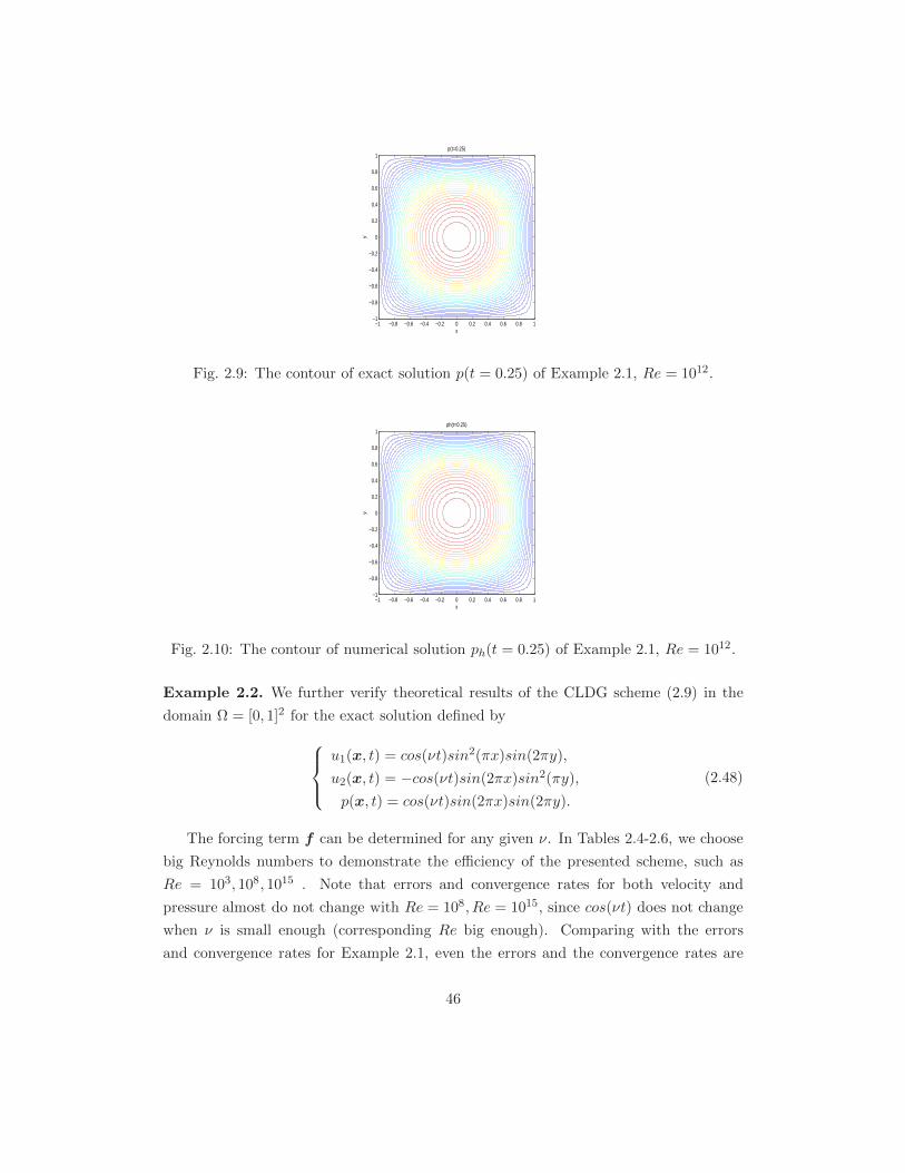
x

y

p(t=0.25)

−1 −0.8 −0.6 −0.4 −0.2 0 0.2 0.4 0.6 0.8 1−1

−0.8

−0.6

−0.4

−0.2

0

0.2

0.4

0.6

0.8

1

Fig. 2.9: The contour of exact solution p(t = 0.25) of Example 2.1, Re = 1012.

x

y

ph(t=0.25)

−1 −0.8 −0.6 −0.4 −0.2 0 0.2 0.4 0.6 0.8 1−1

−0.8

−0.6

−0.4

−0.2

0

0.2

0.4

0.6

0.8

1

Fig. 2.10: The contour of numerical solution ph(t = 0.25) of Example 2.1, Re = 1012.

Example 2.2. We further verify theoretical results of the CLDG scheme (2.9) in the

domain Ω = [0, 1]2 for the exact solution defined by

u1(x, t) = cos(νt)sin2(πx)sin(2πy),

u2(x, t) = −cos(νt)sin(2πx)sin2(πy),p(x, t) = cos(νt)sin(2πx)sin(2πy).

(2.48)

The forcing term f can be determined for any given ν. In Tables 2.4-2.6, we choose

big Reynolds numbers to demonstrate the efficiency of the presented scheme, such as

Re = 103, 108, 1015 . Note that errors and convergence rates for both velocity and

pressure almost do not change with Re = 108, Re = 1015, since cos(νt) does not change

when ν is small enough (corresponding Re big enough). Comparing with the errors

and convergence rates for Example 2.1, even the errors and the convergence rates are

46

not as good as Example 2.1, they still coincide with theoretical results. In order to

further observe the simulations of numerical solutions, we compare the figures of exact

and numerical solutions with Re = 1015 in Figures 2.11-2.16.

h k = 1 k = 2 k = 1 k = 2


1/4 8.15e-02 – 4.63e-02 – 2.11e-01 – 3.26e-02 –

1/8 3.88e-02 1.1 4.51e-03 3.4 4.17e-02 2.3 6.10e-03 2.4

1/16 1.35e-02 1.5 5.67e-04 3.0 9.89e-02 2.1 1.05e-03 2.5

1/32 5.45e-03 1.3 1.01e-04 2.5 4.37e-03 1.2 2.34e-04 2.2


ample 2.2 with T = 0.5, Re = 102.

h k = 1 k = 2 k = 1 k = 2


1/4 1.08e-01 – 1.13e-01 – 2.10e-01 – 4.91e-02 –

1/8 7.65e-02 0.5 1.72e-02 2.7 4.02e-02 2.4 1.29e-02 1.9

1/16 2.95e-02 1.4 2.93e-03 2.6 1.79e-02 1.2 3.17e-03 2.0

1/32 1.33e-02 1.1 1.01e-03 1.5 1.10e-02 0.7 7.38e-04 2.1


ample 2.2 with T = 0.5, Re = 108.

h k = 1 k = 2 k = 1 k = 2


1/4 1.08e-01 – 1.13e-01 – 2.10e-01 – 4.91e-02 –

1/8 7.65e-02 0.5 1.72e-02 2.7 4.02e-02 2.4 1.29e-02 1.9

1/16 2.91e-02 1.4 2.93e-03 2.6 1.80e-02 1.2 3.17e-03 2.0

1/32 1.33e-02 1.1 1.01e-03 1.5 1.10e-02 0.7 7.38e-04 2.1


ample 2.2 with T = 0.5, Re = 1015.

47

0

0.5

1

00.2

0.40.6

0.81

−1

−0.5

0

0.5

1

1.5

x

u1(t=1)

y

z

Fig. 2.11: Exact solution u1(t = 1) of Example 2.2, Re = 1015.

0

0.5

1

00.2

0.40.6

0.81

−1

−0.5

0

0.5

1

1.5

x

u1h(t=1)

y

z

Fig. 2.12: Numerical solution u1h(t = 1) of Example 2.2, Re = 1015.

0

0.5

1

00.2

0.40.6

0.81

−1

−0.5

0

0.5

1

1.5

x

u2(t=1)

y

z

Fig. 2.13: Exact solution u2(t = 1) of Example 2.2, Re = 1015.

48

0

0.5

1

00.2

0.40.6

0.81

−1

−0.5

0

0.5

1

1.5

x

u2h(t=1)

y

z

Fig. 2.14: Numerical solution u2h(t = 1) of Example 2.2, Re = 1015.

0

0.5

1

00.2

0.40.6

0.81

−1

−0.5

0

0.5

1

1.5

x

p(t=1)

y

z

Fig. 2.15: Exact solution p(t = 1) of Example 2.2, Re = 1015.

0

0.5

1

00.2

0.40.6

0.81

−1

−0.5

0

0.5

1

1.5

x

ph(t=1)

y

z

Fig. 2.16: Numerical solution ph(t = 1) of Example 2.2, Re = 1015.

49

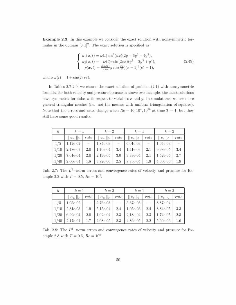
Example 2.3. In this example we consider the exact solution with nonsymmetric for-

mulas in the domain [0, 1]2. The exact solution is specified as

u1(x, t) = ω(t) sin2(πx)(2y − 6y2 + 4y3),

u2(x, t) = −ω(t)π sin(2πx)(y2 − 2y3 + y4),

p(x, t) = ∂tω(t)2πν y cos(πy2 )(x− 1)3(ex − 1),

(2.49)

where ω(t) = 1 + sin(2πνt).

In Tables 2.7-2.9, we choose the exact solution of problem (2.1) with nonsymmetric

formulas for both velocity and pressure because in above two examples the exact solutions

have symmetric formulas with respect to variables x and y. In simulations, we use more

general triangular meshes (i.e. not the meshes with uniform triangulation of squares).

Note that the errors and rates change when Re = 10, 104, 1016 at time T = 1, but they

still have some good results.

h k = 1 k = 2 k = 1 k = 2


1/5 1.12e-02 – 1.84e-03 – 6.01e-03 – 1.04e-03 –

1/10 2.78e-03 2.0 1.70e-04 3.4 1.41e-03 2.1 9.98e-05 3.4

1/20 7.01e-04 2.0 2.19e-05 3.0 3.33e-04 2.1 1.52e-05 2.7

1/40 2.00e-04 1.8 3.82e-06 2.5 8.83e-05 1.9 4.00e-06 1.9


ample 2.3 with T = 0.5, Re = 102.

h k = 1 k = 2 k = 1 k = 2


1/5 1.05e-02 – 2.76e-03 – 5.37e-03 – 8.87e-04 –

1/10 2.81e-03 1.9 5.15e-04 2.4 1.05e-03 2.4 8.84e-05 3.3

1/20 6.99e-04 2.0 1.02e-04 2.3 2.18e-04 2.3 1.74e-05 2.3

1/40 2.17e-04 1.7 2.08e-05 2.3 4.86e-05 2.2 5.90e-06 1.6


ample 2.3 with T = 0.5, Re = 108.

50

h k = 1 k = 2 k = 1 k = 2


1/5 1.05e-02 – 2.76e-03 – 5.37e-03 – 8.87e-04 –

1/10 2.81e-03 1.9 5.15e-04 2.4 1.05e-03 2.4 8.84e-05 3.3

1/20 6.99e-04 2.0 1.02e-04 2.3 2.18e-04 2.3 1.74e-05 2.3

1/40 2.17e-04 1.7 2.08e-05 2.3 4.86e-05 2.2 5.90e-06 1.6


ample 2.3 with T = 0.5, Re = 1015.

10−2

10−1

100

10−5

10−4

10−3

10−2

10−1

h

err

or

2.01,k=1

2.51,k=2

Fig. 2.17: Error and rate of velocity in Example 2.3, Re = 10.

10−2

10−1

100

10−5

10−4

10−3

10−2

10−1

h

err

or

2.66,k=2

1.79,k=1

Fig. 2.18: Error and rate of pressure in Example 2.3, Re = 10.

51

10−2

10−1

100

10−6

10−5

10−4

10−3

10−2

10−1

h

err

or

1.96,k=1

3.15,k=2


10−2

10−1

100

10−6

10−5

10−4

10−3

10−2

h

err

or

2.32,k=1

2.76,k=2


10−2

10−1

100

10−5

10−4

10−3

10−2

10−1

h

err

or

1.91,k=1

2.38,k=2


52

10−2

10−1

100

10−6

10−5

10−4

10−3

10−2

h

err

or

2.32,k=1

2.26,k=2


Example 2.4. In this example we will consider discontinuous solution in the domain

[−1, 1]2. The exact solution is specified as

u1(x, t) =

−e−4π2νt sin(2πy), if |x| < 0.5, |y| < 0.5,

0, else,

u2(x, t) =

e−4π2νt sin(2πx), if |x| < 0.5, |y| < 0.5,

0, else,

p(x, t) =

e−8π2νt sin(2πx) sin(2πy), if |x| < 0.5, |y| < 0.5,

0, else.

The force function f can be determined by any ν according to the above solution.

In this example, we choose the discontinuous solution to show the advantage of

discontinuous Galerkin method comparing with continuous finite element method that

discontinuous Galerkin method can simulate the discontinuous solutions very well. From

the Figures 2.17-2.22, we give the figures of exact and numerical ones to compare. Note

that the simulations can display the discontinuous parts and separate different values

clearly. Even for the pressure p, it still has a good approximation. Figures 2.23-2.25,

display the contour figures of numerical solutions to validate the efficiency of the CLDG

scheme we proposed.

53

h k = 1 k = 2 k = 1 k = 2

‖ eu ‖0 ‖ eu ‖0 ‖ ep ‖0 ‖ ep ‖01/4 2.93e-01 3.65e-01 6.08e-01 5.06e-01

1/8 3.37e-01 3.69e-01 5.11e-01 4.50e-01

1/16 3.59e-01 3.73e-01 4.73e-01 4.23e-01

1/32 3.68e-01 3.74e-01 4.60e-01 4.11e-01


ample 2.4 with T = 0.05, Re = 102.

h k = 1 k = 2 k = 1 k = 2

‖ eu ‖0 ‖ eu ‖0 ‖ ep ‖0 ‖ ep ‖01/4 2.99e-01 3.71e-01 6.31e-01 5.25e-01

1/8 3.42e-01 3.77e-01 5.33e-01 4.70e-01

1/16 3.66e-01 3.80e-01 4.89e-01 4.43e-01

1/32 3.75e-01 3.81e-01 4.60e-01 4.30e-01

Tab. 2.11: The L2−norm errors of velocity and pressure for Example 2.4 with T = 0.05,

Re = 108.

Fig. 2.23: Exact solution u1(t = 0.01) of Example 2.4, Re = 108.

54

Fig. 2.24: Numerical solution u1h(t = 0.01) of Example 2.4, Re = 108.

Fig. 2.25: Exact solution u2(t = 0.01) of Example 2.4, Re = 108.

Fig. 2.26: Numerical solution u2h(t = 0.01) of Example 2.4, Re = 108.

55

Fig. 2.27: Exact solution p(t = 0.01) of Example 2.4, Re = 108.

Fig. 2.28: Numerical solution ph(t = 0.01) of Example 2.4, Re = 108.

u1h(t=0.05)

−1 −0.5 0 0.5 1−1

−0.8

−0.6

−0.4

−0.2

0

0.2

0.4

0.6

0.8

1

−0.8

−0.6

−0.4

−0.2

0

0.2

0.4

0.6

0.8


56

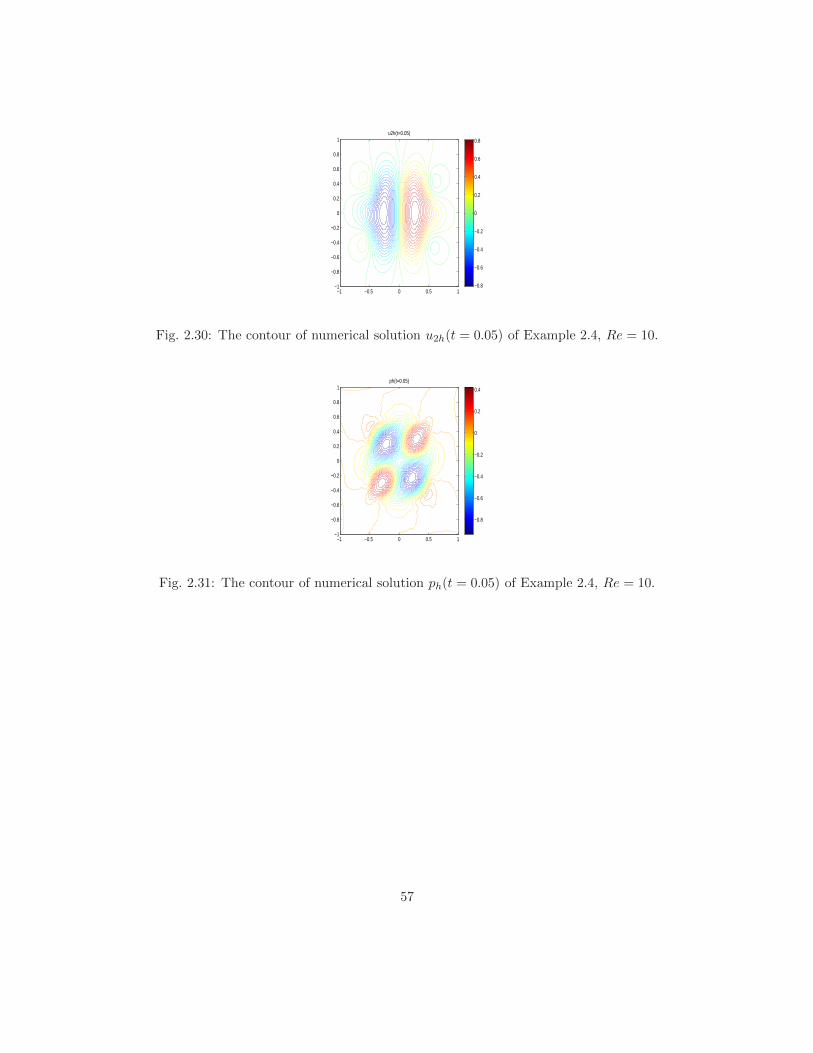
u2h(t=0.05)

−1 −0.5 0 0.5 1−1

−0.8

−0.6

−0.4

−0.2

0

0.2

0.4

0.6

0.8

1

−0.8

−0.6

−0.4

−0.2

0

0.2

0.4

0.6

0.8


ph(t=0.05)

−1 −0.5 0 0.5 1−1

−0.8

−0.6

−0.4

−0.2

0

0.2

0.4

0.6

0.8

1

−0.8

−0.6

−0.4

−0.2

0

0.2

0.4

Fig. 2.31: The contour of numerical solution ph(t = 0.05) of Example 2.4, Re = 10.

57

Chapter 3

HDG method for fractional

convection-diffusion equations

3.1 Fractional convection-diffusion problem

Here, we shall consider time-dependent space-fractional convection-diffusion problem for

u in the form:

∂tu+ b · ∇u− c1∂αu∂xα − c2

∂βu∂yβ

= f, (x, t) ∈ Ω× J,

u(x, t) = 0, (x, t) ∈ ∂Ω× J,

u(x, 0) = u0(x), x ∈ Ω,

(3.1)

where Ω = (a, b) × (c, d) and J = [0, T ] with the superdiffusion operators defined by

operators ∂αu∂xα and ∂βu

∂yβ, 1 < α, β ≤ 2. The function f(x, t) ∈ L2(J ;L2(Ω)) is a source

term, the diffusion coefficients c1 and c2 are supposed to be positive constants, the con-

vection coefficient b(x, t) is bounded vector function, and the solution u is also supposed

to satisfy u ∈ L∞(J ;H2(Ω)), ∂tu ∈ L2(J ;H1(Ω)), ∂ttu ∈ L2(J ;L2(Ω)), u0 ∈ L2(Ω).

3.2 Fractional norms in variational norms

Lemma 3.1. [26, 59] Suppose that u(x) is a function defined in the interval (a, b). If

u(k)(x) = 0, when x = a or x = b, ∀ 0 ≤ k ≤ n− 1, then for n− 1 < ν < n, n ∈ N+, the

58

following hold

aDνxu(x) = Dn

aIn−νx u(x) =aIn−νx

(Dnu(x)

),

xDνb u(x) = (−D)nxIn−νb u(x) =xIn−νb

((−D)nu(x)

).

Note that, from Definition 1.2, Definition 1.3 and Lemma 3.1 if the solution u of

(3.1) satisfies u(k)(x, y) = 0, k = 0, 1 when x = a or y = c, then for any 1 < α, β ≤ 2,

the fractional derivatives of function u(x, y) on Ω = (a, b) × (c, d) can be rewritten as (

see [47, 59]):

∂αu

∂xα=

∂2

∂x2aI2−αx u(x, y) =

∂

∂xaI2−αx

( ∂∂xu(x, y)

)= aI2−α

x

( ∂2∂x2

u(x, y)), (3.2)

∂βu

∂yβ=

∂2

∂y2cI2−βy u(x, y) =

−∂∂y

cI2−βy

(−∂∂y

u(x, y))= cI2−β

y

( ∂2∂y2

u(x, y)). (3.3)

Definition 3.1. [26](The left and right fractional spaces

)For 0 < µ < 1, extend u(x)

outside of I := (a, b) by zero. Then define the norm

‖ u ‖J−µL (R) :=‖−∞Iµxu ‖L2(R), (3.4)

‖ u ‖J−µR (R) :=‖xIµ∞u ‖L2(R) . (3.5)

Let the two spaces J−µL (R) and J−µ

R (R) denote the closures of C∞0 (R) with respect

to ‖ · ‖J−µL

and ‖ · ‖J−µR

, respectively.

Lemma 3.2. [26, 28, 59] For µ > 0, assume that u(x) is a real function. Then

(−∞Iµxu,xIµ∞) = cos(µπ) ‖ u ‖2J−µL (R)= cos(µπ) ‖ u ‖2

J−µR (R) . (3.6)

Generally, we consider the case in which the problem in a bounded domain instead

of R. Then, we restrict the definitions to I = (a, b).

Definition 3.2. [26, 59] Define the spaces J−µL,0(I) and J

−µR,0(I) as the closures of C

∞0 (I)

under their norms.

Theorem 3.3. [26, 59] If −µ2 < −µ1 < 0, then J−µ1L,0 (I) and J−µ1

R,0 (I) are embedded

into J−µ2L,0 (I) and J−µ2

R,0 (I), respectively. Furthermore, L2(I) is embedded into both of

59

them.

Definition 3.3. [26, 59] By Lemma 1, Lemma 3.2, Definition 3.1 and Definition 3.2,

there are

∫ d

c(aI2−α

x u(·, y), u(·, y))L2(a,b)dy = cos(α1π)

∫ d

c‖u(·, y)‖2

J−α1R,0 (a,b)

dy, (3.7)

∫ b

a(cI2−β

y u(x, ·), u(x, ·))L2(c,d)dx = cos(β1π)

∫ b

a‖u(x, ·)‖2

J−β1R,0 (c,d)

dx, (3.8)

where the spaces J−α1R,0 (a, b) and J−β1

R,0 (c, d) are the closures of C∞0 (a, b) and C∞

0 (c, d)

under their norms, respectively, and α1 = 1− α2 , β1 = 1− β

2 , 0 ≤ α1, β1 <12 .

Remark 3.1. It follows from Theorem 3.3 that

∫ d

c‖u(·, y)‖2

J−(2−α)R,0 (a,b)

dy ≤ C

∫ d

c‖u(·, y)‖2

J−α1R,0 (a,b)

dy,

∫ b

a‖u(x, ·)‖2

J−(2−β)R,0 (c,d)

dx ≤ C

∫ b

a‖u(x, ·)‖2

J−β1R,0 (c,d)

dx,

where C is a generic constant.

3.3 Derivation of numerical scheme

We focus on deriving the fully discrete numerical scheme of two dimensional (2D) space-

fractional convection-diffusion equations.

As Ref. [11], let ψ(x, t) = (1 + |b(x, t)|2) 12 , where |b(x, t)|2 = b21 + b22. Hence, the

characteristic direction associated with ∂tu+ b · ∇u is denoted by ∂τ = ∂tψ + b·∇

ψ . Then

the original equation of (3.1) can be rewritten as a mixed form [21, 26, 59]:

ψ∂τu−∇ · σ = f(x, t), (x, t) ∈ Ω× J,

σ − (c1aI2−αx px, c2cI2−β

y py) = 0, (x, t) ∈ Ω× J,

p−∇u = 0, (x, t) ∈ Ω× J,

u(x, t) = 0, (x, t) ∈ ∂Ω× J,

u(x, 0) = u0(x), x ∈ Ω,

(3.9)

60

where aI2−αx and cI2−β

y are fractional operators of Definition 1.1.

For an arbitrary subset E ∈ Eh, we multiply the first, second, and the third equa-

tion of (3.9) by the smooth test functions (v, τ , q), respectively. In order to obtain a

symmetric weak variational formulation, we only integrate the first equation of (3.9) by

parts, and obtain

∫E ψ∂τuvdx+

∫E σ · ∇vdx−

∫∂E σ · nEvds =

∫E fvdx,

∫E σ · τdx−

∫E(c1aI2−α

x px, c2cI2−βy py) · τdx = 0,

∫E p · qdx−

∫E ∇u · qdx = 0,

(3.10)

where nE is the outward unit normal to ∂E. Note that the above equations are well

defined by any functions (u,σ,p) and (v, τ , q) in V ×Q×Q, where

V =u ∈ L2(Ω) : u|E ∈ H1(E), ∀E ∈ Eh

,

Q =p ∈ (L2(Ω))2 : p|E ∈ (H1(E))2, ∀E ∈ Eh

.

Next we will approximate the exact solution (u,σ,p) with the functions (uh,σh,ph) in

the finite element spaces Vh ×Qh ×Qh ⊂ V ×Q×Q, where

Vh =uh ∈ L2(Ω) : uh|E ∈ Pk(E), ∀E ∈ Eh

,

Qh =ph ∈ (L2(Ω))2 : ph|E ∈ (Pk(E))2, ∀E ∈ Eh

,

where the finite element space Pk(E) denotes the set of polynomials of degree less than

or equal to k ≥ 0.

Thus, the approximate solution (uh,σh,ph) satisfies the weak formulation, for all

(v, τ , q) ∈ Vh ×Qh ×Qh such that

∫E ψ∂τuhvdx+

∫E σh · ∇vdx−

∫∂E σ⋆h · nEvds =

∫E fvdx,

∫E σh · τdx−

∫E(c1aI2−α

x pxh, c2 cI2−βy pyh) · τdx = 0,

∫E ph · qdx−

∫E ∇uh · qdx = 0,

(3.11)

61

where the numerical fluxes are well chosen as σ⋆h = σh, ∀e ∈ E Bh in order to ensure

the stability of the scheme and its accuracy.

It is well known that the fluxes σ⋆h = σh are consistent. By inspiration in penalty

Galerkin methods [50], we naturally consider a fact that [u]∣∣e= 0,∀e ∈ E B

h and [σ] =

0,∀e ∈ E ih. Therefore, a symmetric and stable DG scheme is obtained as following.

Substituting the flux σ⋆h = σh into equation (3.11), summing over all the elements,

and adding the penalty terms, we observe that for (uh,σh,ph) ∈ Vh×Qh×Qh, the semi-

discrete variational formulation is given by

(ψ∂τuh, v

)+ (σh,∇v)− (σh · ne, [v])E B

h+ ǫ1([uh], [v])E B

h= (f, v),

(σh, τ ) −((c1aI2−α

x pxh, c2cI2−βy pyh), τ

)= 0,

(ph, q)− (∇uh, q) + ([uh], q · ne)E Bh+ ǫ2([σh], [q])E i

h= 0.

(3.12)

For any (v, τ , q) ∈ Vh × Qh × Qh, the exact solution of (3.1) is expected to be at

least continuous and differentiable, which keeps the consistency of the scheme. The term

([u], q·ne)E Bh

vanishes since the exact solution u satisfies [u]∣∣e= 0,∀e ∈ E B

h . Note that

ǫ1([u], [v])E Bh

penalizes the jump in the function u, whereas ǫ2([σ], [q])E ihpenalizes the

jump in the function σ. Here ǫ1 and ǫ2 are chosen as positive numbers. Unfortunately

the third equation of (3.12) loses the locality of discontinuous Galerkin method. Since

ph is function of uh and σh, ph can not be eliminated from the third equation. Finally

we have to obtain three unknowns uh, pxh, pyh to be solved. Although such mixed DG

method does not eliminate many unknowns of the hybridized DG method, our choice of

fluxes makes the error analysis available.

Above and throughout this chapter, we use the notations

(w, v) =∑

E∈Eh

(w, v)E , (w, v)E ih=∑

e∈E ih

(w, v)e, (w, v)E Bh

=∑

e∈EBh

(w, v)e.

3.3.1 Dealing with time

We now discretize the time derivative with the method of characteristics based on hy-

bridized discontinuous Galerkin method.

For each positive integer N , let 0 = t0 < t1 < · · · < tN = T be a uniform partition

of J into subintervals Jn = (tn−1, tn] with time step ∆t = tn − tn−1, 1 ≤ n ≤ N . The

characteristic tracing back along the field b of a point x ∈ Ω at time tn to tn−1 is

62

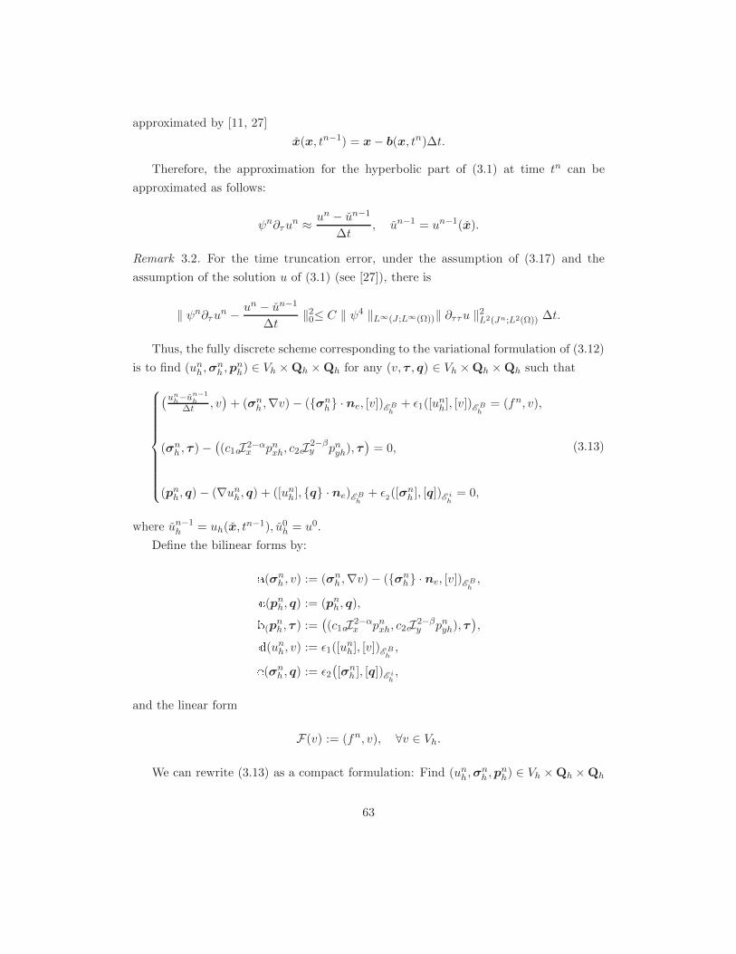
approximated by [11, 27]

x(x, tn−1) = x− b(x, tn)∆t.

Therefore, the approximation for the hyperbolic part of (3.1) at time tn can be

approximated as follows:

ψn∂τun ≈ un − un−1

∆t, un−1 = un−1(x).

Remark 3.2. For the time truncation error, under the assumption of (3.17) and the

assumption of the solution u of (3.1) (see [27]), there is

‖ ψn∂τun −un − un−1

∆t‖20≤ C ‖ ψ4 ‖L∞(J ;L∞(Ω))‖ ∂ττu ‖2L2(Jn;L2(Ω)) ∆t.

Thus, the fully discrete scheme corresponding to the variational formulation of (3.12)

is to find (unh,σnh ,p

nh) ∈ Vh ×Qh ×Qh for any (v, τ , q) ∈ Vh ×Qh ×Qh such that

(unh−un−1h

∆t , v)+ (σnh ,∇v)− (σnh · ne, [v])E B

h+ ǫ1([u

nh], [v])E B

h= (fn, v),

(σnh , τ )−((c1aI2−α

x pnxh, c2cI2−βy pnyh), τ

)= 0,

(pnh, q)− (∇unh, q) + ([unh], q · ne)E Bh+ ǫ2([σ

nh ], [q])E i

h= 0,

(3.13)

where un−1h = uh(x, t

n−1), u0h = u0.

Define the bilinear forms by:a(σnh , v) := (σnh ,∇v)− (σnh · ne, [v])E Bh, (pnh, q) := (pnh, q),b(p

nh, τ ) :=

((c1aI2−α

x pnxh, c2cI2−βy pnyh), τ

),d(unh, v) := ǫ1([u

nh], [v])E B

h,e(σnh , q) := ǫ2

([σnh ], [q])E i

h,

and the linear form

F(v) := (fn, v), ∀v ∈ Vh.

We can rewrite (3.13) as a compact formulation: Find (unh,σnh ,p

nh) ∈ Vh ×Qh ×Qh

63

at time t = tn such that

(unh−un−1h

∆t , v)+ a(σnh , v) + d(unh, v) = F(v), ∀v ∈ Vh, (σnh , τ )− b(pnh, τ ) = 0, ∀τ ∈ Qh, (pnh, q) − a(q, unh) + e(σnh , q) = 0, ∀q ∈ Qh.

(3.14)

Now we introduce a semi-norm that appears in the analysis of these schemes, i.e.

∣∣(unh,σnh ,pnh)∣∣2A

= d(unh, unh) + b(pnh,pnh) + e(σnh ,σnh)= c1cos(α1π)

∫ d

c‖ pnxh(·, y) ‖2J−α1

R,0 (a,b)dy + ǫ1

∑

e∈E Bh

‖ [unh] ‖2L2(e)

+ c2cos(β1π)

∫ b

a‖ pnyh(x, ·) ‖2J−β1

R,0 (c,d)dx+ ǫ2

∑

e∈E ih

‖ [σnh ] ‖2L2(e) .

(3.15)

We end this section by showing that (3.13) is uniquely solvable for the solution

(unh,σnh ,p

nh) at each time step n.

Lemma 3.4. (well posedness of the HDG scheme). The HDG method of (3.13) defines

a unique approximation solution (unh,σnh ,p

nh) ∈ Vh ×Qh ×Qh.

Proof. As (3.13) represents a finite system of linear equations, it is enough to show that

the unique solution to (3.13) with f = 0, un−1h = 0.

Indeed, taking v = unh, τ = −pnh, q = σnh into the equations of (3.13), and adding the

equations, we get1

∆t‖ unh ‖20 +

∣∣(unh,σnh ,pnh)∣∣2A = 0, (3.16)

which implies unh = 0,pnh = 0, [σnh ] = 0 on E ih. Next we go back to the second equation

of (3.13) and take τ = σnh , then

‖ σnh ‖20= 0.

Hence, σnh = 0, which completes the proof of the uniqueness of the solution.

64

3.4 Stability analysis and error analysis

3.4.1 Stability analysis

In the following, C indicates a generic constant independent of h and ∆t, which takes

different values in different occurrences.

Throughout this chapter we assume that

b ∈ L∞(J ;W 1,∞(Ω)2). (3.17)

Lemma 3.5. [11] Under (3.17), for any function v ∈ L2(Ω) there is

‖ v ‖20 − ‖ v ‖20≤ C∆t ‖ v ‖20, (3.18)

where v(x) = v(x− b(x, tn)∆t).

Theorem 3.6. (Numerical stability) Let (unh,σnh ,p

nh) satisfy (3.13). With (3.17), the

scheme is stable for (3.13), i.e., for any integers N = 1, 2, · · · , there is

‖ uNh ‖20 +2∆tN∑

n=1


≤ C∆t

N∑

n=1

‖ fn ‖20 +C ‖ u0h ‖20,(3.19)

where the semi-norm | · |A is defined by formula (3.15), and u0h = u0.

Proof. Let v = 2∆tunh, τ = −2∆tpnh, q = 2∆tσnh in equations of (3.14), respectively. By

the symmetry of the bilinear forms, adding the above equations we obtain

2∆tF(unh) = 2∆tb(pnh,pnh) + 2∆te(σnh ,σnh)+ 2(unh − un−1

h , unh)+ 2∆td(unh, unh).

It follows from

2(unh − un−1

h , unh)≥‖ unh ‖20 − ‖ un−1

h ‖20,

65

the Young’s inequality, the definition of F and | · |A, Lemma 3.5 that

‖ unh ‖20 − ‖ un−1h ‖20 +2∆t


≤ C∆t ‖ un−1h ‖20 +∆t

(‖ unh ‖20 + ‖ fn ‖20

).

Summing from n = 1, 2, · · · , N , we get

‖ uNh ‖20 +2∆tN∑

n=1


≤ C∆t

N∑

n=1

‖ unh ‖20 +(1 + C∆t) ‖ u0h ‖20 +∆t

N∑

n=1

‖ fn ‖20 .

Using the discrete Gronwall inequality, with C∆t < 1, ∀N ≥ 1, there is

‖ uNh ‖20 +2∆t

N∑

n=1


≤ C ‖ u0h ‖20 +C∆tN∑

n=1

‖ fn ‖20 .(3.20)

3.4.2 Error analysis

In this subsection we state and discuss error bounds for the HDG method. The main

steps of our error analysis follow Galerkin orthogonality property. As usual, we denote

the error (enu,enσ ,e

np) = (un − unh,σ

n − σnh ,pn − pnh) by the following

(enu,enσ ,e

np) = (un −Πun,σn −Πσn,pn −Πpn) + (Πenu,Πenσ ,Πenp),

where Π and Π = (Π,Π) are linear continuous projection operators from V and Q onto

the finite element spaces Vh and Qh, respectively.

From equation (3.14), we obtain a compact form as follows:

(unh − un−1h

∆t, v)+A(unh,σ

nh ,p

nh; v, τ , q) = F(v), (3.21)

66

by setting

A(unh,σnh ,p

nh; v, τ , q)

= a(σnh , v) + d(unh, v) + (σnh , τ ) − b(pnh, τ )+ (pnh, q)− a(q, unh) + e(σnh , q). (3.22)

Lemma 3.7. Let u ∈ L∞(J ;H2(Ω)), ∂tu ∈ L2(J ;H1(Ω)), ∂ttu ∈ L2(J ;L2(Ω)). Let Π

and Π be linear continuous projection operators from V and Q onto the finite element

spaces Vh and Qh, respectively. Then

(ψn∂τu

n − unh − un−1h

∆t,Πenu

)+∣∣(Πenu,Πenσ ,Πenp)

∣∣2A

= A(Πun − un,Πσn − σn,Πpn − pn; Πenu,−Πenp,Πenσ

).

(3.23)

Proof. Because of the consistency of the numerical fluxes, the exact solution (u,σ,p)

satisfies equation (3.12) and the approximation solution (unh,σnh ,p

nh) satisfies (3.13).

Then, subtracting (3.13) from (3.12) and taking v = Πenu, τ = −Πenp, q = Πenσ, the

error satisfies

(ψn∂τu


∆t,Πenu

)+A

(enu,e

nσ ,e

np; Πe

nu,−Πenp,Πenσ

)= 0, (3.24)

and

∣∣(Πenu,Πenσ ,Πenp)∣∣2A = A

(Πenu,Πenσ ,Πenp; Πe

nu,−Πenp,Πenσ

). (3.25)

By Galerkin orthogonality, there is

A(enu,e

nσ,e

np; Πe

nu,−Πenp,Πenσ

)

= A(Πenu,Πenσ ,Πenp; Πe

nu,−Πenp,Πenσ

)

−A(Πun − un,Πσn − σn,Πpn − pn; Πenu,−Πenp,Πenσ

).

(3.26)

Hence, equation (3.23) follows equalities (3.24), (3.25) and (3.26).

Thus, in order to prove the error bound, all we need to do is to estimate the first

term of the left-side and the right term of equation (3.23), respectively.

The characteristic term

In this subsection, we will estimate the first left-side term of equation (3.23).

67

Lemma 3.8. [11] With (3.17), for any function v ∈ H1(Ω) and each n we have

‖ v − v ‖0≤ C∆t ‖ ∇v ‖0, (3.27)

where v = v(x) = v(x− bn∆t).

The following result is a straightforward consequence of the estimate of the first

left-side term of equation (3.23).

Theorem 3.9. Let u ∈ L∞(J ;H2(Ω)), ∂tu ∈ L2(J ;H1(Ω)), ∂ttu ∈ L2(J ;L2(Ω)) and unhsolve equation (3.13). With (3.17), there is

(ψn∂τu


∆t,Πenu

)

≥ 1

2∆t

(‖ Πenu ‖20 − ‖ Πen−1

u ‖20)− C ‖ Πen−1

u ‖20

− C∆t ‖ ∂ττu ‖2L2(Jn;L2(Ω)) −C

∆t‖ ∂t(Πu− u) ‖2L2(Jn;L2(Ω))

− C ‖ ∇(Πun−1 − un−1) ‖20 −C ‖ Πenu ‖20,

(3.28)

where Π is linear continuous projection operator from V onto the finite element space

Vh.

Proof. From equation (3.23), we observe that

(ψn∂τu


∆t,Πenu

)

=(Πenu −Πen−1

u

∆t,Πenu

)+(ψn∂τu

n − un − un−1

∆t,Πenu

)

−((Πun − un)− (Πun−1 − un−1)

∆t,Πenu

)

=3∑

i=1

Bi.

(3.29)

68

Using Lemma 3.5, we obtain

B1 =(Πenu −Πen−1

u

∆t,Πenu

)

=1

2∆t

(‖ Πenu ‖20 − ‖ Πen−1

u ‖20 + ‖ Πenu −Πen−1u ‖20

)

≥ 1

2∆t

(‖ Πenu ‖20 − ‖ Πen−1

u ‖20)

≥ 1

2∆t

(‖ Πenu ‖20 − ‖ Πen−1

u ‖20)− C ‖ Πen−1

u ‖20,

where Πen−1u = Πun−1 − un−1

h . Also by the Taylor expansion and Holder’s inequality,

| B2 | =∣∣(ψn∂τun −

un − un−1

∆t,Πenu

)∣∣

≤ C∆t ‖ ∂ττu ‖2L2(Jn;L2(Ω)) +C ‖ Πenu ‖20,

and

−B3 =((Πun − un)− (Πun−1 − un−1)

∆t,Πenu

)

=((Πun − un)− (Πun−1 − un−1)

∆t,Πenu

)

+( (Πun−1 − un−1)− (Πun−1 − un−1)

∆t,Πenu

)= S1 + S2,

(3.30)

where

S1 =((Πun − un)− (Πun−1 − un−1)

∆t,Πenu

)

≤ 1

∆t‖ Πenu ‖0

∫ tn

tn−1

‖ ∂t(Πu− u) ‖0 dt

≤ C ‖ Πenu ‖20 +C

∆t‖ ∂t(Πu− u) ‖2L2(Jn;L2(Ω)),

(3.31)

and

S2 =((Πun−1 − un−1)− (Πun−1 − un−1)

∆t,Πenu

)

≤ C ‖ Πenu ‖20 +C ‖ ∇(Πun−1 − un−1) ‖20,(3.32)

follow from Cauchy-Schwarz’s inequality, Young’s inequality and Lemma 3.8. Substitut-

ing B1,B2,B3 into (3.29), we finish the proof.

69

The right hand side term

In this subsection, we will use general analytic methods to get the bound of the right

hand side term of equation (3.23).

Theorem 3.10. Let u be sufficiently smooth and solve (3.9). Assume that (Πun,Πσn

,Πpn) are standard L2-projection operators of (un,σn,pn), and (unh,σnh ,p

nh) solves (3.13).

Under the assumption of (3.17), there is

∣∣∣A(Πun − un,Πσn − σn,Πpn − pn; Πenu,−Πenp,Πenσ

)∣∣∣

≤ Cc1ǫα

∫ d

c‖ Πenpx(·, y) ‖2J−α1

R,0 (a,b)dy + (

C

ǫ1+ Cǫ1)h

2k+1 +C

ǫαh2k+2

+ Cc2ǫβ

∫ b

a‖ Πenpy(x, ·) ‖2J−β1

R,0 (c,d)dx+ (

C

ǫ2+ Cǫ2)h

2k+1 +C

ǫβh2k+2

+ǫ12

∑

e∈EBh

‖ [Πenu] ‖2L2(e) +ǫ22

∑

e∈E ih

‖ [Πenσ] ‖2L2(e) .

(3.33)

Proof. From the definition of A, we have

A(Πun − un,Πσn − σn,Πpn − pn; Πenu,−Πenp,Πenσ

)

≤∣∣a(Πσn − σn,Πenu)

∣∣+∣∣b(Πpn − pn,Πenp)

∣∣+∣∣d(Πun − un,Πenu)

∣∣

+∣∣e(Πσn − σn,Πenσ)

∣∣+∣∣a(Πenσ,Πu

n − un)∣∣+∣∣ (Πσn − σn,−Πenp)

∣∣

+∣∣ (Πpn − pn,Πenσ)

∣∣

=

7∑

i=1

Ti.

(3.34)

Using Holder’s, Young’s inequalities and the property of projection operator Π, from

Lemma 1.6 we obtain

T1 =∣∣a(Πσn − σn,Πenu)

∣∣ =∣∣(Πσn − σn · ne, [Πenu])E B

h

∣∣

≤∑

e∈EBh

‖ Πσn − σn · ne ‖L2(e)‖ [Πenu] ‖L2(e)

≤∑

e∈EBh

( 1ǫ1

‖ Πσn − σn · ne ‖2L2(e) +ǫ14

‖ [Πenu] ‖2L2(e)

)

≤ C

ǫ1h2k+1 +

ǫ14

∑

e∈EBh

‖ [Πenu] ‖2L2(e) .

70

From the property of projection operator Π and Lemma 1, Definition 3.1, Definition 3.3,

Theorem 3.3, it follows that

T2 =∣∣c1(Πpnx − pnx, xI2−α

b Πenpx) + c2(Πpny − pny , yI2−β

d Πenpy)∣∣

≤ c1 ‖ Πpnx − pnx ‖0( ∫ d

c‖ Πenpx(·, y) ‖2J−(2−α)

R,0 (a,b)dy) 1

2

+ c2 ‖ Πpny − pny ‖0( ∫ b

a‖ Πenpy(x, ·) ‖2J−(2−β)

R,0 (c,d)dx) 1

2

≤ Cc1 ‖ Πpnx − pnx ‖0( ∫ d


R,0 (a,b)dy) 1

2

+ Cc2 ‖ Πpny − pny ‖0( ∫ b


R,0 (c,d)dx) 1

2

≤ C

ǫαh2k+2 + Cc1ǫα

∫ d


R,0 (a,b)dy

+C

ǫβh2k+2 + Cc2ǫβ

∫ b


R,0 (c,d)dx,

where ǫα and ǫβ are chosen as sufficiently small numbers such that Cǫα ≤ cos(α1π) and

Cǫβ ≤ cos(β1π).

With the same deduction of T1, there is

T3 =∣∣d(Πun − un,Πenu)

∣∣

≤ ǫ1∑

e∈EBh

(‖ [Πun − un] ‖2L2(e) +

1

4‖ [Πenu] ‖2L2(e)

)

≤ Ch2k+1ǫ1 +ǫ14

∑

e∈EBh

‖ [Πenu] ‖2L2(e) .

By Lemma 1.6, there is

T4 =∣∣e(Πσn − σn,Πenσ)

∣∣

≤ ǫ2∑

e∈E ih

‖ [Πσn − σn] ‖L2(e)‖ [Πenσ] ‖L2(e)

≤ ǫ2∑

e∈E ih

(‖ [Πσn − σn] ‖2L2(e) +

1

4‖ [Πenσ] ‖2L2(e)

)

≤ Cǫ2h2k+1 +

ǫ24

∑

e∈E ih

‖ [Πenσ ] ‖2L2(e) .

71

Integrating the first term of a(Πenσ,Πun−un) by parts, and using the orthogonal prop-

erty of projection operator Π, we get

T5 =∣∣a(Πenσ,Πu

n − un)∣∣

=∣∣([Πenσ], Πun − unne

)E ih

∣∣

≤∑

e∈E ih

‖ [Πenσ] ‖L2(e)‖ Πun − unne ‖L2(e)

≤∑

e∈E ih

( 1ǫ2

‖ Πun − unne ‖2L2(e) +ǫ24

‖ [Πenσ ] ‖2L2(e)

)

≤ C

ǫ2h2k+1 +

ǫ24

∑

e∈E ih

‖ [Πenσ ] ‖2L2(e) .

Note that T6 and T7 vanish because of the orthogonal property of projection Π.

Substituting Ti, i = 1, · · · , 7 into (3.34), we complete the proof.

Error bound

Assume that the corresponding analytical solution is sufficiently regular and satisfies

u ∈ L∞(J ;H2(Ω)), ∂tu ∈ L2(J ;H1(Ω)), ∂ttu ∈ L2(J ;L2(Ω)).

Theorem 3.11. Let (un,σn,pn) be the exact solution of (3.9), and (unh,σnh ,p

nh) be

numerical solution of the HDG scheme corresponding to equation (3.13). Under the

assumption of (3.17), for any integer N = 1, 2, · · · , the following inequality holds

‖ uN − uNh ‖20 +∆tN∑

n=1

(ǫ1∑

e∈EBh

‖ [un − unh] ‖2L2(e) +ǫ2∑

e∈E ih

‖ [σn − σnh ] ‖2L2(e)

)+ 2∆t

N∑

n=1

c1Kα

∫ d

c‖ (pnx − pnxh)(·, y) ‖

2

J−α1R,0 (a,b)

dy

+ 2∆t

N∑

n=1

c2Kβ

∫ b

a‖ (pny − pnyh)(x, ·) ‖

2

J−β1R,0 (c,d)

dx

≤ C(∆t)2N∑

n=1

‖ ∂ττu ‖2L2(Jn;L2(Ω)) +CN∑

n=1

‖ ∂t(Πu− u) ‖2L2(Jn;L2(Ω))

+ Cǫh2k+1 + C∆t

N∑

n=1

| Πun−1 − un−1 |21,

(3.35)

where Kα = cos(α1π) − Cǫα ≥ 0,Kβ = cos(β1π) − Cǫβ ≥ 0, Cǫ is dependent of ǫ1, ǫ2,

72

and ǫα and ǫβ are chosen as above.

Remark 3.3. Note that Cǫ = Cǫ1 +Cǫ1

+Cǫ2 +Cǫ2

is independent on h for some suitable

choices of ǫ1, ǫ2. But if ǫ1 = ǫ2 = h−1, then Cǫ = O(h−1) (see next section).

Proof. Substituting the results of Theorem 3.9 and Theorem 3.10 into equation (3.23),

there is

1

2∆t

(‖ Πenu ‖20 − ‖ Πen−1

u ‖20)+ǫ12

∑

e∈E Bh

‖ [Πenu] ‖2L2(e) +ǫ22

∑

e∈E ih

‖ [Πenσ] ‖2L2(e)

+ c1(cos(α1π)− Cǫα)

∫ d


R,0 (a,b)dy

+ c2(cos(β1π)− Cǫβ)

∫ b


R,0 (c,d)dx

≤ C ‖ Πen−1u ‖20 +C ‖ Πenu ‖20 +C∆t ‖ ∂ττu ‖2L2(Jn;L2(Ω))

+C

∆t‖ ∂t(Πu− u) ‖2L2(Jn;L2(Ω)) +C | Πun−1 − un−1 |21 +Cǫh2k+1.

With Πe0u = 0, multiplying the above inequality by 2∆t for both sides, summing over n

from 1 to N , and using the discrete Gronwall inequality, we obtain

‖ ΠeNu ‖20 +∆t

N∑

n=1

(ǫ1∑

e∈EBh

‖ [Πenu] ‖2L2(e) +ǫ2∑

e∈E ih

‖ [Πenσ] ‖2L2(e)

)

+ 2∆t

N∑

n=1

c1(cos(α1π)− Cǫα)

∫ d


R,0 (a,b)dy

+ 2∆t

N∑

n=1

c2(cos(β1π)− Cǫβ)

∫ b


R,0 (c,d)dx

≤ C(∆t)2N∑

n=1

‖ ∂ττu ‖2L2(Jn;L2(Ω)) +CN∑

n=1

‖ ∂t(Πu− u) ‖2L2(Jn;L2(Ω))

+ C∆t

N∑

n=1

| Πun−1 − un−1 |21 +Cǫh2k+1.

(3.36)

By the triangle inequality, we complete the proof.

73

3.5 Numerical experiments

In this section, we shall illustrate numerical performance of our proposed scheme by

numerical simulation of two examples. In the first example, we verify the accuracy of

our scheme with exact smooth solution u combining with fractional Riemann-Liouville

derivatives with respect to x-variable and y-variable, respectively. When computing the

fractional integral part in triangular meshes ( see Figures 3.1-3.2), we use Gauss points

and weights to deal with the terms relating with the fractional operators element-by-

element ( see [48]). Since this part needs more time and memory ( see [41]), we only

used the piecewise linear basis functions to simulate the solutions in triangular meshes.

TABLE 3.1 and TABLE 3.2 illustrate that our scheme has a good convergence order

with piecewise linear basis function. In the second example, Figures 3.3-3.10 justify that

our scheme simulates the solution very well.

0 0.1 0.2 0.3 0.4 0.5 0.6 0.7 0.8 0.9 10

0.1

0.2

0.3

0.4

0.5

0.6

0.7

0.8

0.9

1

x−direction

y−

dire

ctio

n

triangular meshes

Fig. 3.1: All triangles in x-direction affected by Gauss point (denoted by black square).

0 0.1 0.2 0.3 0.4 0.5 0.6 0.7 0.8 0.9 10

0.1

0.2

0.3

0.4

0.5

0.6

0.7

0.8

0.9

1

x−direction

y−

dire

ctio

n

triangular meshes

Fig. 3.2: All triangles in y-direction affected by Gauss point (denoted by black square).

Example 3.1. Consider the two-dimensional space-fractional convection-diffusion prob-

74

lem (3.1) in the unit square Ω = [0, 1]×[0, 1]. The initial condition and the exact solution

are specified as:

u(x, t) = e−tx2(x− 1)2y2(y − 1)2,

u0(x) = x2(x− 1)2y2(y − 1)2,

b(x, t) = (0, 0).

(3.37)

Then the exact solution has the homogeneous boundary value, and the force term

f(x, t) is determined accordingly from (3.1) for given c1, c2. For our numerical simu-

lation, in order to validate stability and accuracy of the presented HDG scheme, we

choose the time-step, ∆t = O(h), used to advance the discrete formulation from tn−1 to

tn, n = 1, 2, · · · , N . The experimental convergence rate is given by

rate =log(‖ u(t)− uh1(t) ‖L2(Eh1

) / ‖ u(t)− uh2(t) ‖L2(Eh2)

)

log(h1/h2).

(α, β) = (1.2, 1.4), ǫ1 = 1, ǫ2 = 1

h ‖ eu ‖0 rate ‖ eu ‖1 rate ‖ ∂xeu ‖0 rate ‖ ∂yeu ‖01/6 2.23e-04 – 1.28e-04 – 2.22e-03 – 6.52e-03

1/8 1.45e-04 1.5 8.12e-05 1.6 1.79e-03 0.8 6.77e-03

1/10 1.03e-04 1.5 5.67e-05 1.6 1.45e-03 1.0 6.86e-03

1/12 7.83e-05 1.5 4.18e-05 1.7 1.16e-03 1.2 6.90e-03

1/14 5.86e-05 1.9 3.21e-05 1.7 9.75e-04 1.1 6.94e-03

1/16 4.27e-05 2.4 2.41e-05 2.2 9.72e-04 0.2 6.98e-03

(α, β) = (1.2, 1.4),ǫ1 = h−1, ǫ2 = h−1


1/8 1.38e-04 1.5 7.95e-05 1.7 1.65e-03 0.8 6.74e-03

1/10 1.02e-04 1.4 6.25e-05 1.1 1.47e-03 0.5 6.88e-03

1/12 7.51e-05 1.7 4.65e-05 1.6 1.25e-03 0.9 6.92e-03

1/14 5.53e-05 2.0 3.47e-05 1.9 9.44e-04 1.8 6.94e-03

1/16 3.72e-05 3.0 2.27e-05 3.2 7.83e-04 1.4 6.95e-03

Tab. 3.1: Errors and convergence orders of Example 3.1 with c1 = Γ(5−α)Γ(6) , c2 = Γ(3−β)

Γ(2) .

Table 3.1 and Table 3.2 display the numerical L2, L1-errors and derivative errors with

respect to x-variable and y-variable, respectively, at t = 0.1. Note that with different

75

choices of ǫ1, ǫ2, the HDG scheme has good errors ( i.e. 10e − 5), and almost has a

convergence of an order 1.5 in L2-norm. The errors and rates of Table 3.2 are better

than Table 3.1.

(α, β) = (1.9, 1.6),ǫ1 = 0.01, ǫ2 = 0.01


1/8 5.88e-05 1.0 3.77e-05 0.9 7.52e-04 1.5 6.66e-03

1/10 4.49e-05 1.2 2.82e-05 1.3 5.23e-04 1.6 6.78e-03

1/12 3.61e-05 1.2 2.26e-05 1.2 4.02e-04 1.4 6.85e-03

1/14 2.98e-05 1.2 1.82e-05 1.4 3.20e-04 1.5 6.90e-03

1/16 2.42e-05 1.6 1.47e-05 1.6 2.63e-04 1.5 6.93e-03

(α, β) = (1.9, 1.6),ǫ1 = h−1, ǫ2 = h−1


1/8 5.06e-05 1.2 2.39e-05 1.4 7.58e-04 1.5 6.67e-03

1/10 3.88e-05 1.2 2.04e-05 0.7 5.43e-04 1.5 6.79e-03

1/12 3.08e-05 1.3 1.72e-05 0.9 4.23e-04 1.4 6.86e-03

1/14 2.39e-05 1.7 1.29e-05 1.9 3.46e-04 1.3 6.90e-03

1/16 1.69e-05 2.6 8.54e-05 3.1 2.79e-04 1.6 6.93e-03

Tab. 3.2: Errors and convergence orders of Example 3.1 with c1 =Γ(2−α)Γ(6) , c2 = Γ(2−β)

Γ(6) .

Example 3.2. In this example, we shall investigate the approximation solution of

problem (3.1). For convenience, we still choose the domain is the unit square Ω =

(0, 1)× (0, 1), and the initial condition, exact solution u, the vector function b are given

by:

u(x, t) =e−tx2(x− 0.5)2(x− 1)2y2(y − 0.5)2(y − 1)2,

u0(x) = x2(x− 0.5)2(x− 1)2y2(y − 0.5)2(y − 1)2,

b(x, t) = ((x− 0.5),−(y − 0.5)).

(3.38)

For the second example, in order to further support the theoretical convergence

and justify the powerful HDG scheme, we give some approximation solutions with the

refining space-step h to compare with exact solutions. It is clear that the exact solution

of Example 3.2 is nonnegative with four hills. In our simulation, our P1-DG solution

recovers the exact solution perfectly with all four hills in coarse meshes.

In these numerical experiments, we choose ∆t = O(h), ǫ1 = ǫ2 = h−1. Figures 3.3-3.6

76

give the exact solution u and the numerical solutions uh based on different space step

h = 14 ,

18 ,

116 at t = 0.05, α = 1.2,β = 1.4, c1 = Γ(5−α)

Γ(6) , c2 =Γ(3−β)Γ(2) . Figures 3.7-3.10 give

the exact solution u and the numerical solutions uh based on different space step h = 14 ,

18 ,

116 at t = 0.1, α = 1.9, β = 1.6, c1 = Γ(2−α)

Γ(6) , c2 = Γ(2−β)Γ(6) . Note that the numerical

results display that the approximations are more and more accurate with the refining of

the meshes.

0

0.2

0.4

0.6

0.8

1

0

0.2

0.4

0.6

0.8

1

0

2

4

6

x 10−6

x

u(t=0.05)

y

z

Fig. 3.3: Exact solution u(t = 0.05).

0

0.2

0.4

0.6

0.8

1

0

0.2

0.4

0.6

0.8

1

0

2

4

6

x 10−6

x

uh(t=0.05)

y

z

Fig. 3.4: Numerical solution uh(t = 0.05), h = 14 .

77

0

0.2

0.4

0.6

0.8

1

0

0.2

0.4

0.6

0.8

1

0

2

4

6

x 10−6

x

uh(t=0.05)

y

z


0

0.2

0.4

0.6

0.8

1

0

0.2

0.4

0.6

0.8

1

0

2

4

6

x 10−6

x

uh(t=0.05)

y

z


0

0.2

0.4

0.6

0.8

1 0

0.2

0.4

0.6

0.8

10

2

4

6

x 10−6

y

u(t=0.1)

x

z

Fig. 3.7: Exact solution u(t = 0.1).

78

0

0.2

0.4

0.6

0.8

1 0

0.2

0.4

0.6

0.8

1

0

2

4

6

x 10−6

y

uh(t=0.1)

x

z


0

0.2

0.4

0.6

0.8

1 0

0.2

0.4

0.6

0.8

1

0

2

4

6

x 10−6

y

uh(t=0.1)

x

z


0

0.2

0.4

0.6

0.8

1 0

0.2

0.4

0.6

0.8

10

2

4

6

x 10−6

y

uh(t=0.1)

x

z


79

Chapter 4

Conclusions and perspectives

In this thesis, we finished two work from two areas, i.e., characteristic local discontinuous

Galerkin method for the incompressible Navier-Stokes equations proposed in Chapter 2

and hybridized discontinuous Galerkin method for space-fractional convection-diffusion

equations in 2D shown in Chapter 3, respectively.

• S. Q. Wang, W. H. Deng, J. Y. Yuan, Y. J. Wu, Characteristic local discontinuous

Galerkin method for incompressible Navier-Stokes equations. submitted.

• S. Q. Wang, J. Y. Yuan, W. H. Deng, Y. J. Wu, A hybridized discontinuous

Galerkin method for 2D fractional convection-diffusion equations. submitted.

The first work is concerning on a problem of mathematical physical fluid computa-

tion. In this work we extended the work of local discontinuous Galerkin methods for

the Stokes system [15] with characteristic local discontinuous Galerkin (CLDG) method.

By carefully constructing the numerical fluxes, adding the penalty terms, and using

the method of characteristics to discretize the time derivative and nonlinear convective

term, we design the effective LDG scheme to solve the time-dependent incompressible

Navier-Stokes equations in R2. Besides the general advantages of the LDG scheme, the

proposed scheme is theoretically proved or numerically verified to have the following

benefits: 1) it is symmetric, so easy to do theoretical analysis and numerical computa-

tion; 2) theoretically proved to be nonlinear stable; 3) numerically verified to have the

suboptimal convergence rates; 4) the scheme is efficient for a wide range of Reynolds

numbers, such as Re = 102, 103, 106, 108, 1012, 1015, 1016.

For the characteristic local discontinuous Galerkin method for the incompressible

Navier-Stokes equations, we did not complete all problems of considered equations. In

80

our work, we just recasted the solutions with one time accuracy and obtained suboptimal

convergence by simulating some simple examples. In future work, we will consider com-

bining second order modified characteristics with some discontinuous Galerkin methods

to recast the time-dependent incompressible Navier-Stokes equations. In numerical im-

plementation, the benchmark problem which is fundamental problem in Navier-Stokes

equations will be performed.

The second work focus on numerical analysis and implementation of fractional equa-

tions with discontinuous Galerkin method. By carefully introducing the auxiliary vari-

ables and constructing the numerical fluxes, adding the penalty terms, and using the

method of characteristics to deal with the time derivative and convective term, we design

the effective HDG scheme to solve 2D space-fractional convection-diffusion equations

with triangular meshes. As we know, this work is the first time to deal 2D space-

fractional convection-diffusion equations with triangular mesh by the DG method. The

stability and error analysis are investigated. Besides the general advantages of HDG

method, the presented scheme is proved to have the following benefits: 1) it is symmet-

ric, so easy to deal with fractional operators; 2) theoretically, the stability was proved

more easily; 3) the penalty terms made the error analysis more convenient; 4) numeri-

cally verified to have efficient approximation; 5) the scheme was performed very well in

triangular meshes; 6) it is possible to use this scheme to solve nonlinear equations.

As our knowledge, there are few works on applying discontinuous Galerkin method

for fractional equations in 2D, and much less on fractional equations with complicated

domains. In the future, we will extend the work to some space-fractional equations

in some complicated domains, such as triangle, polygonal domains. As we stated that

we performed the simulations only with P1-DG method (linear piecewise polynomial

approximation) because of the expensive memory and time. In next work, the numeri-

cal performance will be improved up to simulate problems with quadratic piecewise or

cubic piecewise polynomial. I think some other interesting fractional problems will be

considered further.

81

Bibliography

[1] A. Allievi, R. Bermejo, Finite element modified method of characteristics for the

Navier-Stokes equations, Int. J. Numer. Meth. Fluids, 32: 439-464, 2000.

[2] T. Arbogast, C.-S. Huang, A fully mass and volume conserving implementation of a

characteristic method for transport problems, SIAM J. Sci. Comput., 28: 2001-2022,

2006.

[3] T. Arbogast, M. F. Wheeler, A characteristics-mixed finite element method for

advection-dominated transport problems, SIAM J. Numer. Anal., 32: 404-424, 1995.

[4] F. Bassi, S. Rebay, A high-order accurate discontinuous finite element method for

the numerical solution of the compressible Navier-Stokes equations, J. Comput. Phys.,

131: 267-279, 1997.

[5] D. A. Benson, S. W. Wheatcraft, M. M. Meerschaert, The fractional-order governing

equation of Levy motion, Water Resour. Res., 36: 1413-1423, 2000.

[6] K. Boukir, Y. Maday, B. Metivet, E. Razafindrakoto, A high order characteris-

tics/finite element method for the incompressible Navier-Stokes equations, Int. J.

Numer. Meth. Fluids, 25: 1421-1454, 1997.

[7] S. C. Brenner, L. R. Scott, The Mathematical Theory of Finite Element Methods,

third edition, Springer, 2008.

[8] B. A. Carreras, V. E. Lynch, G. M. Zaslavsky, Anomalous diffusion and exit time

distribution of particle tracers in plasma turbulence model, Phys. Plasmas, 8: 5096-

5103, 2001.

[9] P. Castillo, B. Cockburn, I. Perugia, and D. Schotzau, An a priori error analysis of

the local discontinuous Galerkin method for elliptic problems, SIAM J. Numer. Anal.,

38: 1676-1706, 2000.

82

[10] M. H. Chen, W. H. Deng, A second-order numerical method for two-dimensional

two-sided space fractional convection diffusion equation, Appl. Math. Model., 38: 3244-

3259, 2014.

[11] Z. X. Chen, Characteristic mixed discontinuous finite element methods for

advection-dominated diffusion problems, Comput. Meth. Appl. Mech. Engrg., 191:

2509-2538, 2002.

[12] Z. X. Chen, R. E. Ewing, Q. Y. Jiang, and A. M. Spagnuolo, Error analysis for

characteristics-based methods for degenerate parabolic problems, SIAM J. Numer.

Anal., 40: 1491-1515, 2002.

[13] A. J. Chorin, J. E. Marsden, A Mathematical Introduction to Fluid Mechanics,

Springer, 1990.

[14] P. G. Ciarlet, The Finite Element Method for Elliptic Problems, SIAM, 2002.

[15] B. Cockburn, G. Kanschat, D. Schotzau, C. Schwab, Local discontinuous Galerkin

methods for the Stokes system, SIAM J. Numer. Anal., 40: 319-343, 2002.

[16] B. Cockburn, G. Kanschat, D. Schotzau, The local discontinuous Galerkin method

for the Ossen equations, Math. Comp., 73: 569-593, 2003.

[17] B. Cockburn, G. Kanschat, D. Schotzau, A locally conservative LDG method for

the incompressible Navier-Stokes equations, Math. Comp., 74: 1067-1095, 2005.

[18] B. Cockburn, G. Kanschat, D. Schotzau, A note on discontinuous Galerkin

divergence-free solutions of Navier-Stokes equations, J. Sci. Comput., 31: 61-73, 2007.

[19] B. Cockburn, G. E. Karniadakis, C. -W. Shu, The Development of Discontinuous

Galerkin Methods, Springer, 2000.

[20] B. Cockburn, J. Gopalakrishnan, F. -J. Sayas, A projection-based error analysis of

HDG methods, Math. Comp., 79: 1351-1367, 2010.

[21] B. Cockburn, C. -W. Shu, The local discontinuous Galerkin method for time-

dependent convection-diffusion systems, SIAM J. Numer. Anal., 35: 2440-2463, 1998.

[22] B. Cockburn, C. -W. Shu, Runge-Kutta discontinuous Galerkin methods for

convection-dominated problems, J. Sci. Comput., 16: 173-261, 2001.

[23] M. R. Cui, A high-order compact exponential scheme for fractional convection-

diffusion equations, J. Comput. Appl. Math., 255: 404-416, 2014.

83

[24] C. N. Dawson, T. F. Russell and M. F. Wheeler, Some improved error estimates for

the modified method of characteristics, SIAM J. Numer. Anal., 26: 1487-1512, 1989.

[25] W. H. Deng, Finite element method for the space and time fractional Fokker-Plank

equations, SIAM J. Numer. Anal., 47: 204-226, 2008.

[26] W. H. Deng, J. S. Hesthaven, Local discontinuous Galerkin methods for fractional

diffusion equations, ESAIM: M2AN, 47: 1845-1864, 2013.

[27] J. Douglas, JR. and T. F. Russell, Numerical methods for convection-dominated dif-

fusion problems based on combining the method of characteristics with finite element

or finite difference procedures, SIAM J. Numer. Anal., 19: 871-885, 1982.

[28] V. J. Ervin, J. P. Roop, Variational formulation for the stationary fractional advec-

tion dispersion equation, Numer. Meth. Part. D. E., 22: 558-576, 2006.

[29] V. Girault, B. Riviere, M. F. Wheeler, A splitting method using discontinuous

Galerkin for the transient incompressible Navier-Stokes equations, ESAIM: M2AN,

39: 1115-1147, 2005.

[30] V. Girault, P. A. Raviart, Finite Element Approximations for the Navier-Stokes

Equations, Springer-Verlag Berlin Heidelberg, 1979.

[31] J. L. Guermond, J. Shen, On the error estimates for the rotational pressure-

correction projection method, Math. Comp., 73: 1719-1737, 2003.

[32] Y. He, A fully discrete stabilized finite-element method for the time-dependent

Navier-Stokes problem, IMA J. Numer. Anal., 23: 665-691, 2003.

[33] J. S. Hesthaven, T. Warburton, Nodal Discontinuous Galerkin Methods: Algorithms,

Analysis, and Applications, Springer, 2008.

[34] X. Ji, H. Z. Tang, High-order accurate Runge-Kutta (local) discontinuous Galerkin

methods for one- and two-dimensional fractional diffusion equations, Numer. Math.

Theor. Meth. Appl., 5: 333-358, 2012.

[35] J. W. Kirchner, X. H. Feng, C. Neal, Fractal stream chemistry and its implications

for contaminant transport in catchments, Nature, 403: 524-527, 2000.

[36] Y. M. Lin, C. J. Xu, Finite difference/spectral approximations for the time-

fractional diffusion equation, J. Comput. Phys., 225: 1533-1552, 2007.

84

[37] M. E. Liu, Y. X. Ren, H. X. Zhang, A class of fully second order accurate projection

methods for solving the incompressible Navier-Stokes equations, J. Comput. Phys.,

200: 325-346, 2004.

[38] F. Liu, P. Zhuang, V. Anh, I. Turner, K. Burrage, Stability and convergence of the

difference methods for the space-time fractional advection-diffusion equation, Appl.

Math. Comp., 191: 12-20, 2007.

[39] R. L. Magin, Fractional Calculus in Bioengineering, Begell House, 2006.

[40] W. McLean, K. Mustapha, Convergence analysis of a discontinuous Galerkin

method for a sub-diffusion equation, Numer. Algor., 52: 69-88, 2009.

[41] W. McLean, Fast summation by interval clustering for an evolution equation with

memory, SIAM J. Sci. Comput., 34: A3039-A3056, 2012.

[42] K. Mustapha, W. McLean, Superconvergence of a discontinuous Galerkin method

for fractional diffusion and wave equations, SIAM J. Numer. Anal., 51: 491-515, 2013.

[43] K. Mustapha, W. McLean, Piecewise-linear, discontinuous Galerkin method for a

fractional diffusion equation, Numer. Algor., 56: 159-184, 2011.

[44] R. H. Nochetto, J. -H. Pyo, The Gauge-Uzawa finite element method. Part I: The

Navier-Stokes Equations, SIAM J. Numer. Anal., 43: 1043-1068, 2005.

[45] K. B. Oldham, J. Spanier, The Fractional Calculus: Theory and Applications of

Differentiation and Integration to Arbitrary, Academic Press, 1974.

[46] O. Pironneau, On the transport-diffusion algorithm and its applications to the

Navier-Stokes equations, Numer. Math., 38: 309-332, 1982.

[47] I. Podlubny, Fractional Differential Equations, Academic Press, 1999.

[48] L. L. Qiu, W. H. Deng, J. S. Hesthaven, Nodal discontinuous Galerkin methods for

fractional diffusion equations on 2D domain with triangualr meshes. submitted.

[49] W. H. Reed and T. R. Hill, Triangular mesh methods for the neutron transport

equation, Los Alamos Scientific Laboratory report LA-UR-73-479, Los Alamos, NM,

1973.

[50] B. Riviere, Discontinuous Galerkin Methods for Solving Elliptic and Parabolic Equa-

tions: Theory and Implementation, SIAM, 1999.

85

[51] B. Riviere, V. Girault, Discontinuous finite element methods for incompressible

flows on subdomains with non-matching interfaces, Comput. Meth. Appl. Mech. En-

grg., 195: 3274-3292, 2006.

[52] J. Sabatier, O. P. Agrawal, J. A. T. Machado, Advances in Fractional Calculus: The-

oretical Developments and Applications in Physics and Engineering, Springer, 2007.

[53] M. F. Shlesinger, B. J. West, J. Klafter, Levy dynamics of enhanced diffusion:

application to turbulence, Phys. Rev. Lett., 58: 1100-1103, 1987.

[54] Z. Y. Si, X. G. Song, P. Z. Huang, Modified characteristics Gauge-Uzawa finite

element method for time dependent conduction-convection problems, J. Sci. Comput.,

58: 1-24, 2014.

[55] E. Suli, Convergence and nonlinear stability of the Lagrange-Galerkin method for

the Navier-Stokes equations, Numer. Math., 53: 459-483, 1988.

[56] R. Temam, Navier-Stokes Equations: Theory and Numerical Analysis, North-

Holland, Amsterdam, 1984.

[57] K. X. Wang, H. Wang, M. Al-Lawatia, H. X. Rui, A family of characteristic dis-

continuous Galerkin methods for transient advection-diffusion equations and their

optimal-order L2 error estimates, Commun. Comput. Phys., 6: 203-230, 2009.

[58] Z. B. Wang, S. W. Vong, A high-order exponential ADI scheme for two dimensional

time fractional convection-diffusion equations, Comput. Math. Appl., 68: 185-196,

2014.

[59] Q. Xu, J. S. Hesthaven, Discontinuous Galerkin method for fractional convection-

diffusion equations, SIAM J. Numer. Anal., 52: 405-423, 2014.

[60] S. Z. Zhai, X. H. Feng, Y. N. He, An unconditionally stable compact ADI method for

three-dimensional time-fractional convection-diffusion equations, J. Comput. Phys.,

269: 138-155, 2014.

86

m´etodo de galerkin descontínuo para dois problemas de convecc ...

Documents

Transcript of m´etodo de galerkin descontínuo para dois problemas de convecc ...