Maria da Glória Abage de Lima€¦ · Lima, Maria da Glória Abage de Essays on heteroskedasticity...
134
UNIVERSIDADE FEDERAL DE PERNAMBUCO Centro de Ciências Exatas e da Natureza Pós-Graduação em Matemática Computacional Essays on heteroskedasticity Maria da Glória Abage de Lima Tese de Doutorado RECIFE 30 de maio de 2008
Transcript of Maria da Glória Abage de Lima€¦ · Lima, Maria da Glória Abage de Essays on heteroskedasticity...
UNIVERSIDADE FEDERAL DE PERNAMBUCOCentro de Ciências Exatas e da Natureza
Pós-Graduação em Matemática Computacional
Essays on heteroskedasticity
Maria da Glória Abage de Lima
Tese de Doutorado
RECIFE30 de maio de 2008
UNIVERSIDADE FEDERAL DE PERNAMBUCOCentro de Ciências Exatas e da Natureza
Maria da Glória Abage de Lima
Essays on heteroskedasticity
Trabalho apresentado ao Programa de Pós-Graduação emMatemática Computacional do Centro de Ciências Exatase da Natureza da UNIVERSIDADE FEDERAL DE PER-NAMBUCO como requisito parcial para obtenção do graude Doutor em Matemática Computacional.
Orientador: Prof. Dr. Francisco Cribari Neto
RECIFE30 de maio de 2008
Lima, Maria da Glória Abage de
Essays on heteroskedasticity / Maria da Glória Abage de Lima. – Recife : O Autor, 2008. xi, 120 folhas : il., fig., tab. Tese (doutorado) – Universidade Federal de Pernambuco. CCEN. Matemática Computacional, 2008.
Inclui bibliografia e apêndice. 1. Análise de regressão. I. Título.
519.536 CDD (22.ed.) MEI2008-064


A Roberto e Juliana.

Acknowledgements
First of all, I thank God, who has always been a source of strength to me.
I also thank Roberto and Juliana. The love we share is a great source of strength and inspiration.
I am also grateful to my advisor, prof. Francisco Cribari Neto, who was always availableand willing to discuss with me the progresses of the researchactivities that led to the presentdissertation.
I thank my employer, Universidade Federal Rural de Pernambuco, for the support that allowedme to complete the Doctoral Program in Computational Mathematics at UFPE.
I also express gratitute to the following professors: Francisco Cribari Neto, Klaus Leite PintoVasconcellos, Audrey Helen Mariz de Aquino Cysneiros, Francisco José de Azevêdo Cysneirosand Sóstenes Lins. They have greatly contributed to my doctoral education. The commentsmade by professors Klaus Leite Pinto Vasconcellos and Sílvio Melo on a preliminary versionof the Ph.D. dissertation during my qualifying exam were helpful and were greatly appreciated.
I am also grateful to my colleagues Graça, Andréa, Ademakson, Donald and Mirele. I havetruly enjoyed our time together.
I thank my friends at the Statistics Departament at UFPE, whohave always been kind to me.Special thanks go to Valéria Bittencourt, who is efficient, polite and available.
Finally, I would like to thank Angela, who has helped me with the final steps needed to completethe submission of this dissertation to UFPE.
iv

Tudo tem o seu tempo determinado, e há tempo para todo o propósitodebaixo do céu:
—ECLESIASTES (3;1)
Resumo
Esta tese de doutorado trata da realização de inferências nomodelo de regressão linear sobheteroscedasticidade de forma desconhecida. No primeiro capítulo, nós desenvolvemos esti-madores intervalares que são robustos à presença de heteroscedasticidade. Esses estimadoressão baseados em estimadores consistentes de matrizes de covariâncias propostos na literatura,bem como em esquemas bootstrap. A evidência numérica favorece o estimador intervalar HC4.O Capítulo 2 desenvolve uma seqüência corrigida por viés de estimadores de matrizes de co-variâncias sob heteroscedasticidade de forma desconhecida a partir de estimador proposto porQian e Wang (2001). Nós mostramos que o estimador de Qian-Wang pode ser generalizado emuma classe mais ampla de estimadores consistentes para matrizes de covariâncias e que nossosresultados podem ser facilmente estendidos a esta classe deestimadores. Finalmente, no Capí-tulo 3 nós usamos métodos de integração numérica para calcular as distribuições nulas exatasde diferentes estatísticas de testes quasi-t, sob a suposição de que os erros são normalmentedistribuídos. Os resultados favorecem o teste HC4.
Palavras-chave: bootstrap, correção de viés, distribuição exata de estatísticas quasi-t, esti-madores consistentes para a matriz de covariâncias sob heteroscedasticidade, heteroscedastici-dade, intervalos de confiança consistentes sob heteroscedasticidade, testes quasi-t.
vi
Abstract
This doctoral dissertation addresses the issue of performing inference on the parameters thatindex the linear regression model under heteroskedasticity of unknown form. In the first chap-ter we develop heteroskedasticity-robust interval estimators. These are based on differentheteroskedasticity-consistent covariance matrix estimators (HCCMEs) proposed in the liter-ature and also on bootstrapping schemes. The numerical evidence presented favors the HC4interval estimator. Chapter 2 develops a sequence of bias-corrected covariance matrix estima-tors based on the HCCME proposed by Qian and Wang (2001). We show that the Qian-Wangestimator can be generalized into a broad class of heteroskedasticity-consistent covariance ma-trix estimators and that our results can be easily extended to such a class of estimators. Finally,Chapter 3 uses numerical integration methods to compute theexact null distributions of dif-ferent quasi-t test estatistics under the assumption that the errors are normally distributed. Theresults favor the HC4-based test.
Keywords: bias correction, bootstrap, exact distributions of quasi-t statistics, heteroskedastic-ity, heteroskedasticity-consistent covariance matrix estimators (HCCME), heteroskedasticity-consistent interval estimators (HCIE), quasi-t tests
vii
Contents
1 Heteroskedasticity-consistent interval estimators 11.1 Introduction 11.2 The model and some point estimators 31.3 Heteroskedasticity-consistent interval estimators 51.4 Numerical evaluation 71.5 Bootstrap intervals 111.6 Confidence regions 161.7 Concluding remarks 20
2 Bias-adjusted covariance matrix estimators 212.1 Introduction 212.2 The model and covariance matrix estimators 222.3 A new class of bias adjusted estimators 252.4 Variance estimation of linear combinations of the elements of β 292.5 Numerical results 322.6 Empirical illustrations 402.7 A generalization of the Qian–Wang estimator 442.8 Concluding remarks 51
3 Inference under heteroskedasticity: numerical evaluation 523.1 Introduction 523.2 The model and some heteroskedasticity-robust standarderrors 543.3 Variance estimation of linear combinations of the elements of β 563.4 Approximate inference using quasi-t tests 573.5 Exact numerical evaluation 583.6 An alternative standard error 653.7 A numerical evaluation of quasi-t tests based onV1 andV2 683.8 Yet another heteroskedasticity-consistent standard error: HC5 723.9 Concluding remarks 81
4 Conclusions 82
5 Resumo do Capítulo 1 835.1 Introdução 835.2 O modelo e alguns estimadores pontuais 835.3 Estimadores intervalares consistentes sob heteroscedasticidade 85
viii
CONTENTS ix
5.4 Avaliação numérica 865.5 Intervalos bootstrap 875.6 Regiões de confiança 88
6 Resumo do Capítulo 2 906.1 Introdução 906.2 O modelo e estimadores da matriz de covariâncias 906.3 Uma nova classe de estimadores ajustados pelo viés 926.4 Estimação da variância de combinações lineares dos elementos deβ 936.5 Resultados numéricos 956.6 Ilustrações empíricas 976.7 Uma generalização do estimador de Qian–Wang 97
7 Resumo do Capítulo 3 1017.1 Introdução 1017.2 O modelo e alguns erros-padrão robustos sob heteroscedasticidade 1017.3 Estimação da variância de combinações lineares dos elementos deβ 1037.4 Inferência usando testes quasi-t 1047.5 Avaliação numérica exata 1057.6 Um erro-padrão alternativo 1077.7 Avaliação numérica de testes quasi-t baseada emV1 e V2 1087.8 Um outro erro-padrão consistente sob heteroscedasticidade: HC5 109
8 Conclusões 112
A O algoritmo de Imhof 113A.1 Algoritmo de Imhof 113A.2 Caso particular 114A.3 Função ProbImhof 114

List of Figures
3.1 Relative quantile discrepancy plots; n=25; HC0, HC3, HC4,V1 593.2 Relative quantile discrepancy plots; n=50; HC0, HC3, HC4,V1 603.3 Relative quantile discrepancy plots; education data; HC0,HC3,HC4,V1 643.4 Pr(t2 ≤ γ | c′β = η)−Pr(χ2
1 ≤ γ); usingV2(a) for different values ofa 68
3.5 Relative quantile discrepancy plots;V1, V2(a) : a=0,2,10,15 703.6 Relative quantile discrepancy plots; education data; uses HC4,V1, V2 733.7 Relative quantile discrepancy plots; HC3, HC4, HC5 753.8 Relative quantile discrepancy plots; education data; HC3, HC4, HC5 773.9 Pr(t2 ≤ γ | c′β = η)−Pr(χ2
1 ≤ γ); using HC5 with different values ofk 783.10 Pr(t2 ≤ γ | c′β = η)−Pr(χ2
1 ≤ γ); HC5 (differentk); education data 79
x

List of Tables
1.1 Maximal leverages 81.2 Confidence intervals forβ1; balanced design; normal errors 81.3 Confidence intervals forβ1; unbalanced design; normal errors 101.4 Confidence intervals forβ1; unbalanced design; skewed errors 101.5 Confidence intervals forβ1; unbalanced design; fat tailed errors 111.6 Bootstrap confidence intervals forβ1; weighted bootstrap 131.7 Bootstrap confidence intervals forβ1; wild and pairs bootstrap 151.8 Bootstrap confidence intervals forβ1; percentile-t bootstrap 171.9 Maximal leverages 181.10 Confidence regions and confidence intervals forβ1 andβ2 19
2.1 Maximal leverages 332.2 Total relative bias of the OLS variance estimator 332.3 Total relative biases: balanced and unbalanced designs 352.4 Total relative mean squared errors; balanced and unbalanced designs 362.5 Maximal biases; balanced and unbalanced designs 372.6 Maximal biases; uses a sequence of equally espaced points in (0,1) 392.7 Standard errors; first application 412.8 Leverage measures; first application 422.9 Leverage measures; second application 422.10 Standard errors; second application 432.11 Total relative biases for the estimators in the generalized class 492.12 Standard errors; corrected estimators:Ψ
(i)3A, Ψ(i)
4A; first application 50
3.1 Maximal leverages 613.2 Pr(t2 ≤ γ | c′β = η); uses HC0, HC3, HC4,V1 623.3 Leverage measures; education data 633.4 Pr(t2 ≤ γ | c′β = η); education data; uses HC0, HC3, HC4,V1 633.5 Pr(t2 ≤ γ | c′β = η); uses HC3, HC4,V1, V2(0), V2(2) andV2(15) 713.6 Maximal leverages 743.7 Pr(t2 ≤ γ | c′β = η); uses HC3, HC4, HC5 763.8 Pr(t2 ≤ γ | c′β = η); education data; uses HC3, HC4, HC5 783.9 Pr(t2 ≤ γ | c′β = η); uses HC4, HC5 803.10 Null rejection rates of HC4 and HC5 quasi-t tests 80
xi
C 1
Heteroskedasticity-consistent interval estimators
1.1 Introduction
The linear regression model is commonly used by practitioners of many different fields tomodel the dependence of a variable of interest on a set of explanatory variables. The regres-sion parameters are most often estimated by ordinary least squares (OLS). Under the usualassumptions, the resulting estimator is optimal in the class of unbiased and linear estimators; itis also consistent and asymptotically normal. A commonly violated assumption is that knownas homoskedasticity, which states that all error variancesmust be the same. The OLS estimator(OLSE), however, remains unbiased, consistent and asymptotically normal when such an as-sumption does not hold, i.e., under heteroskedasticity. Itis, thus, a valid and useful estimator.The trouble lies in the usual estimator of its covariance matrix, which becomes inconsistentand biased when the error variances are not equal. Asymptotically valid hypothesis testinginference on the regression parameters, however, requiresa consistent estimator for such a co-variance matrix, from which one obtains standard errors andestimated covariances. Severalheteroskedasticity-consistent covariance matrix estimators (HCCMEs) were proposed in theliterature. The most well known estimators are the HC0 (White, 1980), HC2 (Horn, Horn andDuncan, 1975), HC3 (Davidson and MacKinnon, 1993) and HC4 (Cribari–Neto, 2004) esti-mators.1 HC0 was proposed by Halbert White in an influentialEconometricapaper and is themost used estimator in empirical studies. White’s estimator is commonly used by practition-ers, especially by reseachers in economics and finance. His paper had been cited over 4,500times by mid 2007. It is noteworthy, nonetheless, that the covariance matrix estimator proposedby Halbert White is typically considerably biased in finite-samples, especially when the datacontain leverage points (Chesher and Jewitt, 1987).
As noted by Long and Ervin (2000, p. 217), given that heteroskedasticity is common incross-sectional data, methods that correct for heteroskedasticity are essential for prudent dataanalysis. The most employed approach in practice, as noted above, is to use ordinary leastsquares estimates of the regression parameters coupled with HC0 or alternative consistent stan-dard errors. The HC0 variants were designed to achieve superior finite sample performance.According to Davidson and MacKinnon (2004, p. 199), “these heteroskedasticity-consistentstandard errors, which may also be referred to as heteroskedasticity-robust, are often enor-mously useful.” In his econometrics textbook, Jeffrey Wooldridge writes (Wooldridge, 2000,p. 249): “In the last two decades, econometricians have learned to adjust standard errors,t, FandLM statistics so that they are valid in the presence of heteroskedasticity of unknown form.
1Zeileis (2004) describes a computer implementation of these estimators.
1
1.1 INTRODUCTION 2
This is very convenient because it means we can report new statistics that work, regardless ofthe kind of heteroskedasticity present in the population.”
Several authors have evaluated the finite sample behavior ofHCCMEs as point estimators ofthe true underlying covariance matrix and also the finite sample performance of asymptoticallyvalid tests based on such estimators. The available numerical results suggest that the HC2estimator is the least biased (indeed, it is unbiased under homoskedasticity) and that the HC3-based test outperforms the competition in terms of size control; see, e.g., Cribari–Neto andZarkos (1999, 2001), Cribari–Neto, Ferrari and Oliveira (2005), Long and Ervin (2000) andMacKinnon and White (1985).2
In this chapter we address the following question: what are the finite sample propertiesof heteroskedasticity-consistent interval estimators (HCIEs) constructed using OLSEs of theregression parameters and HCCMEs? We also consider weighted bootstrap-based interval es-timators in which data resampling is used to obtain replicates of the parameter estimates. Thebootstrap schemes we use combine the percentile with the weighted boostrap, which is robustto heteroskedaticity. Alternative bootstrap estimators based on the wild, percentile-t and (y,X)bootstrap are also considered and evaluated.
We aim at bridging a gap in the existing literature: the evaluation of finite sample inter-val estimation under heteroskedasticity of unknown form. As noted by Harrell (2001) in thepreface of his book on regression analysis, “judging by the increased emphasis on confidenceintervals in scientific journals there is reason to believe that hypothesis testing is graduallybeing deemphasized.” In this chapter, focus is placed on confidence intervals for regressionparameters when the practitioner believes that there is some form of heteroskedasticity.
Our results show that interval inference on the parameters that index the linear regressionmodel based on the popular White (HC0) estimator can be highly misleading in small samples.In particular, the HC0 interval estimator typically displays considerable undercoverage. Over-all, the best performing interval estimator – even when inference is carried out on more thanone parameter, i.e., through confidence regions – is the HC4 interval estimator, which evenoutperforms four different bootstrap interval estimators.
The chapter unfolds as follows. Section 1.2 introduces the linear regression model and alsosome point estimators of the OLSE covariance matrix. HCIEs are introduced in Section 1.3.Section 1.4 contains numerical results, i.e., results fromMonte Carlo investigation; they focuson the finite sample behavior of different interval estimators. Section 1.5 considers confidenceintervals based on the weighted, wild, (y,X) and percentile-t bootstrapping schemes whereasSection 1.6 presents confidence regions that are asymptotically valid under heteroskedasticityof unknown form; these sections also contain numerical evidence. Finally, Section 1.7 offerssome concluding remarks.
2Cribari–Neto, Ferrari and Cordeiro (2000) show that it is possible to obtain improved HC0 point estimatorsby using an iterative bias reducing scheme; see also Cribari–Neto and Galvão (2003). Godfrey (2006) argues thatrestricted (rather than unrestricted) residuals should beused in the HCCMEs when these are used in test statisticswith the purpose of testing restrictions on regression parameters.

1.2 THE MODEL AND SOME POINT ESTIMATORS 3
1.2 The model and some point estimators
The model of interest is the linear regression model, namely:
y= Xβ+ε,
wherey is ann-vector of observations on the dependent variable (variable of interest),X is afixed n× p matrix of regressors (rank(X) = p< n), β = (β0, . . . ,βp−1)′ is a p-vector of unknownregression parameters andε = (ε1, . . . , εn)′ is an n-vector of random errors. The followingassumptions are commonly made:
A1 The modely= Xβ+ε is correctly specified;
A2 E(εi) = 0, i = 1, . . . ,n;
A3 E(ε2i ) = var(εi) = σ2i (0< σ2
i <∞), i = 1, . . . ,n;
A3’ var(εi) = σ2, i = 1, . . . ,n (0< σ2 <∞);
A4 E(εiε j) = 0 ∀ i , j;
A5 limn→∞n−1(X′X) = Q, whereQ is a positive definite matrix.
Under [A1], [A2], [A3] and [A4], the covariance matrix ofε is
Ω = diagσ2i ,
which reduces toΩ = σ2In whenσ2i = σ
2 > 0, i = 1, . . . ,n, under [A3’] (homoskedasticity),whereIn is then×n identity matrix.
The OLSE ofβ is obtained by minimizing the sum of squared errors, i.e., byminimizing
ε′ε = (y−Xβ)′(y−Xβ);
the estimator can be written in closed-form as
β = (X′X)−1X′y.
Suppose [A1] holds (i.e., the model is correctly specified).It can be shown that:i) Under [A2], β is unbiased forβ, i.e.,E(β) = β, ∀β ∈ IRp.
ii) Ψβ= var(β) = (X′X)−1X′ΩX(X′X)−1.
iii) Under [A2], [A3], [A5] and also under uniformly boundedvariances,β is a consistentestimator ofβ, i.e., plim
(β)= β, where plim denotes limit in probability.
iv) Under [A2], [A3’] and [A4], β is the best linear unbiased estimator ofβ (Gauss–MarkovTheorem).
From ii), we note that under homoskedasticity var(β) = σ2(X′X)−1, which can be easilyestimated asvar(β)= σ2(X′X)−1, whereσ2= ε′ε/(n−p), ε being then-vector of OLS residuals:
ε = y−Xβ = In−X(X′X)−1X′y= (In−H)y.
1.2 THE MODEL AND SOME POINT ESTIMATORS 4
The matrixH = X(X′X)−1X′ is known as the ‘hat matrix’, sinceHy = y. Its diagonal ele-ments assume values on the standard unit interval (0,1) and add up top, the rank ofX, thusaveragingp/n. It is noteworthy that the diagonal elements ofH (h1, . . . ,hn) are commonly usedas measures of the leverages of the corresponding observations; indeed observations such thathi > 2p/n or hi > 3p/n are taken to be leverage points (see Davidson and MacKinnon,1993).
When the model is heteroskedastic andΩ is known (which rarely happens), one can use thegeneralized least squares estimator (GLSE), which is givenby
βG = (X′Ω−1X)−1
X′Ω−1y.
It is easy to show thatE(βG) = β,
ΨβG= var(βG) = (X′Ω−1X)−1.
Note that under homoskedasticityβG = β and var(βG) = var(β).The error covariance matrixΩ, however, is usually unknown, which renders the GLSE
unfeasible. A feasible estimator can be obtained by replacingΩ by a consistent estimatorΩ;the resulting estimator is the feasible least squares estimator (FGLSE):
β = (X′Ω−1X)−1X′Ω−1y.
Consistent estimation ofΩ, however, requires a model for the variances, such as, for instance,σ2
i = exp(z′iγ), wherezi is a q-vector (q < n) of variables that affect the variances andγ is aq-vector of unknown parameters that can be consistently estimated. The FGLSE relies on theassumption made about the variances, which is a drawback in situations (as is oftentimes thecase) where the practitioner has no information on the correct specification of the skedasticfunction. The main practical advantage of the OLSE relativeto the FGLSE is that the formerrequires no such assumption.
Asymptotically valid testing inference on the components of β, the vector of unknown re-gression parameters, based onβ requires a consistent estimator for var(β), i.e., for the OLSEcovariance matrix. Under homoskedasticity, as noted earlier, one can easily estimateΨ
βas
Ψβ= var(β) = σ2(X′X)−1.
Under heteroskedasticity of unknown form, one can perform inferences onβ based on its OLSEβ, which is consistent, unbiased and asymptotically normal,and on a consistent estimator of itscovariance matrix.
White (1980) derived a consistent estimator forΨβ
by noting that consistent estimation ofΩ (which hasn unknown parameters) is not required; one only needs to consistently estimateX′ΩX (which hasp(p+1)/2 elements regardless of the sample size).3 That is, one needs to
3For consistent covariance matrix estimation under heteroskedasticity, we shall also assume:
A6 limn→∞n−1(X′ΩX) = S, whereS is a positive definite matrix.
1.3 HETEROSKEDASTICITY-CONSISTENT INTERVAL ESTIMATORS 5
find Ω such that plim((X′ΩX)−1(X′ΩX)
)= Ip. The White estimator, also known as HC0, is
obtained by replacing theith diagonal element ofΩ in the expression forΨβ
by theith squaredOLS residual, i.e.,
HC0= (X′X)−1X′Ω0X(X′X)−1,
whereΩ0 = diagε2i .White’s estimator is consistent under both homoskedasticity and heteroskedasticity of un-
known form. Nonetheless, it can be quite biased in finite samples, as evidenced by the nu-merical results in Cribari–Neto and Zarkos (1999, 2001); see also the results in Chesher andJewitt (1987). The bias is usually negative; the White estimator is thus ‘too optimistic’, i.e., ittends to underestimate the true variances. Additionally, the HC0 bias is more decisive when theregression design includes leverage points. As noted by Chesher and Jewitt (1987, p. 1219),the possibility of severe downward bias in the HC0 estimatorarises when there are largehi ,because the associated least squares residuals have small magnitude on average and the HC0estimator takes small residuals as evidence of small error variances.
Based on the results in Horn, Horn and Duncan (1975), MacKinnon and White (1985)proposed a variant of the HC0 estimator: the HC2 estimator, which uses
Ω2 = diagε2i /(1−hi),
wherehi is theith diagonal element of the hat matrix (H). It can be shown that HC2 is unbiasedunder homoskedasticity.
Consistent covariance matrix estimation under heteroskedasticity can also be performed viajackknife. Indeed, the numerical evidence in MacKinnon andWhite (1985) favors jackknife-based inference. Davidson and MacKinnon (1993) argue that the jackknife estimator is closelyapproximated by the estimator obtained by replacingΩ0, used in HC0, by
Ω3 = diagε2i /(1−hi)2.
This estimator is known as HC3.Cribari–Neto (2004) proposed a variant of the HC3 estimatorknown as HC4; it uses
Ω4 = diagε2i /(1−hi)δi ,
whereδi =min4,hi/h=min4,nhi/p (note thath= n−1∑ni=1hi = p/n). The exponent controls
the level of discounting for observationi and is given by the ratio betweenhi and the averageof the hi ’s, h, up to the truncation point set at 4. Since 0< 1− hi < 1 andδi > 0, it followsthat 0< (1−hi)δi < 1. Hence, theith squared residual will be more strongly inflated whenhi islarge relative toh. This linear discounting is truncated at 4, which amounts totwice the levelof discounting used by the HC3 estimator, so thatδi = 4 whenhi > 4h= 4p/n.
1.3 Heteroskedasticity-consistent interval estimators
Our chief interest lies in the interval estimation of the unknown regression parameters. Weshall consider HCIEs based on the OLSEβ and on the HC0, HC2, HC3 and HC4 HCCMEs.
1.3 HETEROSKEDASTICITY-CONSISTENT INTERVAL ESTIMATORS 6
Under homoskedasticity and when the errors are normally distributed, the quantity
β j −β j√σ2c j j
,
wherec j j is the jth diagonal element of (X′X)−1, follows atn−p distribution. It is thus easy toconstruct exact confidence intervals forβ j , j = 0, . . . , p−1.
Under heteroskedasticity, as noted earlier, the covariance matrix of the OLSE is
Ψβ= var(β) = (X′X)−1X′ΩX(X′X)−1.
The consistent estimators presented in the previous section are sandwich-type estimators forsuch a covariance matrix. In what follows, we shall use the HCk, k = 0,2,3,4, estimators ofvariances and covariances. Let, fork= 0,2,3,4,
Ωk = DkΩ = Dkdiagε2i ;
for HC0,D0 = In;for HC2,D2 = diag1/(1−hi);for HC3,D3 = diag1/(1−hi)2;for HC4,D4 = diag1/(1−hi)δi .Therefore,
Ψ(k)
β= (X′X)−1X′ΩkX(X′X)−1, k= 0,2,3,4.
Fork= 0,2,3,4, consider the quantity
β j −β j√Ψ
(k)j j
,
whereΨ(k)j j is the jth diagonal element ofΨ(k)
β, i.e., the estimated variance ofβ j obtained from
the estimator HCk, k = 0,2,3,4. It follows from the asymptotic normality ofβ j and from theconsistency ofΨ(k)
j j that the quantity above converges in distribution to the standard normaldistribution asn→∞. It can thus be used to construct HCIEs. Let 0< α < 1/2. A class of(1−α)×100% (two-sided) confidence intervals forβ j , j = 0, . . . , p−1, is
β j ±z1−α/2
√Ψ
(k)j j ,
k = 0,2,3,4, wherez1−α/2 is the 1−α/2 quantile of the standard normal distribution. The nextsection contains numerical evidence on the finite sample performance of these HCIEs.
1.4 NUMERICAL EVALUATION 7
1.4 Numerical evaluation
The Monte Carlo evaluation uses the following linear regression model:
yi = β0+β1xi +σiεi , i = 1, . . . ,n,
whereεi ∼ (0,1) andE(εiε j) = 0∀i , j. Here,
σ2i = σ
2expaxi
with σ2 = 1. At the outset, we focus on the situation where the errors are normally distributed.We shall numerically estimate the coverage probabilities of the different HCIEs and computethe average lengths of the different intervals. The covariate values were selected as randomdraws from theU(0,1) distribution; we have also selected such values as randomdraws fromthe Studentt3 distribution so that the regression design would include leverage points. Thesample sizes aren = 20,60,100. We generated 20 values of the covariates when the samplesize wasn= 20; for the larger sample sizes, these values were replicated three and five times(n= 60 andn= 100, respectively) so that the level of heteroskedasticity, measured as
λ =maxσ2i /minσ2
i , i = 1, . . . ,n,
remained constant as the sample size increased. We have considered the situation where theerror variances are constant (homoskedasticity,λ = 1) and also two situations in which thereis heteroskedasticity. Simulations under homoskedasticity were performed by settinga = 0.Under well balanced data (covariate values obtained as uniform random draws, no observationwith high leverage), we useda= 2.4 anda= 4.165, which yieldedλ = 9.432 andλ = 49.126,respectively. Under leveraged data (covariate values obtained ast3 random draws, observationswith high leverage in the data), we useda= 0.222 anda= 0.386, which yieldedλ = 9.407 andλ = 49.272, respectively. Therefore, numerical results were obtained forλ = 1 (homoskedas-ticity), λ ≈ 9 andλ ≈ 49. The values of the regression parameters used in the data generationwereβ0 = β1 = 1. The number of Monte Carlo replications was 10,000 and all simulations werecarried out using theOx matrix programming language (Doornik, 2001).
The nominal coverage of all confidence intervals is 1−α = 0.95. The standard confidenceinterval (OLS) used standard errors fromσ2(X′X)−1 and was computed as
β j ± t1−α/2,n−2
√σ2c j j ,
where t1−α/2,n−2 is the 1− α/2 quantile from Student’stn−2 distribution. The HCIEs werecomputed, as explained earlier, as
β j ± z1−α/2
√Ψ
(k)j j ,
k= 0,2,3,4 (HC0, HC2, HC3 and HC4, respectively).Table 1.1 presents the maximal leverages in the two regression designs; the values of 2p/n
and 3p/n, which are often used as threshold values for identifying leverage points, are also
1.4 NUMERICAL EVALUATION 8
presented. When the covariate values are obtained as randomdraws from thet3 distribution,the regression design clearly includes leverage points; the maximal leverage almost reaches8p/n. On the other hand, when the covariate values are selected asrandom draws from thestandard uniform distribution, the maximal leverage does not exceed 3p/n. By considering thetwo regression designs, we shall be able to investigate the finite sample performances of thedifferent HCIEs under both balanced and unbalanced data.
Table 1.1 Maximal leverages and rule-of-thumb thresholds used to detect leverage points.
U(0,1) t3 thresholdn hmax hmax 2p/n 3p/n20 0.233 0.780 0.200 0.30060 0.077 0.260 0.067 0.100100 0.046 0.156 0.040 0.060
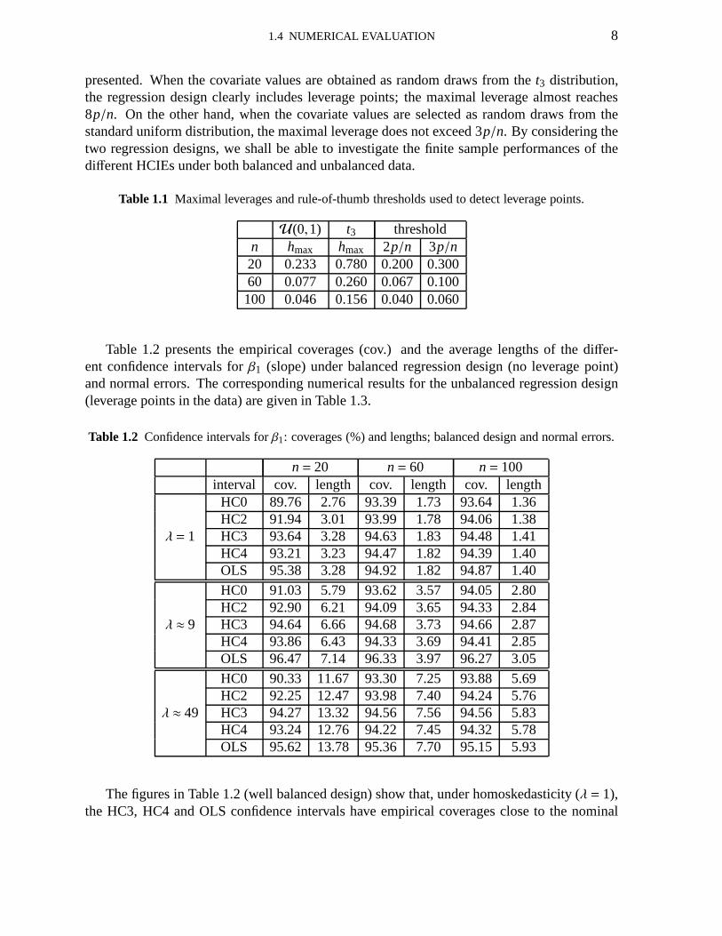
Table 1.2 presents the empirical coverages (cov.) and the average lengths of the differ-ent confidence intervals forβ1 (slope) under balanced regression design (no leverage point)and normal errors. The corresponding numerical results forthe unbalanced regression design(leverage points in the data) are given in Table 1.3.
Table 1.2 Confidence intervals forβ1: coverages (%) and lengths; balanced design and normal errors.
n= 20 n= 60 n= 100interval cov. length cov. length cov. length
HC0 89.76 2.76 93.39 1.73 93.64 1.36HC2 91.94 3.01 93.99 1.78 94.06 1.38
λ = 1 HC3 93.64 3.28 94.63 1.83 94.48 1.41HC4 93.21 3.23 94.47 1.82 94.39 1.40OLS 95.38 3.28 94.92 1.82 94.87 1.40
HC0 91.03 5.79 93.62 3.57 94.05 2.80HC2 92.90 6.21 94.09 3.65 94.33 2.84
λ ≈ 9 HC3 94.64 6.66 94.68 3.73 94.66 2.87HC4 93.86 6.43 94.33 3.69 94.41 2.85OLS 96.47 7.14 96.33 3.97 96.27 3.05
HC0 90.33 11.67 93.30 7.25 93.88 5.69HC2 92.25 12.47 93.98 7.40 94.24 5.76
λ ≈ 49 HC3 94.27 13.32 94.56 7.56 94.56 5.83HC4 93.24 12.76 94.22 7.45 94.32 5.78OLS 95.62 13.78 95.36 7.70 95.15 5.93
The figures in Table 1.2 (well balanced design) show that, under homoskedasticity (λ = 1),the HC3, HC4 and OLS confidence intervals have empirical coverages close to the nominal
1.4 NUMERICAL EVALUATION 9
level (95%) for all sample sizes. The HC0 and HC2 intervals display good coverage whenthe sample size is not small. Additionally, the average lengths of the HC3, HC4 and OLSconfidence intervals are similar. Whenλ = 9.432, the HC3 e HC4 confidence intervals displaycoverages that are close to the nominal coverage (95%) for all sample sizes. Again, the HC0and HC2 confidence intervals do not display good coverage when the sample size is small(n = 20). For instance, the empirical coverages of the HC3 and HC4confidence intervalsfor β1 whenn = 20 are, respectively, 94.64% and 93.86%, whereas the corresponding figuresfor the HC0 and HC2 confidence intervals are 91.03% and 92.90%. The average lengths ofall intervals increase substantially relative to the homoskedastic case. Whenλ = 49.126, theempirical coverages of the HC3 and HC4 confidence intervals for β1 are close to the selectednominal level for all samples sizes. Once again, the averagelengths of all intervals increasedrelative to the previous case.
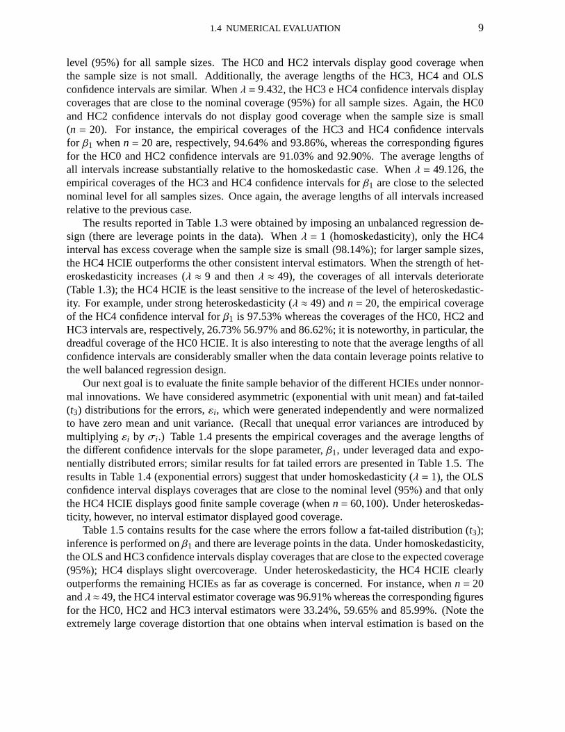
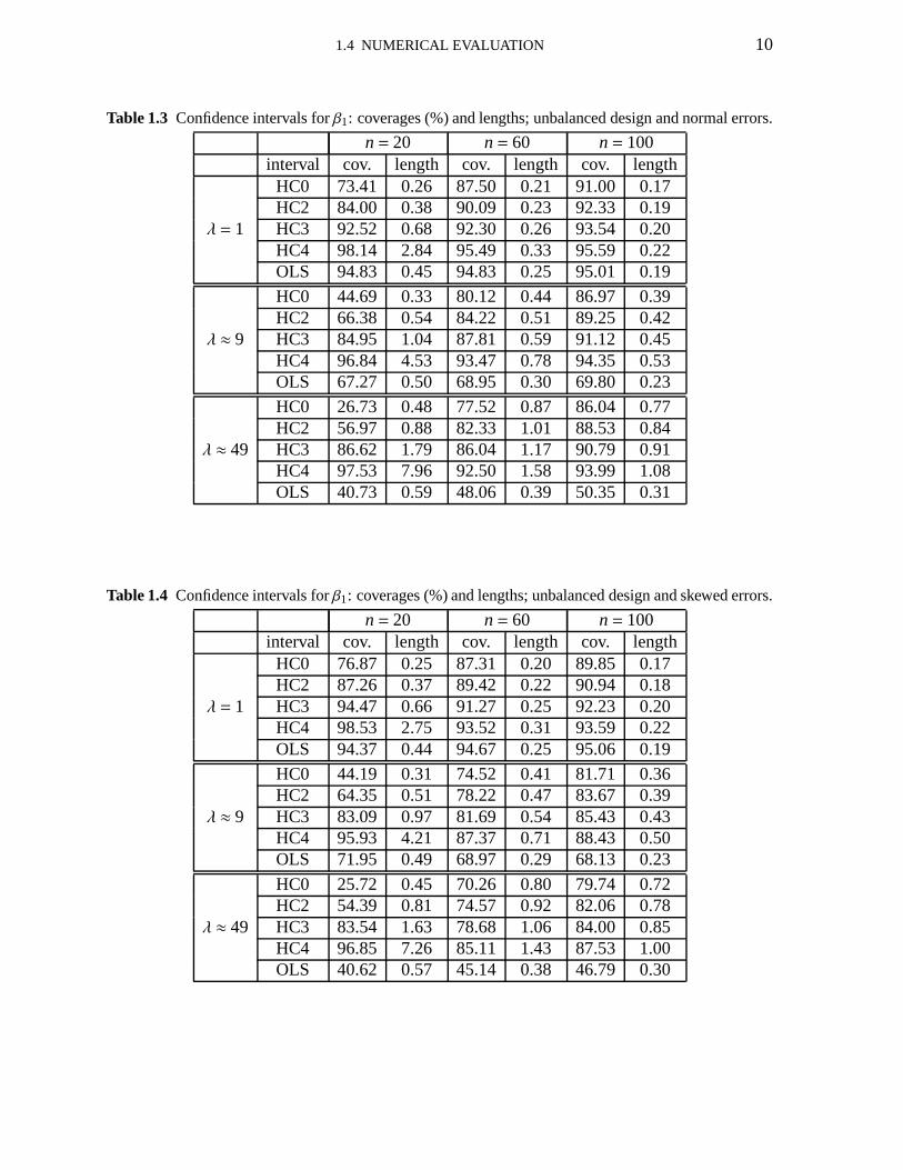
The results reported in Table 1.3 were obtained by imposing an unbalanced regression de-sign (there are leverage points in the data). Whenλ = 1 (homoskedasticity), only the HC4interval has excess coverage when the sample size is small (98.14%); for larger sample sizes,the HC4 HCIE outperforms the other consistent interval estimators. When the strength of het-eroskedasticity increases (λ ≈ 9 and thenλ ≈ 49), the coverages of all intervals deteriorate(Table 1.3); the HC4 HCIE is the least sensitive to the increase of the level of heteroskedastic-ity. For example, under strong heteroskedasticity (λ ≈ 49) andn= 20, the empirical coverageof the HC4 confidence interval forβ1 is 97.53% whereas the coverages of the HC0, HC2 andHC3 intervals are, respectively, 26.73% 56.97% and 86.62%;it is noteworthy, in particular, thedreadful coverage of the HC0 HCIE. It is also interesting to note that the average lengths of allconfidence intervals are considerably smaller when the datacontain leverage points relative tothe well balanced regression design.
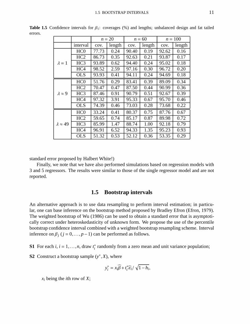
Our next goal is to evaluate the finite sample behavior of the different HCIEs under nonnor-mal innovations. We have considered asymmetric (exponential with unit mean) and fat-tailed(t3) distributions for the errors,εi , which were generated independently and were normalizedto have zero mean and unit variance. (Recall that unequal error variances are introduced bymultiplying εi by σi .) Table 1.4 presents the empirical coverages and the average lengths ofthe different confidence intervals for the slope parameter,β1, under leveraged data and expo-nentially distributed errors; similar results for fat tailed errors are presented in Table 1.5. Theresults in Table 1.4 (exponential errors) suggest that under homoskedasticity (λ = 1), the OLSconfidence interval displays coverages that are close to thenominal level (95%) and that onlythe HC4 HCIE displays good finite sample coverage (whenn= 60,100). Under heteroskedas-ticity, however, no interval estimator displayed good coverage.
Table 1.5 contains results for the case where the errors follow a fat-tailed distribution (t3);inference is performed onβ1 and there are leverage points in the data. Under homoskedasticity,the OLS and HC3 confidence intervals display coverages that are close to the expected coverage(95%); HC4 displays slight overcoverage. Under heteroskedasticity, the HC4 HCIE clearlyoutperforms the remaining HCIEs as far as coverage is concerned. For instance, whenn= 20andλ≈ 49, the HC4 interval estimator coverage was 96.91% whereas the corresponding figuresfor the HC0, HC2 and HC3 interval estimators were 33.24%, 59.65% and 85.99%. (Note theextremely large coverage distortion that one obtains when interval estimation is based on the
1.4 NUMERICAL EVALUATION 10
Table 1.3 Confidence intervals forβ1: coverages (%) and lengths; unbalanced design and normal errors.
n= 20 n= 60 n= 100interval cov. length cov. length cov. length
HC0 73.41 0.26 87.50 0.21 91.00 0.17HC2 84.00 0.38 90.09 0.23 92.33 0.19
λ = 1 HC3 92.52 0.68 92.30 0.26 93.54 0.20HC4 98.14 2.84 95.49 0.33 95.59 0.22OLS 94.83 0.45 94.83 0.25 95.01 0.19
HC0 44.69 0.33 80.12 0.44 86.97 0.39HC2 66.38 0.54 84.22 0.51 89.25 0.42
λ ≈ 9 HC3 84.95 1.04 87.81 0.59 91.12 0.45HC4 96.84 4.53 93.47 0.78 94.35 0.53OLS 67.27 0.50 68.95 0.30 69.80 0.23
HC0 26.73 0.48 77.52 0.87 86.04 0.77HC2 56.97 0.88 82.33 1.01 88.53 0.84
λ ≈ 49 HC3 86.62 1.79 86.04 1.17 90.79 0.91HC4 97.53 7.96 92.50 1.58 93.99 1.08OLS 40.73 0.59 48.06 0.39 50.35 0.31
Table 1.4 Confidence intervals forβ1: coverages (%) and lengths; unbalanced design and skewed errors.
n= 20 n= 60 n= 100interval cov. length cov. length cov. length
HC0 76.87 0.25 87.31 0.20 89.85 0.17HC2 87.26 0.37 89.42 0.22 90.94 0.18
λ = 1 HC3 94.47 0.66 91.27 0.25 92.23 0.20HC4 98.53 2.75 93.52 0.31 93.59 0.22OLS 94.37 0.44 94.67 0.25 95.06 0.19
HC0 44.19 0.31 74.52 0.41 81.71 0.36HC2 64.35 0.51 78.22 0.47 83.67 0.39
λ ≈ 9 HC3 83.09 0.97 81.69 0.54 85.43 0.43HC4 95.93 4.21 87.37 0.71 88.43 0.50OLS 71.95 0.49 68.97 0.29 68.13 0.23
HC0 25.72 0.45 70.26 0.80 79.74 0.72HC2 54.39 0.81 74.57 0.92 82.06 0.78
λ ≈ 49 HC3 83.54 1.63 78.68 1.06 84.00 0.85HC4 96.85 7.26 85.11 1.43 87.53 1.00OLS 40.62 0.57 45.14 0.38 46.79 0.30
1.5 BOOTSTRAP INTERVALS 11
Table 1.5 Confidence intervals forβ1: coverages (%) and lengths; unbalanced design and fat tailederrors.
n= 20 n= 60 n= 100interval cov. length cov. length cov. length
HC0 77.73 0.24 90.40 0.19 92.62 0.16HC2 86.73 0.35 92.63 0.21 93.87 0.17
λ = 1 HC3 93.89 0.62 94.40 0.24 95.02 0.18HC4 98.52 2.59 97.16 0.30 96.72 0.20OLS 93.93 0.41 94.11 0.24 94.69 0.18
HC0 51.76 0.29 83.41 0.39 89.09 0.34HC2 70.47 0.47 87.50 0.44 90.99 0.36
λ ≈ 9 HC3 87.46 0.91 90.79 0.51 92.67 0.39HC4 97.32 3.91 95.33 0.67 95.70 0.46OLS 74.39 0.46 73.03 0.28 73.68 0.22
HC0 33.24 0.41 80.37 0.75 87.76 0.67HC2 59.65 0.74 85.17 0.87 89.98 0.72
λ ≈ 49 HC3 85.99 1.47 88.74 1.00 92.18 0.79HC4 96.91 6.52 94.33 1.35 95.23 0.93OLS 51.32 0.53 52.12 0.36 53.35 0.29
standard error proposed by Halbert White!)Finally, we note that we have also performed simulations based on regression models with
3 and 5 regressors. The results were similar to those of the single regressor model and are notreported.
1.5 Bootstrap intervals
An alternative approach is to use data resampling to performinterval estimation; in particu-lar, one can base inference on the bootstrap method proposedby Bradley Efron (Efron, 1979).The weighted bootstrap of Wu (1986) can be used to obtain a standard error that is asymptoti-cally correct under heteroskedasticity of unknown form. Wepropose the use of the percentilebootstrap confidence interval combined with a weighted bootstrap resampling scheme. Intervalinference onβ j ( j = 0, . . . , p−1) can be performed as follows.
S1 For eachi, i = 1, . . . ,n, drawt∗i randomly from a zero mean and unit variance population;
S2 Construct a bootstrap sample (y∗,X), where
y∗i = xi β+ t∗i εi/√
1−hi ,
xi being theith row of X;
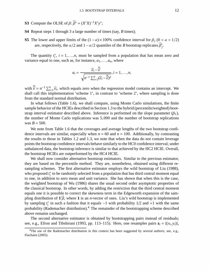
1.5 BOOTSTRAP INTERVALS 12
S3 Compute the OLSE ofβ: β∗ = (X′X)−1X′y∗;
S4 Repeat steps 1 through 3 a large number of times (say,B times);
S5 The lower and upper limits of the (1−α)×100% confidence interval forβ j (0 < α < 1/2)are, respectively, theα/2 and 1−α/2 quantiles of theB bootstrap replicatesβ∗j .
The quantityt∗i , i = 1, . . . ,n, must be sampled from a population that has mean zero andvariance equal to one, such as, for instance,a1, . . . ,an, where
ai =εi − ε√
n−1∑ni=1(εi − ε)2
, i = 1, . . . ,n,
with ε = n−1∑ni=1 εi , which equals zero when the regression model contains an intercept. We
shall call this implementation ‘scheme 1’, in contrast to ‘scheme 2’, where sampling is donefrom the standard normal distribution.
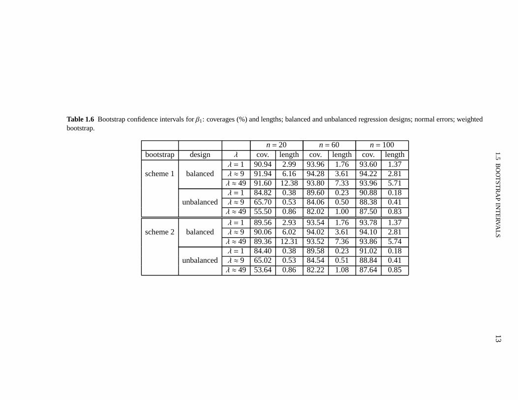
In what follows (Table 1.6), we shall compare, using Monte Carlo simulations, the finitesample behavior of the HCIEs described in Section 1.3 to the hybrid (percentile/weighted) boot-strap interval estimator described above. Inference is performed on the slope parameter (β1),the number of Monte Carlo replications was 5,000 and the number of bootstrap replicationswasB= 500.
We note from Table 1.6 that the coverages and average lengthsof the two bootstrap confi-dence intervals are similar, especially whenn= 60 andn = 100. Additionally, by contrastingthe results to those in Tables 1.2 and 1.3, we note that when the data do not contain leveragepoints the bootstrap confidence intervals behave similarlyto the HC0 confidence interval; underunbalanced data, the bootstrap inference is similar to thatachieved by the HC2 HCIE. Overall,the bootstrap HCIEs are outperformed by the HC4 HCIE.
We shall now consider alternative bootstrap estimators. Similar to the previous estimator,they are based on the percentile method. They are, nonetheless, obtained using different re-sampling schemes. The first alternative estimator employs the wild bootstrap of Liu (1988),who proposedt∗i to be randomly selected from a population that has third central moment equalto one, in addition to zero mean and unit variance. She has shown that when this is the case,the weighted bootstrap of Wu (1986) shares the usual second order asymptotic properties ofthe classical bootstrap. In other words, by adding the restriction that the third central momentequals one it is possible to correct the skewness term in the Edgeworth expansion of the sam-pling distribution of1′β, where1 is ann-vector of ones. Liu’s wild bootstrap is implementedby samplingt∗i in such a fashion that it equals−1 with probability 1/2 and+1 with the sameprobability (Rademacher distribution).4 The remainder of the bootstrapping scheme describedabove remains unchanged.
The second alternative estimator is obtained by bootstrapping pairs instead of residuals;see, e.g., Efron and Tibshirani (1993, pp. 113–115). Here, one resamples pairszi = (xi ,yi),
4The use of the Rademacher distribution in this context has been suggested by several authors; see, e.g.,Flachaire (2005).
1.5
BO
OT
ST
RA
PIN
TE
RVA
LS
13
Table 1.6 Bootstrap confidence intervals forβ1: coverages (%) and lengths; balanced and unbalanced regression designs; normal errors; weightedbootstrap.
n= 20 n= 60 n= 100bootstrap design λ cov. length cov. length cov. length
λ = 1 90.94 2.99 93.96 1.76 93.60 1.37scheme 1 balanced λ ≈ 9 91.94 6.16 94.28 3.61 94.22 2.81
λ ≈ 49 91.60 12.38 93.80 7.33 93.96 5.71λ = 1 84.82 0.38 89.60 0.23 90.88 0.18
unbalanced λ ≈ 9 65.70 0.53 84.06 0.50 88.38 0.41λ ≈ 49 55.50 0.86 82.02 1.00 87.50 0.83
λ = 1 89.56 2.93 93.54 1.76 93.78 1.37scheme 2 balanced λ ≈ 9 90.06 6.02 94.02 3.61 94.10 2.81
λ ≈ 49 89.36 12.31 93.52 7.36 93.86 5.74λ = 1 84.40 0.38 89.58 0.23 91.02 0.18
unbalanced λ ≈ 9 65.02 0.53 84.54 0.51 88.84 0.41λ ≈ 49 53.64 0.86 82.22 1.08 87.64 0.85
1.5 BOOTSTRAP INTERVALS 14
i = 1, . . . ,n. The parameter vectorβ is estimated using the bootstrap sample of responsesy∗ = (y∗1, . . . ,y
∗n)′ together with the pseudo-design matrixX∗ formed out ofx∗1, . . . , x
∗n. This boot-
strapping scheme is also known as the (y,X) bootstrap.The simulation results for interval inference onβ1 using the two alternative bootstrap in-
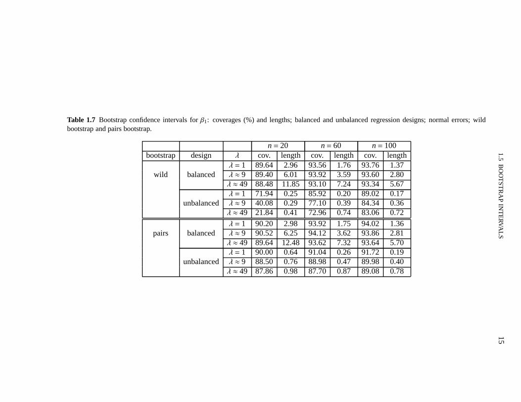
terval estimators described above, i.e., the estimators based on the wild bootstrap and on thebootstrap of pairs of observations, are presented in Table 1.7. The number of Monte Carloand bootstrap replications are as before. The figures in Table 1.7, when contrasted with thesimulation results reported in Table 1.6, show that the weighted bootstrap estimator slightlyoutperforms the wild bootstrap estimator when the regression design is balanced but under un-balanced regression designs it is clearly better. Indeed, when the sample size is small (n= 20)and heteroskedasticity is strong, the coverage of the wild bootstrap estimator can be dreadful(e.g., 21.84% when the desired coverage is 95%;λ≈ 49). The figures in Table 1.7 also show thatthe estimator obtained by bootstrapping pairs of observations outperforms both the weightedand wild bootstrap estimators when the regressors matrix contains leverage points. For instan-ce, whenn= 20,λ ≈ 49 and there are observations with high leverage in the data,the empiricalcoverages of the weighted (scheme 1) and wild bootstrap interval estimators are 55.50% and21.84%, respectively, whereas the empirical coverage of the interval bootstrap estimator thatuses bootstrapping of pairs is 87.86%.
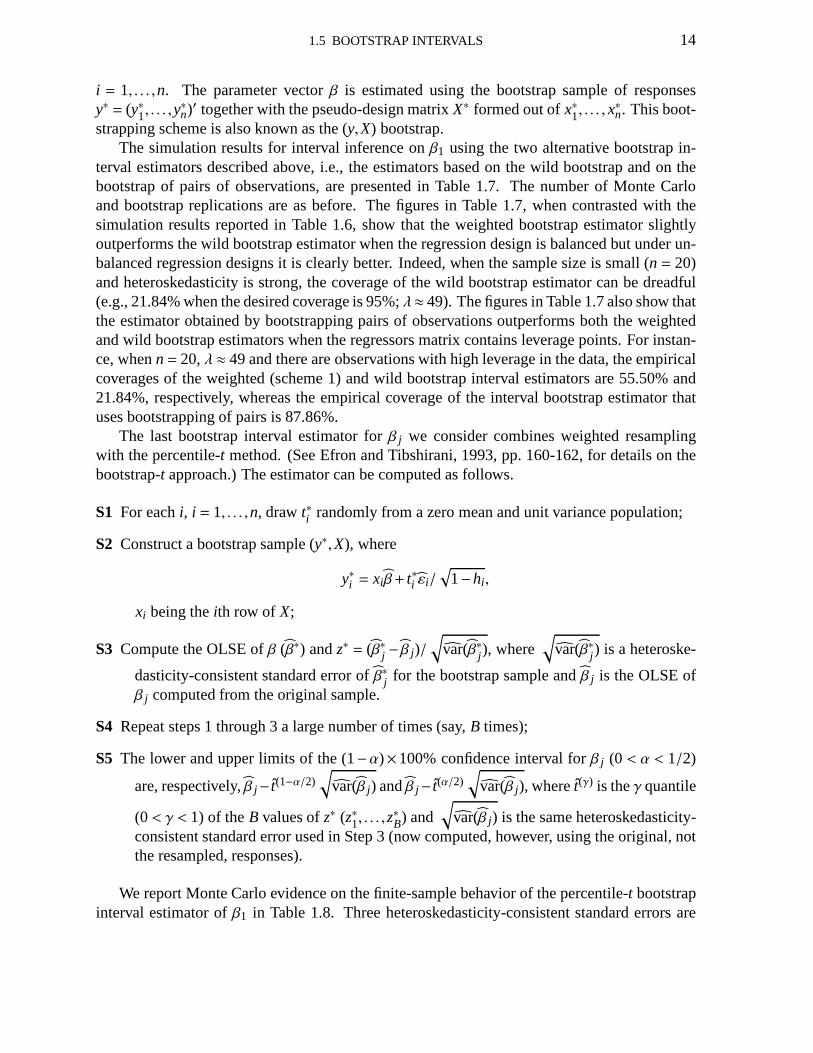
The last bootstrap interval estimator forβ j we consider combines weighted resamplingwith the percentile-t method. (See Efron and Tibshirani, 1993, pp. 160-162, for details on thebootstrap-t approach.) The estimator can be computed as follows.
S1 For eachi, i = 1, . . . ,n, drawt∗i randomly from a zero mean and unit variance population;
S2 Construct a bootstrap sample (y∗,X), where
y∗i = xi β+ t∗i εi/√
1−hi ,
xi being theith row of X;
S3 Compute the OLSE ofβ (β∗) andz∗ = (β∗j − β j)/√
var(β∗j ), where√
var(β∗j ) is a heteroske-
dasticity-consistent standard error ofβ∗j for the bootstrap sample andβ j is the OLSE ofβ j computed from the original sample.
S4 Repeat steps 1 through 3 a large number of times (say,B times);
S5 The lower and upper limits of the (1−α)×100% confidence interval forβ j (0 < α < 1/2)
are, respectively,β j− t(1−α/2)√
var(β j) andβ j− t(α/2)√
var(β j), wheret(γ) is theγ quantile
(0< γ < 1) of theB values ofz∗ (z∗1, . . . ,z∗B) and
√var(β j) is the same heteroskedasticity-
consistent standard error used in Step 3 (now computed, however, using the original, notthe resampled, responses).
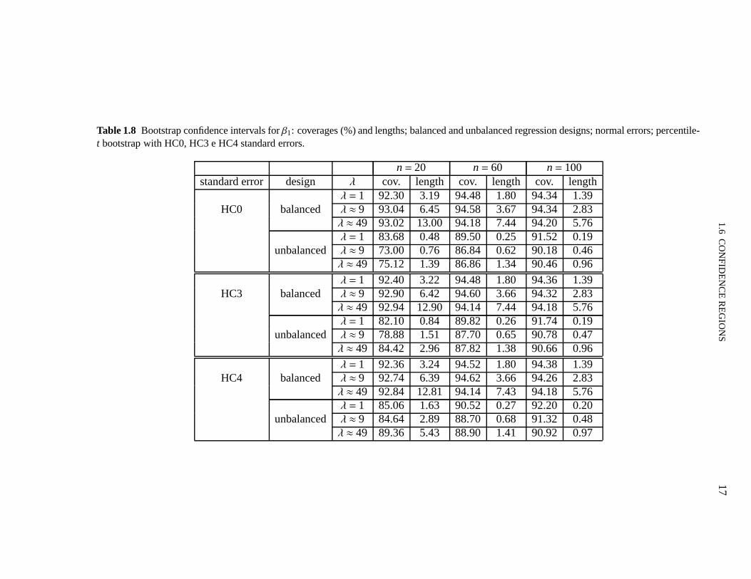
We report Monte Carlo evidence on the finite-sample behaviorof the percentile-t bootstrapinterval estimator ofβ1 in Table 1.8. Three heteroskedasticity-consistent standard errors are
1.5
BO
OT
ST
RA
PIN
TE
RVA
LS
15
Table 1.7 Bootstrap confidence intervals forβ1: coverages (%) and lengths; balanced and unbalanced regression designs; normal errors; wildbootstrap and pairs bootstrap.
n= 20 n= 60 n= 100bootstrap design λ cov. length cov. length cov. length
λ = 1 89.64 2.96 93.56 1.76 93.76 1.37wild balanced λ ≈ 9 89.40 6.01 93.92 3.59 93.60 2.80
λ ≈ 49 88.48 11.85 93.10 7.24 93.34 5.67λ = 1 71.94 0.25 85.92 0.20 89.02 0.17
unbalanced λ ≈ 9 40.08 0.29 77.10 0.39 84.34 0.36λ ≈ 49 21.84 0.41 72.96 0.74 83.06 0.72
λ = 1 90.20 2.98 93.92 1.75 94.02 1.36pairs balanced λ ≈ 9 90.52 6.25 94.12 3.62 93.86 2.81
λ ≈ 49 89.64 12.48 93.62 7.32 93.64 5.70λ = 1 90.00 0.64 91.04 0.26 91.72 0.19
unbalanced λ ≈ 9 88.50 0.76 88.98 0.47 89.98 0.40λ ≈ 49 87.86 0.98 87.70 0.87 89.08 0.78
1.6 CONFIDENCE REGIONS 16
used in Steps 3 and 5, namely: HC0, HC3 and HC4.t∗i , i = 1, . . . ,n, has been sampled fromthe standard normal distribution, and, as before, 1−α = 0.95. The results show that whenthe data are not leveraged it does not make much difference which consistent standard error isused in the bootstrapping scheme. However, in unbalanced situations the percentile-t bootstrapwith HC4 standard errors displays superior behavior, especially when the sample size is small.For example, whenn= 20 and under strong heteroskedasticity, the coverages of the bootstrap-tconfidence intervals with HC0, HC3 and HC4 standard errors are 75.12%, 84.42% and 89.36%,respectively.
Overall, the best performing bootstrap estimator is the (y,X) bootstrap estimator when thesample size is small (n = 20) and the percentile-t bootstrap estimator when the sample size islarge (n= 100). It is noteworthy, however, that the HC4 HCCIE outperforms all bootstrap-basedinterval estimators.
1.6 Confidence regions
We shall now consider confidence regions that are asymptotically valid under heteroskedasticityof unknown form. To that end, we write the regression model
y= Xβ+ε
asy= X1β1+X2β2+ε, (1.6.1)
wherey, X, β andε are as described in Section 1.2,X j andβ j aren× p j andp j ×1, respectively,j = 1,2, with p= p1+ p2 such thatX = [X1 X2] andβ = (β′1,β
′2)′.
The OLSE of the vector of regression coefficients in (1.6.1) isβ =(β′1, β
′2)′, where
β2 =(R′2R2
)−1R′2y,
with R2 = M1X2 andM1 = In−X1(X′1X1)−1X′1. Sinceβ2 is asymptotically normal with meanvectorβ2 and covariance matrix
V22=(R′2R2
)−1R′2ΩR2
(R′2R2
)−1,
the quadratic formW=
(β2−β2
)′V−1
22
(β2−β2
)
is asymptoticallyχ2p2
; the result still holds whenV22 is replaced by a function of the dataV22
such that plim(V22
)= V22. In particular, we can use the following consistent estimator of the
covariance matrix ofβ2:V(k)
22 = (R′2R2)−1R′2ΩkR2(R′2R2)−1,
whereΩk, k= 0,2,3,4, is as defined in Section 1.2.
1.6
CO
NF
IDE
NC
ER
EG
ION
S1
7
Table 1.8 Bootstrap confidence intervals forβ1: coverages (%) and lengths; balanced and unbalanced regression designs; normal errors; percentile-t bootstrap with HC0, HC3 e HC4 standard errors.
n= 20 n= 60 n= 100standard error design λ cov. length cov. length cov. length
λ = 1 92.30 3.19 94.48 1.80 94.34 1.39HC0 balanced λ ≈ 9 93.04 6.45 94.58 3.67 94.34 2.83
λ ≈ 49 93.02 13.00 94.18 7.44 94.20 5.76λ = 1 83.68 0.48 89.50 0.25 91.52 0.19
unbalanced λ ≈ 9 73.00 0.76 86.84 0.62 90.18 0.46λ ≈ 49 75.12 1.39 86.86 1.34 90.46 0.96
λ = 1 92.40 3.22 94.48 1.80 94.36 1.39HC3 balanced λ ≈ 9 92.90 6.42 94.60 3.66 94.32 2.83
λ ≈ 49 92.94 12.90 94.14 7.44 94.18 5.76λ = 1 82.10 0.84 89.82 0.26 91.74 0.19
unbalanced λ ≈ 9 78.88 1.51 87.70 0.65 90.78 0.47λ ≈ 49 84.42 2.96 87.82 1.38 90.66 0.96
λ = 1 92.36 3.24 94.52 1.80 94.38 1.39HC4 balanced λ ≈ 9 92.74 6.39 94.62 3.66 94.26 2.83
λ ≈ 49 92.84 12.81 94.14 7.43 94.18 5.76λ = 1 85.06 1.63 90.52 0.27 92.20 0.20
unbalanced λ ≈ 9 84.64 2.89 88.70 0.68 91.32 0.48λ ≈ 49 89.36 5.43 88.90 1.41 90.92 0.97

1.6 CONFIDENCE REGIONS 18
Let 0< α < 1 and letχ2p2,α
be such that
Pr(χ2p2< χ2
p2,α) = 1−α;
that is,χ2p2,α
is the 1−α upper quantile of theχ2p2
distribution. Also, let
W(k) =(β2−β2
)′ (V(k)
22
)−1 (β2−β2
).
Thus, the 100(1−α)% confidence region forβ2 is given by the set of values ofβ2 such that
W(k) < χ2p2,α. (1.6.2)
In what follows we shall numerically evaluate the finite sample performance of the differentconfidence regions. The regression model used in the simulation is
yi = β0+β1xi1+β2xi2+εi , i = 1, . . . ,n,
whereεi is a zero mean normally distributed error which is free of serial correlation.The covariate values were, as before, selected as random draws from the standard uniform
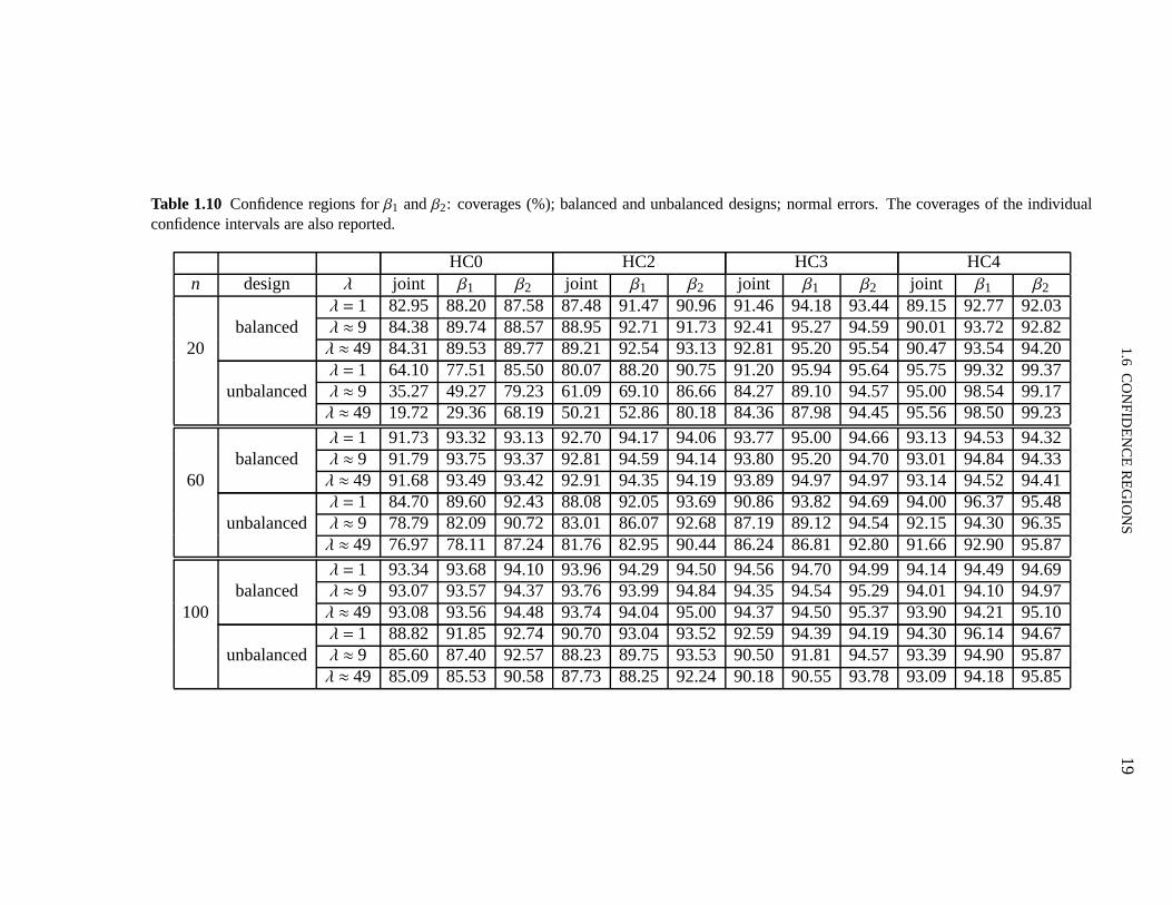
(well balanced design) andt3 (unbalanced) distributions. The number of Monte Carlo replica-tions was 10,000, the sample sizes considered weren= 20,60,100 and 1−α= 0.95; simulationswere performed under both homoskedasticity and heteroskedasticity. The reported coveragescorrespond to the percentage of replications in which (1.6.2) holds when inference is performedonβ1 andβ2 (jointly). In order to contrast the finite sample performances of confidence regions(‘joint’) and confidence intervals (forβ1 andβ2 separately), individual coverages are also re-ported.
Table 1.9 contains the maximal leverages of the two regression designs together with theusual thresholds used in the detection of leverage points. We note that the design in which thecovariate values were selected as draws from a Studentt distribution includes observations withvery high leverage, unlike the other design (standard uniform draws).
Table 1.9 Maximal leverages and rule-of-thumb thresholds used to detect leverage points; two covari-ates
U(0,1) t3 thresholdn hmax hmax 2p/n 3p/n20 0.261 0.858 0.30 0.4560 0.087 0.286 0.10 0.15100 0.052 0.172 0.06 0.09
Table 1.10 contains the coverages of the different confidence regions (‘joint’) and also of theindividual confidence intervals for 1−α = 0.95. We note, at the outset, that the joint coveragesare always smaller than the individual ones, the difference being larger when the regression
1.6
CO
NF
IDE
NC
ER
EG
ION
S1
9
Table 1.10 Confidence regions forβ1 andβ2: coverages (%); balanced and unbalanced designs; normal errors. The coverages of the individualconfidence intervals are also reported.
HC0 HC2 HC3 HC4n design λ joint β1 β2 joint β1 β2 joint β1 β2 joint β1 β2
λ = 1 82.95 88.20 87.58 87.48 91.47 90.96 91.46 94.18 93.44 89.15 92.77 92.03balanced λ ≈ 9 84.38 89.74 88.57 88.95 92.71 91.73 92.41 95.27 94.59 90.01 93.72 92.82
20 λ ≈ 49 84.31 89.53 89.77 89.21 92.54 93.13 92.81 95.20 95.54 90.47 93.54 94.20λ = 1 64.10 77.51 85.50 80.07 88.20 90.75 91.20 95.94 95.64 95.75 99.32 99.37
unbalanced λ ≈ 9 35.27 49.27 79.23 61.09 69.10 86.66 84.27 89.10 94.57 95.00 98.54 99.17λ ≈ 49 19.72 29.36 68.19 50.21 52.86 80.18 84.36 87.98 94.45 95.56 98.50 99.23
λ = 1 91.73 93.32 93.13 92.70 94.17 94.06 93.77 95.00 94.66 93.13 94.53 94.32balanced λ ≈ 9 91.79 93.75 93.37 92.81 94.59 94.14 93.80 95.20 94.70 93.01 94.84 94.33
60 λ ≈ 49 91.68 93.49 93.42 92.91 94.35 94.19 93.89 94.97 94.97 93.14 94.52 94.41λ = 1 84.70 89.60 92.43 88.08 92.05 93.69 90.86 93.82 94.69 94.00 96.37 95.48
unbalanced λ ≈ 9 78.79 82.09 90.72 83.01 86.07 92.68 87.19 89.12 94.54 92.15 94.30 96.35λ ≈ 49 76.97 78.11 87.24 81.76 82.95 90.44 86.24 86.81 92.80 91.66 92.90 95.87
λ = 1 93.34 93.68 94.10 93.96 94.29 94.50 94.56 94.70 94.99 94.14 94.49 94.69balanced λ ≈ 9 93.07 93.57 94.37 93.76 93.99 94.84 94.35 94.54 95.29 94.01 94.10 94.97
100 λ ≈ 49 93.08 93.56 94.48 93.74 94.04 95.00 94.37 94.50 95.37 93.90 94.21 95.10λ = 1 88.82 91.85 92.74 90.70 93.04 93.52 92.59 94.39 94.19 94.30 96.14 94.67
unbalanced λ ≈ 9 85.60 87.40 92.57 88.23 89.75 93.53 90.50 91.81 94.57 93.39 94.90 95.87λ ≈ 49 85.09 85.53 90.58 87.73 88.25 92.24 90.18 90.55 93.78 93.09 94.18 95.85
1.7 CONCLUDING REMARKS 20
design is unbalanced. It can also be seen that whenn = 20 the HC0 and HC2 regions andintervals can display severe undercoverage. For instance,the HC0 (HC2) confidence regioncoverage whenn= 20, the data includes observations with high leverage and heteroskedastic-ity is strong is less than 20% (approximately 50%), which is much smaller than the nominalcoverage (95%); the corresponding HC3 and HC4 confidence regions coverages, in contrast,are 84.36% and 95.56%. Overall, the results show that the HC4confidence region outperformsthe competition, especially under leveraged data. The HC3 confidence region is competitivewhen the regression design is well balanced.
1.7 Concluding remarks
It is oftentimes desirable to perform asymptotically correct inference on the parameters that in-dex the linear regression model under heteroskedasticity of unknown form. Different varianceand covariance estimators have been proposed in the literature, and numerical evidence on thefinite sample performance of these point estimators and associated hypothesis tests are avail-able. In this chapter, we have considered and numerically evaluated the finite sample behaviorof a class of heteroskedasicity-consistent interval/region estimators. The numerical evaluationwas carried out under both homoskedasticity and heteroskedasticity; regression designs bothwithout and with high leverage observations were considered. The results show that intervalestimation based on the popular White (HC0) estimator can bequite misleading when the sam-ple size is not large. Overall, the results favor the HC4 interval estimator, which displayedmuch more reliable finite sample behavior than the HC0 and HC2interval estimators, and evenoutperformed its HC3 counterpart.
Bootstrap interval estimation was also considered. Four bootstrap interval estimators weredescribed and evaluated, namely: weighted, wild, pairs andpercentile-t. The best performingbootstrap estimators were the pairs bootstrap estimator and that obtained using the percentile-tmethod, the former displaying superior behavior when the sample size was small and the latterbeing superior for larger sample sizes (100 observations, in the case of our numerical exercise).It is also noteworthy that the wild bootstrap interval estimator displayed poor coverage underleveraged data, its exact coverage being over four times smaller than the desired coverage in anextreme situation (small sample size, strong heteroskedasticity, leveraged data).
Based on the results in this chapter, we encourage practitioners to perform interval inferencein linear regressions using the HC4 interval estimator.
C 2
Bias-adjusted covariance matrix estimators
2.1 Introduction
Homoskedasticity is a commonly violated assumption in the linear regression model. It statesthat the error variances are constant across all observations, regardless of the covariate values.The ordinary least squares estimator (OLSE) of the vector ofregression parameters remainsunbiased, consistent and asymptotically normal even when such an assumption does not hold.The OLSE is thus a valid estimator even under heteroskedasticity of unknown form. In orderto perform asymptotically valid interval estimation and hypothesis testing inference, however,one needs to obtain a consistent estimator of the OLSE covariance matrix which can yield, forinstance, asymptotically valid standard errors. White (1980), in an influential paper, showedthat consistent standard errors can be easily obtained using a sandwich-type estimator. Hisestimator, which we shall call HC0, is considerably biased in finite samples; in particular, ittends to be quite optimistic, i.e., it underestimates the true variances, especially when the datacontain leverage points. A more accurate estimator was proposed by Qian and Wang (2001).Their estimator usually displays much smaller biases in samples of small to moderate sizes. Ourchief goal in this chapter is twofold. First, we improve upontheir estimator by bias correctingit in an iterative fashion. To that end, we derive a sequence of bias adjusted estimators suchthat the orders of the respective biases decrease as we move along the sequence. Our numericalresults show that the proposed bias correcting scheme can bequite effective in some situations.Second, we define a class of heteroskedasticity-consistentcovariance matrix estimators whichincludes modified versions of some well known variants of White’s estimator, and argue thatthe results obtained for the Qian–Wang estimator can be easily extended to this new class ofestimators.
A few remarks are in order. First, bias correction may inducevariance inflation, as notedby MacKinnon and Smith (1998). Indeed, our numerical results indicate that this is the case.Second, it is also possible to achieve increasing precisionas far as bias is concerned by using theiterated bootstrap, which is, nonetheless, highly computer intensive. Our sequence of modifiedestimators achieves similar precision with almost no computational burden. For details onthe relation between the two approaches (analytical and bootstrap) to iterated corrections, seeFerrari and Cribari–Neto (1998). Third, finite sample corrections to White’s estimator wereobtained by Cribari–Neto, Ferrari and Cordeiro (2000). Ourresults, however, apply to anestimator proposed by Qian and Wang (2001) which is more accurate than White’s estimator;it is even unbiased under equal error variances. Additionally, we show that the Qian–Wangestimator can be generalized into a class that includes modified versions of well known variantsof White’s estimator, and argue that the results obtained for the Qian–Wang estimator can be
21

2.2 THE MODEL AND COVARIANCE MATRIX ESTIMATORS 22
generalized to this broader class of heteroskedasticity-robust estimators.The chapter unfolds as follows. Section 2.2 introduces the linear regression model and some
heteroskedasticity-consistent covariance matrix estimators. In Section 2.3 we derive a sequenceof consistent estimators for the covariance matrix of the ordinary least squares estimator. Wedo so by defining a sequential bias correcting scheme which isinitialized at the estimator pro-posed by Qian and Wang (2001). In Section 2.4 we obtain estimators for the variance of linearcombinations of the elements in the vector of ordinary leastsquares estimators. Results froma numerical evaluation are presented in Section 2.5; these are exact, not Monte Carlo results.Two empirical applications that use real data are presentedand discussed in Section 2.6. In Sec-tion 2.7 we show that modified versions of variants of HalbertWhite’s estimator can be easilyobtained, and that the resulting estimators can be easily adjusted for bias; as a consequence, allof the results we derive can be extended to cover estimators other than that proposed by Qianand Wang (2001). Finally, Section 2.8 offers some concluding remarks.
2.2 The model and covariance matrix estimators
The model of interest is the linear regression model, which can be written as
y= Xβ+ε,
wherey andε aren×1 vectors of responses and errors, respectively,X is a full column rankfixedn× p matrix of regressors (rank(X) = p< n) andβ = (β1, . . . ,βp)′ is ap-vector of unknownregression parameters. The errorεi has mean zero, variance 0< σ2
i < ∞, i = 1, . . . ,n, andis uncorrelated toε j wheneverj , i. Let Ω denote the covariance matrix of the errors, i.e.,Ω = cov(ε) = diagσ2
i .The OLSE ofβ can be written in closed-form asβ = (X′X)−1X′y. It is unbiased, consistent
and asymptotically normal even under unequal error variances. Its covariance matrix isΨ =cov(β) = PΩP′, whereP = (X′X)−1X′. Under homoskedasticity,σ2
i = σ2, i = 1, . . . ,n, where
σ2 > 0, and henceΨ = σ2(X′X)−1. The covariance matrixΨ can then be easily estimated as
Ψ = σ2(X′X)−1,
whereσ2 = (y−Xβ)′(y−Xβ)/(n− p).Under heteroskedaticity, it is common practice to use the OLSE coupled with a consistent
covariance matrix estimator. To that end, one uses an estimator Ω of Ω (which isn×n) suchthatX′ΩX is consistent forX′ΩX (which is p× p), i.e., plim[(X′ΩX)−1(X′ΩX)] = Ip, whereIp
is thep-dimensional identity matrix.1
White (1980) obtained a consistent estimator forΨ. His estimator is consistent under bothhomoskedasticity and heteroskedasticity of unknown form,and can be written as
HC0= Ψ = PΩP′,
1In what follows, we shall omit the order subscript when denoting the identity matrix; the order must beimplicitly understood.
2.2 THE MODEL AND COVARIANCE MATRIX ESTIMATORS 23
whereΩ = diagε2i . Here,εi is theith least squares residual, i.e.,εi = yi − xi β, wherexi is theith row of X, i = 1, . . . ,n. The vector of least squares residuals isε = (ε1, . . . , εn)′ = (I −H)y,whereH = X(X′X)−1X′ = XP is a symmetric and idempotent matrix known as ‘the hat matrix’.The diagonal elements ofH (h1, . . . ,hn) assume values in the standard unit interval (0,1) andadd up top; thus, they averageh= p/n. These quantities are used as measures of the leveragesof the corresponding observations. A rule-of-thumb statesthat observations such thathi > 2p/nor hi > 3p/n are taken to be leverage points; see, e.g., Davidson and MacKinnon (1993).
The numerical evidence in Cribari–Neto and Zarkos (1999, 2001), Long and Ervin (2000)and MacKinnon and White (1985) showed that the estimator proposed by Halbert White can bequite biased in finite samples and that associated hypothesis tests can be quite liberal. Chesherand Jewitt (1987) showed that the negative HC0 bias is largely due to the presence of observa-tions with high leverage in the data.
Several variants of the HC0 estimator were proposed in the literature, such as
(i) (Hinkley, 1977) HC1= PΩ1P′ = PD1ΩP′, whereD1 = (n/(n− p))I ;
(ii) (Horn, Horn and Duncan, 1975) HC2= PΩ2P′ = PD2ΩP′, where
D2 = diag1/(1−hi);
(iii) (Davidson and MacKinnon, 1993) HC3= PΩ3P′ = PD3ΩP′, where
D3 = diag1/(1−hi)2;
(iv) (Cribari–Neto, 2004) HC4= PΩ4P′ = PD4ΩP′, where
D4 = diag1/(1−hi)δi , δi =min4,nhi/p.
As noted earlier, the HC0 estimator is considerably biased in samples of small to moderatesizes. Cribari–Neto, Ferrari and Cordeiro (2000) derived bias adjusted variants of HC0 by usingan iterative bias correction mechanism. The chain of estimators was obtained by correctingHC0, then correcting the resulting adjusted estimator, andso on.
Let (A)d denote the diagonal matrix obtained by setting the nondiagonal elements of thesquare matrixA equal to zero. Note thatΩ = (εε′)d. Thus,
E(εε′) = cov(ε)+E(ε)E(ε′)
= (I −H)Ω(I −H)
since (I −H)X = 0. It thus follows thatE(Ω) = (I −H)Ω(I −H)d andE(Ψ) = PE(Ω)P′. Hence,the biases ofΩ andΨ as estimators ofΩ andΨ are
BΩ
(Ω) = E(Ω)−Ω = HΩ(H −2I )d
andBΨ
(Ω) = E(Ψ)−Ψ = PBΩ
(Ω)P′,

2.2 THE MODEL AND COVARIANCE MATRIX ESTIMATORS 24
respectively.Cribari–Neto, Ferrari and Cordeiro (2000) define the bias corrected estimator
Ω(1) = Ω−BΩ
(Ω).
This estimator can be in turn bias corrected:
Ω(2) = Ω(1)−BΩ(1)(Ω),
and so on. Afterk iterations of the bias correcting scheme one obtains
Ω(k) = Ω(k−1)−BΩ(k−1)(Ω).
Consider the following recursive function of ann×n diagonal matrixA:
M(k+1)(A) = M(1)(M(k)(A)), k= 0,1, . . . ,
whereM(0)(A) = A, M(1)(A) = HA(H −2I )d, andH is as before. Given twon×n matricesAandB, it is not difficult to show that, fork= 0,1, . . .,
P1 M(k)(A)+M(k)(B) = M(k)(A+B);
P2 M(k)(M(1)(A)) = M(k+1)(A);
P3 E[M(k)(A)] = M(k)(E(A)).
Note that it follows from [P2] thatM(2)(A) = M(1)(M(1)(A)), M(3)(A) = M(2)(M(1)(A)), and soon. We can then writeB
Ω(Ω) = M(1)(Ω). By induction, it can be shown that thekth order bias
corrected estimator and its respective bias can be written as
Ω(k) =
k∑
j=0
(−1) j M( j)(Ω)
andBΩ(k)(Ω) = (−1)kM(k+1)(Ω), (2.2.1)
for k= 1,2, . . ..It is now possible to define a sequence of bias corrected covariance matrix estimators as
Ψ(k),k= 1,2, . . ., whereΨ(k) = PΩ(k)P′. (2.2.2)
The bias ofΨ(k) is
BΨ(k)(Ω) = (−1)kPM(k+1)(Ω)P′,
k= 1,2, . . ..Now assume that the design matrixX is such thatP andH areO(n−1) and assume thatΩ is
O(1). In particular, note that the leverage measuresh1, . . . ,hn converge to zero asn→∞. Let Abe a diagonal matrix such thatA=O(n−r) for somer ≥ 0. Thus,
2.3 A NEW CLASS OF BIAS ADJUSTED ESTIMATORS 25
C1 PAP′ =O(n−(r+1));
C2 M(1)(A) = HA(H −2I )d =O(n−(r+1)).
SinceΩ =O(n0), it follows from [C1] and [C2] that
M(1)(Ω) = HΩ(H −2I )d =O(n−1);
hence,BΩ
(Ω) = M(1)(Ω) =O(n−1) and the bias of HC0 is
BΨ
(Ω) = PBΩ
(Ω)P′ =O(n−2).
Note that
M(2)(Ω) = M(1)(M(1)(Ω)) = HHΩ(H −2I )d(H −2I )d =O(n−2).
SinceM(k+1)(Ω)=M(1)(M(k)(Ω)), thenM(k+1)(Ω)=O(n−(k+1)) and, thus,BΩ(k)(Ω)=O(n−(k+1)).
Using [C1] one can show thatBΨ(k)(Ω) = O(n−(k+2)). That is, the bias of thek-times corrected
estimator is of orderO(n−(k+2)), whereas the bias of Halbert White’s estimator isO(n−2). 2
2.3 A new class of bias adjusted estimators
An alternative estimator was proposed by Qian and Wang (2001). It is, as we shall see, a biasadjusted variant of HC0. LetK = (H)d = diaghi, i.e.,K is the diagonal matrix containing theleverage measures, and letCi = X(X′X)−1x′i denote theith column of the hat matrixH.
Following Qian and Wang (2001), define
D(1) = diagdi = diag(ε2i − bi)gii ,
wheregii = (1+C′i KCi −2h2
i )−1
andbi =C′i (Ω− 2ε2i I )Ci .
The Qian–Wang estimator can be written as
V(1) = PD(1)P′. (2.3.1)
At the outset, we shall show that the estimator in (2.3.1) is abias corrected version of theestimator proposed by Halbert White except for an additional correction factor. Note that
di = (ε2i − bi)gii
= (ε2i −C′i ΩCi + 2ε2i C′i Ci)gii . (2.3.2)
2The results in Cribari–Neto, Ferrari and Cordeiro (2000) were generalized to HC0–HC3 by Cribari–Neto andGalvão (2003).

2.3 A NEW CLASS OF BIAS ADJUSTED ESTIMATORS 26
The bias corrected estimator in (2.2.2) obtained usingk= 1 (one-step correction) can be writtenasΨ(1) = PΩ(1)P′, where
Ω(1) = Ω−M(1)(Ω)
= Ω−HΩ(H −2I )d= diagε2i −C′i ΩCi + 2ε2i hi. (2.3.3)
Sincehi = C′i Ci , it is easy to see that (2.3.2) equals theith diagonal element ofΩ(1) in (2.3.3),apart from multiplication bygii . Thus,
D(1) = [Ω−HΩ(H −2I )d]G,
whereG= I +HKH −2KK−1d .
Qian and Wang (2001) have shown thatV(1) is unbiased forΨ under homoskedasticity;under heteroskedasticity, the bias ofD(1) is O(n−2), as we shall show.
We shall now improve upon the Qian–Wang estimator by obtaining a sequence of biasadjusted estimators with biases of smaller order than that of the estimator in (2.3.1) underunequal error variances. At the outset, note that
D(1) = (Ω−M(1)(Ω))G
= M(0)(Ω)G−M(1)(Ω)G.
Therefore,
BD(1)(Ω) = E(D(1))−Ω= E[ΩG−M(1)(Ω)G] −Ω= E(ΩG−Ω)−E[M(1)(Ω)−M(1)(Ω)]G−M(1)(Ω)G.
SinceE(Ω−Ω) = BΩ
(Ω) = HΩ(H −2I )d = M(1)(Ω), it then follows that
E[M(1)(Ω)−M(1)(Ω)] = E[M(1)(Ω−Ω)] = M(1)(E(Ω−Ω))
= M(1)(M(1)(Ω)) = M(2)(Ω).
The bias ofD(1) can be written in closed-form as
BD(1)(Ω) = E(ΩG−ΩG+ΩG−Ω)−M(2)(Ω)G−M(1)(Ω)G
= M(1)(Ω)G−M(2)(Ω)G−M(1)(Ω)G+Ω(G− I )
= M(0)(Ω)(G− I )−M(2)(Ω)G.
We can now define a bias corrected estimator by subtracting from D(1) its estimated bias:
D(2) = D(1)−BD(1)(Ω)
= Ω−M(1)(Ω)G+M(2)(Ω)G.

2.3 A NEW CLASS OF BIAS ADJUSTED ESTIMATORS 27
The bias ofD(2) is
BD(2)(Ω) = E(D(2))−Ω= E[Ω−M(1)(Ω)G+M(2)(Ω)G] −Ω= E(Ω−Ω)−E[M(1)(Ω)−M(1)(Ω)]G−M(1)(Ω)G
+ E[M(2)(Ω)−M(2)(Ω)]G+M(2)(Ω)G.
Note that
E[M(2)(Ω)−M(2)(Ω)] = E[M(2)(Ω−Ω)] = M(2)(E(Ω−Ω))
= M(2)(M(1)(Ω)) = M(3)(Ω).
It then follows that
BD(2)(Ω) = −M(1)(Ω)(G− I )+M(3)(Ω)G.
In similar fashion,
D(3) = Ω−M(1)(Ω)+M(2)(Ω)G−M(3)(Ω)G
is a bias corrected version ofD(2). Its bias can be expressed as
BD(3)(Ω) = M(2)(Ω)(G− I )−M(4)(Ω)G.
It is possible to bias correctD(3). To that end, we obtain the following corrected estimator:
D(4) = Ω−M(1)(Ω)+M(2)(Ω)−M(3)(Ω)G+M(4)(Ω)G
whose bias isBD(4)(Ω) = −M(3)(Ω)(G− I )+M(5)(Ω)G.
Note that this estimator can be in turn corrected for bias.More generally, afterk iterations of the bias correcting scheme we obtain
D(k) = 1(k>1)×M(0)(Ω)+1(k>2)×k−2∑
j=1
(−1) j M( j)(Ω)
+
k∑
j=k−1
(−1) j M( j)(Ω)G,
k= 1,2, . . ., where 1(·) is the indicator function. Its bias is
BD(k)(Ω) = (−1)k−1M(k−1)(Ω)(G− I )+ (−1)kM(k+1)(Ω)G, (2.3.4)
k= 1,2, . . ..

2.3 A NEW CLASS OF BIAS ADJUSTED ESTIMATORS 28
We can now define a sequenceV(k),k= 1,2, . . . of bias adjusted estimators forΨ, with
V(k) = PD(k)P′ (2.3.5)
being thekth order bias corrected estimator ofΨ. The bias ofV(k) follows from (2.3.4) and(2.3.5):
BV(k)(Ω) = P[BD(k)(Ω)]P′. (2.3.6)
We shall now obtain the order of the bias in (2.3.6). To that end, we make the same assump-tions on the matricesX, P, H andΩ as in Section 2.2. We saw in (2.3.4) that
BD(k)(Ω) = (−1)k−1M(k−1)(Ω)(G− I )+ (−1)kM(k+1)(Ω)G.
Note that, ifG = I , the Qian–Wang estimator reduces to the one-step correctedHC0 estimatorof Cribari–Neto, Ferrari and Cordeiro (2000) and
BD(k)(Ω) = (−1)kM(k+1)(Ω),
as in (2.2.1). Note also thatM(k−1)(Ω) = O(n−(k−1)) and M(k+1)(Ω) = O(n−(k+1)), as we haveseen in Section 2.2.
To obtain the order ofG= I +HKH −2KK−1d , we writeG= I +A−1
d , whereA= HKH −2KK. Let aii andgii denote theith diagonal elements ofAd andG, respectively,i = 1, . . . ,n.Thus,
gii = 1/(1+aii ), i = 1, . . . ,n.
The matrixG− I is also diagonal, itsith diagonal element being
tii = 1/(1+aii )−1= −aii/(1+aii ), i = 1, . . . ,n.
SinceH =O(n−1), thenK =O(n−1). Thus,HKH =O(n−2), KK =O(n−2), A= HKH −2KK =O(n−2), G−1 = I +Ad =O(n0) andG=O(n0). The order oftii can now be established:
tii = −aii/(1+aii ) = −(aii )(1+aii )−1 =O(n−2),
i = 1, . . . ,n, since 1+aii =O(n0)+O(n−2) =O(n0). That is,G− I =O(n−2). Thus,
BD(k)(Ω) =O(n−(k+1)),
which leads toBV(k)(Ω) =O(n−(k+2)).
Therefore, the order of the bias of thekth order corrected Qian–Wang estimator is the same asthat of thekth order White estimator of Cribari–Neto, Ferrari and Cordeiro (2000); see Section2.2. (Recall, however, thatk= 1 here yields the unmodified Qian–Wang estimator, which is initself a correction to White’s estimator.)
2.4 VARIANCE ESTIMATION OF LINEAR COMBINATIONS OF THE ELEMENTS OFβ 29
2.4 Variance estimation of linear combinations of the elements of β
Let c be a p-vector of constants such thatc′β is a linear combination of the elements ofβ.Define
Φ = var(c′β) = c′[cov(β)]c= c′Ψc.
Thekth order corrected estimator of our sequence of bias corrected estimators, given in (2.3.5),is
V(k) = Ψ(k)QW= PD(k)P′,
and henceΦ
(k)QW = c′Ψ(k)
QWc= c′PD(k)P′c
is thekth order element of a sequence of bias adjusted estimators for Φ, where, as before,
D(k) = 1(k>1)×M(0)(Ω)+1(k>2)×k−2∑
j=1
(−1) j M( j)(Ω)
+
k∑
j=k−1
(−1) j M( j)(Ω)G,
k= 1,2, . . ..Recall that whenk= 1 we obtain the Qian–Wang estimator. Using this estimator, we obtain
Φ(1)QW= c′Ψ(1)
QWc= c′PD(1)P′c,
whereD(1) = ΩG−M(1)(Ω)G=G1/2ΩG1/2−G1/2M(1)(Ω)G1/2.
Let W= (ww′)d, wherew=G1/2P′c. We can now write
Φ(1)QW = c′P[G1/2ΩG1/2−G1/2M(1)(Ω)G1/2]P′c
= w′Ωw−w′M(1)(Ω)w.
Note thatw′Ωw= w′[( εε′)d]w= ε′[(ww′)d]ε = ε′Wε and that
w′M(1)(Ω)w=n∑
s=1
αsw2s,
whereαs is thesth diagonal element ofM(1)(Ω) = HΩ(H −2I )d andws is thesth element ofthe vectorw. Thus,
Φ(1)QW = ε′Wε−
n∑
s=1
αsw2s. (2.4.1)

2.4 VARIANCE ESTIMATION OF LINEAR COMBINATIONS OF THE ELEMENTS OFβ 30
Given that
αs=
n∑
t=1
h2stε
2t −2hssε
2s, (2.4.2)
wherehst denotes the (s, t) element ofH, the summation in (2.4.1) can be expanded as
n∑
s=1
αsw2s =
n∑
s=1
w2sαs
=
n∑
s=1
w2s
n∑
t=1
h2stε
2t −2hssε
2s
=
n∑
t=1
ε2t
n∑
s=1
h2stw
2s−2
n∑
t=1
ε2t httw2t
=
n∑
t=1
ε2t δt,
whereδt =∑n
s=1h2stw
2s−2httw2
t .
Using (2.4.2) and the symmetry ofH, it is easy to see thatδt is thetth diagonal element ofHW(H −2I )d = M(1)(W), and thus
w′M(1)(Ω)w=n∑
t=1
ε2t δt = ε′[M(1)(W)]ε.
Equation (2.4.1) can now be written in matrix form as
Φ(1)QW = ε′Wε− ε′[M(1)(W)]ε
= ε′[W−M(1)(W)]ε.
We shall now obtainΦ(2)QW. We have seen that
D(2) = Ω−M(1)(Ω)G+M(2)(Ω)G.
Therefore,
Φ(2)QW = c′P[Ω−M(1)(Ω)G+M(2)(Ω)G]P′c
= c′PΩP′c−c′PG1/2M(1)(Ω)G1/2P′c
+ c′PG1/2M(2)(Ω)G1/2P′c.
Let b= P′c andB= (bb′)d. It then follows that
Φ(2)QW = b′Ωb−w′M(1)(Ω)w+w′M(2)(Ω)w.
Note thatb′Ωb= b′[(εε′)d]b= ε′[(bb′)d]ε = ε′Bε.

2.4 VARIANCE ESTIMATION OF LINEAR COMBINATIONS OF THE ELEMENTS OFβ 31
Similarly to the case wherek= 1, it can be shown that
w′M(k)(Ω)w= ε′M(k)(W)ε, k= 2,3, . . . .
Thus,
Φ(2)QW = ε′[B−M(1)(W)+M(2)(W)]ε.
It can also be shown that
Φ(3)QW = ε′[B−M(1)(B)+M(2)(W)−M(3)(W)]ε.
More generally,
Φ(k)QW = c′Ψ(k)
QWc
= ε′Q(k)ε, k= 1,2, . . . , (2.4.3)
whereQ(k) = 1(k>1)×∑k−2
j=0(−1) j M( j)(B)+∑k
j=k−1(−1) j M( j)(W).Cribari–Neto, Ferrari and Cordeiro (2000) have shown that the HC0 variance estimator of
c′β is given by
Φ(k)W = c′Ψ(k)c
= ε′Q(k)W ε, k= 0,1,2, . . . , (2.4.4)
whereQ(k)W =
∑kj=0(−1) j M( j)(B). It is noteworthy that whenG = I , the Qian–Wang estimator
reduces to the one-step bias adjusted HC0 estimator and, as aconsequence,W= B and (2.4.3)reduces to (2.4.4) fork≥ 1.
We shall now write the quadratic form in (2.4.3) as a quadratic form in a vector of uncorre-lated, zero mean and unit variance random variates.
We have seen in Section 2.2 thatε = (I −H)y. We can then write
Φ(k)QW = ε′Q(k)ε
= y′(I −H)Q(k)(I −H)y
= y′Ω−1/2Ω1/2(I −H)Q(k)(I −H)Ω1/2Ω−1/2y
= z′C(k)QWz, (2.4.5)
whereC(k)QW = Ω
1/2(I −H)Q(k)(I −H)Ω1/2 is ann× n symmetric matrix andz= Ω−1/2y is an
n-vector whose mean isθ = Ω−1/2Xβ and whose covariance matrix is cov(z) = cov(Ω−1/2y) = I .Note that
θ′C(k)QW = β
′X′Ω−1/2Ω1/2(I −H)Q(k)(I −H)Ω1/2 = β′X′(I −H)Q(k)(I −H)Ω1/2.
SinceX′(I −H) = 0, thenθ′C(k)QW = 0. Hence, equation (2.4.5) can be written as
z′C(k)QWz= (z− θ)′C(k)
QW(z− θ),
2.5 NUMERICAL RESULTS 32
i.e.,Φ
(k)QW = z′C(k)
QWz= a′C(k)QWa,
wherea= (z− θ) = Ω−1/2(y−Xβ) = Ω−1/2ε, such thatE(a) = 0 and cov(a) = I . It then followsthat
var(Φ(k)QW) = var(a′C(k)
QWa)
= E[(a′C(k)QWa)
2] − [E(a′C(k)
QWa)]2.
(In what follows, we shall writeC(k)QW simply asCQW to simplify the notation.)
When the errors are independent, it follows that
var(Φ(k)QW) = d′Λd+2tr(C2
QW), (2.4.6)
whered is a column vector formed out of the diagonal elements ofCQW, tr(CQW) is the trace ofCQW andΛ= diagγi, whereγi = (µ4i −3σ4
i )/σ4i is the excess of kurtosis of theith error. When
the errors are independent and normally distributed,γi = 0. Thus,Λ = 0 and (2.4.6) simplifiesto
var(Φ(k)QW) = var(c′Ψ(k)
QWc) = 2tr(C2QW).
For the sequence of corrected HC0 estimators, one obtains (Cribari–Neto, Ferrari andCordeiro, 2000)
var(Φ(k)W ) = 2tr(C2
W),
whereCW = Ω1/2(I −H)Q(k)
W (I −H)Ω1/2.
2.5 Numerical results
In this section we shall numerically evaluate the effectiveness of the finite-sample correctionsto the White (HC0) and Qian–Wang estimators. To that end, we shall use the exact expressionsobtained for the biases and for the variances of linear combinations of the elements ofβ. Weshall also report results on the root mean squared errors andmaximal biases of the differentestimators.
The model used in the numerical evaluation is
yi = β1+β2xi2+β3xi3+εi , i = 1, . . . ,n,
whereε1, . . . , εn are independent and normally distributed withE(εi)= 0 and var(εi)= exp(axi2),i = 1, . . . ,n. We have used different values ofa in order to vary the strength of heteroskedasticity,which we measure asλ = maxσ2
i /minσ2i , i = 1, . . . ,n. The sample sizes considered were
n = 20,40,60. Forn = 20, the covariates valuesxi2 and xi3 were obtained as random drawsfrom the following distributions: standard uniformU(0,1) and standard lognormal LN(0,1);under the latter design the data contain leverage points. These twenty covariates values werereplicated two and three times when the sample sizes were 40 and 60, respectively. This wasdone so that the degree of heteroskedasticity (λ) would not change withn.
2.5 NUMERICAL RESULTS 33
Table 2.1 presents the maximal leverages (hmax) for the two regression designs used in thesimulations (i.e., values of the covariates selected as random draws from the uniform and log-normal distributions). The threshold values commonly usedto identify leverage points (2p/nand 3p/n) are also presented. It is noteworthy that the data contain observations with very highleverage when the values of the regressor are selected as random lognormal draws.
Table 2.1 Maximal leverages for the two regression designs.
U(0,1) LN(0,1) thresholdn hmax hmax 2p/n 3p/n20 0.288 0.625 0.300 0.45040 0.144 0.312 0.150 0.22560 0.096 0.208 0.100 0.150
Table 2.2 presents the total relative bias of the OLS variance estimator.3 Total relativebias is defined as the sum of the absolute values of the individual relative biases; relative biasis the difference between the estimated variance ofβ j and the corresponding true variancedivided by the latter,j = 1,2,3. As expected, the OLS variance estimator is unbiased underhomoskedasticity (λ = 1), and becomes more biased as heteroskedasticity becomes stronger;also, this estimator is more biased when the regression design includes leverage points. Notethat the biases do not vanish as the sample size increases; indeed, they remain approximatelyconstant across different sample sizes.
Table 2.2 Total relative bias of the OLS variance estimator.
U(0,1) LN(0,1)n λ = 1 λ ≈ 9 λ ≈ 49 λ = 1 λ ≈ 9 λ ≈ 4920 0.000 1.143 1.810 0.000 1.528 3.12940 0.000 1.139 1.811 0.000 1.581 3.33260 0.000 1.138 1.811 0.000 1.597 3.393
Table 2.3 contains the total relative biases of HC0, its firstfour bias corrected counterparts(HC01, HC02, HC03 and HC04), the Qian–Wang estimator (V(1)) and the first four correspond-ing bias adjusted estimators (V1(1), V2(1), V3(1) andV4(1)).4 First, note that the Qian–Wangestimator is unbiased when all errors share the same variance (λ = 1). Additionally, we notethat our corrections to this estimator can be effective under heteroskedastic errors, even thoughit did not behave well under homoskedasticity with unbalanced regression design (leverage
3The bias of the OLS covariance matrix estimator is given by (n− p)−1trΩ(I −H)(X′X)−1−PΩP′; here,p= 3.4Note that, following the notation used in Sections 2.2 and 2.3, HC04 andV4(1), for example, correspond to
Ψ(4) andV(5), respectively.
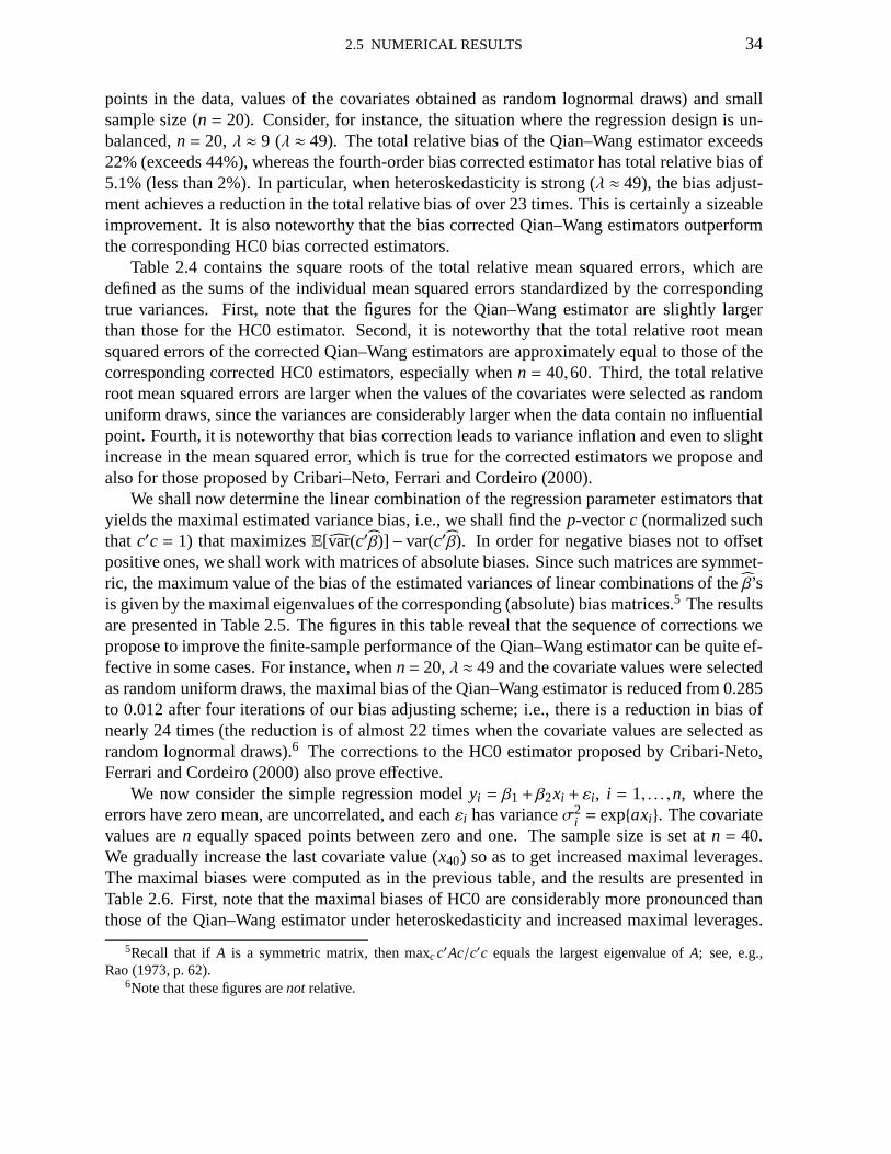
2.5 NUMERICAL RESULTS 34
points in the data, values of the covariates obtained as random lognormal draws) and smallsample size (n = 20). Consider, for instance, the situation where the regression design is un-balanced,n= 20, λ ≈ 9 (λ ≈ 49). The total relative bias of the Qian–Wang estimator exceeds22% (exceeds 44%), whereas the fourth-order bias correctedestimator has total relative bias of5.1% (less than 2%). In particular, when heteroskedasticity is strong (λ ≈ 49), the bias adjust-ment achieves a reduction in the total relative bias of over 23 times. This is certainly a sizeableimprovement. It is also noteworthy that the bias corrected Qian–Wang estimators outperformthe corresponding HC0 bias corrected estimators.
Table 2.4 contains the square roots of the total relative mean squared errors, which aredefined as the sums of the individual mean squared errors standardized by the correspondingtrue variances. First, note that the figures for the Qian–Wang estimator are slightly largerthan those for the HC0 estimator. Second, it is noteworthy that the total relative root meansquared errors of the corrected Qian–Wang estimators are approximately equal to those of thecorresponding corrected HC0 estimators, especially whenn = 40,60. Third, the total relativeroot mean squared errors are larger when the values of the covariates were selected as randomuniform draws, since the variances are considerably largerwhen the data contain no influentialpoint. Fourth, it is noteworthy that bias correction leads to variance inflation and even to slightincrease in the mean squared error, which is true for the corrected estimators we propose andalso for those proposed by Cribari–Neto, Ferrari and Cordeiro (2000).
We shall now determine the linear combination of the regression parameter estimators thatyields the maximal estimated variance bias, i.e., we shall find thep-vectorc (normalized suchthat c′c = 1) that maximizesE[var(c′β)] − var(c′β). In order for negative biases not to offsetpositive ones, we shall work with matrices of absolute biases. Since such matrices are symmet-ric, the maximum value of the bias of the estimated variancesof linear combinations of theβ’sis given by the maximal eigenvalues of the corresponding (absolute) bias matrices.5 The resultsare presented in Table 2.5. The figures in this table reveal that the sequence of corrections wepropose to improve the finite-sample performance of the Qian–Wang estimator can be quite ef-fective in some cases. For instance, whenn= 20,λ ≈ 49 and the covariate values were selectedas random uniform draws, the maximal bias of the Qian–Wang estimator is reduced from 0.285to 0.012 after four iterations of our bias adjusting scheme;i.e., there is a reduction in bias ofnearly 24 times (the reduction is of almost 22 times when the covariate values are selected asrandom lognormal draws).6 The corrections to the HC0 estimator proposed by Cribari-Neto,Ferrari and Cordeiro (2000) also prove effective.
We now consider the simple regression modelyi = β1+ β2xi + εi , i = 1, . . . ,n, where theerrors have zero mean, are uncorrelated, and eachεi has varianceσ2
i = expaxi. The covariatevalues aren equally spaced points between zero and one. The sample size is set atn = 40.We gradually increase the last covariate value (x40) so as to get increased maximal leverages.The maximal biases were computed as in the previous table, and the results are presented inTable 2.6. First, note that the maximal biases of HC0 are considerably more pronounced thanthose of the Qian–Wang estimator under heteroskedasticityand increased maximal leverages.
5Recall that if A is a symmetric matrix, then maxc c′Ac/c′c equals the largest eigenvalue ofA; see, e.g.,Rao (1973, p. 62).
6Note that these figures arenot relative.
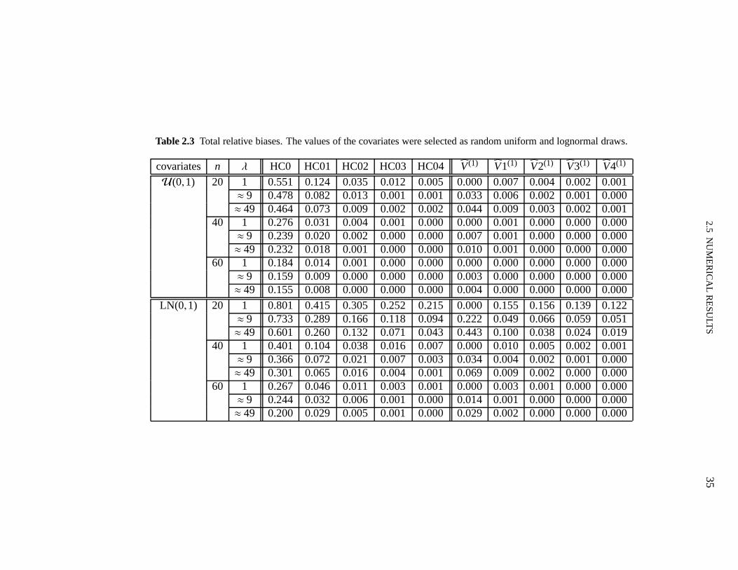
2.5
NU
ME
RIC
AL
RE
SU
LTS
35
Table 2.3 Total relative biases. The values of the covariates were selected as random uniform and lognormal draws.
covariates n λ HC0 HC01 HC02 HC03 HC04 V(1) V1(1) V2(1) V3(1) V4(1)
U(0,1) 20 1 0.551 0.124 0.035 0.012 0.005 0.000 0.007 0.004 0.002 0.001≈ 9 0.478 0.082 0.013 0.001 0.001 0.033 0.006 0.002 0.001 0.000≈ 49 0.464 0.073 0.009 0.002 0.002 0.044 0.009 0.003 0.002 0.001
40 1 0.276 0.031 0.004 0.001 0.000 0.000 0.001 0.000 0.000 0.000≈ 9 0.239 0.020 0.002 0.000 0.000 0.007 0.001 0.000 0.000 0.000≈ 49 0.232 0.018 0.001 0.000 0.000 0.010 0.001 0.000 0.000 0.000
60 1 0.184 0.014 0.001 0.000 0.000 0.000 0.000 0.000 0.000 0.000≈ 9 0.159 0.009 0.000 0.000 0.000 0.003 0.000 0.000 0.000 0.000≈ 49 0.155 0.008 0.000 0.000 0.000 0.004 0.000 0.000 0.000 0.000
LN(0,1) 20 1 0.801 0.415 0.305 0.252 0.215 0.000 0.155 0.156 0.139 0.122≈ 9 0.733 0.289 0.166 0.118 0.094 0.222 0.049 0.066 0.059 0.051≈ 49 0.601 0.260 0.132 0.071 0.043 0.443 0.100 0.038 0.024 0.019
40 1 0.401 0.104 0.038 0.016 0.007 0.000 0.010 0.005 0.002 0.001≈ 9 0.366 0.072 0.021 0.007 0.003 0.034 0.004 0.002 0.001 0.000≈ 49 0.301 0.065 0.016 0.004 0.001 0.069 0.009 0.002 0.000 0.000
60 1 0.267 0.046 0.011 0.003 0.001 0.000 0.003 0.001 0.000 0.000≈ 9 0.244 0.032 0.006 0.001 0.000 0.014 0.001 0.000 0.000 0.000≈ 49 0.200 0.029 0.005 0.001 0.000 0.029 0.002 0.000 0.000 0.000

2.5
NU
ME
RIC
AL
RE
SU
LTS
36
Table 2.4 Square roots of the total relative mean squared errors. The values of the covariates were selected as random uniform and lognormaldraws.
covariates n λ HC0 HC01 HC02 HC03 HC04 V(1) V1(1) V2(1) V3(1) V4(1)
U(0,1) 20 1 0.540 0.612 0.649 0.664 0.670 0.647 0.662 0.669 0.672 0.674≈ 9 1.173 1.348 1.413 1.433 1.438 1.408 1.429 1.437 1.440 1.440≈ 49 2.621 3.065 3.212 3.253 3.264 3.200 3.244 3.260 3.265 3.266
40 1 0.277 0.299 0.305 0.306 0.306 0.303 0.306 0.306 0.306 0.306≈ 9 0.612 0.663 0.672 0.673 0.673 0.670 0.673 0.673 0.673 0.673≈ 49 1.406 1.537 1.558 1.561 1.561 1.554 1.560 1.561 1.561 1.561
60 1 0.186 0.197 0.198 0.199 0.199 0.198 0.199 0.199 0.199 0.199≈ 9 0.413 0.437 0.440 0.440 0.440 0.439 0.440 0.440 0.440 0.440≈ 49 0.957 1.019 1.025 1.026 1.026 1.023 1.025 1.026 1.026 1.026
LN(0,1) 20 1 0.269 0.297 0.321 0.341 0.360 0.361 0.377 0.394 0.409 0.422≈ 9 0.496 0.585 0.642 0.676 0.701 0.690 0.712 0.734 0.752 0.767≈ 49 1.177 1.435 1.573 1.643 1.682 1.638 1.676 1.711 1.736 1.753
40 1 0.142 0.157 0.164 0.167 0.168 0.165 0.167 0.168 0.169 0.169≈ 9 0.263 0.293 0.302 0.305 0.306 0.302 0.305 0.306 0.306 0.306≈ 49 0.641 0.723 0.744 0.749 0.750 0.743 0.749 0.750 0.751 0.751
60 1 0.096 0.104 0.106 0.107 0.107 0.106 0.107 0.107 0.107 0.107≈ 9 0.178 0.193 0.196 0.196 0.196 0.195 0.196 0.196 0.196 0.196≈ 49 0.438 0.477 0.484 0.485 0.485 0.483 0.485 0.485 0.485 0.485

2.5
NU
ME
RIC
AL
RE
SU
LTS
37
Table 2.5 Maximal biases. The values of the covariates were selected as random uniform and lognormal draws.
covariates n λ HC0 HC01 HC02 HC03 HC04 V(1) V1(1) V2(1) V3(1) V4(1)
U(0,1) 20 1 0.208 0.052 0.016 0.006 0.003 0.000 0.004 0.002 0.001 0.001≈ 9 0.775 0.142 0.025 0.007 0.004 0.057 0.014 0.006 0.003 0.002≈ 49 2.848 0.443 0.100 0.048 0.034 0.285 0.093 0.045 0.024 0.012
40 1 0.052 0.006 0.001 0.000 0.000 0.000 0.000 0.000 0.000 0.000≈ 9 0.194 0.018 0.002 0.000 0.000 0.006 0.001 0.000 0.000 0.000≈ 49 0.712 0.055 0.006 0.001 0.001 0.032 0.005 0.001 0.000 0.000
60 1 0.023 0.002 0.000 0.000 0.000 0.000 0.000 0.000 0.000 0.000≈ 9 0.086 0.005 0.000 0.000 0.000 0.002 0.000 0.000 0.000 0.000≈ 49 0.316 0.016 0.001 0.000 0.000 0.009 0.001 0.000 0.000 0.000
LN(0,1) 20 1 0.074 0.034 0.025 0.020 0.018 0.000 0.013 0.013 0.011 0.010≈ 9 0.196 0.067 0.030 0.018 0.014 0.028 0.009 0.009 0.008 0.007≈ 49 0.892 0.323 0.128 0.053 0.022 0.131 0.047 0.021 0.010 0.006
40 1 0.018 0.004 0.001 0.001 0.000 0.000 0.000 0.000 0.000 0.000≈ 9 0.049 0.008 0.002 0.001 0.000 0.002 0.000 0.000 0.000 0.000≈ 49 0.223 0.040 0.008 0.002 0.000 0.012 0.003 0.001 0.000 0.000
60 1 0.008 0.001 0.000 0.000 0.000 0.000 0.000 0.000 0.000 0.000≈ 9 0.022 0.002 0.000 0.000 0.000 0.001 0.000 0.000 0.000 0.000≈ 49 0.099 0.012 0.002 0.000 0.000 0.003 0.000 0.000 0.000 0.000
2.5 NUMERICAL RESULTS 38
For instance, under the strongest level of heteroskedasticity (λ ≈ 49) andhmax = 0.289, themaximal biases of these two estimators are 1.587 and 0.356, respectively. Second, note thatcorrections proposed in this chapter can be quite effective under unequal error variances. As anillustration, consider again the setting under strongest heteroskedasticity and maximal leverageof almost twice the threshold value 3p/n= 0.150. The bias of the Qian–Wang estimator shrinksfrom 0.356 to 0.024 after four iterations of our bias correcting scheme, which amounts to a biasreduction of nearly 15 times.
Our focus lies in obtaining accurate (nearly unbiased) point estimates of variances and co-variances of OLSEs. We note, however, that such estimates are oftentimes used for performinginferences on the regression parameters. We have run a smallMonte Carlo experiment in orderto evaluate the finite sample performance of quasi-t tests based on the HC0 and Qian–Wang es-timators and also on their corrected versions up to four iterations of the bias correcting schemes.The regression model isyi = β1+β2xi2+β3xi3+εi , i = 1, . . . ,n. The errors are independent andnormally distributed with zero mean and varianceσ2
i = exp(axi1). The interest lies in the testof H0 : β3 = 0 versusH1 : β3 , 0. The covariate values were obtained as random draws fromthe t3 distribution, there are leverage points,n = 20, λ ≈ 49 and the number of Monte Carloreplications was 10,000. Here,hmax= 5.66p/n, so there is an observation with very high lever-age. The null rejection rates at the 5% nominal level of the HC0 test and of the tests basedon standard errors obtained from the corrected HC0 estimators (one, two, there and four itera-tions of the bias correcting scheme) were, respectively, 17.46%, 16.20%, 18.31%, 18.71% and15.97%; the corresponding figures for the Qian–Wang test andthe four tests based on the cor-rected Qian–Wang estimators were 11.66%, 7.07%, 6.44%, 5.87% and 5.71%. The tests basedon the corrected Qian–Wang estimators were also less size-distorted than the Qian–Wang testwhenλ = 1 (15.28% for the Qian–Wang test and 8.35%, 7.59%, 7.04% and 6.58% for the testsbased on the corrected standard errors) andλ ≈ 9 (Qian–Wang: 12.50%; corrected: 6.86%,6.25%, 5.93% and 5.60%). We thus notice that the finite samplecorrections we propose mayyield more accurate hypothesis testing inference in addition to more accurate point estimates.Even though we do not present all Monte Carlo results, we notethat the tests based on theQian–Wang estimator and its corrected versions displayed similar behavior for larger samplesizes (40 observations or more).
We have also performed simulations in which the wild bootstrap was used to obtain a criticalvalue for the HC3-based quasi-t test statistic. As suggested by Flachaire (2005), resampling inthe wild bootstrap scheme was performing using the Rademacher population. The number ofMonte Carlo replications was 5,000 and there were 500 bootstrap replicates for each MonteCarlo sample. The null rejection rates at the 5% nominal level for n = 20, covariate valuesobtained ast3 random draws andλ = 1, λ ≈ 9 andλ ≈ 49 were 17.62%, 14.76% and 11.34%,respectively. We noticed that the wild bootstrap worked well in the balanced case (no leveragepoint in the data) for all sample sizes. In the unbalanced case (leveraged data), it only yieldedsatisfactory results forn≥ 60.7
7The wild bootstrap performed considerably better under less extreme leverage, e.g., whenhmax< 4p/n.

2.5
NU
ME
RIC
AL
RE
SU
LTS
39
Table 2.6 Maximal biases,n = 40, single regression model with covariate values chosen asa sequence of equally spaced points in the standardunit interval; the last point is gradually increased in order for the maximal leverage to increase; here, 3p/n= 0.150.
λ hmax HC0 HC01 HC02 HC03 HC04 V(1) V1(1) V2(1) V3(1) V4(1)
1 0.096 0.025 0.002 0.000 0.000 0.000 0.000 0.000 0.000 0.000 0.0000.154 0.026 0.003 0.000 0.000 0.000 0.000 0.000 0.000 0.000 0.0000.220 0.028 0.005 0.002 0.001 0.000 0.000 0.001 0.000 0.000 0.0000.289 0.033 0.010 0.004 0.002 0.001 0.000 0.002 0.001 0.000 0.0000.357 0.039 0.016 0.009 0.005 0.003 0.000 0.004 0.003 0.002 0.0010.422 0.044 0.023 0.015 0.010 0.007 0.000 0.007 0.005 0.004 0.0020.482 0.049 0.030 0.022 0.016 0.012 0.000 0.011 0.009 0.006 0.005
≈ 9 0.096 0.109 0.011 0.001 0.000 0.000 0.001 0.000 0.000 0.000 0.0000.154 0.126 0.023 0.005 0.001 0.000 0.007 0.002 0.001 0.000 0.0000.220 0.197 0.063 0.024 0.009 0.004 0.024 0.012 0.005 0.002 0.0010.289 0.296 0.133 0.065 0.033 0.016 0.055 0.033 0.017 0.008 0.0040.357 0.405 0.226 0.133 0.079 0.047 0.098 0.068 0.041 0.024 0.0140.422 0.495 0.320 0.214 0.143 0.096 0.144 0.113 0.077 0.052 0.0350.482 0.571 0.410 0.301 0.221 0.163 0.192 0.165 0.123 0.090 0.066
≈ 49 0.096 0.482 0.052 0.006 0.001 0.000 0.012 0.002 0.000 0.000 0.0000.154 0.588 0.126 0.033 0.009 0.003 0.049 0.015 0.004 0.001 0.0000.220 1.006 0.358 0.139 0.055 0.022 0.160 0.069 0.028 0.011 0.0040.289 1.587 0.757 0.376 0.187 0.094 0.356 0.191 0.097 0.048 0.0240.357 2.170 1.255 0.741 0.439 0.260 0.611 0.386 0.230 0.136 0.0810.422 2.700 1.787 1.197 0.803 0.539 0.901 0.640 0.432 0.290 0.1940.482 3.117 2.274 1.671 1.230 0.905 1.189 0.922 0.681 0.501 0.369
2.6 EMPIRICAL ILLUSTRATIONS 40
2.6 Empirical illustrations
In what follows we shall present two empirical applicationsthat use real data. In the first appli-cation, the dependent variable (y) is per capita spending on public schools and the independentvariables,x andx2, are per capita income by state in 1979 in the United States and its square;income is scaled by 10−4. Wisconsin was not considered since it had missing data, andWash-ington D.C. was included. The data are presented in Greene (1997, Table 12.1, p. 541) andtheir original source is the U.S. Department of Commerce. The regression model is
yi = β1+β2xi +β3x2i +εi , i = 1, . . . ,50.
The ordinary least squares estimates for the linear parameters areβ1 = 832.91, β2 = −1834.20andβ3 = 1587.04. The Breusch–Pagan–Godfrey test of homoskedasticity rejects this hypoth-esis at the 1% nominal level, thus indicating that there is heteroskedasticity in the data. Itshould be noted that the data contain three leverage points,namely: Alaska, Mississipi andWashington, D.C. (their leverage measures are 0.651, 0.200and 0.208, respectively; note that3p/n= 0.180).
In Table 2.7 we present the standard errors for the regression parameter estimates. We con-sider four designs: (i) case 1: all 50 observations were used; (ii) case 2: Alaska (the strongestleverage point) was removed from the data (n= 49); (iii) case 3: Alaska and Washington D.C.were removed from the data (n = 48); (iv) case 4: Alaska, Washington D.C. and Mississipiwere removed from data (n= 47). Table 2.8 contains information on the detection of leveragepoints in these four situations.
The figures in Table 2.7 reveal that when all 50 observations are used (case 1, three leveragepoints in the data), the HC0 standard errors are considerably smaller than the Qian–Wang stan-dard errors; the same pattern holds for their correspondingbias adjusted versions. For instance,the standard errors ofβ3 are 829.99 (HC0) and 1348.36 (Qian–Wang). The same discrepancyholds for case 2, i.e., when Alaska is removed from the data. The HC0 and Qian–Wang stan-dard errors, however, are somewhat similar in cases 3 (Alaska and Washington D.C. are not inthe data) and 4 (Alaska, Mississipi and Washington D.C. are not in the data). In these cases,the ratios betweenhmax and 3p/n are smaller than 2. It is also noteworthy that in case 4 thefourth-order corrected HC0 and Qian–Wang standard errors are nearly equal.
It is particularly interesting to note that a scatterplot shows a satisfactorily linear scatterexcept for a single high leverage point: Alaska. The HC0 standard error ofβ3 equals 829.99when the sample contains all 50 observations (β3= 1587.04); this standard error is highly biasedin favor of the quadratic model specification. The Qian–Wangstandard error equals 1348.36,thus indicating greater uncertainty relative to the possible nonlinear effect of xt onE(yt). Ourfourth-order corrected estimate is even greater: 1385.77.
The data for the second application were obtained from Cagan(1974, Table 1, p. 4). Thedependent variable (y) is the percent rate of change in stock prices (% per year) andthe in-dependent variable (x) is the percent rate of change in consumer prices (% per year). Thereare observations for 20 countries (n = 20) in the period that goes from the post-World War IIthrough 1969. The regression model is
yi = β1+β2xi +εi , i = 1, . . . ,n.
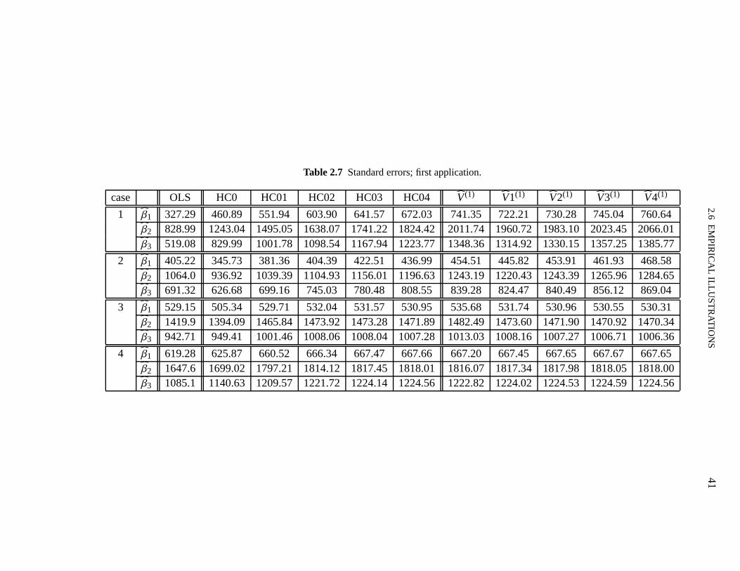
2.6
EM
PIR
ICA
LIL
LU
ST
RA
TIO
NS
41
Table 2.7 Standard errors; first application.
case OLS HC0 HC01 HC02 HC03 HC04 V(1) V1(1) V2(1) V3(1) V4(1)
1 β1 327.29 460.89 551.94 603.90 641.57 672.03 741.35 722.21 730.28 745.04 760.64β2 828.99 1243.04 1495.05 1638.07 1741.22 1824.42 2011.74 1960.72 1983.10 2023.45 2066.01β3 519.08 829.99 1001.78 1098.54 1167.94 1223.77 1348.36 1314.92 1330.15 1357.25 1385.77
2 β1 405.22 345.73 381.36 404.39 422.51 436.99 454.51 445.82 453.91 461.93 468.58β2 1064.0 936.92 1039.39 1104.93 1156.01 1196.63 1243.19 1220.43 1243.39 1265.96 1284.65β3 691.32 626.68 699.16 745.03 780.48 808.55 839.28 824.47 840.49 856.12 869.04
3 β1 529.15 505.34 529.71 532.04 531.57 530.95 535.68 531.74 530.96 530.55 530.31β2 1419.9 1394.09 1465.84 1473.92 1473.28 1471.89 1482.49 1473.60 1471.90 1470.92 1470.34β3 942.71 949.41 1001.46 1008.06 1008.04 1007.28 1013.03 1008.16 1007.27 1006.71 1006.36
4 β1 619.28 625.87 660.52 666.34 667.47 667.66 667.20 667.45 667.65 667.67 667.65β2 1647.6 1699.02 1797.21 1814.12 1817.45 1818.01 1816.07 1817.34 1817.98 1818.05 1818.00β3 1085.1 1140.63 1209.57 1221.72 1224.14 1224.56 1222.82 1224.02 1224.53 1224.59 1224.56
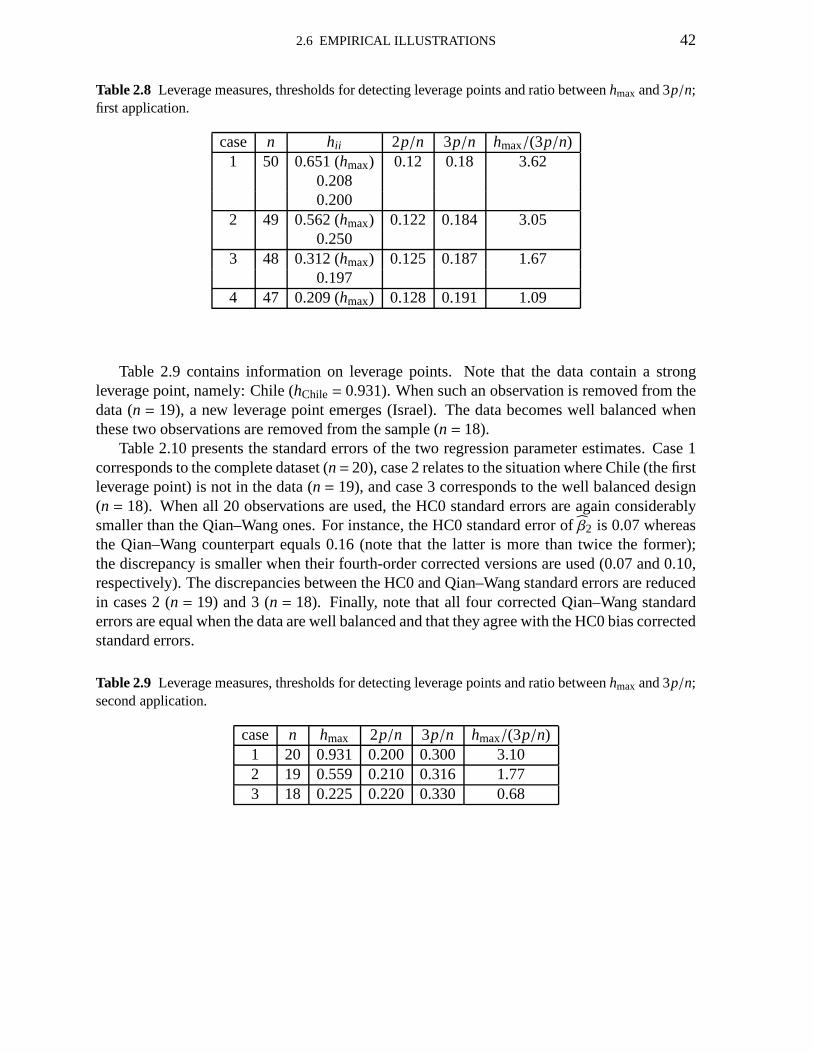
2.6 EMPIRICAL ILLUSTRATIONS 42
Table 2.8 Leverage measures, thresholds for detecting leverage points and ratio betweenhmax and 3p/n;first application.
case n hii 2p/n 3p/n hmax/(3p/n)1 50 0.651 (hmax) 0.12 0.18 3.62
0.2080.200
2 49 0.562 (hmax) 0.122 0.184 3.050.250
3 48 0.312 (hmax) 0.125 0.187 1.670.197
4 47 0.209 (hmax) 0.128 0.191 1.09
Table 2.9 contains information on leverage points. Note that the data contain a strongleverage point, namely: Chile (hChile= 0.931). When such an observation is removed from thedata (n = 19), a new leverage point emerges (Israel). The data becomeswell balanced whenthese two observations are removed from the sample (n= 18).
Table 2.10 presents the standard errors of the two regression parameter estimates. Case 1corresponds to the complete dataset (n= 20), case 2 relates to the situation where Chile (the firstleverage point) is not in the data (n= 19), and case 3 corresponds to the well balanced design(n = 18). When all 20 observations are used, the HC0 standard errors are again considerablysmaller than the Qian–Wang ones. For instance, the HC0 standard error ofβ2 is 0.07 whereasthe Qian–Wang counterpart equals 0.16 (note that the latteris more than twice the former);the discrepancy is smaller when their fourth-order corrected versions are used (0.07 and 0.10,respectively). The discrepancies between the HC0 and Qian–Wang standard errors are reducedin cases 2 (n = 19) and 3 (n = 18). Finally, note that all four corrected Qian–Wang standarderrors are equal when the data are well balanced and that theyagree with the HC0 bias correctedstandard errors.
Table 2.9 Leverage measures, thresholds for detecting leverage points and ratio betweenhmax and 3p/n;second application.
case n hmax 2p/n 3p/n hmax/(3p/n)1 20 0.931 0.200 0.300 3.102 19 0.559 0.210 0.316 1.773 18 0.225 0.220 0.330 0.68
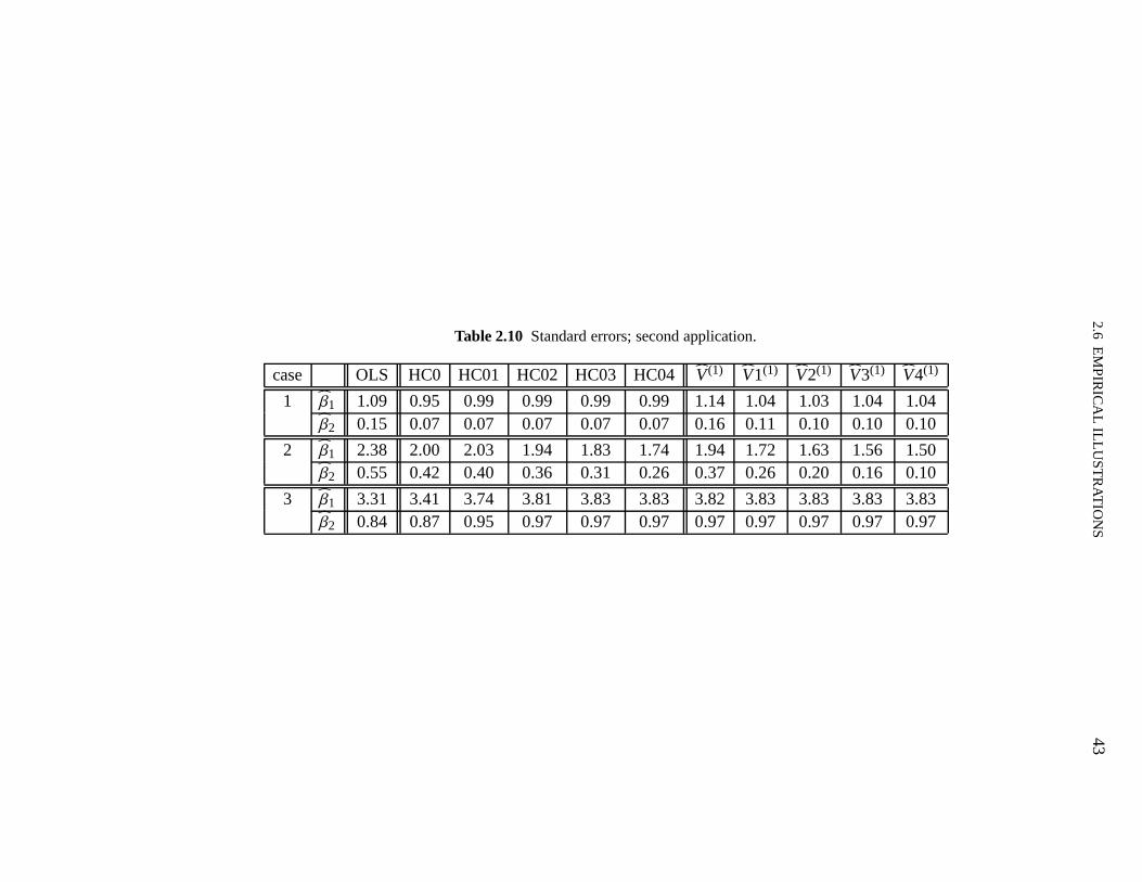
2.6
EM
PIR
ICA
LIL
LU
ST
RA
TIO
NS
43
Table 2.10 Standard errors; second application.
case OLS HC0 HC01 HC02 HC03 HC04 V(1) V1(1) V2(1) V3(1) V4(1)
1 β1 1.09 0.95 0.99 0.99 0.99 0.99 1.14 1.04 1.03 1.04 1.04β2 0.15 0.07 0.07 0.07 0.07 0.07 0.16 0.11 0.10 0.10 0.10
2 β1 2.38 2.00 2.03 1.94 1.83 1.74 1.94 1.72 1.63 1.56 1.50β2 0.55 0.42 0.40 0.36 0.31 0.26 0.37 0.26 0.20 0.16 0.10
3 β1 3.31 3.41 3.74 3.81 3.83 3.83 3.82 3.83 3.83 3.83 3.83β2 0.84 0.87 0.95 0.97 0.97 0.97 0.97 0.97 0.97 0.97 0.97
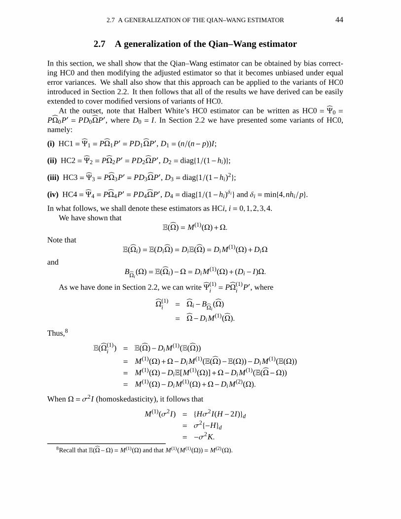
2.7 A GENERALIZATION OF THE QIAN–WANG ESTIMATOR 44
2.7 A generalization of the Qian–Wang estimator
In this section, we shall show that the Qian–Wang estimator can be obtained by bias correct-ing HC0 and then modifying the adjusted estimator so that it becomes unbiased under equalerror variances. We shall also show that this approach can beapplied to the variants of HC0introduced in Section 2.2. It then follows that all of the results we have derived can be easilyextended to cover modified versions of variants of HC0.
At the outset, note that Halbert White’s HC0 estimator can bewritten as HC0= Ψ0 =
PΩ0P′ = PD0ΩP′, whereD0 = I . In Section 2.2 we have presented some variants of HC0,namely:
(i) HC1= Ψ1 = PΩ1P′ = PD1ΩP′, D1 = (n/(n− p))I ;
(ii) HC2= Ψ2 = PΩ2P′ = PD2ΩP′, D2 = diag1/(1−hi);
(iii) HC3= Ψ3 = PΩ3P′ = PD3ΩP′, D3 = diag1/(1−hi)2;
(iv) HC4= Ψ4 = PΩ4P′ = PD4ΩP′, D4 = diag1/(1−hi)δi andδi =min4,nhi/p.In what follows, we shall denote these estimators as HCi, i = 0,1,2,3,4.
We have shown thatE(Ω) = M(1)(Ω)+Ω.
Note thatE(Ωi) = E(DiΩ) = DiE(Ω) = Di M
(1)(Ω)+DiΩ
andBΩi
(Ω) = E(Ωi)−Ω = Di M(1)(Ω)+ (Di − I )Ω.
As we have done in Section 2.2, we can writeΨ(1)i = PΩ(1)
i P′, where
Ω(1)i = Ωi −B
Ωi(Ω)
= Ω−Di M(1)(Ω).
Thus,8
E(Ω(1)i ) = E(Ω)−Di M
(1)(E(Ω))
= M(1)(Ω)+Ω−Di M(1)(E(Ω)−E(Ω))−Di M
(1)(E(Ω))
= M(1)(Ω)−DiE[M(1)(Ω)] +Ω−Di M(1)(E(Ω−Ω))
= M(1)(Ω)−Di M(1)(Ω)+Ω−Di M
(2)(Ω).
WhenΩ = σ2I (homoskedasticity), it follows that
M(1)(σ2I ) = Hσ2I (H −2I )d= σ2−Hd= −σ2K.
8Recall thatE(Ω−Ω) = M(1)(Ω) and thatM(1)(M(1)(Ω)) = M(2)(Ω).
2.7 A GENERALIZATION OF THE QIAN–WANG ESTIMATOR 45
Additionally,
M(2)(σ2I ) = M(1)(M(1)(σ2I ))
= H(−σ2K)(H −2I )d= σ2−HKH +2KKd.
(Note that we have used the fact thatH is idempotent, thatK = (H)d and that (HK)d = (KK)d.)Therefore, under homoskedasticity,
E(Ω(1)i ) = −σ2K +Diσ
2K +σ2I −σ2Di−HKH +2KKd= σ2[(I −K)+Di K +HKH −2KKd]
= σ2Ai ,
whereAi = (I −K)+DiK +HKH −2KKd. We shall now obtain the expected value ofΨ(1)i
whenΩ = σ2I (homoskedastic errors):
E(Ψ(1)i ) = E(PΩ(1)
i P′)
= σ2PAiP′.
Hence, the estimatorΨ
(1)iA = PΩ(1)
iA P′ = PΩ(1)i A−1
i P′
is unbiased:
E(Ψ(1)iA ) = E(PΩ(1)
i A−1i P′)
= Pσ2AiA−1i P′
= Pσ2IP′
= PΩP′
= Ψ.
It is noteworthy that the Qian–Wang estimator given in Section 2.3 is a particular case ofΨ
(1)iA wheni = 0, i.e., whenD0 = I . Indeed, note that
Ψ(1)0A = PΩ(1)
0 A−10 P′ = PD(1)P′ = V(1),
whereΩ(1)0 = Ω−M(1)(Ω) andA0 = I +HKH −2KKd.9
We shall now derive the bias ofΨ(1)iA under heteroskedasticity. Note that
BΩ
(1)iA
(Ω) = E(Ω(1)iA )−Ω
= [M(1)(Ω)−Di M(1)(Ω)+Ω−Di M
(2)(Ω)]A−1i −Ω
= Ω(A−1i − I )+ (I −Di)M
(1)(Ω)A−1i −Di M
(2)(Ω)A−1i .
9In Section 2.2,Ω(1)0 was denoted asΩ(1).
2.7 A GENERALIZATION OF THE QIAN–WANG ESTIMATOR 46
Hence,
BΨ
(1)iA
(Ω) = E(Ψ(1)iA )−Ψ
= P[BΩ
(1)iA
(Ω)]P′.
This is a closed-form expression for the bias of the class of estimators we have considered inthis section. In particular, it can be used to further bias correct the estimators. Indeed, it isimportant to note that all of the results in Sections 2.3 and 2.4 can be easily extended to themore general class of estimators considered here.
We shall obtain a sequence of bias adjusted estimators starting from the modified estimator
Ψ(1)iA = PΩ(1)
iA P′ = PΩ(1)i A−1
i P′,
for i = 1, . . . ,4. (The casei = 0 was already addressed when we bias corrected the Qian–Wangestimator. Note that the results presented below agree withthe ones obtained forV(1) when welet D0 = I .) Let Gi = A−1
i .The one iteration bias adjusted estimator is
Ω(2)iA = Ω
(1)iA −B
Ω(1)iA
(Ω)
= (Ω−Di M(1)(Ω))Gi −B
Ω(1)iA
(Ω)
= ΩGi −Di M(1)(Ω)Gi − (I −Di)M
(1)(Ω)Gi +Di M(2)(Ω)Gi − Ω(Gi − I )
= Ω−M(1)(Ω)Gi +Di M(2)(Ω)Gi .
Its bias can be expressed as
BΩ
(2)iA
(Ω) = E(Ω(2)iA )−Ω
= E(Ω−M(1)(Ω)Gi +Di M(2)(Ω)Gi)−Ω
= E(Ω−Ω)−E(M(1)(Ω)−M(1)(Ω))Gi −M(1)(Ω)Gi +
+ DiE(M(2)(Ω)−M(2)(Ω))Gi +Di M(2)(Ω)Gi
= −M(1)(Ω)(Gi − I )− (I −Di)M(2)(Ω)Gi +Di M
(3)(Ω)Gi .
After k iterations of the bias correcting scheme we obtain
Ω(k)iA = 1(k>1)×M(0)(Ω)+1(k>2)×
k−2∑
j=1
(−1) j M( j)(Ω)
+ (−1)k−1M(k−1)(Ω)Gi + (−1)kDi M(k)(Ω)Gi ,
k= 1,2, . . .. The bias of this estimator is given by
BΩ
(k)iA
(Ω) = (−1)k−1M(k−1)(Ω)(Gi − I )
+ (−1)k−1(I −Di)M(k)(Ω)Gi + (−1)kDi M
(k+1)(Ω)Gi ,
2.7 A GENERALIZATION OF THE QIAN–WANG ESTIMATOR 47
k= 1,2, . . ..We can now define a sequenceΨ(k)
iA ,k= 1,2, . . . of bias adjusted estimators forΨ, where
Ψ(k)iA = PΩ(k)
iA P′
is thekth order bias corrected estimator ofΨ and its bias is
BΨ
(k)iA
(Ω) = P[BΩ
(k)iA
(Ω)]P′.
Next, we shall investigate the order of the bias ofΩ(k)iA given above fork = 1,2, . . .. Recall
thatGi =A−1i with Ai = (I −K)+Di K +HKH −2KKd. Recall also thatΩ=O(n0), P=O(n−1),
H = O(n−1). Let us obtain the order ofGi , i = 1, . . . ,4. Note thatI −K = O(n0). Additionally,for i = 1, . . . ,4, it is easy to show thatDi =O(n0) andI −Di =O(n−1). Also, K+HKH −2KK =O(n−1). Thus,G−1
i = O(n0) and, as a consequence,Gi = O(n0). Let us now move to the orderof Gi − I . Let d j , b j andg j denote thejth diagonal elements ofDi , K +HKH −2KKd andGi ,respectively. Hence,
g j −1=1
(1−h j)+d jb j−1=
h j −d jb j
1−h j +d jb j.
Note thath j −d jb j =O(n−1) and that the order of the denominator isO(n0) since it is a diagonalelement ofAi . Therefore,Gi − I = O(n−1). Now recall thatM(k−1)(Ω) = O(n−(k−1)), M(k)(Ω) =O(n−k) and M(k+1)(Ω) = O(n−(k+1)). We then obtain thatB
Ω(k)iA
(Ω) is of orderO(n−k) which
implies thatBΨ
(k)iA
(Ω) =O(n−(k+1)), i = 1, . . . ,4.
By lettingk= 1, we see that the order of the biases of the estimators we proposed in this sec-tion is larger than that ofΨ(1)
0A (the Qian-Wang estimator), which we have shown to beO(n−3). Italso follows that in order to obtain the same precision with the bias corrected estimators givenhere relative to those given in Section 2.3 one needs to go onestep further in the sequence ofbias adjustment iterations. In that sense, even though the Qian–Wang estimator is a particularcase of the class of covariance matrix estimators we proposehere, the results relative to biasadjustment given in this section do not generalize those obtained for the Qian–Wang estima-tor. This is so because the orders of the corrected estimators for i = 1, . . . ,4 differ from thecorresponding orders wheni = 0.
We shall now use the estimators
Ψ(1)iA = PΩ(1)
iA P′ = PΩ(1)i A−1
i P′, i = 0, . . . ,4,
to estimate the variance of linear combinations of the components inβ. Let c be ap-vector ofscalars. The estimator ofΦ = var(c′β) is
Φ(1)iA = c′Ψ(1)
iA c
= c′PΩ(1)i GiP
′c
= c′P[Ω−Di M(1)(Ω)]GiP
′c
= c′PΩGiP′c−c′PDi M
(1)(Ω)GiP′c
= c′PG1/2i ΩG1/2
i P′c−c′PD1/2i G1/2
i M(1)(Ω)G1/2i D1/2
i P′c.

2.7 A GENERALIZATION OF THE QIAN–WANG ESTIMATOR 48
Now let wi =G1/2i P′c, vi =G1/2
i D1/2i P′c, Wi = (wiw′i )d andVi = (viv′i )d. We then have
Φ(1)iA = w′i Ωwi −v′i M
(1)(Ω)vi
= ε′Wi ε− ε′[M(1)(Vi)]ε
= ε′(Wi −M(1)(Vi))ε
= ε′Q(1)iA ε,
whereQ(1)iA =Wi −M(1)(Vi).
It is possible to writeΦ(1)iA as a quadratic form in a random vectora which has zero mean
and unit covariance:Φ
(1)iA = a′C(1)
iA a,
whereC(1)iA = Ω
1/2(I −H)Q(1)iA (I −H)Ω1/2. For simplicity of notation, letC(1)
iA =CiA. Followingthe arguments outlined in Section 2.4, we can show that
var(Φ(1)iA ) = var(a′CiAa) = 2tr(C2
iA)
when the errors are independent and normally distributed.In what follows, we shall report the results of a small numerical evaluation using the same
two-covariate regression model used in Section 2.5. In particular, we report the total relativebiases of the bias corrected versions of the modified HC0, HC1, HC2, HC3 and HC4 esti-mators; the modification consists of multiplying these estimators byA−1
i so that they become
unbiased under homoskedasticity. The results are displayed in Table 2.11. Note thatΨ(1)0A is the
Qian–Wang estimatorV(1) (see Table 2.3). It is noteworthy that under well balanced data, thetotal relative biases of the corrected modified HC1 through HC4 estimators are smaller thanthose of the Qian–Wang estimator. Under leveraged data, small sample size (n= 20) and het-eroskedasticity (λ ≈ 9 andλ ≈ 49), the corrected modified HC4 estimator is considerably lessbiased than the corrected modified HC0 (Qian–Wang) estimator. For instance, the total relativebiases of the later underλ ≈ 9 andλ ≈ 49 are 0.222 and 0.443, respectively, whereas the corre-sponding biases of the former are 0.025 and 0.025; under strong heteroskedatisticity, the biasof the corrected modified HC4 estimator is nearly 18 times smaller than that of the Qian–Wangestimator.
Finally, we shall revisit the empirical application that uses data on per capita spending onpublic schools (Section 2.6). The standard errors obtainedusing two of the estimators proposedin this section (corrected using up to three iterations) aregiven in Table 2.12; these resultsare to be compared to those in Table 2.7. In particular, we present standard errors obtainedfrom the HC3 (Davidson and MacKinnon, 1993) and HC4 (Cribari–Neto, 2004) estimators andalso heteroskedasticity-robust standard errors from our modified versions of these estimatorsand their first three corrected variants. We note that the standard errors given here are largerthan those obtained using White’s estimator and its corrected versions, and also larger thantheir Qian–Wang (uncorrected and corrected) counterpartsin the presence of leverage points(cases 1 and 2). In particular, note the standard errors ofβ3 when the data contain all 50observations (three iterations of the bias correcting scheme): 1487.68 and 1545.93 (1167.94

2.7 A GENERALIZATION OF THE QIAN–WANG ESTIMATOR 49
Table 2.11 Total relative biases for the corrected estimatorsΨ(1)iA , i = 0,1, . . . ,4, which are unbiased
under homoscedasticity. The values of the covariates were selected as random uniform and lognormaldraws.
covariates n λ Ψ(1)0A Ψ
(1)1A Ψ
(1)2A Ψ
(1)3A Ψ
(1)4A
U(0,1) 20 1 0.000 0.000 0.000 0.000 0.000≈ 9 0.033 0.027 0.022 0.009 0.012≈ 49 0.044 0.036 0.030 0.015 0.024
40 1 0.000 0.000 0.000 0.000 0.000≈ 9 0.007 0.006 0.004 0.001 0.002≈ 49 0.010 0.008 0.006 0.003 0.005
60 1 0.000 0.000 0.000 0.000 0.000≈ 9 0.003 0.002 0.002 0.000 0.001≈ 49 0.004 0.003 0.003 0.001 0.002
LN(0,1) 20 1 0.000 0.000 0.000 0.000 0.000≈ 9 0.222 0.208 0.157 0.085 0.025≈ 49 0.443 0.413 0.306 0.156 0.025
40 1 0.000 0.000 0.000 0.000 0.000≈ 9 0.034 0.029 0.017 0.002 0.037≈ 49 0.069 0.060 0.037 0.004 0.073
60 1 0.000 0.000 0.000 0.000 0.000≈ 9 0.014 0.012 0.007 0.002 0.018≈ 49 0.029 0.025 0.014 0.003 0.035
2.7
AG
EN
ER
AL
IZA
TIO
NO
FT
HE
QIA
N–
WA
NG
ES
TIM
AT
OR
50
Table 2.12 Standard errors; modified and corrected estimators:Ψ(i)3A andΨ(i)
4A, i = 1, . . . ,4; first application.
case HC3 Ψ(1)3A Ψ
(2)3A Ψ
(3)3A Ψ
(4)3A HC4 Ψ
(1)4A Ψ
(2)4A Ψ
(3)4A Ψ
(4)4A
1 β1 1095.00 836.07 811.58 810.32 816.41 3008.01 877.89 850.95 845.81 848.29β2 2975.41 2270.31 2204.41 2201.27 2217.96 8183.19 2384.47 2311.75 2297.97 2304.82β3 1995.24 1522.06 1478.41 1476.47 1487.68 5488.93 1598.76 1550.44 1541.32 1545.93
2 β1 594.80 485.52 483.52 485.60 487.75 1239.75 506.35 509.48 507.75 506.03β2 1630.15 1330.58 1325.49 1331.55 1337.73 3414.20 1389.70 1397.94 1393.26 1388.60β3 1103.03 899.90 896.69 901.00 905.35 2320.83 941.13 946.55 943.40 940.26
3 β1 577.11 531.42 530.54 530.25 530.13 613.29 524.21 528.47 529.19 529.57β2 1593.62 1473.01 1470.92 1470.21 1469.92 1688.73 1455.63 1465.90 1467.64 1468.54β3 1087.41 1007.94 1006.71 1006.29 1006.11 1150.05 997.58 1003.71 1004.73 1005.27
4 β1 707.15 668.18 667.81 667.69 667.65 725.74 668.14 667.69 667.57 667.57β2 1925.44 1819.43 1818.44 1818.10 1817.99 1980.52 1819.39 1818.12 1817.77 1817.79β3 1297.35 1225.53 1224.85 1224.63 1224.55 1337.81 1225.55 1224.65 1224.40 1224.41
2.8 CONCLUDING REMARKS 51
and 1357.25 for the two third-order corrected standard errors in Table 2.7). That is, the newstandard errors suggest that there is even more uncertaintyinvolved in the estimation ofβ3
than the standard errors reported in the previous section. (Recall thatβ3 = 1587.042.) Asnoted earlier, a scatterplot shows a satisfactorily linearscatter except for a single high leveragepoint: Alaska. The standard errors reported in Table 2.12 signal that the estimation of thequadratic income effect is highly uncertain, since it seems to be mostly driven bya single point(Alaska). It is also noteworthy that the HC4 estimator seemsto be largely positively biased (inthe opposite direction of HC0) and that iteration of the biascorrecting scheme coupled with theproposed modification yields standard errors more in line with what one would expect basedon the remaining estimates; e.g., the standard error ofβ3 is reduced from 5488.93 to 1598.76.
2.8 Concluding remarks
In this chapter we derived a sequential bias correction scheme to the heteroskedasticity-consis-tent covariance matrix estimator proposed by Qian and Wang (2001). The corrections are suchthat the order of the bias decreases as we move along the sequence. The numerical evidenceshowed that the gain in precision can be substantial when oneuses the adjusted versions ofthe estimator. It has also been shown that the corrected Qian–Wang estimators are typicallyless biased than the respective corrected HC0 (White) estimators. We have also proposed ageneral class of heteroskedasticity-consistent covariance matrix estimators which generalizesthe Qian–Wang estimator. We have shown that the sequential bias adjustment proposed for theQian–Wang estimator can be easily extended to the more general class of estimators we haveproposed.
C 3
Inference under heteroskedasticity: numericalevaluation
3.1 Introduction
The linear regression model is commonly used by practitioners to model the relationship be-tween a variable of interest and a set of explanatory or independent variables. In particular, themean of the response is a linear function of a finite number of regression parameters, each mul-tiplying a different covariate. The mean of the dependent variable (variable of interest) is thusaffected by other variables. It is commonly assumed, however, that the conditional varianceof the response is constant. If we view the response as the sumof a linear predictor (whichinvolves unknown parameters and covariates) and a zero meanunobservable error term, thatamounts to assuming that all errors share the same variance,which is known as homoskedas-ticity. In many applications, however, the errors are heteroskedastic, i.e., their variances are notconstant. The ordinary least squares estimator (OLSE) of the vector of regression parametersremains unbiased, consistent and asymptotically normal under unequal error variances. Nev-ertheless, its usual covariance matrix estimator, from which we obtain standard errors for theregression parameter estimates, is no longer valid. The standard practice is to base inferenceon standard errors obtained from a heteroskedasticity-consistent covariance matrix estimator(HCCME) which has the property of being consistent regardless of whether homoskedastic-ity holds; indeed, the estimator is asymptotically correctunder heteroskedasticity of unknownform. The most commonly used HCCME was proposed by Halbert White in an influentialand highly cited paper published nearly 30 years ago (White,1980). White’s estimator, alsoknown as HC0, can be, however, quite biased in samples of typical sizes; see, e.g., Cribari–Neto (2004), Cribari–Neto and Zarkos (1999, 2001), Long andErvin (2000) and MacKinnonand White (1985). In particular, substantial downward biascan occur for regression designscontaining points of high leverage (Chesher and Jewitt, 1987). The use of White’s varianceestimator may thus lead one to find spurious relationships between the variable of interest andother variables.
A few variants of the White (HC0) estimator were proposed in the literature. They in-clude the HC1 (Hinkley, 1977), HC2 (Horn, Horn and Duncan, 1975) and HC3 (Davidson andMacKinnon, 1993) estimators. The Monte Carlo evidence in Long and Ervin (2000) favorsHC3-based inference. According to the authors (p. 223), “for samples less than 250, HC3should be used.” They “recommend that HC3-based tests should be used routinely for testingindividual coefficients in the linear regression model.”
Four new promissing HCCMEs were recently proposed, namely:theV1 andV2 estimators
52
3.1 INTRODUCTION 53
of Qian and Wang (2001), the HC4 estimator of Cribari–Neto (2004) and the HC5 estimatorof Cribari–Neto et al. (2007). A nice feature of Qian and Wang’s V1 andV2 estimators is thatthey are unbiased under homoskedasticity. It is also possible to show that, under heteroskedas-ticity, the bias ofV1 converges to zero faster than that of HC0. Using Monte Carlo simulations,Cribari–Neto (2004) showed that hypothesis testing based on HC4 can even outperform infer-ence obtained from a computationally intensive double bootstrapping scheme. Cribari–Netoet al. (2007) argue that HC5-based inference should be preferred when the data contain strongleverage points.
Standard errors that deliver asymptotically correct inference even when the errors of themodel do not share the same variance are extremely useful in applications. Davidson andMacKinnon (2004, p. 199) note that “these heteroskedasticity-consistent standard errors, whichmay also be referred to as heteroskedasticity-robust, are often enormously useful.” JeffreyWooldridge agrees (Wooldridge, 2000, p. 249): “In the last two decades, econometricians havelearned to adjust standard errors,t, F andLM statistics so that they are valid in the presence ofheteroskedasticity of unknown form. This is very convenient because it means we can reportnew statistics that work, regardless of the kind of heteroskedasticity present in the popula-tion.” We add, nonetheless, that practitioners should be careful when basing their inferenceson HCCMEs since the associated tests may display unreliablebehavior in finite samples. It isimportant to use heteroskedasticity-robust tests that arereliable in samples of typical sizes.
The chief goal of this chapter is to use numerical integration methods to perform an exact(not Monte Carlo) evaluation of the finite-sample behavior of tests based on the four recentlyproposed heteroskedaticity-correct standard errors (V1, V2, HC4 and HC5). HC0- and HC3-based inferences are included in the analysis as benchmarks. Additionally, our results shedlight on the choice of constants used in the definition ofV2 and HC5. They also show thatHC4-based inference can be considerably more reliable thanthat based on alternative HCCMEssince the null distribution of this test statistic is typically better approximated by the limitingnull distribution (from which we obtain critical values forthe test) than those of the alternativetest statistics.1
The chapter unfolds as follows. Section 3.2 introduces the model and some heteroskedasti-city-robust standard errors. In Section 3.3 we show how HCCMEs can be used in the varianceestimation of a linear combination of the regression parameter estimates. Section 3.4 shows thatby assuming that the errors are normally distributed it is possible to write the test statistics asratios of quadratic forms in a vector of uncorrelated standard normal variates, which allows usto use the numerical integration method proposed by Imhof (1961); see Farebrother (1990) fordetails on this algorithm. The first numerical evaluation isperformed in Section 3.5; here, wefocus on inferences based on HC0, HC3, HC4 andV1. In Section 3.6, we present the HCCMEV2, write it in matrix form and show how it can be used in the variance estimation of a linearcombination of regression parameter estimates. We note that this estimator is indexed by a realconstant,a, and that Qian and Wang (2001) propose usinga= 2 in order to minimize its meansquared error. The numerical evaluation in Section 3.7 focuses onV1 and V2; in particular,it sheds some light on the choice ofa when the interest lies in hypothesis testing inference.
1We focus on quasi-t tests. For joint tests on more than one parameter, see Cai andHayes (2008) and God-frey (2006).
3.2 THE MODEL AND SOME HETEROSKEDASTICITY-ROBUST STANDARDERRORS 54
In Section 3.8, we turn to the HC5 HCCME proposed by Cribari–Neto et al. (2007), whichis numerically evaluated against the HC3 and HC4 estimators. We also address the issue ofselecting the value of a constant that indexes the HC5 HCCME.Finally, Section 3.9 concludesthe chapter.
3.2 The model and some heteroskedasticity-robust standarderrors
The model of interest is the linear regression model:
y= Xβ+ε,
wherey is ann-vector of responses,ε is ann-vector of random errors,X is a full column rankn× p matrix of regressors (rank(X) = p < n) andβ = (β0, . . . ,βp−1)′ is a p-vector of unknownregression coefficients. Each error termεt, t = 1, . . . ,n, has zero mean and variance 0< σ2
t <∞;the errors are also assumed to be uncorrelated, i.e.,E(εtεs) = 0 ∀t , s. Hence, cov(ε) = Ω =diagσ2
t .The ordinary least squares estimator ofβ is obtained from the minimization of the sum of
squared errors and is available in closed form:β= (X′X)−1X′y. It is unbiased and its covariancematrix can be written as cov(β) = Ψ = PΩP′, whereP= (X′X)−1X′. Under homoskedasticity,σ2
t = σ2 > 0 ∀t, and thus,Ψ = σ2(X′X)−1.
When all errors share the same variance, the OLSEβ is the best linear unbiased estimatorof β. Under heteroskedasticity, however, it is no longer efficient, but it remains unbiased,consistent and asymptotically normal.
In order to perform hypothesis testing inference on the regression parameters it is necessaryto estimateΨ, the covariance matrix ofβ. When all errors share the same variance,Ψ can beeasily estimated as
Ψ = σ2(X′X)−1,
whereσ2= (y−Xβ)′(y−Xβ)/(n− p) = ε′ε/(n− p) is an unbiased estimator of the common errorvariance. Here,
ε = y− y= (I −H)y= My, (3.2.1)
H = X(X′X)−1X′ being ann×n symmetric and idempotent matrix andM = I −H, whereI isthen-dimensional identity matrix. (H is known as the ‘hat matrix’ sinceHy= y.) The diagonalelements ofH (h1, . . . ,hn) assume values in the standard unit interval (0,1) and their sum (therank of H) equalsp, so thath = n−1∑n
t=1ht = p/n. It is noteworthy thatht is frequently usedas a measure of the leverage of thetth observation and that observations such thatht > 2p/n orht > 3p/n are taken to be leverage points; see, e.g., Davidson and MacKinnon (1993).
Our interest lies in the estimation ofΨ in situations where the error variances are not taken tobe constant, i.e., we wish to estimate the covariance matrixof β given by (X′X)−1X′ΩX(X′X)−1
in a consistent fashion regardless of whether homoskedasticity holds. White (1980) has ob-served thatΨ can be consistently estimated as long asX′ΩX is consistently estimated; thatis, it is not necessary to obtain a consistent estimator forΩ (which hasn unknown elements),it is only necessary to consistently estimateX′ΩX (which hasp(p+1)/2 unknown elements,
3.2 THE MODEL AND SOME HETEROSKEDASTICITY-ROBUST STANDARDERRORS 55
regardless of the sample size). White (1980) then proposed the following estimator forΨ:
HC0= Ψ0 = (X′X)−1X′ΩX(X′X)−1 = PΩP′ = PE0ΩP′,
whereΩ = diagε2t andE0 = I .White’s estimator (HC0) is consistent under both homoskedasticity and heteroskedasticity
of unknown form: plim(Ψ0Ψ−1) = Ip, whereIp denotes thep-dimensional identity matrix and
plim denotes limit in probability. Nonetheless, it can be substantially biased in small samples.In particular, HC0 is typically ‘too optimistic’, i.e., it tends to underestimate the true variancesin finite samples; thus, the associated tests (i.e., tests whose statistics employ HC0) tend to beliberal. The problem is more severe when the data include leverage points; see, e.g., Chesherand Jewitt (1987).
A few variants of HC0 were proposed in the literature. They include finite-sample correc-tions in the estimation ofΩ and are given by:
i (Hinkley, 1977) HC1= Ψ1 = PΩ1P′ = PE1ΩP′, whereE1 = (n/(n− p))I ;
ii (Horn, Horn and Duncan, 1975) HC2= Ψ2 = PΩ2P′ = PE2ΩP′, where
E2 = diag1/(1−ht);
iii (Davidson and MacKinnon, 1993) HC3= Ψ3 = PΩ3P′ = PE3ΩP′, where
E3 = diag1/(1−ht)2;
iv (Cribari–Neto, 2004) HC4= Ψ4 = PΩ4P′ = PE4ΩP′, where
E4 = diag1/(1−ht)δt, δt =min4,nht/p.
Additionally, Qian and Wang (2001) proposed an alternativeestimator for cov(β), which weshall denote asV1. It was obtained by bias-correcting HC0 and then modifying the resultingestimator so that it becomes unbiased under homoskedasticity. LetCt =X(X′X)−1x′t , t = 1, . . . ,n,i.e.,Ct denotes thetth column ofH (hat matrix); here,xt is thetth row of X. Also, let
D1 = diagd1t = diag(ε2t − bt)gtt,
wheregtt = (1+C′t KCt −2h2
t )−1
andbt =C′t (Ω− 2ε2t I )Ct;
here,K = (H)d, i.e.,K = diaght.Their estimator is then given byV1 = PD1P′. We note thatD1 can be expressed in matrix
form asD1 = [Ω−HΩ(H −2I )d]G,
whereG= I +HKH −2KK−1d .

3.3 VARIANCE ESTIMATION OF LINEAR COMBINATIONS OF THE ELEMENTS OFβ 56
3.3 Variance estimation of linear combinations of the elements of β
Let c be a givenp-vector of constants. We write the variance of a linear combination of theelements ofβ as
Φ = var(c′β) = c′[cov(β)]c= c′Ψc.
We can estimateΨ using HCi, i = 0, . . . ,4, to obtain the following estimator forΦ:
Φi = c′Ψic= c′PΩiP′c= c′PEiΩP′c, i = 0, . . . ,4.
LetVi = (viv
′i )d, (3.3.1)
wherevi = E1/2i P′c, i = 0, . . . ,4. We can then write
Φi = v′i Ωvi
and, sinceΩ = (εε′)d, it is possible to show that
Φi = ε′Vi ε, i = 0, . . . ,4.
It is then clear thatΦi can be written as a quadratic form in the vector of residuals,whichhave zero mean and are correlated. We shall writeΦi as a quadratic form in a random vectorzof zero mean and unit covariance. Following Cribari–Neto, Ferrari and Cordeiro (2000), it ispossible to write
Φi = z′Giz,
whereE[z] = 0, cov(z) = I and
Gi = Ω1/2(I −H)Vi(I −H)Ω1/2.
Consider now covariance matrix estimation using the estimator proposed by Qian andWang (2001):ΦQW1 = c′ΨQW1c= c′V1c. Hence,
ΦQW1 = c′V1c= c′PD1P′c,
where, as before,D1 = [Ω−HΩ(H −2I )d]G.Let A be ann×n diagonal matrix and letM(1)(A) = HA(H −2I )d. Therefore,
D1 = ΩG−M(1)(Ω)G.
Also, letw=G1/2P′c andW= (ww′)d. It then follows that
ΦQW1 = w′Ωw−w′M(1)(Ω)w.
Sincew′Ωw = ε′Wε andw′M(1)(Ω)w = ε′M(1)(W)ε (see Cribari-Neto, Ferrari and Cordeiro,2000), then
ΦQW1 = ε′[W−M(1)(W)]ε = ε′VQW1ε,
3.4 APPROXIMATE INFERENCE USING QUASI-t TESTS 57
whereVQW1 =W−M(1)(W). (3.3.2)
We shall now writeΦQW1 as a quadratic form in a zero mean and unit covariance randomvector. It can be shown, after some algebra, that
ΦQW1 = z′GQW1z,
whereE[z] = 0, cov(z) = I and
GQW1 = Ω1/2(I −H)VQW1(I −H)Ω1/2.
3.4 Approximate inference using quasi-t tests
We shall now consider quasi-t test statistics based on standard errors obtained from the HC-CMEs described in Section 3.2. The interest lies in testing the null hypothesisH0 : c′β = ηagainst a two-sided alternative hypothesis, wherec is a givenp-vector andη is a given scalar.
The quasi-t statistic given by
t =c′β−η√var(c′β)
,
where√
var(c′β) is a standard error obtained from one of the HCCMEs described in this chap-ter, does not have, under the null hypothesis, a Studentt distribution. Nonetheless, it is easy toshow that, underH0, the limiting distribution oft is N(0,1). As a consequence, the limitingnull distribution oft2 is χ2
1.Note that
β = (X′X)−1X′y= (X′X)−1X′(Xβ+ε) = β+ (X′X)−1X′ε.
Thus, whenε ∼N(0,Ω),β = β+ (X′X)−1X′Ω1/2z,
wherez∼N(0, I ), and we can thus writet2 as a ratio of two quadratic forms in a Gaussian zeromean and unit covariance random vector. The numerator oft2 can be written as
(c′β−η)2 = c′β+c′(X′X)−1X′Ω1/2z−η′c′β+c′(X′X)−1X′Ω1/2z−η= (c′β−η)+c′(X′X)−1X′Ω1/2z′(c′β−η)+c′(X′X)−1X′Ω1/2z= (c′β−η)′(c′β−η)+2(c′β−η)c′(X′X)−1X′Ω1/2z
+ z′Ω1/2X(X′X)−1cc′(X′X)−1X′Ω1/2z.
In Section 3.3 we wroteΦ= var(c′β) as a quadratic form in a zero mean and unit covariancerandom vector for five HCCMEs:
(i) Φi = z′Giz, whereGi = Ω1/2(I −H)Vi(I −H)Ω1/2, for estimators HCi, i = 0, . . . ,4;
(ii) ΦQW1 = z′GQW1z, whereGQW1 = Ω1/2(I −H)VQW1(I −H)Ω1/2 for V1.
3.5 EXACT NUMERICAL EVALUATION 58
(Note thatVi andVQW1 are given in (3.3.1) and (3.3.2), respectively.)Hence,
t2 =z′Rz
z′G(·)z+
(c′β−η)′(c′β−η)+2(c′β−η)c′(X′X)−1X′Ω1/2zz′G(·)z
, (3.4.1)
whereR=Ω1/2X(X′X)−1cc′(X′X)−1X′Ω1/2, G(·) =Gi , i = 0, . . . ,4, for HCi, andG(·) =GQW1 forV1.
Whenc′β = η, the second term on the right hand side of (3.4.1) vanishes and, as a result,
Pr(t2 ≤ γ|c′β = η) = Pr0(z′Rz/z′G(·)z≤ γ), (3.4.2)
where Pr0 denotes ‘probability under the null hypothesis’.In the next section, we shall use Imhof’s (1961) numerical integration algorithm to compute
the exact null distribution function oft2. The algorithm allows the evaluation of probabilities ofratios of quadratic forms in a vector of normal variates. To that end, we shall add the assumptionthat the errors are normally distributed, i.e., we shall assume thatεt ∼ N(0,σ2
t ), t = 1, . . . ,n.The numerical evaluation will follow from comparing the exact null distributions of the teststatistics obtained using different heteroskedasticity-robust standard errors and the asymptoticnull distribution (χ2
1) used in the test.
3.5 Exact numerical evaluation
We shall now use Imhof’s (1961) numerical integration algorithm to evaluate (3.4.2), i.e., tocompute the exact null distributions of different quasi-t test statisticst2 (test statistics that arebased on different standard errors). These exact distributions shall becompared to the nulllimiting distribution (χ2
1) from which critical values are obtained. All numerical evaluationswere carried out using theOxmatrix programming language (Doornik, 2001). We report resultsfor different values ofγ.
The following regression model was used in the evaluation:
yt = β0+β1xt +εt, t = 1, . . . ,n,
whereεt, t = 1, . . . ,n, is normally distributed with mean zero and varianceσ2t = exp(α1xt +
α2x2t ); also,E[εtεs] = 0∀t , s. We use
λ =maxσ2t /minσ2
t
as a measure of the heteroskedasticity strength. When the errors are homoskedastic, it followsthatλ = 1; on the other hand, the larger isλ, the stronger the heteroskedasticity.
The null hypothesis under test isH0 : β1 = 0, i.e.,H0 : c′β = η with c′ = (0,1) andη = 0.The test statistic is given by
t2 = β21/var(β1),
wherevar(β1) is the (2,2) element of a given HCCME.
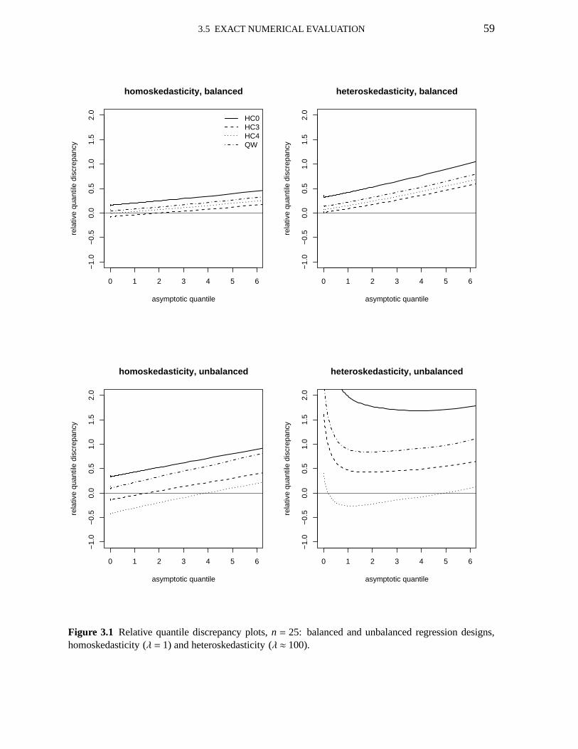
3.5 EXACT NUMERICAL EVALUATION 59
0 1 2 3 4 5 6
−1.
0−
0.5
0.0
0.5
1.0
1.5
2.0
asymptotic quantile
rela
tive
quan
tile
disc
repa
ncy
HC0HC3HC4QW
homoskedasticity, balanced
0 1 2 3 4 5 6
−1.
0−
0.5
0.0
0.5
1.0
1.5
2.0
asymptotic quantile
rela
tive
quan
tile
disc
repa
ncy
heteroskedasticity, balanced
0 1 2 3 4 5 6
−1.
0−
0.5
0.0
0.5
1.0
1.5
2.0
asymptotic quantile
rela
tive
quan
tile
disc
repa
ncy
homoskedasticity, unbalanced
0 1 2 3 4 5 6
−1.
0−
0.5
0.0
0.5
1.0
1.5
2.0
asymptotic quantile
rela
tive
quan
tile
disc
repa
ncy
heteroskedasticity, unbalanced
Figure 3.1 Relative quantile discrepancy plots,n = 25: balanced and unbalanced regression designs,homoskedasticity (λ = 1) and heteroskedasticity (λ ≈ 100).
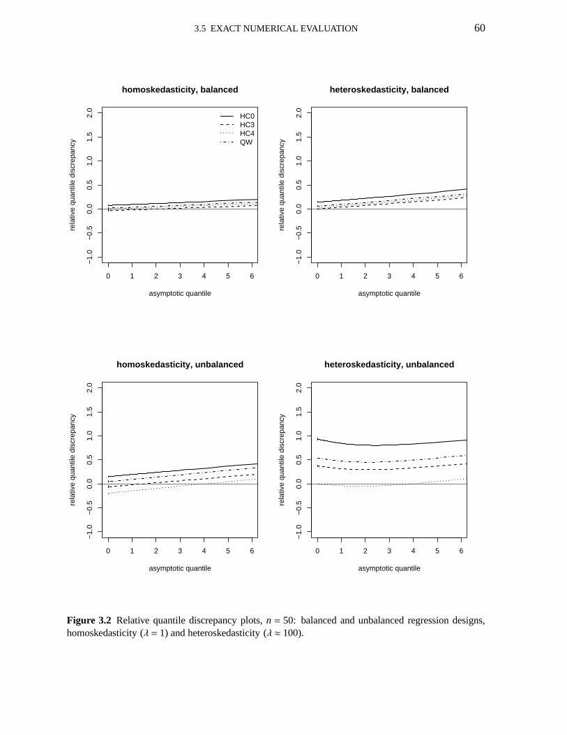
3.5 EXACT NUMERICAL EVALUATION 60
0 1 2 3 4 5 6
−1.
0−
0.5
0.0
0.5
1.0
1.5
2.0
asymptotic quantile
rela
tive
quan
tile
disc
repa
ncy
HC0HC3HC4QW
homoskedasticity, balanced
0 1 2 3 4 5 6
−1.
0−
0.5
0.0
0.5
1.0
1.5
2.0
asymptotic quantile
rela
tive
quan
tile
disc
repa
ncy
heteroskedasticity, balanced
0 1 2 3 4 5 6
−1.
0−
0.5
0.0
0.5
1.0
1.5
2.0
asymptotic quantile
rela
tive
quan
tile
disc
repa
ncy
homoskedasticity, unbalanced
0 1 2 3 4 5 6
−1.
0−
0.5
0.0
0.5
1.0
1.5
2.0
asymptotic quantile
rela
tive
quan
tile
disc
repa
ncy
heteroskedasticity, unbalanced
Figure 3.2 Relative quantile discrepancy plots,n = 50: balanced and unbalanced regression designs,homoskedasticity (λ = 1) and heteroskedasticity (λ ≈ 100).
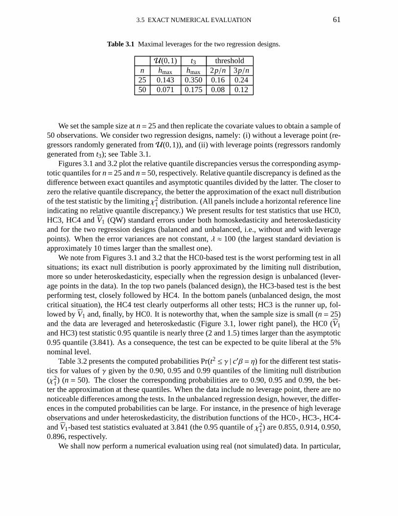
3.5 EXACT NUMERICAL EVALUATION 61
Table 3.1 Maximal leverages for the two regression designs.
U(0,1) t3 thresholdn hmax hmax 2p/n 3p/n25 0.143 0.350 0.16 0.2450 0.071 0.175 0.08 0.12
We set the sample size atn= 25 and then replicate the covariate values to obtain a sampleof50 observations. We consider two regression designs, namely: (i) without a leverage point (re-gressors randomly generated fromU(0,1)), and (ii) with leverage points (regressors randomlygenerated fromt3); see Table 3.1.
Figures 3.1 and 3.2 plot the relative quantile discrepancies versus the corresponding asymp-totic quantiles forn= 25 andn= 50, respectively. Relative quantile discrepancy is definedas thedifference between exact quantiles and asymptotic quantiles divided by the latter. The closer tozero the relative quantile discrepancy, the better the approximation of the exact null distributionof the test statistic by the limitingχ2
1 distribution. (All panels include a horizontal reference lineindicating no relative quantile discrepancy.) We present results for test statistics that use HC0,HC3, HC4 andV1 (QW) standard errors under both homoskedasticity and heteroskedasticityand for the two regression designs (balanced and unbalanced, i.e., without and with leveragepoints). When the error variances are not constant,λ ≈ 100 (the largest standard deviation isapproximately 10 times larger than the smallest one).
We note from Figures 3.1 and 3.2 that the HC0-based test is theworst performing test in allsituations; its exact null distribution is poorly approximated by the limiting null distribution,more so under heteroskedasticity, especially when the regression design is unbalanced (lever-age points in the data). In the top two panels (balanced design), the HC3-based test is the bestperforming test, closely followed by HC4. In the bottom panels (unbalanced design, the mostcritical situation), the HC4 test clearly outperforms all other tests; HC3 is the runner up, fol-lowed byV1 and, finally, by HC0. It is noteworthy that, when the sample size is small (n= 25)and the data are leveraged and heteroskedastic (Figure 3.1,lower right panel), the HC0 (V1
and HC3) test statistic 0.95 quantile is nearly three (2 and 1.5) times larger than the asymptotic0.95 quantile (3.841). As a consequence, the test can be expected to be quite liberal at the 5%nominal level.
Table 3.2 presents the computed probabilities Pr(t2 ≤ γ | c′β = η) for the different test statis-tics for values ofγ given by the 0.90, 0.95 and 0.99 quantiles of the limiting null distribution(χ2
1) (n = 50). The closer the corresponding probabilities are to 0.90, 0.95 and 0.99, the bet-ter the approximation at these quantiles. When the data include no leverage point, there are nonoticeable differences among the tests. In the unbalanced regression design, however, the differ-ences in the computed probabilities can be large. For instance, in the presence of high leverageobservations and under heteroskedasticity, the distribution functions of the HC0-, HC3-, HC4-andV1-based test statistics evaluated at 3.841 (the 0.95 quantile ofχ2
1) are 0.855, 0.914, 0.950,0.896, respectively.
We shall now perform a numerical evaluation using real (not simulated) data. In particular,
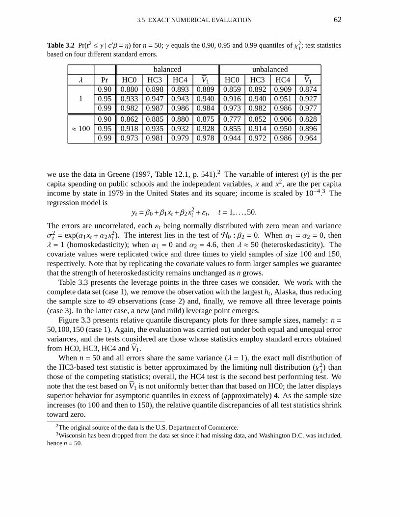
3.5 EXACT NUMERICAL EVALUATION 62
Table 3.2 Pr(t2 ≤ γ | c′β = η) for n= 50; γ equals the 0.90, 0.95 and 0.99 quantiles ofχ21; test statistics
based on four different standard errors.
balanced unbalancedλ Pr HC0 HC3 HC4 V1 HC0 HC3 HC4 V1
0.90 0.880 0.898 0.893 0.889 0.859 0.892 0.909 0.8741 0.95 0.933 0.947 0.943 0.940 0.916 0.940 0.951 0.927
0.99 0.982 0.987 0.986 0.984 0.973 0.982 0.986 0.977
0.90 0.862 0.885 0.880 0.875 0.777 0.852 0.906 0.828≈ 100 0.95 0.918 0.935 0.932 0.928 0.855 0.914 0.950 0.896
0.99 0.973 0.981 0.979 0.978 0.944 0.972 0.986 0.964
we use the data in Greene (1997, Table 12.1, p. 541).2 The variable of interest (y) is the percapita spending on public schools and the independent variables,x andx2, are the per capitaincome by state in 1979 in the United States and its square; income is scaled by 10−4.3 Theregression model is
yt = β0+β1xt +β2x2t +εt, t = 1, . . . ,50.
The errors are uncorrelated, eachεt being normally distributed with zero mean and varianceσ2
t = exp(α1xt +α2x2t ). The interest lies in the test ofH0 : β2 = 0. Whenα1 = α2 = 0, then
λ = 1 (homoskedasticity); whenα1 = 0 andα2 = 4.6, thenλ ≈ 50 (heteroskedasticity). Thecovariate values were replicated twice and three times to yield samples of size 100 and 150,respectively. Note that by replicating the covariate values to form larger samples we guaranteethat the strength of heteroskedasticity remains unchangedasn grows.
Table 3.3 presents the leverage points in the three cases we consider. We work with thecomplete data set (case 1), we remove the observation with the largestht, Alaska, thus reducingthe sample size to 49 observations (case 2) and, finally, we remove all three leverage points(case 3). In the latter case, a new (and mild) leverage point emerges.
Figure 3.3 presents relative quantile discrepancy plots for three sample sizes, namely:n=50,100,150 (case 1). Again, the evaluation was carried out under both equal and unequal errorvariances, and the tests considered are those whose statistics employ standard errors obtainedfrom HC0, HC3, HC4 andV1.
Whenn = 50 and all errors share the same variance (λ = 1), the exact null distribution ofthe HC3-based test statistic is better approximated by the limiting null distribution (χ2
1) thanthose of the competing statistics; overall, the HC4 test is the second best performing test. Wenote that the test based onV1 is not uniformly better than that based on HC0; the latter displayssuperior behavior for asymptotic quantiles in excess of (approximately) 4. As the sample sizeincreases (to 100 and then to 150), the relative quantile discrepancies of all test statistics shrinktoward zero.
2The original source of the data is the U.S. Department of Commerce.3Wisconsin has been dropped from the data set since it had missing data, and Washington D.C. was included,
hencen= 50.
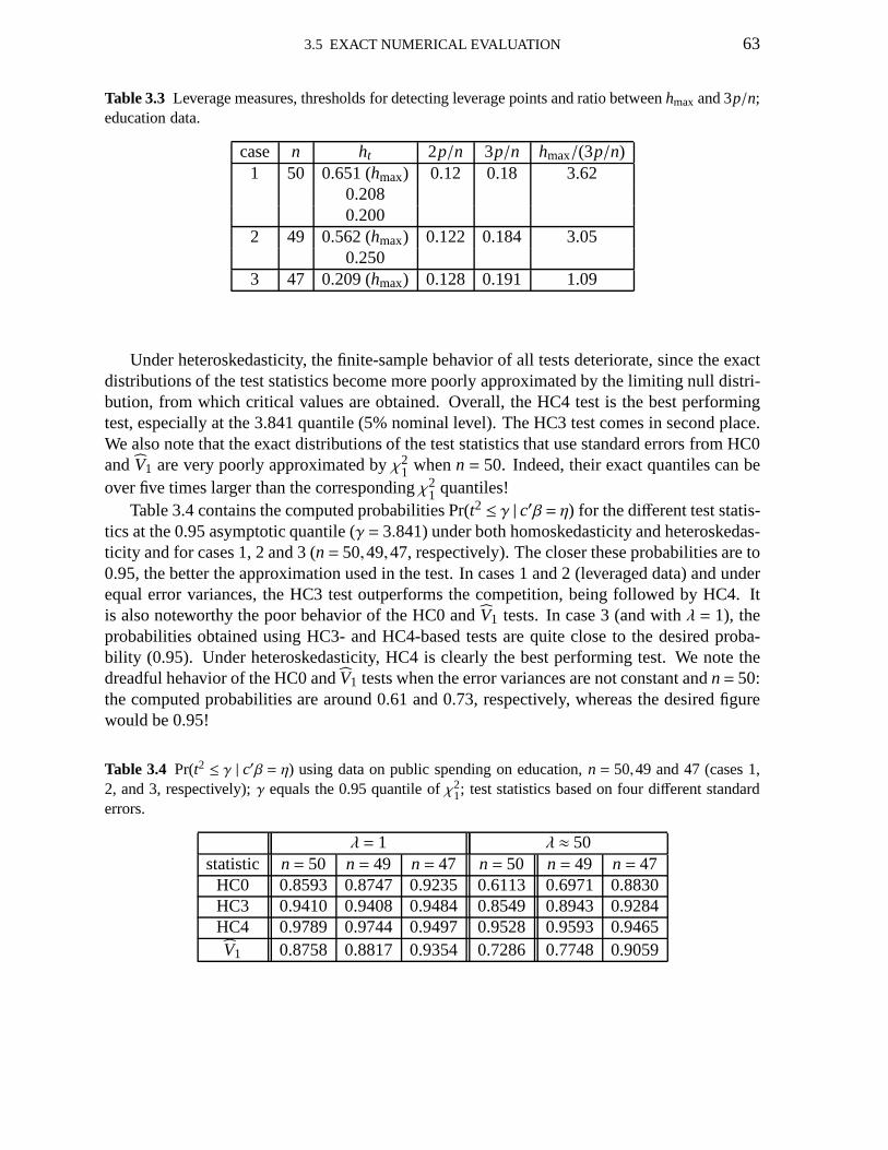
3.5 EXACT NUMERICAL EVALUATION 63
Table 3.3 Leverage measures, thresholds for detecting leverage points and ratio betweenhmax and 3p/n;education data.
case n ht 2p/n 3p/n hmax/(3p/n)1 50 0.651 (hmax) 0.12 0.18 3.62
0.2080.200
2 49 0.562 (hmax) 0.122 0.184 3.050.250
3 47 0.209 (hmax) 0.128 0.191 1.09
Under heteroskedasticity, the finite-sample behavior of all tests deteriorate, since the exactdistributions of the test statistics become more poorly approximated by the limiting null distri-bution, from which critical values are obtained. Overall, the HC4 test is the best performingtest, especially at the 3.841 quantile (5% nominal level). The HC3 test comes in second place.We also note that the exact distributions of the test statistics that use standard errors from HC0andV1 are very poorly approximated byχ2
1 whenn= 50. Indeed, their exact quantiles can beover five times larger than the correspondingχ2
1 quantiles!Table 3.4 contains the computed probabilities Pr(t2 ≤ γ | c′β = η) for the different test statis-
tics at the 0.95 asymptotic quantile (γ = 3.841) under both homoskedasticity and heteroskedas-ticity and for cases 1, 2 and 3 (n= 50,49,47, respectively). The closer these probabilities are to0.95, the better the approximation used in the test. In cases1 and 2 (leveraged data) and underequal error variances, the HC3 test outperforms the competition, being followed by HC4. Itis also noteworthy the poor behavior of the HC0 andV1 tests. In case 3 (and withλ = 1), theprobabilities obtained using HC3- and HC4-based tests are quite close to the desired proba-bility (0.95). Under heteroskedasticity, HC4 is clearly the best performing test. We note thedreadful hehavior of the HC0 andV1 tests when the error variances are not constant andn= 50:the computed probabilities are around 0.61 and 0.73, respectively, whereas the desired figurewould be 0.95!
Table 3.4 Pr(t2 ≤ γ | c′β = η) using data on public spending on education,n = 50,49 and 47 (cases 1,2, and 3, respectively);γ equals the 0.95 quantile ofχ2
1; test statistics based on four different standarderrors.
λ = 1 λ ≈ 50statistic n= 50 n= 49 n= 47 n= 50 n= 49 n= 47
HC0 0.8593 0.8747 0.9235 0.6113 0.6971 0.8830HC3 0.9410 0.9408 0.9484 0.8549 0.8943 0.9284HC4 0.9789 0.9744 0.9497 0.9528 0.9593 0.9465V1 0.8758 0.8817 0.9354 0.7286 0.7748 0.9059
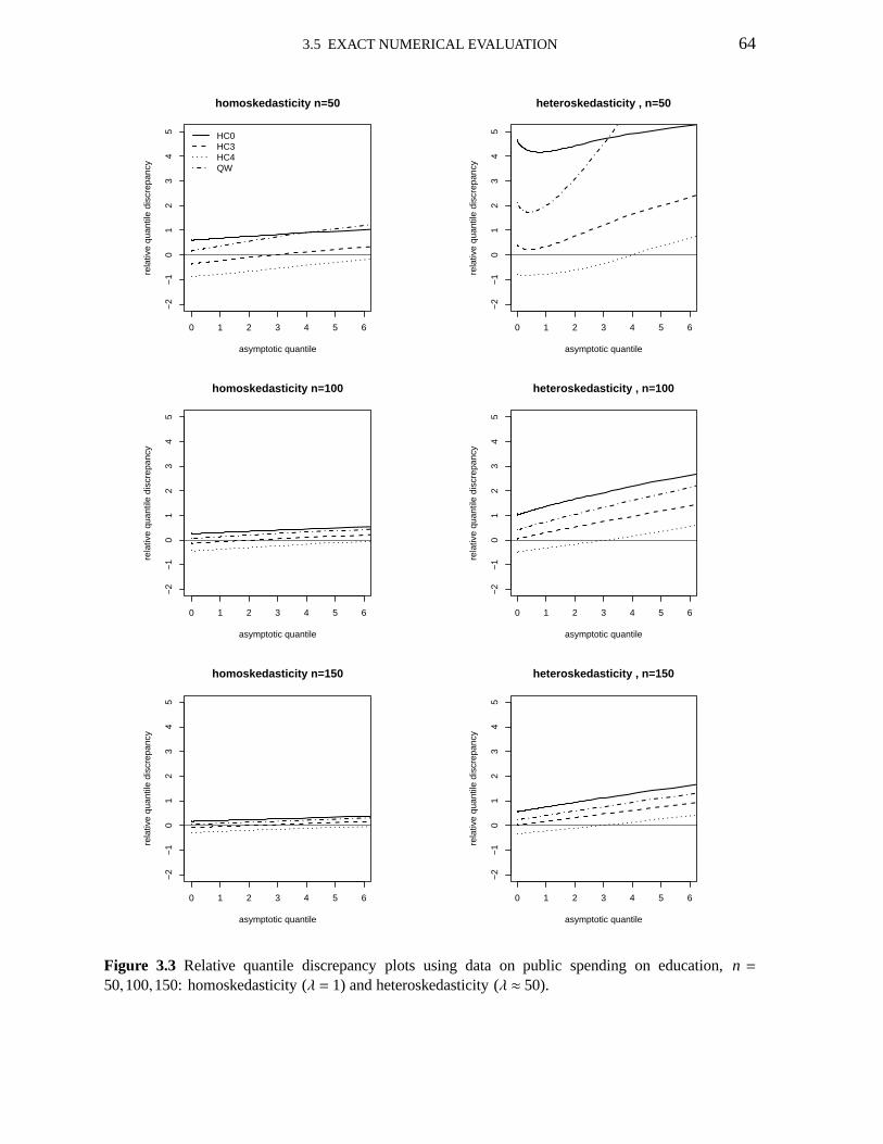
3.5 EXACT NUMERICAL EVALUATION 64
0 1 2 3 4 5 6
−2
−1
01
23
45
asymptotic quantile
rela
tive
quan
tile
disc
repa
ncy
HC0HC3HC4QW
homoskedasticity n=50
0 1 2 3 4 5 6
−2
−1
01
23
45
asymptotic quantile
rela
tive
quan
tile
disc
repa
ncy
heteroskedasticity , n=50
0 1 2 3 4 5 6
−2
−1
01
23
45
asymptotic quantile
rela
tive
quan
tile
disc
repa
ncy
homoskedasticity n=100
0 1 2 3 4 5 6
−2
−1
01
23
45
asymptotic quantile
rela
tive
quan
tile
disc
repa
ncy
heteroskedasticity , n=100
0 1 2 3 4 5 6
−2
−1
01
23
45
asymptotic quantile
rela
tive
quan
tile
disc
repa
ncy
homoskedasticity n=150
0 1 2 3 4 5 6
−2
−1
01
23
45
asymptotic quantile
rela
tive
quan
tile
disc
repa
ncy
heteroskedasticity , n=150
Figure 3.3 Relative quantile discrepancy plots using data on public spending on education,n =50,100,150: homoskedasticity (λ = 1) and heteroskedasticity (λ ≈ 50).

3.6 AN ALTERNATIVE STANDARD ERROR 65
3.6 An alternative standard error
Qian and Wang (2001) have proposed an additional alternative HCCME, which we shall denoteasV2. It is given byV2 = PD2P′, where
D2 = diagd2t = diagε2t + σ2ht = Ω+ σ2(H)d = Ω+ σ2K;
as before,K = (H)d, i.e.,K is obtained by setting all nondiagonal elements ofH (the hat matrix)equal to zero.
We will show that, like their other estimator (V1), this HCCME is unbiased under equalerror variances. It follows from (3.2.1) that
E[ε] = E[My] = E[M(Xβ+ε)] = E[Mε] = 0,
sinceMX = (I −H)X = 0. Given thatΩ = diagε2t = (εε′)d, and that
E[ εε′] = cov(ε)+E[ε]E[ε′]
= cov(Mε)
= MΩM,
we haveE[Ω] = E[(εε′)d] = (I −H)Ω(I −H)d.
Note that
E[Ω] = (I −H)Ω(I −H)d = HΩH −2HΩ+Ωd = HΩ(H −2I )d+Ω = M(1)(Ω)+Ω,
whereM(1)(Ω) = HΩ(H −2I )d. Under homoskedasticity,
E[Ω] = M(1)(σ2I )+σ2I
= Hσ2I (H −2I )d+σ2I
= σ2HH −2Hd+σ2I
= σ2−Hd+σ2I
= −σ2K +σ2I
= σ2(I −K).
Using the definition ofD2, it follows that
E[D2] = E[Ω] +E[σ2]K
= σ2(I −K)+σ2K
= σ2I .
Thus, when all errors share the same variance,
V2 = PD2P′
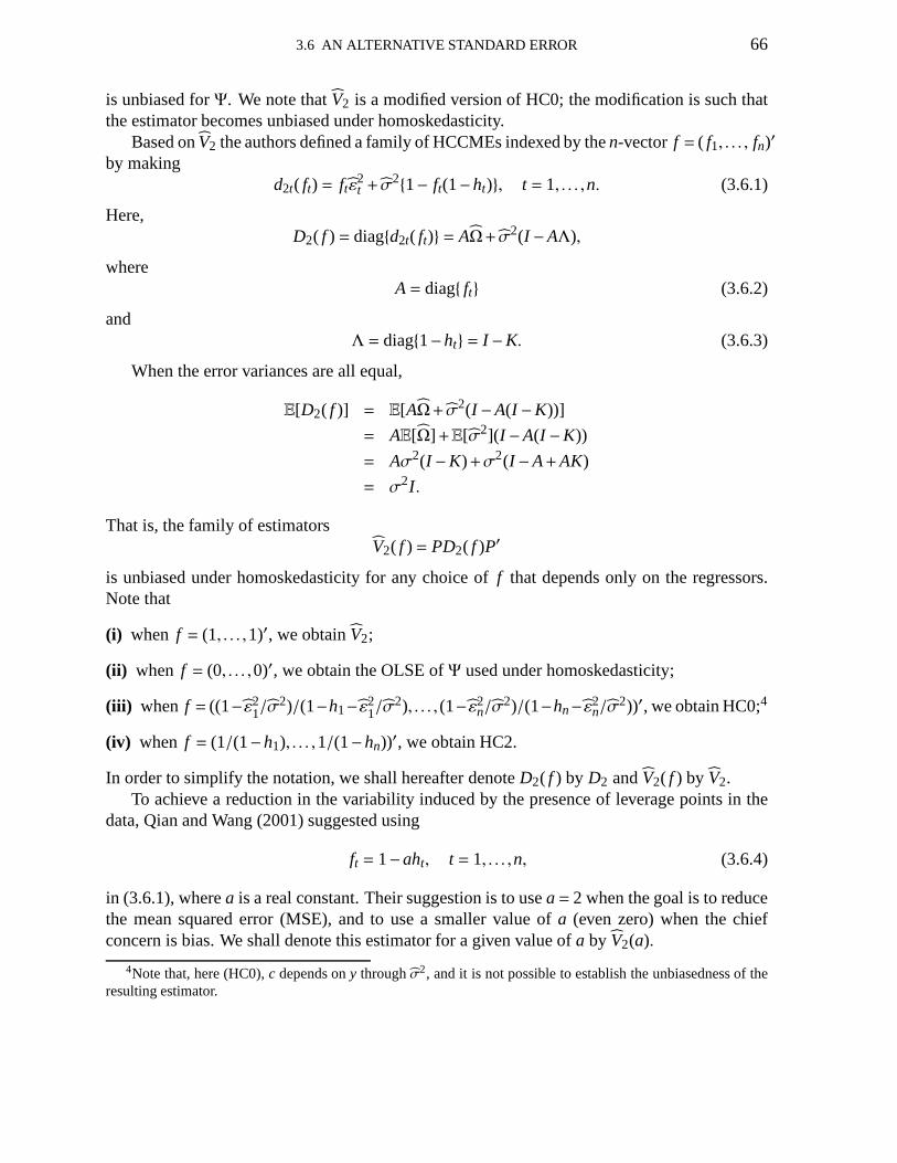
3.6 AN ALTERNATIVE STANDARD ERROR 66
is unbiased forΨ. We note thatV2 is a modified version of HC0; the modification is such thatthe estimator becomes unbiased under homoskedasticity.
Based onV2 the authors defined a family of HCCMEs indexed by then-vector f = ( f1, . . . , fn)′
by makingd2t( ft) = ftε
2t + σ
21− ft(1−ht), t = 1, . . . ,n. (3.6.1)
Here,D2( f ) = diagd2t( ft) = AΩ+ σ2(I −AΛ),
whereA= diag ft (3.6.2)
andΛ = diag1−ht = I −K. (3.6.3)
When the error variances are all equal,
E[D2( f )] = E[AΩ+ σ2(I −A(I −K))]
= AE[Ω] +E[σ2](I −A(I −K))
= Aσ2(I −K)+σ2(I −A+AK)
= σ2I .
That is, the family of estimatorsV2( f ) = PD2( f )P′
is unbiased under homoskedasticity for any choice off that depends only on the regressors.Note that
(i) when f = (1, . . . ,1)′, we obtainV2;
(ii) when f = (0, . . . ,0)′, we obtain the OLSE ofΨ used under homoskedasticity;
(iii) when f = ((1− ε21/σ2)/(1−h1− ε21/σ
2), . . . , (1− ε2n/σ2)/(1−hn− ε2n/σ2))′, we obtain HC0;4
(iv) when f = (1/(1−h1), . . . ,1/(1−hn))′, we obtain HC2.
In order to simplify the notation, we shall hereafter denoteD2( f ) by D2 andV2( f ) by V2.To achieve a reduction in the variability induced by the presence of leverage points in the
data, Qian and Wang (2001) suggested using
ft = 1−aht, t = 1, . . . ,n, (3.6.4)
in (3.6.1), wherea is a real constant. Their suggestion is to usea= 2 when the goal is to reducethe mean squared error (MSE), and to use a smaller value ofa (even zero) when the chiefconcern is bias. We shall denote this estimator for a given value ofa by V2(a).
4Note that, here (HC0),c depends ony throughσ2, and it is not possible to establish the unbiasedness of theresulting estimator.

3.6 AN ALTERNATIVE STANDARD ERROR 67
In Section 3.3 we have shown that the estimator ofΦ, the variance ofc′β, that usesV1 isgiven byΦQW1 = ε
′[W−M(1)(W)]ε = ε′VQW1ε, whereVQW1 =W−M(1)(W). By writing ΦQW1
as a quadratic form in a vector of uncorrelated, zero mean andunit variance random variableswe obtainedΦQW1 = z′GQW1z, whereE[z] = 0, cov(z) = I and
GQW1 = Ω1/2(I −H)VQW1(I −H)Ω1/2.
WhenV2 = ΨQW2 = PD2P′ is used in the estimation ofΦ, we obtain
ΦQW2 = c′ΨQW2c= c′PD2P′c,
whereD2 = AΩ+ σ2(I −AΛ); A andΛ are as defined in (3.6.2) and (3.6.3), respectively.Let L = (n− p)−1(I −AΛ). Then,5
D2 = ε′εL+AΩ.
Let ℓ = L1/2P′c, v∗ = A1/2P′c andV∗ = (v∗v∗′)d. Note that
v∗′Ωv∗ = v∗
′[( εε′)d]v∗ = ε′[(v∗v∗
′)d]ε = ε′V∗ε
andℓ′(ε′εI )ℓ = ε′[ℓ′ℓI ]ε.
Therefore,
ΦQW2 = c′PD2P′c
= c′P[ε′εL+AΩ]P′c
= c′P[L1/2(ε′εI )L1/2+A1/2ΩA1/2]P′c
= c′PL1/2(ε′εI )L1/2P′c+c′PA1/2ΩA1/2P′c
= ℓ′(ε′εI )ℓ+v∗′Ωv∗
= ε′(ℓ′ℓI )ε+ ε′V∗ε
= ε′(ℓ′ℓI +V∗)ε
= ε′VQW2ε,
whereVQW2 = ℓ′ℓI +V∗.
We then writeΦQW2 as a quadratic form in a vector of uncorrelated, zero mean andunitvariance random variables (z) as
ΦQW2 = z′GQW2z,
whereGQW2 = Ω
1/2(I −H)VQW2(I −H)Ω1/2.
5Recall thatσ2 = (n− p)−1ε′ε.
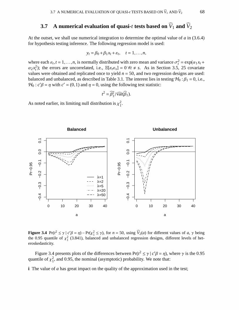
3.7 A NUMERICAL EVALUATION OF QUASI-t TESTS BASED ONV1 AND V2 68
3.7 A numerical evaluation of quasi-t tests based onV1 and V2
At the outset, we shall use numerical integration to determine the optimal value ofa in (3.6.4)for hypothesis testing inference. The following regression model is used:
yt = β0+β1xt +εt, t = 1, . . . ,n,
where eachεt, t = 1, . . . ,n, is normally distributed with zero mean and varianceσ2t = exp(α1xt+
α2x2t ); the errors are uncorrelated, i.e.,E[εtεs] = 0∀t , s. As in Section 3.5, 25 covariate
values were obtained and replicated once to yieldn= 50, and two regression designs are used:balanced and unbalanced, as described in Table 3.1. The interest lies in testingH0 : β1 = 0, i.e.,H0 : c′β = η with c′ = (0,1) andη = 0, using the following test statistic:
t2 = β21/var(β1).
As noted earlier, its limiting null distribution isχ21.
0 10 20 30 40
−0.
4−
0.3
−0.
2−
0.1
0.0
0.1
a
Pr−
0.95
λ=1λ=2λ=5λ=20λ=50
Balanced
0 10 20 30 40
−0.
4−
0.3
−0.
2−
0.1
0.0
0.1
a
Pr−
0.95
Unbalanced
Figure 3.4 Pr(t2 ≤ γ | c′β = η)−Pr(χ21 ≤ γ), for n = 50, usingV2(a) for different values ofa, γ being
the 0.95 quantile ofχ21 (3.841), balanced and unbalanced regression designs, different levels of het-
eroskedasticity.
Figure 3.4 presents plots of the differences between Pr(t2 ≤ γ | c′β = η), whereγ is the 0.95quantile ofχ2
1, and 0.95, the nominal (asymptotic) probability. We note that:
i The value ofa has great impact on the quality of the approximation used in the test;
3.7 A NUMERICAL EVALUATION OF QUASI-t TESTS BASED ONV1 AND V2 69
ii The optimal value ofa depends on the heteroskedasticity strength and also on whether thedata contain high leverage observations;
iii The differences of the two probabilities (exact and asymptotic) arenot monotonic ina;
iv In balanced regression designs it is best to usea = 0, whereas under leveraged data oneshould usea≈ 15.
v In the presence of high leverage observations, the optimal value ofa for hypothesis testinginference is quite different from that proposed by Qian and Wang (2001).6
Figure 3.5 contains relative quantile discrepancies plotsfor test statistics based onV1 andV2(a) for a= 0,2,10,15. We note from Figure 3.5 that:
i The null distributions of all test statistics are well approximated by the limiting null distribu-tion (χ2
1) when all errors share the same variance and the regression design is balanced;
ii In the absence of leverage points and under heteroskedasticity, the null distributions of thetest statistics based on the following HCCMEs are well approximated by the limiting nulldistribution (χ2
1): V1, V2(0) andV2(2);
iii Under homoskedasticity and leveraged data, the quantiles of the test statistics based onV1,V2(0) andV2(2) are similar;
iv Under heteroskedasticity and leveraged data, the best performing test is that based onV2(a)with a= 15, which is clearly superior to the alternative tests.
Table 3.5 presents the computed probabilities Pr(t2 ≤ γ | c′β = η) at the 0.90, 0.95 and 0.99asymptotic (χ2
1) quantiles for test statistics based on HC3, HC4,V1 andV2(a) with a= 0,2 e 15whenλ = 1, λ ≈ 50 andλ ≈ 100. The figures in this table suggest that:
i Under homoskedasticity and balanced data, all probabilitydiscrepancies are small, i.e., thecomputed exact probabilities are close to their nominal counterparts (0.90, 0.95 and0.99);
ii When the errors have different variances and the regression design is balanced (no leveragepoint), the following estimators yield exact probabilities that are close to the respectiveasymptotic probabilities: HC3, HC4,V1 and V2(a) with a = 0 anda = 2 (with slightadvantage to HC3 and HC4);
iii When the error variances are constant and the data are leveraged, the only estimator thatyields exact probabilities that are not close to the asymptotic ones isV2(15), the smallestprobability discrepancies being those of HC4;
6Recall that these authors proposed usinga= 2 for MSE minimization.
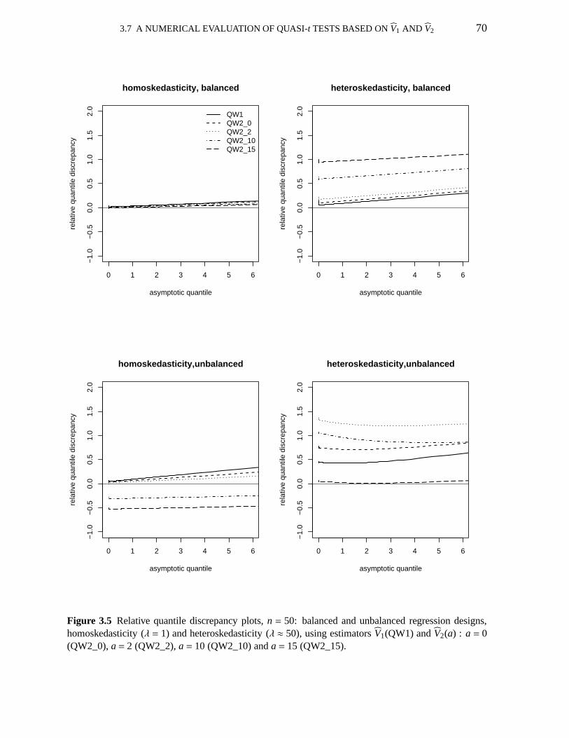
3.7 A NUMERICAL EVALUATION OF QUASI-t TESTS BASED ONV1 AND V2 70
0 1 2 3 4 5 6
−1.
0−
0.5
0.0
0.5
1.0
1.5
2.0
asymptotic quantile
rela
tive
quan
tile
disc
repa
ncy
QW1QW2_0QW2_2QW2_10QW2_15
homoskedasticity, balanced
0 1 2 3 4 5 6
−1.
0−
0.5
0.0
0.5
1.0
1.5
2.0
asymptotic quantilere
lativ
e qu
antil
e di
scre
panc
y
heteroskedasticity, balanced
0 1 2 3 4 5 6
−1.
0−
0.5
0.0
0.5
1.0
1.5
2.0
asymptotic quantile
rela
tive
quan
tile
disc
repa
ncy
homoskedasticity,unbalanced
0 1 2 3 4 5 6
−1.
0−
0.5
0.0
0.5
1.0
1.5
2.0
asymptotic quantile
rela
tive
quan
tile
disc
repa
ncy
heteroskedasticity,unbalanced
Figure 3.5 Relative quantile discrepancy plots,n = 50: balanced and unbalanced regression designs,homoskedasticity (λ = 1) and heteroskedasticity (λ ≈ 50), using estimatorsV1(QW1) andV2(a) : a = 0(QW2_0),a= 2 (QW2_2),a= 10 (QW2_10) anda= 15 (QW2_15).
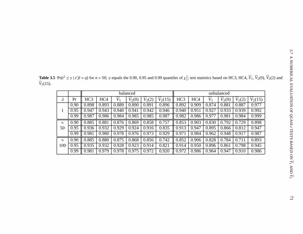
3.7
AN
UM
ER
ICA
LE
VAL
UA
TIO
NO
FQ
UA
SI-tT
ES
TS
BA
SE
DO
NV1
AN
DV
27
1
Table 3.5 Pr(t2 ≤ γ | c′β = η) for n= 50; γ equals the 0.90, 0.95 and 0.99 quantiles ofχ21; test statistics based on HC3, HC4,V1, V2(0), V2(2) and
V2(15).
balanced unbalancedλ Pr HC3 HC4 V1 V2(0) V2(2) V2(15) HC3 HC4 V1 V2(0) V2(2) V2(15)
0.90 0.898 0.893 0.889 0.890 0.891 0.896 0.892 0.909 0.874 0.881 0.887 0.9771 0.95 0.947 0.943 0.940 0.941 0.942 0.946 0.940 0.951 0.927 0.933 0.939 0.992
0.99 0.987 0.986 0.984 0.985 0.985 0.987 0.982 0.986 0.977 0.981 0.984 0.999
≈ 0.90 0.885 0.881 0.876 0.869 0.858 0.757 0.853 0.903 0.830 0.792 0.729 0.89850 0.95 0.936 0.932 0.929 0.924 0.916 0.835 0.913 0.947 0.895 0.866 0.812 0.947
0.99 0.981 0.980 0.978 0.976 0.973 0.929 0.971 0.984 0.962 0.948 0.917 0.987
≈ 0.90 0.885 0.880 0.875 0.868 0.856 0.742 0.852 0.906 0.828 0.784 0.711 0.893100 0.95 0.935 0.932 0.928 0.923 0.914 0.821 0.914 0.950 0.896 0.861 0.798 0.945
0.99 0.981 0.979 0.978 0.975 0.972 0.920 0.972 0.986 0.964 0.947 0.910 0.986

3.8 YET ANOTHER HETEROSKEDASTICITY-CONSISTENT STANDARD ERROR: HC5 72
iv Under heteroskedasticity and leveraged data, the estimators HC4 andV2(15) yield the bestperforming tests, i.e., the exact probabilities of the teststatistics that use HC4 andV2(15)variance estimates are considerably closer to their nominal counterparts than those asso-ciated with the competing test statistics.
We now move to a second numerical evaluation, which uses the data on public spending oneducation described earlier. The model used in the numerical exercise was
yt = β0+β1xt +β2x2t +εt, t = 1, . . . ,50,
the skedastic function being as described in Section 3.5. Wehave used numerical integrationto compute the exact quantiles of the following test statistics: HC3, HC4,V1 andV2(a) witha = 0,2,15. The sample sizes weren = 50,100 and computations were carried under bothhomoskedasticity (λ = 1) and heteroskedasticity (λ ≈ 50).
We note from Figure 3.6, which contains the relevant quantile discrepancy plots, that underequal error variances the smallest relative quantile discrepancies are those of the test statisticsbased onV2(0) andV2(2). Under heteroskedasticity, however, the best performing tests areV2(15) e HC4.
3.8 Yet another heteroskedasticity-consistent standard error: HC5
In Section 3.2, we presented four HCCMEs in which thetth squared residual is divided by(1− ht)δt ; δt = 0 for HC0, δt = 1 for HC2, δt = 2 for HC3 andδt = min4,nht/p for HC4.These adjustments aim at ‘inflating’ the squared residuals according to their respective leveragemeasures, which are obtained from the hat matrix.
Cribari–Neto, Souza and Vasconcellos (2007) have proposedthe HC5 estimator, which isgiven by
HC5= PΩ5P′ = PE5ΩP′,
whereE5 = diag1/√
(1−ht)δt and
δt =min
nht
p,max
4,
nkhmax
p
,
with hmax=maxh1, . . . ,hn. Here, 0< k < 1 is a constant; the authors suggested usingk = 0.7based on pilot Monte Carlo simulation results. It is noteworthy thathmax may now affect thediscount terms of all squared residuals, and not only of the corresponding squared residual.
We note that HC5 can also be used in the variance estimation ofa linear combination of theregression parameter estimates inβ. Here,
Φ5 = ε′V5ε,
whereV5 = (v5v′5)d andv5 = E1/25 P′c. It is possible to writeΦ5 as a quadratic form in a vector
z of zero mean and unit covariance asΦ5 = z′G5z, whereG5 = Ω1/2(I −H)V5(I −H)Ω1/2.
We shall now use Imhof’s (1961) numerical integration algorithm to obtain the exact nulldistributions of HC5-based test statistics and evaluate the first orderχ2
1 approximation used in
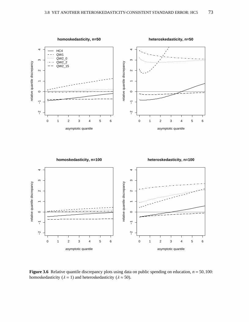
3.8 YET ANOTHER HETEROSKEDASTICITY-CONSISTENT STANDARD ERROR: HC5 73
0 1 2 3 4 5 6
−2
−1
01
23
4
asymptotic quantile
rela
tive
quan
tile
disc
repa
ncy
HC4QW1QW2_0QW2_2QW2_15
homoskedasticity, n=50
0 1 2 3 4 5 6
−2
−1
01
23
4asymptotic quantile
rela
tive
quan
tile
disc
repa
ncy
heteroskedasticity, n=50
0 1 2 3 4 5 6
−2
−1
01
23
4
asymptotic quantile
rela
tive
quan
tile
disc
repa
ncy
homoskedasticity, n=100
0 1 2 3 4 5 6
−2
−1
01
23
4
asymptotic quantile
rela
tive
quan
tile
disc
repa
ncy
heteroskedasticity, n=100
Figure 3.6 Relative quantile discrepancy plots using data on public spending on education,n= 50,100:homoskedasticity (λ = 1) and heteroskedasticity (λ ≈ 50).
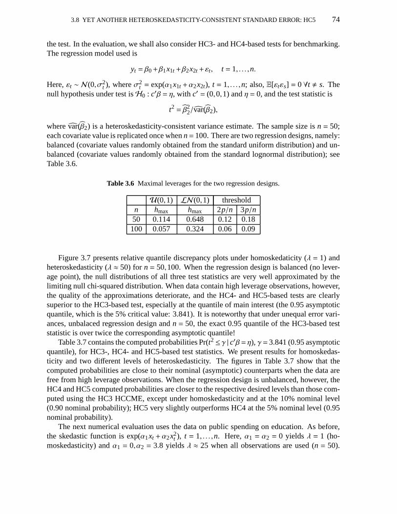
3.8 YET ANOTHER HETEROSKEDASTICITY-CONSISTENT STANDARD ERROR: HC5 74
the test. In the evaluation, we shall also consider HC3- and HC4-based tests for benchmarking.The regression model used is
yt = β0+β1x1t +β2x2t +εt, t = 1, . . . ,n.
Here,εt ∼ N(0,σ2t ), whereσ2
t = exp(α1x1t +α2x2t), t = 1, . . . ,n; also,E[εtεs] = 0∀t , s. Thenull hypothesis under test isH0 : c′β = η, with c′ = (0,0,1) andη = 0, and the test statistic is
t2 = β22/var(β2),
wherevar(β2) is a heteroskedasticity-consistent variance estimate. The sample size isn = 50;each covariate value is replicated once whenn= 100. There are two regression designs, namely:balanced (covariate values randomly obtained from the standard uniform distribution) and un-balanced (covariate values randomly obtained from the standard lognormal distribution); seeTable 3.6.
Table 3.6 Maximal leverages for the two regression designs.
U(0,1) LN(0,1) thresholdn hmax hmax 2p/n 3p/n50 0.114 0.648 0.12 0.18100 0.057 0.324 0.06 0.09
Figure 3.7 presents relative quantile discrepancy plots under homoskedaticity (λ = 1) andheteroskedasticity (λ ≈ 50) for n= 50,100. When the regression design is balanced (no lever-age point), the null distributions of all three test statistics are very well approximated by thelimiting null chi-squared distribution. When data containhigh leverage observations, however,the quality of the approximations deteriorate, and the HC4-and HC5-based tests are clearlysuperior to the HC3-based test, especially at the quantile of main interest (the 0.95 asymptoticquantile, which is the 5% critical value: 3.841). It is noteworthy that under unequal error vari-ances, unbalaced regression design andn = 50, the exact 0.95 quantile of the HC3-based teststatistic is over twice the corresponding asymptotic quantile!
Table 3.7 contains the computed probabilities Pr(t2≤ γ | c′β= η), γ= 3.841 (0.95 asymptoticquantile), for HC3-, HC4- and HC5-based test statistics. Wepresent results for homoskedas-ticity and two different levels of heteroskedasticity. The figures in Table 3.7show that thecomputed probabilities are close to their nominal (asymptotic) counterparts when the data arefree from high leverage observations. When the regression design is unbalanced, however, theHC4 and HC5 computed probabilities are closer to the respective desired levels than those com-puted using the HC3 HCCME, except under homoskedasticity and at the 10% nominal level(0.90 nominal probability); HC5 very slightly outperformsHC4 at the 5% nominal level (0.95nominal probability).
The next numerical evaluation uses the data on public spending on education. As before,the skedastic function is exp(α1xt +α2x2
t ), t = 1, . . . ,n. Here,α1 = α2 = 0 yieldsλ = 1 (ho-moskedasticity) andα1 = 0,α2 = 3.8 yieldsλ ≈ 25 when all observations are used (n = 50).
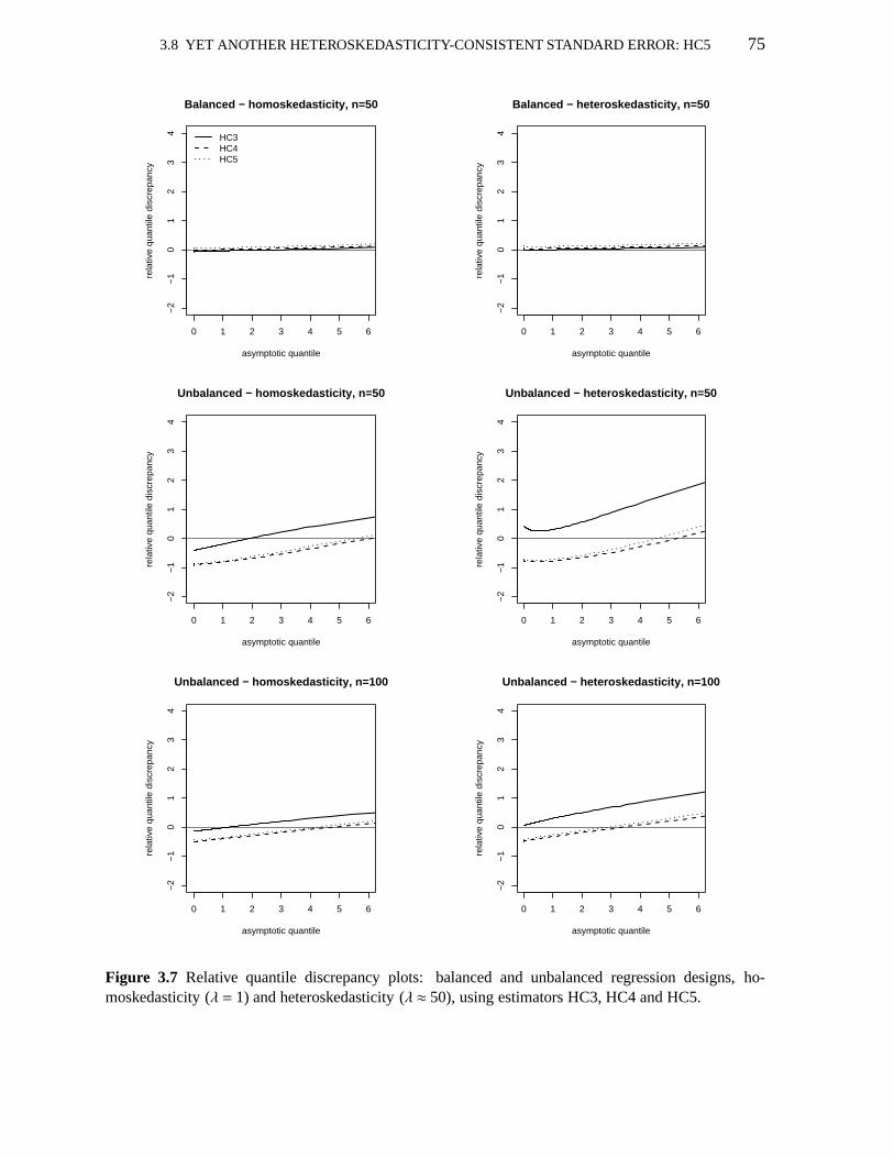
3.8 YET ANOTHER HETEROSKEDASTICITY-CONSISTENT STANDARD ERROR: HC5 75
0 1 2 3 4 5 6
−2
−1
01
23
4
asymptotic quantile
rela
tive
quan
tile
disc
repa
ncy
HC3HC4HC5
Balanced − homoskedasticity, n=50
0 1 2 3 4 5 6
−2
−1
01
23
4
asymptotic quantile
rela
tive
quan
tile
disc
repa
ncy
Balanced − heteroskedasticity, n=50
0 1 2 3 4 5 6
−2
−1
01
23
4
asymptotic quantile
rela
tive
quan
tile
disc
repa
ncy
Unbalanced − homoskedasticity, n=50
0 1 2 3 4 5 6
−2
−1
01
23
4
asymptotic quantile
rela
tive
quan
tile
disc
repa
ncy
Unbalanced − heteroskedasticity, n=50
0 1 2 3 4 5 6
−2
−1
01
23
4
asymptotic quantile
rela
tive
quan
tile
disc
repa
ncy
Unbalanced − homoskedasticity, n=100
0 1 2 3 4 5 6
−2
−1
01
23
4
asymptotic quantile
rela
tive
quan
tile
disc
repa
ncy
Unbalanced − heteroskedasticity, n=100
Figure 3.7 Relative quantile discrepancy plots: balanced and unbalanced regression designs, ho-moskedasticity (λ = 1) and heteroskedasticity (λ ≈ 50), using estimators HC3, HC4 and HC5.
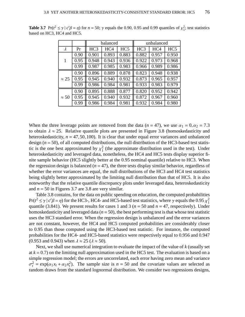
3.8 YET ANOTHER HETEROSKEDASTICITY-CONSISTENT STANDARD ERROR: HC5 76
Table 3.7 Pr(t2 ≤ γ | c′β = η) for n= 50; γ equals the 0.90, 0.95 and 0.99 quantiles ofχ21; test statistics
based on HC3, HC4 and HC5.
balanced unbalancedλ Pr HC3 HC4 HC5 HC3 HC4 HC5
0.90 0.901 0.893 0.883 0.882 0.957 0.9501 0.95 0.948 0.943 0.936 0.922 0.973 0.968
0.99 0.987 0.985 0.983 0.966 0.989 0.986
0.90 0.896 0.889 0.878 0.823 0.948 0.938≈ 25 0.95 0.945 0.940 0.932 0.873 0.965 0.957
0.99 0.986 0.984 0.981 0.933 0.983 0.979
0.90 0.895 0.888 0.877 0.820 0.952 0.942≈ 50 0.95 0.945 0.940 0.932 0.872 0.967 0.960
0.99 0.986 0.984 0.981 0.932 0.984 0.980
When the three leverage points are removed from the data (n = 47), we useα1 = 0,α2 = 7.3to obtainλ ≈ 25. Relative quantile plots are presented in Figure 3.8 (homoskedasticity andheteroskedasticity,n= 47,50,100). It is clear that under equal error variances and unbalanceddesign (n= 50), of all computed distributions, the null distribution of the HC3-based test statis-tic is the one best approximated byχ2
1 (the approximate distribution used in the test). Underheteroskedasticity and leveraged data, nonetheless, the HC4 and HC5 tests display superior fi-nite sample behavior (HC5 slightly better at the 0.95 nominal quantile) relative to HC3. Whenthe regression design is balanced (n= 47), the three tests display similar behavior, regardless ofwhether the error variances are equal, the null distributions of the HC3 and HC4 test statisticsbeing slightly better approximated by the limiting null distribution than that of HC5. It is alsonoteworthy that the relative quantile discrepancy plots under leveraged data, heteroskedasticityandn= 50 in Figures 3.7 are 3.8 are very similar.
Table 3.8 contains, for the data on public spending on education, the computed probabilitiesPr(t2≤ γ | c′β= η) for the HC3-, HC4- and HC5-based test statistics, whereγ equals the 0.95χ2
1quantile (3.841). We present results for cases 1 and 3 (n= 50 andn= 47, respectively). Underhomoskedasticity and leveraged data (n= 50), the best performing test is that whose test statisticuses the HC3 standard error. When the regression design is unbalanced and the error variancesare not constant, however, the HC4 and HC5 computed probabilities are considerably closerto 0.95 than those computed using the HC3-based test statistic. For instance, the computedprobabilities for the HC4- and HC5-based statistics were respectively equal to 0.956 and 0.947(0.953 and 0.943) whenλ ≈ 25 (λ ≈ 50).
Next, we shall use numerical integration to evaluate the impact of the value ofk (usually setatk= 0.7) on the limiting null approximation used in the HC5 test. The evaluation is based on asimple regression model; the errors are uncorrelated, eacherror having zero mean and varianceσ2
t = exp(α1xt + α2x2t ). The sample size isn = 50 and the covariate values are selected as
random draws from the standard lognormal distribution. We consider two regressions designs,
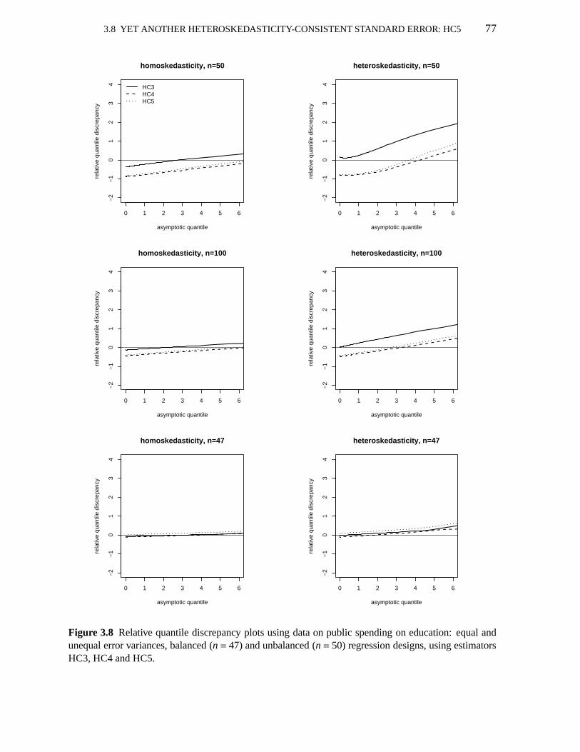
3.8 YET ANOTHER HETEROSKEDASTICITY-CONSISTENT STANDARD ERROR: HC5 77
0 1 2 3 4 5 6
−2
−1
01
23
4
asymptotic quantile
rela
tive
quan
tile
disc
repa
ncy
HC3HC4HC5
homoskedasticity, n=50
0 1 2 3 4 5 6
−2
−1
01
23
4
asymptotic quantile
rela
tive
quan
tile
disc
repa
ncy
heteroskedasticity, n=50
0 1 2 3 4 5 6
−2
−1
01
23
4
asymptotic quantile
rela
tive
quan
tile
disc
repa
ncy
homoskedasticity, n=100
0 1 2 3 4 5 6
−2
−1
01
23
4
asymptotic quantile
rela
tive
quan
tile
disc
repa
ncy
heteroskedasticity, n=100
0 1 2 3 4 5 6
−2
−1
01
23
4
asymptotic quantile
rela
tive
quan
tile
disc
repa
ncy
homoskedasticity, n=47
0 1 2 3 4 5 6
−2
−1
01
23
4
asymptotic quantile
rela
tive
quan
tile
disc
repa
ncy
heteroskedasticity, n=47
Figure 3.8 Relative quantile discrepancy plots using data on public spending on education: equal andunequal error variances, balanced (n= 47) and unbalanced (n= 50) regression designs, using estimatorsHC3, HC4 and HC5.
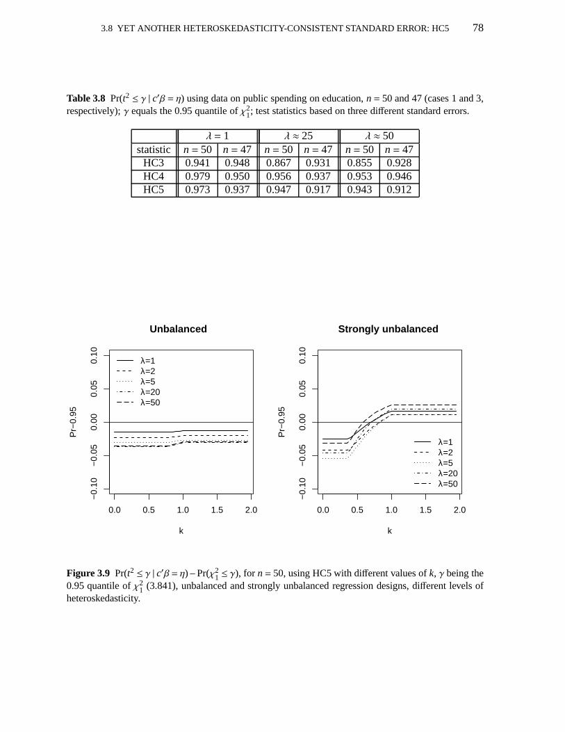
3.8 YET ANOTHER HETEROSKEDASTICITY-CONSISTENT STANDARD ERROR: HC5 78
Table 3.8 Pr(t2 ≤ γ | c′β = η) using data on public spending on education,n= 50 and 47 (cases 1 and 3,respectively);γ equals the 0.95 quantile ofχ2
1; test statistics based on three different standard errors.
λ = 1 λ ≈ 25 λ ≈ 50statistic n= 50 n= 47 n= 50 n= 47 n= 50 n= 47
HC3 0.941 0.948 0.867 0.931 0.855 0.928HC4 0.979 0.950 0.956 0.937 0.953 0.946HC5 0.973 0.937 0.947 0.917 0.943 0.912
0.0 0.5 1.0 1.5 2.0
−0.
10−
0.05
0.00
0.05
0.10
k
Pr−
0.95
λ=1λ=2λ=5λ=20λ=50
Unbalanced
0.0 0.5 1.0 1.5 2.0
−0.
10−
0.05
0.00
0.05
0.10
k
Pr−
0.95
λ=1λ=2λ=5λ=20λ=50
Strongly unbalanced
Figure 3.9 Pr(t2 ≤ γ | c′β = η)−Pr(χ21 ≤ γ), for n= 50, using HC5 with different values ofk, γ being the
0.95 quantile ofχ21 (3.841), unbalanced and strongly unbalanced regression designs, different levels of
heteroskedasticity.
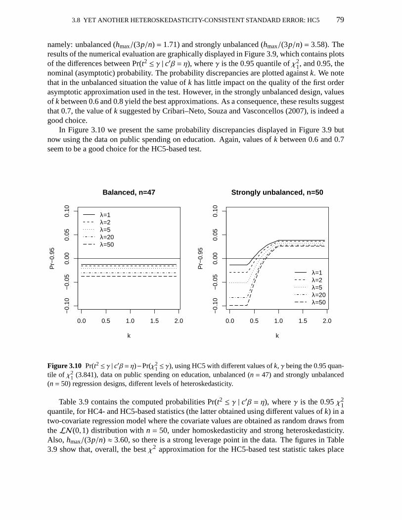
3.8 YET ANOTHER HETEROSKEDASTICITY-CONSISTENT STANDARD ERROR: HC5 79
namely: unbalanced (hmax/(3p/n) = 1.71) and strongly unbalanced (hmax/(3p/n) = 3.58). Theresults of the numerical evaluation are graphically displayed in Figure 3.9, which contains plotsof the differences between Pr(t2 ≤ γ | c′β = η), whereγ is the 0.95 quantile ofχ2
1, and 0.95, thenominal (asymptotic) probability. The probability discrepancies are plotted againstk. We notethat in the unbalanced situation the value ofk has little impact on the quality of the first orderasymptotic approximation used in the test. However, in the strongly unbalanced design, valuesof k between 0.6 and 0.8 yield the best approximations. As a consequence, these results suggestthat 0.7, the value ofk suggested by Cribari–Neto, Souza and Vasconcellos (2007),is indeed agood choice.
In Figure 3.10 we present the same probability discrepancies displayed in Figure 3.9 butnow using the data on public spending on education. Again, values ofk between 0.6 and 0.7seem to be a good choice for the HC5-based test.
0.0 0.5 1.0 1.5 2.0
−0.
10−
0.05
0.00
0.05
0.10
k
Pr−
0.95
λ=1λ=2λ=5λ=20λ=50
Balanced, n=47
0.0 0.5 1.0 1.5 2.0
−0.
10−
0.05
0.00
0.05
0.10
k
Pr−
0.95
λ=1λ=2λ=5λ=20λ=50
Strongly unbalanced, n=50
Figure 3.10 Pr(t2≤ γ | c′β= η)−Pr(χ21 ≤ γ), using HC5 with different values ofk, γ being the 0.95 quan-
tile of χ21 (3.841), data on public spending on education, unbalanced (n = 47) and strongly unbalanced
(n= 50) regression designs, different levels of heteroskedasticity.
Table 3.9 contains the computed probabilities Pr(t2 ≤ γ | c′β = η), whereγ is the 0.95χ21
quantile, for HC4- and HC5-based statistics (the latter obtained using different values ofk) in atwo-covariate regression model where the covariate valuesare obtained as random draws fromtheLN(0,1) distribution withn = 50, under homoskedasticity and strong heteroskedasticity.Also, hmax/(3p/n) ≈ 3.60, so there is a strong leverage point in the data. The figuresin Table3.9 show that, overall, the bestχ2 approximation for the HC5-based test statistic takes place

3.8 YET ANOTHER HETEROSKEDASTICITY-CONSISTENT STANDARD ERROR: HC5 80
whenk= 0.6,0.7. Using these values ofk the HC5 test slightly outperforms the HC4 test.
Table 3.9 Pr(t2 ≤ γ | c′β = η) for n = 50; γ equals the 0.95 quantile ofχ21; test statistics based on HC4
and HC5 (different values ofk) standard errors.
test statistic λ = 1 λ ≈ 50HC5 (k= 0.5) 0.942 0.917HC5 (k= 0.6) 0.956 0.943HC5 (k= 0.7) 0.968 0.960HC5 (k= 0.8) 0.976 0.970HC5 (k= 0.9) 0.981 0.977HC5 (k= 1.0) 0.986 0.983
HC4 0.973 0.967
We shall now report the results of a 10,000 replication MonteCarlo experiment where thenull rejection probabilities of HC4 and HC5 (different values ofk) tests are computed. Themodel used in the evaluation is
yt = β0+β1x1t +β2x2t +εt, t = 1, . . . ,50.
Table 3.10 Null rejection rates of HC4 and HC5 quasi-t tests; HC5 standard errors are computed usingdifferent values ofk; nominal level: 5%.
hmax/(3p/n)3.60 1.14
test statistic λ = 1 λ ≈ 50 λ = 1 λ ≈ 50HC5 (k = 0.5) 5.42 8.47 7.20 8.09HC5 (k = 0.6) 4.04 5.88 7.20 8.09HC5 (k = 0.7) 2.83 4.25 7.20 8.09HC5 (k = 0.8) 2.17 3.23 7.20 8.09HC5 (k = 0.9) 1.64 2.44 7.20 8.09HC5 (k = 1.0) 1.28 1.82 7.20 8.09
HC4 2.40 3.56 5.72 6.37
The errors are uncorrelated, eachεt being normally distributed with zero mean and varianceσ2
t = exp(α1x1t +α2x2t). The covariate values were selected as random draws from the stan-dard lognormal distribution. Simulations were performed under both homoskedasticity (λ = 1)and heteroskedasticity (λ ≈ 50) and we consider two different settings in which the values ofhmax/(3p/n) are 3.60 and 1.14. The interest lies in testingH0 : β2 = 0 againstH1 : β2 , 0. Datageneration was carried out usingβ0 = β1 = 1 andβ2 = 0. The quasi-t test statistics consideredemploy HC4 and HC5 (k= 0.5,0.6,0.7,0.8,0.9,1.0) standard errors.
3.9 CONCLUDING REMARKS 81
Table 3.10 presents the null empirical rejection rates at the nominal levelα = 0.05. Allentries are percentages. When leverage is strong (hmax/(3p/n) ≈ 3.60), k = 0.6 overall yieldsthe best HC5 test. When leverage is weak, however, the HC5 test is outperformed by HC4regardless the value ofk.
3.9 Concluding remarks
We have considered the issue of making inference on the parameters that index the linear re-gression model under heteroskedasticity of unknown form. We have numerically evaluatedthe first order asymptotic approximation used in quasi-t tests. Our evaluation didnot rely onMonte Carlo simulations.7 Rather, we assumed normality, wrote the test statistics as ratios ofquadratic forms in a vector of uncorrelated standard normalvariates, and used Imhof’s (1961)numerical integration algorithm to compute the exact distribution functions of the differenttest statistics. We have included in the analysis test statistics that use standard errors obtainedfrom the widely used HCCME proposed by Halbert White (HC0) and from HC3, an oftenpraised HCCME (e.g., Long and Ervin, 2000). In addition, we included alternative test statis-tics based on several recently proposed heteroskedasticity-robust standard errors, namely: HC4(Cribari–Neto, 2004),V1 andV2 (Qian and Wang, 2001), and HC5 (Cribari–Neto, Souza andVasconcellos, 2007). We have also made use of numerical integration methods to shed lighton the choice of constants used in the definitions ofV2 and HC5. Our main findings can beoutlined as follows:
i Under equal error variances and in balanced regression designs, the null distributions of alltest statistics are typically well approximated by the limiting null distribution, from whichwe obtain critical values for the tests;
ii Under homoskedasticity and leveraged data, the best first order asymptotic approximationsare those for the HC4- and HC5-based tests;
iii Under heteroskedasticity and in balanced regression designs, the tests based on HC3, HC4,HC5, V1 andV2(a) with a= 0 anda= 2 appear to be reliable in finite samples;
iv The best performing tests under heteroskedasticity and leveraged data are those whose teststatistics use standard errors from HC4, HC5 andV2(15).
Since in practice we have no knowledge of the strength of heteroskedasticity and leveragepoints are often present in the data, we recommend the use of HC4-based tests or HC5-basedtests withk= 0.6 ork= 0.7 when leverage is very intense.
7We only used Monte Carlo simulation once in our analysis: to estimate the null rejection rates of differentHC5 tests. All other numerical evaluations were carried outin exact fashion by using a numerical integrationmethod.

C 4
Conclusions
The object of interest of this doctoral dissertation was thelinear regression model. The assump-tion that all error variances are equal (homoskedasticity)is commonly violated in regressionanalysis that use cross-sectional data. It is thus important to develop and evaluate inferencestrategies that are robust to heteroskedasticity. This wasour main motivation.
At the outset, we have proposed different heteroskedasticity-consistent interval estimators(HCIEs) for the regression parameters. They are based on variance and covariance estimatorsthat are asymptotically correct under heteroskedasticityof unknown form and also under equalerror variances. We have also considered bootstrap-based interval estimators. Our numericalevaluation revealed that the HC4 HCIE outperforms all otherinterval estimators, includingthose that employ bootstrap resampling.
We then moved to point estimation of variances and covariances. We considered a heteros-kedasticity-consistent covariance matrix estimator (HCCME) proposed by L. Qian and S. Wangin 2001, which is a modified version of the well known White estimator. We have obtained asequence of bias-adjusted estimators in which the biases vanish at faster rates as we move alongthe sequence. We have also generalized the Qian–Wang estimator, and obtained alternativesequences of improved estimators. Our numerical results have shown that the proposed bias-adjusting schemes can be quite effective in small samples.
Finally, we addressed the issue of performing hypothesis testing inference in the linear re-gression model under heteroskedasticity of unknown form. We have added the Gaussianityassumption and used a numerical integration algorithm to compute the exact distribution func-tions of different quasi-t test statistics, which were then compared to the respectivelimitingnull distribution. To that end, we have shown that such statistics can be written as ratios ofquadratic forms in standard normal (Gaussian) random vectors. We focused on test statisticsthat use four recently proposed heteroskedasticity-robust standard errors. Two of them employconstants that are chosen in anad hocmanner, and our results have shed light on their optimalvalues. Overall, our numerical evaluations favored the HC4-based test.
82
C 5
Resumo do Capítulo 1
5.1 Introdução
O modelo de regressão linear é comumente utilizado para modelar a relação entre uma variávelde interesse e um conjunto de variáveis explicativas. Quando dados de corte transversal sãousados, a suposição de que os erros do modelo têm a mesma variância (homoscedasticidade)é freqüentemente violada. Uma prática comum é usar o estimador de mínimos quadrados or-dinários (EMQO) em conjunção com um estimador consistente de sua matriz de covariânciasquando o interesse reside em inferências por testes de hipóteses. Nesse capítulo, o nosso focorecai sobre inferências através de estimadores intervalares. Nós propomos e avaliamos nu-mericamente diferentes estimadores intervalares robustos à presença de heteroscedasticidade,inclusive estimadores baseados em esquemas de reamostragem de bootstrap.
5.2 O modelo e alguns estimadores pontuais
O modelo de interesse é o modelo de regressão linear
y= Xβ+ε,
ondey é um vetor de observações de dimensãon na variável dependente,X é uma matrizfixa n× p de regressores (posto(X) = p < n), β = (β0, . . . ,βp−1)′ é um p-vetor de parâmetrosdesconhecidos eε = (ε1, . . . , εn)′ é um vetorn-dimensional de erros aleatórios. As suposições aseguir são comumente feitas:
A1 O modeloy= Xβ+ε está corretamente especificado;
A2 E(εi) = 0, i = 1, . . . ,n;
A3 E(ε2i ) = var(εi) = σ2i (0< σ2
i <∞), i = 1, . . . ,n;
A3’ var(εi) = σ2, i = 1, . . . ,n (0< σ2 <∞);
A4 E(εiε j) = 0 ∀ i , j;
A5 limn→∞n−1(X′X) = Q, ondeQ é uma matrix positiva definida.
83
5.2 O MODELO E ALGUNS ESTIMADORES PONTUAIS 84
Sob [A1], [A2], [A3] and [A4], a matriz de covariâncias deε é
Ω = diagσ2i ,
que se reduz aΩ = σ2In quandoσ2i = σ
2 > 0, i = 1, . . . ,n, i.e.,sob [A3’] (homoscedasticidade),ondeIn é a matriz identidade de ordemn.
O EMQO ofβ é obtido minimizando a soma de quadrados dos erros, i.e., minimizando
ε′ε = (y−Xβ)′(y−Xβ);
o estimador pode ser escrito em forma fechada como
β = (X′X)−1X′y.
Suponha que [A1] é verdadeira. Pode ser mostrado que:i) Sob [A2], β é não viesado paraβ, i.e.,E(β) = β ∀β ∈ IRp.
ii) Ψβ= var(β) = (X′X)−1X′ΩX(X′X)−1.
iii) Sob [A2], [A3], [A5] e também considerando as variâncias uniformemente limitadas,βé um estimador consistente paraβ, i.e., plim
(β)= β, onde plim denota limite em probabilidade.
iv) Sob [A2], [A3’] e [A4], β é o melhor estimador linear não-viesado deβ (Teorema deGauss–Markov) .
De ii), notamos que sob homoscedasticidade var(β) = σ2(X′X)−1, que pode ser facilmenteestimado comovar(β) = σ2(X′X)−1, ondeσ2 = ε′ε/(n− p) e ε é o vetor de resíduos do ajustepor mínimos quadrados:
ε = y−Xβ = In−X(X′X)−1X′y= (In−H)y.
A matriz H = X(X′X)−1X′ é chamada de ‘matriz chapéu’, uma vez queHy = y. Seus ele-mentos diagonais assumem valores no intervalo (0,1) e somamp, o posto deX, sendo portantosua médiap/n. Observe-se que os elementos diagonais deH (h1, . . . ,hn) são comumente u-sados como medidas de alavancagem das correspondentes observações; observações tais quehi > 2p/n ou hi > 3p/n são consideradas pontos de alavanca (veja Davidson and MacKinnon,1993).
Sob heteroscedasticidade, quando conhecemos a matrizΩ ou uma função cedástica quenos permita estimarΩ, podemos estimarβ utilizando o estimador de mínimos quadradosgeneralizado (EMQG) ou o estimador de mínimos quadrados generalizado viável (EMQGV).Para realizar inferências sobreβ que sejam válidas assintoticamente sob heteroscedasticidade,costuma-se utilizar o EMQO deβ, que permanece consistente, não-viesado e assintoticamentenormal, conjuntamente com um estimador consistente de sua matriz de covariâncias.
White (1980) derivou um estimador consistente paraΨβ
observando que não é necessárioestimar consistentementeΩ (que temn parâmetros desconhecidos); é necessário apenas esti-mar consistentementeX′ΩX (que temp(p+ 1)/2 elementos distintos independentemente dotamanho da amostra).1 Necessita-se apenas encontrarΩ tal que plim
((X′ΩX)−1(X′ΩX)
)= Ip.
1Para estimar consistentemente a matriz de covariâncias, sob heteroscedasticidade, também supomos:
A6 limn→∞n−1(X′ΩX) = S, ondeS é uma matriz positiva definida.
5.3 ESTIMADORES INTERVALARES CONSISTENTES SOB HETEROSCEDASTICIDADE 85
O estimador de White, também conhecido como HC0, é obtido substituindo oi-ésimo elementodiagonal deΩ na expressão paraΨ
βpelo quadrado doi-ésimo resíduo de mínimos quadrados,
i.e.,HC0= (X′X)−1X′Ω0X(X′X)−1,
ondeΩ0 = diagε2i .O estimador de White é consistente sob homoscedasticidade esob heteroscedasticidade
de forma desconhecida. Entretanto, ele pode ser bastante viesado em amostras finitas, comoevidenciado pelos resultados numéricos obtidos por Cribari–Neto e Zarkos (1999, 2001). Adi-cionalmente, a magnitude do viés é inflacionada quando o desenho de regressão contém pontosde alavanca.
Algumas variantes do HC0 foram propostas na literatura. Essas variantes incluem correçõespara amostras finitas na estimação deΩ e são dadas por:
i (Hinkley, 1977) HC1= Ψ1 = PΩ1P′ = PD1ΩP′, ondeD1 = (n/(n− p))I ;
ii (Horn, Horn e Duncan, 1975) HC2= Ψ2 = PΩ2P′ = PD2ΩP′, onde
D2 = diag1/(1−hi);
iii (Davidson e MacKinnon, 1993) HC3= Ψ3 = PΩ3P′ = PD3ΩP′, onde
D3 = diag1/(1−hi)2;
iv (Cribari–Neto, 2004) HC4= Ψ4 = PΩ4P′ = PD4ΩP′, onde
D4 = diag1/(1−hi)δi , δi =min4,nhi/p.
5.3 Estimadores intervalares consistentes sob heteroscedasticidade
Nosso principal interesse consiste em obter intervalos de confiança para os parâmetros desco-nhecidos do modelo de regressão.
Consideramos ‘heteroskedasticity-consistent interval estimators’ (HCIEs) baseados emβ(EMQO) e nos ‘heteroskedasticity-consistent covariance matrix estimators’ (HCCMEs) HC0,HC2, HC3 e HC4. Sob homoscedasticidade e quando os erros são normalmente distribuídos, aquantidade
β j −β j√σ2c j j
,
ondec j j é o j-ésimo elemento diagonal de (X′X)−1, tem distribuiçãotn−p, sendo então fácilconstruir intervalos de confiança exatos paraβ j , j = 0, . . . , p−1.
Sob heteroscedasticidade, a matriz de covariâncias do EMQOé
Ψβ= var(β) = (X′X)−1X′ΩX(X′X)−1.
5.4 AVALIAÇÃO NUMÉRICA 86
Os estimadores consistentes apresentados anteriormente são estimadores do tipo sanduíche paraa matriz de covariâncias. A seguir usaremos os estimadores HCk, k = 0,2,3,4. Seja, parak= 0,2,3,4,
Ωk = DkΩ = Dkdiagε2i ;para HC0,D0 = In;para HC2,D2 = diag1/(1−hi);para HC3,D3 = diag1/(1−hi)2;para HC4,D4 = diag1/(1−hi)δi .Portanto,
Ψ(k)
β= (X′X)−1X′ΩkX(X′X)−1, k= 0,2,3,4.
Parak= 0,2,3,4, considere a quantidade
β j −β j√Ψ
(k)j j
,
ondeΨ(k)j j é o j-ésimo elemento diagonal deΨ(k)
β, i.e., a variância estimada deβ j obtida do
estimador HCk, k = 0,2,3,4. Segue-se da normalidade assintótica ofβ j e da consistência deΨ
(k)j j que a quantidade acima converge em distribuição à distribuição normal padrão quando
n→∞. Portanto, essa quantidade pode ser usada para construir HCIEs. Seja 0< α < 1/2. Umaclasse de intervalos de confiança com cobertura de (1−α)×100% paraβ j , j = 0, . . . , p−1, é
β j ±z1−α/2
√Ψ
(k)j j ,
k= 0,2,3,4, ondez1−α/2 é o quantil 1−α/2 da distribuição normal padrão.
5.4 Avaliação numérica
A avaliação de Monte Carlo usa o seguinte modelo de regressãolinear:
yi = β0+β1xi +σiεi , i = 1, . . . ,n,
ondeεi ∼ (0,1) eE(εiε j) = 0∀i , j. Aqui,
σ2i = σ
2expaxi
comσ2 = 1. São considerados erros normais bem como erros exponenciais (com média um)e erros obtidos de uma distribuição de caudas pesadas (t3). Estimaremos numericamente asprobabilidades de cobertura dos diferentes HCIEs e calcularemos seus comprimentos médios.Os valores da covariável foram selecionados aleatoriamente da distribuiçãoU(0,1) bem comoda distribuiçãot3; no segundo caso, o desenho de regressão contém pontos de alavanca. Ostamanhos de amostra sãon = 20,60,100. Nós geramos 20 valores da covariável quando o
5.5 INTERVALOS BOOTSTRAP 87
tamanho da amostra én = 20; para tamanhos maiores esses valores foram replicados três ecinco vezes (n= 60 en= 100, respectivamente) de modo que o nível de heteroscedasticidade,medido por
λ =maxσ2i /minσ2
i , i = 1, . . . ,n,
permanece constante quando o tamanho da amostra aumenta. Consideramos o caso homoscedás-tico (λ = 1) e dois níveis de heteroscedasticidade (λ ≈ 9 eλ ≈ 49). Para gerar os valores deyutilizamosβ0 = β1 = 1. O número de réplicas de Monte Carlo foi 10,000 e todas as simulaçõesforam realizadas utilizando a linguagem de programaçãoOx (Doornik, 2001).
A cobertura nominal de todos os intervalos é 1−α = 0.95. O intervalo de confiança padrão(MQO) usou erros padrão deσ2(X′X)−1 e foi calculado como
β j ± t1−α/2,n−2
√σ2c j j ,
ondet1−α/2,n−2 é o quantil 1−α/2 da distribuiçãotn−2. Os HCIEs foram calculados como
β j ± z1−α/2
√Ψ
(k)j j ,
k= 0,2,3,4 (HC0, HC2, HC3 e HC4, respectivamente).Os resultados encontram-se apresentados nas Tabelas 1.2, 1.3, 1.4 e 1.5 do Capítulo 1.
Observa-se que os intervalos obtidos com o estimador HC0 podem ser bastante ruins quandoo tamanho da amostra não é grande. Os resultados favorecem o estimador intervalar HC4, queapresenta comportamento mais confiável do que aqueles apresentados pelos intervalos obtidoscom HC0 e HC2 e mesmo com HC3.
5.5 Intervalos bootstrap
Um enfoque alternativo é usar reamostragem dos dados para obter intervalos de confiança;em particular utilizaremos o método bootstrap proposto porBradley Efron (Efron, 1979). Obootstrap ponderado de Wu (1986) pode ser usado para se obtererros-padrão assintoticamentecorretos sob heteroscedasticidade de forma desconhecida.Nós propomos utilizar o intervalode confiança bootstrap percentil combinado com um esquema dereamostragem baseado embootstrap ponderado. A construção dos intervalos paraβ j ( j = 0, . . . , p−1) pode ser feita comose segue.
S1 Para cadai, i = 1, . . . ,n, obtenhat∗i aleatoriamente de uma população com média zero evariância unitária;
S2 Construa uma amostra bootstrap (y∗,X), onde
y∗i = xi β+ t∗i εi/√
1−hi ,
sendoxi a i-ésima linha deX;
S3 Calcule o EMQO deβ: β∗ = (X′X)−1X′y∗;
5.6 REGIÕES DE CONFIANÇA 88
S4 Repita os passos 1 a 3 um grande número de vezes (por exemplo,B vezes);
S5 Os limites inferior e superior do intervalo com (1−α)×100% de confiança paraβ j (0< α <1/2) são, respectivamente, os quantisα/2 e 1−α/2 dasB réplicas bootstrapβ∗j .
A quantidadet∗i , i = 1, . . . ,n, deve ser amostrada aleatoriamente de uma população commédia zero e variância unitária.
Comparamos, usando simulação Monte Carlo, o comportamentoem amostras finitas dosHCIEs descritos anteriormente com o estimador intervalar híbrido (percentil/ponderado) des-crito acima (Tabela 1.6). Inferências são realizadas sobreo parâmetroβ1, o número de réplicasMonte Carlo foi 5,000 e o número de replicações bootstrap foiB = 500. Da comparação daTabela 1.6 com as Tabelas 1.2, 1.3, 1.4 e 1.5 do Capítulo 1, concluímos que os intervalos HC4apresentam melhor desempenho que os intervalos bootstrap.
Foram utilizados mais três estimadores bootstrap alternativos, que também são baseados nométodo percentil mas usam diferentes esquemas de reamostragem. O primeiro estimador alter-nativo emprega o bootstrap selvagem de Liu (1988); o segundoestimador, chamado de (y,X)bootstrap, utiliza, em vez de resíduos, reamostragem de pares (xi ,yi), i = 1, . . . ,n; e o último esti-mador intervalar bootstrap utilizado combina reamostragem ponderada com o método percentilt (ver Efron e Tibshirani, 1993, pp.160–162). As taxas estimadas de cobertura e as amplitudesmédias destes intervalos bootstrap estão nas Tabelas 1.7 e 1.8. Entre os intervalos bootstrap,o melhor desempenho quandon = 20 é do intervalo (y,X) bootstrap e o melhor desempenhoquando o tamanho da amostra é grande (n= 100) cabe ao intervalo bootstrap percentilt. Note,todavia, que os intervalos HC4 têm melhor desempenho do que todos os intervalos bootstrap.
5.6 Regiões de confiança
Nesta seção consideramos a obtenção de regiões de confiança assintoticamente válidas sobheteroscedasticidade de forma desconhecida. Escrevemos omodelo de regressão
y= Xβ+ε
comoy= X1β1+X2β2+ε, (5.6.1)
ondey, X, β e ε são como descritos na Seção 5.2,X j e β j sãon× p j e p j ×1, respectivamente,j = 1,2, comp= p1+ p2 tal queX = [X1 X2] e β = (β′1,β
′2)′.
O EMQO do vetor dos coeficientes de regressão em 5.6.1 éβ =(β′1, β
′2
)′, onde
β2 =(R′2R2
)−1R′2y,
comR2 =M1X2 e M1 = In−X1(X′1X1)−1X′1. Dado queβ2 é assintoticamente normal com médiaβ2 e matriz de covariâncias
V22=(R′2R2
)−1R′2ΩR2
(R′2R2
)−1,
5.6 REGIÕES DE CONFIANÇA 89
a forma quadráticaW=
(β2−β2
)′V−1
22
(β2−β2
)
é assintoticamenteχ2p2
. Este resultado permanece verdadeiro quandoV22 é substituído por umafunção dos dadosV22 tal que plim
(V22
)= V22. Em particular, nós podemos usar o seguinte
estimador consistente da matriz de covariância deβ2:
V(k)22 = (R′2R2)−1R′2ΩkR2(R′2R2)−1,
ondeΩk, k= 0,2,3,4, é como definido na Seção 5.2.Seja 0< α < 1 e sejaχ2
p2,αtal que
Pr(χ2p2< χ2
p2,α) = 1−α;
isto é,χ2p2,α
é o quantil 1−α da distribuiçãoχ2p2
. Considere também
W(k) =(β2−β2
)′ (V(k)
22
)−1 (β2−β2
).
Então, a região com 100× (1−α)% de confiança paraβ2 é dada pelo conjunto de valores deβ2
tal queW(k) < χ2
p2,α. (5.6.2)
Avaliaremos numericamente os desempenhos em amostras finitas das diferentes regiões deconfiança. O modelo de regressão usado na simulação é
yi = β0+β1xi1+β2xi2+εi , i = 1, . . . ,n,
ondeεi é um erro distribuído normalmente com média zero.Os valores das covariáveis foram obtidos como realizações da distribuição uniforme padrão
(desenho balanceado) e da distribuiçãot3 (desenho não-balanceado). O número de réplicas deMonte Carlo foi 10,000, os tamanhos amostrais consideradosforamn = 20,60,100 e 1−α =0.95. As simulações foram realizadas sob homoscedasticidadee sob heteroscedasticidade. Ascoberturas apresentadas correspondem às percentagens dasréplicas nas quais (5.6.2) se verificaquando são realizadas inferências conjuntas sobreβ1 eβ2. A fim de comparar os desempenhosdas regiões de confiança (‘joint’) e dos intervalos de confiança (paraβ1 eβ2 separadamente) ascoberturas individuais são também apresentadas na Tabela 1.10.
Observamos inicialmente na Tabela 1.10 que as coberturas conjuntas são sempre menoresque as individuais. No geral, observamos que a região de confiança HC4 é a que tem melhordesempenho, especialmente quando os dados são não-balanceados. A região de confiança HC3é competitiva quando o desenho de regressão é balanceado.
C 6
Resumo do Capítulo 2
6.1 Introdução
A suposição de homoscedasticidade, quando são usados dadostransversais nos modelos de re-gressão, é freqüentemente violada. Erros-padrão consistentes para o estimador de mínimosquadrados ordinários (EMQO) podem ser obtidos seguindo o enfoque proposto por White(1980). No entanto, estes erros-padrão são bastante viesados em amostras pequenas. Qiane Wang (2001), propuseram um estimador menos viesado que o proposto por White. Nestecapítulo, nós definimos uma seqüência de estimadores ajustados pelo viés a partir do estimadorproposto por Qian e Wang, melhorando sua precisão. Mostramos ainda, que o estimador deQian e Wang pode ser generalizado para uma classe mais ampla de estimadores consistentessob heteroscedasticidade e que os resultados obtidos para oestimador de Qian e Wang podemser facilmente estendidos a esta classe de estimadores.
6.2 O modelo e estimadores da matriz de covariâncias
Considere toda a seção dois do Capítulo 4 para definição do modelo e dos estimadores HC0,HC1, HC2, HC3 e HC4.
Como observamos no Capítulo 4, o estimador HC0 é consideravelmente viesado em amos-tras de tamanho pequeno a moderado. Cribari–Neto, Ferrari and Cordeiro (2000) obtiveramvariantes do estimador HC0 usando um mecanismo iterativo decorreção de viés. A cadeia deestimadores foi obtida corrigindo HC0, em seguida corrigindo o estimador resultante e assimpor diante.
Seja (A)d a matriz diagonal obtida fazendo os elementos não-diagonais da matriz quadradaA iguais a zero. Note queΩ = (εε′)d. Então,
E(εε′) = cov(ε)+E(ε)E(ε′)
= (I −H)Ω(I −H)
dado que (I −H)X = 0. Segue-se queE(Ω) = (I −H)Ω(I −H)d eE(Ψ) = PE(Ω)P′. Portanto,os vieses deΩ e Ψ como estimadores deΩ eΨ são
BΩ
(Ω) = E(Ω)−Ω = HΩ(H −2I )d
eBΨ
(Ω) = E(Ψ)−Ψ = PBΩ
(Ω)P′,
90

6.2 O MODELO E ESTIMADORES DA MATRIZ DE COVARIÂNCIAS 91
respectivamente.Cribari–Neto, Ferrari and Cordeiro (2000) definem o estimador corrigido pelo viés
Ω(1) = Ω−BΩ
(Ω).
Este estimador pode ser por sua vez corrigido pelo viés:
Ω(2) = Ω(1)−BΩ(1)(Ω),
e assim sucessivamente. Apósk iterações do esquema de correção obtém-se
Ω(k) = Ω(k−1)−BΩ(k−1)(Ω).
Considere a seguinte função recursiva de uma matriz diagonal A n×n:
M(k+1)(A) = M(1)(M(k)(A)), k= 0,1, . . . ,
ondeM(0)(A)= A, M(1)(A)= HA(H−2I )d, eH é como definido anteriomente. Podemos entãoescreverB
Ω(Ω) = M(1)(Ω). Por indução, pode ser mostrado que o estimador dek-ésima ordem
corrigido pelo viés e seu respectivo viés podem ser escritoscomo
Ω(k) =
k∑
j=0
(−1) j M( j)(Ω)
e
BΩ(k)(Ω) = (−1)kM(k+1)(Ω),
parak= 1,2, . . ..Define-se então uma seqüência de estimadores corrigidos pelo viés para a matriz de cova-
riâncias comoΨ(k),k= 1,2, . . ., onde
Ψ(k) = PΩ(k)P′. (6.2.1)
O viés deΨ(k) é
BΨ(k)(Ω) = (−1)kPM(k+1)(Ω)P′,
k= 1,2, . . ..Mostra-se queB
Ψ(k)(Ω) = O(n−(k+2)), isto é, o viés do estimador corrigidok vezes é deordemO(n−(k+2)), enquanto que o viés do estimador de White éO(n−2).
6.3 UMA NOVA CLASSE DE ESTIMADORES AJUSTADOS PELO VIÉS 92
6.3 Uma nova classe de estimadores ajustados pelo viés
Um estimador alternativo foi proposto por Qian e Wang (2001). Veremos que este estimadoré uma variante do estimador HC0 corrigido pelo viés. SejaK = (H)d = diagh1, . . . ,hn, i.e.,Ké a matriz diagonal que contém as medidas de alavancagem, e seja Ci = X(X′X)−1x′i a i-ésimacoluna da matrizH, ondexi é ai-ésima linha deX, i = 1, . . . ,n.
Seguindo Qian and Wang (2001), definimos
D(1) = diagdi = diag(ε2i − bi)gii ,
ondegii = (1+C′i KCi −2h2
i )−1
ebi =C′i (Ω− 2ε2i I )Ci .
O estimador de Qian–Wang é definido como
V(1) = PD(1)P′. (6.3.1)
Mostraremos inicialmente que o estimador em (6.3.1) é uma versão corrigida pelo viés doestimador proposto por White a menos de um fator de correção.Note que
di = (ε2i − bi)gii
= (ε2i −C′i ΩCi + 2ε2i C′i Ci)gii . (6.3.2)
Fazendok = 1 (correção de primeira ordem), o estimador corrigido pelo viés em (6.2.1) podeser escrito comoΨ(1) = PΩ(1)P′, onde
Ω(1) = Ω−M(1)(Ω)
= Ω−HΩ(H −2I )d= diagε2i −C′i ΩCi + 2ε2i hi. (6.3.3)
Dado quehi =C′i Ci , é fácil ver que (6.3.2) é igual aoi-ésimo elemento da diagonal deΩ(1) em(6.3.3), a menos da multiplicação porgii . Então,
D(1) = [Ω−HΩ(H −2I )d]G,
ondeG= I +HKH −2KK−1d .
Qian and Wang (2001) mostraram queV(1) é não-viesado paraΨ sob homoscedasticidade.Utilizando o esquema de correção pelo viés descrito anteriormente, mostra-se que a forma
geral do estimador de Qian-Wang corrigidok vezes é
V(k) = PD(k)P′, (6.3.4)
com
6.4 ESTIMAÇÃO DA VARIÂNCIA DE COMBINAÇÕES LINEARES DOS ELEMENTOS DEβ 93
D(k) = 1(k>1)×M(0)(Ω)+1(k>2)×k−2∑
j=1
(−1) j M( j)(Ω)
+
k∑
j=k−1
(−1) j M( j)(Ω)G, (6.3.5)
k= 1,2, . . ., onde 1(·) é a função indicadora. Seu viés é
BD(k)(Ω) = (−1)k−1M(k−1)(Ω)(G− I )
+ (−1)kM(k+1)(Ω)G, (6.3.6)
k= 1,2, . . ..Definimos então a seqüênciaV(k),k= 1,2, . . . de estimadores paraΨ. O viés deV(k) segue
de (6.3.6) e (6.3.4):
BV(k)(Ω) = P[BD(k)(Ω)]P′. (6.3.7)
Mostra-se que a ordem dos vieses em (6.3.7) é
BD(k)(Ω) =O(n−(k+1)),
o que leva aBV(k)(Ω) =O(n−(k+2)).
Portanto, a ordem do viés do estimador de Qian-Wang de ordemk é a mesma do estimadorde White de mesma ordem como em Cribari–Neto, Ferrari e Cordeiro (2000); ver Seção 6.2.(Lembre, entretanto, quek = 1 aqui, indica o estimador de Qian-Wang não-modificado, o qualé uma correção de primeira ordem do estimador de White).
6.4 Estimação da variância de combinações lineares dos elementos deβ
Sejac um p-vetor de constantes tal quec′β é uma combinação linear dos elementos deβ.Definimos
Φ = var(c′β) = c′[cov(β)]c= c′Ψc.
O estimador corrigido dek-ésima ordem, dado em (6.3.4), é
V(k) = Ψ(k)QW = PD(k)P′
e, dessa forma,Φ
(k)QW = c′Ψ(k)
QWc= c′PD(k)P′c
é o elemento de ordemk de uma seqüência de estimadores ajustados pelo viés paraΦ, ondeD(k), k= 1,2, . . ., é definido na equação (6.3.5).
6.4 ESTIMAÇÃO DA VARIÂNCIA DE COMBINAÇÕES LINEARES DOS ELEMENTOS DEβ 94
Lembramos que quandok = 1 nós obtemos o estimador de Qian–Wang. Usando este esti-mador, nós obtemos
Φ(1)QW= c′Ψ(1)
QWc= c′PD(1)P′c,
ondeD(1) = ΩG−M(1)(Ω)G=G1/2ΩG1/2−G1/2M(1)(Ω)G1/2.
SejaW= (ww′)d, ondew=G1/2P′c. Podemos escrever
Φ(1)QW = c′P[G1/2ΩG1/2−G1/2M(1)(Ω)G1/2]P′c
= w′Ωw−w′M(1)(Ω)w.
Note quew′Ωw= w′[( εε′)d]w= ε′[(ww′)d]ε = ε′Wε e que
w′M(1)(Ω)w=n∑
s=1
αsw2s,
ondeαs é o elemento de ordems da diagonal deM(1)(Ω) = HΩ(H −2I )d e ws é o elementode ordems do vetorw. Então,
Φ(1)QW = ε′Wε−
n∑
s=1
αsw2s. (6.4.1)
Mostra-se que a equação (6.4.1) pode ser escrita em forma matricial como
Φ(1)QW = ε′Wε− ε′[M(1)(W)]ε
= ε′[W−M(1)(W)]ε.
Mais geralmente, podemos escrever
Φ(k)QW = ε′Q(k)ε, k= 1,2, . . . , (6.4.2)
ondeQ(k) = 1(k>1)×∑k−2
j=0(−1) j M( j)(B)+∑k
j=k−1(−1) j M( j)(W).
Cribari–Neto, Ferrari e Cordeiro (2000) mostraram que o estimador da variância dec′βusando HC0 é dado por
Φ(k)W = c′Ψ(k)c
= ε′Q(k)W ε, k= 0,1,2, . . . ,
ondeQ(k)W =
∑kj=0(−1) j M( j)(B).
Escrevendo a forma quadrática em (6.4.2) como uma forma quadrática num vetor de vari-áveis aleatórias não-correlacionadas de média zero e variância unitária, temos
Φ(k)QW = a′C(k)
QWa,

6.5 RESULTADOS NUMÉRICOS 95
ondeC(k)QW = Ω
1/2(I −H)Q(k)(I −H)Ω1/2 é uma matriz simétrican×n e a é tal queE(a) = 0 e
cov(a) = I . No que se segue escreveremosC(k)QW simplesmente comoCQW para simplificar a
notação. Mostra-se que, quando os erros são independentes,
var(Φ(k)QW) = d′Λd+2tr(C2
QW), (6.4.3)
onded é um vetor coluna formado pelos elementos diagonais deCQW, tr(CQW) é o traço deCQW eΛ = diagγi, ondeγi = (µ4i −3σ4
i )/σ4i é o excesso de curtose doi-ésimo erro. Quando
os erros são normalmente distribuídos,γi = 0. Então,Λ = 0 e (6.4.3) se torna
var(Φ(k)QW) = var(c′Ψ(k)
QWc) = 2tr(C2QW).
Para a seqüência de estimadores HC0 corrigidos, obtemos (Cribari–Neto, Ferrari e Cordeiro,2000)
var(Φ(k)W ) = 2tr(C2
W),
ondeCW = Ω1/2(I −H)Q(k)
W (I −H)Ω1/2.
6.5 Resultados numéricos
Utilizaremos as expressões exatas dos vieses e das variâncias das combinações lineares deβpara avaliar numericamente a eficiência das correções para amostras finitas dos estimadoresde White (HC0) e Qian–Wang (V(1)). Calcularemos também as raízes quadradas dos errosquadráticos médios e os vieses maximais dos diferentes estimadores.
O modelo usado na avaliação numérica é
yi = β0+β1xi1+β2xi2+εi , i = 1, . . . ,n,
ondeε1, . . . , εn são erros não-correlacionados comE(εi) = 0 e var(εi) = exp(γxi2), i = 1, . . . ,n.Nós usamos diferentes valores deγ a fim de variar o grau de heteroscedasticidade, medidoatravés deλ = maxσ2
i /minσ2i , i = 1, . . . ,n. Os tamanhos de amostra considerados foram
n= 20,40,60. Paran= 20, os valores das covariáveisxi2 e xi3 foram obtidos como realizaçõesaleatórias das distribuições uniforme padrãoU(0,1) e lognormal padrão LN(0,1); sob o últimodesenho os dados contêm pontos de alavanca. Os vinte valoresdas covariáveis foram replicadosduas e três vezes para os tamanhos de amostra 40 e 60, respectivamente. Isto foi feito para queo grau de heteroscedasticidade (λ) não mudasse comn.
As Tabelas 2.2 e 2.3 apresentam o viés relativo total do estimador da variância quando usa-mos os estimadores MQO, HC0 e suas quatro correções e o estimador de Qian-Wang (V(1)) esuas correções até quarta ordem. O viés relativo total é definido como a soma dos valores ab-solutos dos vieses relativos individuais; o viés relativo éa diferença entre a variância estimadade β j e a correspondente variância verdadeira dividida pela variância verdadeira,j = 0,1,2.Observa-se que a correção proposta para o estimador de Qian-Wang é bem efetiva quandon = 20, desenho não-balanceado e sob heteroscedasticidade, apresentando redução de até 23vezes no viés relativo total quandoλ ≈ 49.
6.5 RESULTADOS NUMÉRICOS 96
A Tabela 2.4 contém a raiz quadrada do erro quadrático médio total, que é definido como asoma dos erros quadráticos médios individuais standartizados pelas correspondentes variânciasverdadeiras. Nota-se que os valores correspondentes aos estimadores de Qian-Wang corrigi-dos são aproximadamente iguais aos equivalentes corrigidos do estimador HC0, especialmentequandon= 40,60.
Determinamos também a combinação linear dos estimadores dos parâmetros de regressãocuja variância estimada apresenta viés máximo. Estes vieses maximais são dados pelos auto-valores maximais das matrizes (dos valores absolutos) dos vieses.1 Os resultados estão apre-sentados na Tabela 2.5. Nota-se que a correção iterativa quepropusemos para melhorar o de-sempenho do estimador de Qian-Qang em amostras pequenas pode ser bem efetiva em algunscasos. Por exemplo, quandon = 20,λ ≈ 49 e os valores das covariáveis foram selecionadosda distribuição uniforme, o viés maximal do estimador de Qian-Wang foi reduzido de 0.285 a0.012 (aproximadamente 24 vezes) após quatro iterações do esquema de ajuste pelo viés.
Foi realizado um experimento Monte Carlo com 10000 réplicas, a fim de avaliar o desem-penho, em amostras finitas, de testes quasi-t baseados nos estimadores HC0 e de Qian-Wange suas versões corrigidas até quarta ordem. Utilizou-se um modelo de regressão com duasvariáveis regressorasyi = β1+ β2xi2+ β3xi3+ εi , i = 1, . . . ,n, erros normais com média zero evariânciaσ2
i = exp(axi1). Os valores das covariáveis foram obtidos da distribuiçãot3, ondeaparecem pontos de alavanca. Paran = 20, λ ≈ 49 eα = 0.05, as taxas de rejeição estimadaspara os testes HC0 e suas correções até quarta ordem foram respectivamente 17.46%, 16.20%,18.31%, 18.71% e 15.97%; os valores correspondentes para ostestes Qian–Wang e suas cor-reções até quarta ordem foram 11.66%, 7.07%, 6.44%, 5.87% e 5.71%. Os testes baseados nosestimadores corrigidos de Qian–Wang apresentaram também melhor desempenho que o testede Qian–Wang quandoλ = 1 (15.28% para o teste de Qian–Wang e 8.35%, 7.59%, 7.04% e6.58% para os testes baseados nos erros-padrão corrigidos)e quandoλ ≈ 9 ( 12.50% para oteste de Qian–Wang e 6.86%, 6.25%, 5.93% e 5.60% para os testes baseados nos estimadorescorrigidos). Vemos então que as correções propostas podem conduzir a inferências mais pre-cisas além de estimadores pontuais menos viesados.
Realizamos também simulações utilizando o bootstrap selvagem para obter um valor críticopara testes quasi-t baseados em HC3. Como sugerido por Flachaire (2005), o esquema dereamostragem foi realizado utilizando a distribuição de Rademacher. O número de réplicas deMonte Carlo foi 5000 e 500 réplicas bootstrap para cada réplica de Monte Carlo. As taxas derejeição para o nível nominal 5%,n = 20, valores da covariável obtidos da distribuiçãot3 eλ = 1, λ ≈ 9 eλ ≈ 49 foram 17.62%, 14.76% e 11.34%, respectivamente. Observamos que obootstrap selvagem funcionou bem no caso balanceado para todos os tamanhos amostrais. Nocaso não-balanceado, os resultados foram satisfatórios apenas paran ≥ 60. Observamos queo bootstrap selvagem teve melhor desempenho quando os dadospossuíam pontos com nívelmoderado de alavancagem, e.g., quandohmax< 4p/n.
1Lembramos que seA é uma matriz simétrica, então maxc c′Ac/c′c é igual ao maior autovalor deA; veja, e.g.,Rao (1973, p. 62).
6.6 ILUSTRAÇÕES EMPÍRICAS 97
6.6 Ilustrações empíricas
São apresentadas duas aplicações empíricas utilizando dados reais que apresentam pontos dealta alavancagem. Foram calculados os erros-padrão dos estimadores dos parâmetros dos mo-delos utilizando os estimadores HC0 eV(1) e suas respectivas versões corrigidas. Observou-seque na presença de pontos de alta alavancagem o estimador de Qian-Wang e suas versõescorrigidas pelo viés apresentam erros-padrão maiores que os obtidos com o estimador HC0 esuas correções. Quando os pontos de alavanca são removidos,observa-se que os erros-padrãoobtidos com as correções de quarta ordem de HC0 eV(1) são semelhantes. Os valores dehmax para os casos considerados nos dois exemplos podem ser vistos nas Tabelas 2.8 e 2.9 doCapítulo 2. Os erros padrão obtidos para os diversos estimadores estão nas Tabelas 2.7 e 2.10.
6.7 Uma generalização do estimador de Qian–Wang
Nesta seção mostraremos que o estimador de Qian–Wang pode ser obtido corrigindo pelo viéso estimador HC0 e em seguida modificando este estimador para que seja não-viesado sob ho-moscedasticidade.
Mostraremos também que este enfoque pode ser aplicado às variantes de HC0: HC1, HC2,HC3 e HC4. Dessa forma, todos os resultados que obtivemos podem ser facilmente estendidosàs versões modificadas das variantes de HC0.
Inicialmente, note que o estimador de White HC0 pode ser escrito como HC0= Ψ0 =
PΩ0P′ = PD0ΩP′, ondeD0 = I . As variantes de HC0 podem também ser representadas deforma semelhante:
(i) HC1= Ψ1 = PΩ1P′ = PD1ΩP′, D1 = (n/(n− p))I ;
(ii) HC2= Ψ2 = PΩ2P′ = PD2ΩP′, D2 = diag1/(1−hi);
(iii) HC3= Ψ3 = PΩ3P′ = PD3ΩP′, D3 = diag1/(1−hi)2;
(iv) HC4= Ψ4 = PΩ4P′ = PD4ΩP′, D4 = diag1/(1−hi)δi eδi =min4,nhi/p.No que se segue denotaremos estes estimadores como HCi, i = 0,1,2,3,4. Foi mostrado
queE(Ω) = M(1)(Ω)+Ω.
Note queE(Ωi) = E(DiΩ) = DiE(Ω) = Di M
(1)(Ω)+DiΩ
eBΩi
(Ω) = E(Ωi)−Ω = Di M(1)(Ω)+ (Di − I )Ω.
Como vimos na Seção 6.2, podemos escreverΨ(1)i = PΩ(1)
i P′, onde
Ω(1)i = Ωi −B
Ωi(Ω)
= Ω−Di M(1)(Ω).
6.7 UMA GENERALIZAÇÃO DO ESTIMADOR DE QIAN–WANG 98
Então,2
E(Ω(1)i ) = E(Ω)−Di M
(1)(E(Ω))
= M(1)(Ω)+Ω−Di M(1)(E(Ω)−E(Ω))−Di M
(1)(E(Ω))
= M(1)(Ω)−DiE[M(1)(Ω)] +Ω−Di M(1)(E(Ω−Ω))
= M(1)(Ω)−Di M(1)(Ω)+Ω−Di M
(2)(Ω).
QuandoΩ = σ2I (homoscedasticidade), segue-se que
E(Ω(1)i ) = −σ2K +Diσ
2K +σ2I −σ2Di−HKH +2KKd= σ2[(I −K)+Di K +HKH −2KKd]
= σ2A,
ondeA= (I −K)+Di K+HKH −2KKd. Portanto, o estimador
Ψ(1)iA = PΩ(1)
iA P′ = PΩ(1)i A−1P′
é não-viesado:
E(Ψ(1)iA ) = E(PΩ(1)
i A−1P′)
= Pσ2AA−1P′
= Pσ2IP′
= PΩP′
= Ψ.
Notamos então que o estimador de Qian-Wang é um caso particular deΨ(1)iA quandoi = 0,
i.e., quandoD0 = I . De fato,
Ψ(1)0A = PΩ(1)
0 A−1P′ = PD(1)P′ = V(1),
ondeΩ(1)0 = Ω−M(1)(Ω) e A= I +HKH −2KKd.3
O viés deΨ(1)iA sob heteroscedasticidade é
BΨ
(1)iA
(Ω) = P[BΩ
(1)iA
(Ω)]P′,
onde
BΩ
(1)iA
(Ω) = Ω(A−1− I )+ (I −Di)M(1)(Ω)A−1−Di M
(2)(Ω)A−1.
Apresentamos então uma expressão em forma fechada para o viés da classe de estimadoresque consideramos nesta seção. Em particular, ela pode ser usada para corrigir estes estimadores.
2Lembramos queE(Ω−Ω) = M(1)(Ω) e queM(1)(M(1)(Ω)) = M(2)(Ω).3Na Seção 6.2,Ω(1)
0 foi denotado comoΩ(1).
6.7 UMA GENERALIZAÇÃO DO ESTIMADOR DE QIAN–WANG 99
É importante notar que todos os resultados obtidos nas Seções 6.3 e 6.4 podem ser facilmenteestendidas para a classe mais geral que consideramos aqui.
Vamos obter agora uma sequência de estimadores ajustados pelo viés a partir do estimadormodificado
Ψ(1)iA = PΩ(1)
iA P′ = PΩ(1)i A−1
i P′,
for i = 1, . . . ,4. (O casoi = 0 já foi contemplado quando corrigimos pelo viés o estimadordeQian–Wang. FazendoD0 = I , os resultados abaixo coincidirão com os obtidos paraV(1)). SejaGi = A−1
i .O estimador ajustado uma vez pelo viés é
Ω(2)iA = Ω
(1)iA −B
Ω(1)iA
(Ω)
= (Ω−Di M(1)(Ω))Gi −B
Ω(1)iA
(Ω)
= ΩGi −Di M(1)(Ω)Gi − (I −Di)M
(1)(Ω)Gi +Di M(2)(Ω)Gi − Ω(Gi − I )
= Ω−M(1)(Ω)Gi +Di M(2)(Ω)Gi .
Seu viés pode ser expresso como
BΩ
(2)iA
(Ω) = E(Ω(2)iA )−Ω
= E(Ω−M(1)(Ω)Gi +Di M(2)(Ω)Gi)−Ω
= E(Ω−Ω)−E(M(1)(Ω)−M(1)(Ω))Gi −M(1)(Ω)Gi +
+ DiE(M(2)(Ω)−M(2)(Ω))Gi +Di M(2)(Ω)Gi
= −M(1)(Ω)(Gi − I )− (I −Di)M(2)(Ω)Gi +Di M
(3)(Ω)Gi .
Apósk iterações do esquema de correção pelo viés, obtemos
Ω(k)iA = 1(k>1)×M(0)(Ω)+1(k>2)×
k−2∑
j=1
(−1) j M( j)(Ω)
+ (−1)k−1M(k−1)(Ω)Gi + (−1)kDi M(k)(Ω)Gi ,
k= 1,2, . . .. O viés deste estimador é dado por
BΩ
(k)iA
(Ω) = (−1)k−1M(k−1)(Ω)(Gi − I )
+ (−1)k−1(I −Di)M(k)(Ω)Gi + (−1)kDi M
(k+1)(Ω)Gi ,
k= 1,2, . . ..Podemos agora definir uma seqüênciaΨ(k)
iA ,k= 1,2, . . . de estimadores ajustados pelo viésparaΨ, onde
Ψ(k)iA = PΩ(k)
iA P′
6.7 UMA GENERALIZAÇÃO DO ESTIMADOR DE QIAN–WANG 100
é o estimador corrigido pelo viés de ordemk deΨ e seu viés é
BΨ
(k)iA
(Ω) = P[BΩ
(k)iA
(Ω)]P′.
Em seguida obtemos a ordem do viés deΩ(k)iA parak = 1,2, . . .. Mostramos queB
Ω(k)iA
(Ω) é
de ordemO(n−k) o que implica em queΨ(k)iA = O(n−(k+1)), i = 1, . . . ,4. Fazendok = 1, vemos
que a ordem dos vieses dos estimadores propostos nesta seçãoé maior que a ordem deΨ(1)0A (o
estimador de Qian-Wang), que mostramos serO(n−3). Então, mesmo que o estimador de Qian–Wang seja um caso particular da classe de estimadores que propusemos aqui, os resultadosrelativos à ordem dos estimadores, não generaliza os resultados obtidos para o estimador deQian–Wang (casoi = 0).
Usando os estimadores
Ψ(1)iA = PΩ(1)
iA P′ = PΩ(1)i A−1
i P′, i = 0, . . . ,4,
para estimar a variância deΦ = c′β, obtemos
var(Φ(1)iA ) = var(a′CiAa) = 2tr(C2
iA)
quando os erros são independentes e normalmente distribuídos.Finalmente, apresentamos os resultados de uma pequena avaliação numérica (usando o
mesmo modelo e situações do experimento da Seção 6.5) onde calculamos o viés relativo totaldas versões corrigidas pelo viés dos estimadores HC0, HC1, HC2, HC3 e HC4 modificados;a modificação consiste em multiplicar estes estimadores porA−1 de modo a torná-los não-viesados sob homoscedasticidade. Os resultados estão apresentados na Tabela 2.11. Note queΨ
(1)0A é o estimador de Qian–WangV(1) (veja a Tabela 2.3). Observe que quando os dados são
balanceados, os vieses relativos totais dos estimadores modificados HC1 até HC4 são menoresque os obtidos com o estimador de Qian–Wang. Quando os dados são não-balanceados, pe-queno tamanho de amostra (n= 20) e heteroscedasticidade (λ ≈ 9 eλ ≈ 49), o estimador HC4modificado é consideravelmente menos viesado que o estimador HC0 modificado (estimadorde Qian–Wang).
C 7
Resumo do Capítulo 3
7.1 Introdução
Neste capítulo avaliaremos o desempenho, em amostras finitas, de testes sobre os parâmetros demodelos de regressão baseados em vários erros-padrão consistentes sob heteroscedasticidade.Como a presença de heteroscedasticidade é freqüente quandosão usados dados transversaisna análise de modelos de regressão, é importante verificar osdesempenhos de testes quasi-tquando os erros-padrão são obtidos através de vários HCCMEs(heteroskedasticity-consistentcovariance matrix estimators). Nosso principal objetivo éutilizar métodos de integração nu-mérica para realizar uma avaliação exata (ao invés de usar simulação de Monte Carlo) do com-portamento em amostras finitas de testes baseados em quatro erros-padrão assintoticamentecorretos sob heteroscedasticidade recentemente propostos (V(1), V(2), HC4 e HC5). Nossos re-sultados também sugerem escolhas de constantes a serem usadas nas definições deV(2) e HC5.
7.2 O modelo e alguns erros-padrão robustos sob heteroscedasticidade
O modelo de interesse é o modelo de regressão linear
y= Xβ+ε,
ondey é um vetor de dimensãon de observações sobre a variável dependente,X é uma matrizfixa n× p de regressores (posto(X) = p < n), β = (β0, . . . ,βp−1)′ é um p-vetor de parâmetrosdesconhecidos eε = (ε1, . . . , εn)′ é um vetorn-dimensional de erros aleatórios. Cada erroεt,t = 1, . . . ,n, tem média zero e variância 0< σ2
t <∞; os erros são não-correlacionados de modoque cov(ε) = Ω = diagσ2
1, . . . ,σ2n.
O estimador de mínimos quadrados ordinário (EMQO) deβ é obtido da minimização dasoma de quadrados dos erros e tem a forma:β = (X′X)−1X′y. β é não-viesado e sua matriz decovariâncias pode ser escrita como cov(β) =Ψ= PΩP′, ondeP= (X′X)−1X′. Sob homoscedas-ticidade,σ2
t = σ2 > 0 ∀t e, então,Ψ = σ2(X′X)−1.
Quando todos os erros têm a mesma variância, o EMQOβ é o melhor estimador linear não-viesado deβ. Sob heteroscedasticidade, entretanto,β deixa de ser eficiente, mas permanecenão-viesado, consistente e assintoticamente normal.
A fim de realizar testes de hipóteses sobre os parâmetros de regressão é necessário estimarΨ, a matriz de covariâncias deβ. Sob homoscedasticidade,Ψ pode ser facilmente estimadocomo
Ψ = σ2(X′X)−1,
101
7.2 O MODELO E ALGUNS ERROS-PADRÃO ROBUSTOS SOB HETEROSCEDASTICIDADE 102
ondeσ2 = (y− Xβ)′(y− Xβ)/(n− p) = ε′ε/(n− p) é um estimador não-viesado da variânciacomum. Aqui,
ε = y− y= (I −H)y= My,
H = X(X′X)−1X′ é uma matrizn×n simétrica e idempotente eM = I −H, ondeI é a matrizidentidaden-dimensional.
A matriz H = X(X′X)−1X′ é chamada de ‘matriz chapéu’, uma vez queHy = y. Seus ele-mentos diagonais assumem valores no intervalo (0,1) e somamp, o posto deX, sendo portantosua média igual ap/n. Observe-se que os elementos diagonais deH (h1, . . . ,hn) são comumenteusados como medidas de alavancagem das correspondentes observações; observações tais quehi > 2p/n ou hi > 3p/n são consideradas pontos de alavanca (veja Davidson e MacKinnon,1993).
Nosso interesse reside na estimação deΨ quando as variâncias dos erros não são constantes,isto é, desejamos estimar a matriz de covariâncias deβ, dada por (X′X)−1X′ΩX(X′X)−1, deforma consistente, independentemente do modelo ser ou não homoscedástico. White (1980)mostrou queΨ pode ser consistentemente estimado através do seguinte estimador:
HC0= Ψ0 = (X′X)−1X′ΩX(X′X)−1 = PΩ0P′ = PE0ΩP′,
ondeΩ = diagε2t e E0 = I .O estimador de White (HC0) é consistente sob homoscedasticidade e sob heteroscedastici-
dade de forma desconhecida. Entretanto, ele pode ser bastante viesado em amostras pequenas.Em particular, HC0 é tipicamente ‘muito otimista’, i.e., tende a subestimar a verdadeira vari-ância em amostras finitas; os testes associados (i.e., testes cujas estatísticas empregam HC0)tendem assim a ser liberais. O problema é mais severo quando os dados incluem pontos dealavanca; veja, Chesher e Jewitt (1987).
Algumas variantes do estimador HC0 foram propostas na literatura. Elas incluem correçõespara amostras finitas na estimação deΩ e são dadas por:
i (Hinkley, 1977) HC1= Ψ1 = PΩ1P′ = PE1ΩP′, ondeE1 = (n/(n− p))I ;
ii (Horn, Horn e Duncan, 1975) HC2= Ψ2 = PΩ2P′ = PE2ΩP′, onde
E2 = diag1/(1−ht);
iii (Davidson e MacKinnon, 1993) HC3= Ψ3 = PΩ3P′ = PE3ΩP′, onde
E3 = diag1/(1−ht)2;
iv (Cribari–Neto, 2004) HC4= Ψ4 = PΩ4P′ = PE4ΩP′, onde
E4 = diag1/(1−ht)δt, δt =min4,nht/p.
Adicionalmente, Qian e Wang (2001) propuseram um estimadoralternativo para cov(β),que denotaremos comoV1. Ele foi obtido corrigindo HC0 pelo viés e modificando o estimadorresultante de modo a torná-lo não-viesado sob homoscedasticidade.
7.3 ESTIMAÇÃO DA VARIÂNCIA DE COMBINAÇÕES LINEARES DOS ELEMENTOS DEβ 103
SejaCt = X(X′X)−1x′t , t = 1, . . . ,n, i.e.,Ct a t-ésima coluna deH (matriz chapéu); aqui,xt éa t-ésima linha deX. Seja também
D1 = diagd1t = diag(ε2t − bt)gtt,
ondegtt = (1+C′t KCt −2h2
t )−1
ebt =C′t (Ω− 2ε2t I )Ct;
aqui,K = (H)d, i.e.,K = diaght.O estimador de Qian e Wang éV1 = PD1P′. Observamos queD1 pode ser expresso em
forma matricial comoD1 = [Ω−HΩ(H −2I )d]G,
ondeG= I +HKH −2KK−1d .
7.3 Estimação da variância de combinações lineares dos elementos deβ
Sejac um dadop-vetor de constantes. Escrevemos a variância de uma combinação linear doselementos deβ como
Φ = var(c′β) = c′[cov(β)]c= c′Ψc.
Podemos estimarΨ usando HCi, i = 0, . . . ,4, obtendo assim o seguinte estimador deΦ:
Φi = c′Ψic= c′PΩiP′c= c′PEiΩP′c, i = 0, . . . ,4.
SejaVi = (viv
′i )d, (7.3.1)
ondevi = E1/2i P′c, i = 0, . . . ,4.
Seguindo Cribari–Neto, Ferrari e Cordeiro (2000), podemosescrever
Φi = z′Giz,
ondeE[z] = 0, cov(z) = I eGi = Ω
1/2(I −H)Vi(I −H)Ω1/2.
Considere agora a estimação da matriz de covariâncias a partir do estimador proposto porQian e Wang (2001):ΦQW1 = c′ΨQW1c= c′V1c. Portanto,
ΦQW1 = c′V1c= c′PD1P′c,
onde, como já definimos,D1 = [Ω−HΩ(H −2I )d]G.SejaA uma matriz diagonal de ordemn×n e sejaM(1)(A) = HA(H −2I )d. Portanto,
D1 = ΩG−M(1)(Ω)G.
7.4 INFERÊNCIA USANDO TESTES QUASI-t 104
Sejam tambémw=G1/2P′c eW= (ww′)d. Segue-se que
ΦQW1 = w′Ωw−w′M(1)(Ω)w.
Mostra-se que
ΦQW1 = ε′[W−M(1)(W)]ε = ε′VQW1ε,
ondeVQW1 =W−M(1)(W). (7.3.2)
EscrevendoΦQW1 como uma forma quadrática num vetor aleatório de média zero ematrizde covariâncias unitária obtemos
ΦQW1 = z′GQW1z,
ondeE[z] = 0, cov(z) = I e
GQW1 = Ω1/2(I −H)VQW1(I −H)Ω1/2.
7.4 Inferência usando testes quasi-t
Consideraremos agora testes quasi-t baseados nos erros-padrão obtidos dos HCCMEs descritosna Seção 7.2. Desejamos testar a hipótese nulaH0 : c′β = η contra a alternativa bilateral, ondec é um dadop-vetor eη é um dado escalar.
A estatística quasi-t dada por
t =c′β−η√var(c′β)
,
onde√
var(c′β) é um erro padrão obtido de um dos HCCMEs descritos na Seção 7.2, nãotem, sob a hipótese nula, distribuiçãot de Student. Entretanto, é fácil mostrar que, sobH0, adistribuição limite det éN(0,1). Como conseqüência, a distribuição limite det2 sobH0 éχ2
1.Note que
β = (X′X)−1X′y= (X′X)−1X′(Xβ+ε) = β+ (X′X)−1X′ε.
Então, quandoε ∼N(0,Ω),β = β+ (X′X)−1X′Ω1/2z,
ondez∼N(0, I ), e podemos então escrevert2 como quociente de duas formas quadráticas numvetor aleatório normal de média zero e covariância unitária. O numerador det2 pode ser escritocomo
(c′β−η)2 = c′β+c′(X′X)−1X′Ω1/2z−η′c′β+c′(X′X)−1X′Ω1/2z−η= (c′β−η)+c′(X′X)−1X′Ω1/2z′(c′β−η)+c′(X′X)−1X′Ω1/2z= (c′β−η)′(c′β−η)+2(c′β−η)c′(X′X)−1X′Ω1/2z
+ z′Ω1/2X(X′X)−1cc′(X′X)−1X′Ω1/2z.
7.5 AVALIAÇÃO NUMÉRICA EXATA 105
Na Seção 7.3 escrevemosΦ = var(c′β) como uma forma quadrática num vetor aleatório demédia zero e covariância unitária para seis HCCMEs:
(i) Φi = z′Giz, ondeGi = Ω1/2(I −H)Vi(I −H)Ω1/2, para os estimadores HCi, i = 0, . . . ,4;
(ii) ΦQW1 = z′GQW1z, ondeGQW1 = Ω1/2(I −H)VQW1(I −H)Ω1/2 paraV1.
Note queVi eVQW1 são definidos em (7.3.1) e (7.3.2), respectivamente.Portanto,
t2 =z′Rz
z′G(·)z+
(c′β−η)′(c′β−η)+2(c′β−η)c′(X′X)−1X′Ω1/2zz′G(·)z
, (7.4.1)
ondeR= Ω1/2X(X′X)−1cc′(X′X)−1X′Ω1/2, G(·) =Gi, i = 0, . . . ,4, para HCi, eG(·) =GQW1 paraV1.
Quandoc′β = η, o segundo termo do lado direito de (7.4.1) desaparece e, como resultado,
Pr(t2 ≤ γ|c′β = η) = Pr0(z′Rz/z′G(·)z≤ γ), (7.4.2)
onde Pr0 denota ‘probabilidade sob a hipótese nula’.
Na próxima seção, usaremos o algoritmo de integração numérica de Imhof (1961) para cal-cular a função de distribuição exata, sobH0, de t2. O algorítmo permite o cálculo de proba-bilidades de quocientes de formas quadráticas em um vetor devariáveis normais. Portanto,adicionaremos a suposição de que os erros são normalmente distribuídos, i.e., assumiremosqueεt ∼N(0,σ2
t ), t = 1, . . . ,n. Na avaliação comparamos as distribuições exatas, sob a hipótesenula, de estatísticas de teste que usam diferentes erros-padrão robustos sob heteroscedastici-dade com a distribuição nula assintótica (χ2
1) usada no teste.
7.5 Avaliação numérica exata
Os cálculos numéricos realizados para obter (7.4.2) usandoo algoritmo de Imhof (1961) foramfeitos utilizando a linguagem de programação matricialOx (Doornik, 2001). Os resultadosserão apresentados para diferentes valores deγ.
O seguinte modelo de regressão foi usado na avaliação:
yt = β0+β1xt +εt, t = 1, . . . ,n,
ondeεt, t = 1, . . . ,n, é normalmente distribuído com média zero e variânciaσ2t = exp(α1xt +
α2x2t ); adicionalmente,E[εtεs] = 0∀t , s. Usamos
λ =maxσ2t /minσ2
t
como medida do nível de heteroscedasticidade. Quando os erros são homoscedásticos,λ = 1;por outro lado, quanto maior o valor deλ, maior a intensidade da heteroscedasticidade.

7.5 AVALIAÇÃO NUMÉRICA EXATA 106
A hipótese nula a ser testada éH0 : β1 = 0, i.e.,H0 : c′β = η com c′ = (0,1) e η = 0. Aestatística de teste é dada por
t2 = β21/var(β1),
ondevar(β1) é o elemento (2,2) de um HCCME.Inicialmente usamosn = 25 e então replicamos os valores da covariável para obter uma
amostra de 50 observações. Consideramos dois desenhos de regressão: (i) sem pontos dealavanca (regressores gerados aleatoriamente da distribuiçãoU(0,1)), e (ii) com pontos dealavanca (regressores gerados aleatoriamente da distribuiçãot3); veja Tabela 3.1.
Nas Figuras 3.1 e 3.2 são apresentados graficamente os valores das discrepâncias quantíli-cas relativas versus o correspondente quantil assintóticoparan= 25 en= 50. A discrepânciaquantílica relativa é definida como a diferença entre o quantil exato (estimado por simulação) eo quantil assintótico dividido pelo quantil assintótico. Quanto mais próximo de zero estiveremos valores, melhor a aproximação da distribuição nula exatada estatística de teste pela dis-tribuição limiteχ2
1. (Em todas as figuras incluímos uma linha de referência horizontal indicandodiscrepância nula). Apresentamos resultados para estatísticas de teste que usam erros-padrãoHC0, HC3, HC4 eV1 (QW) sob homoscedasticidade e heteroscedasticidade e paraos dois de-senhos de regressão. Observamos nas Figuras 3.1 e 3.2 que os testes baseados no estimadorHC0 apresentam o pior desempenho e que os testes baseados em HC4 apresentam o melhordesempenho (seguido dos testes HC3,V1 e, finalmente, HC0) no caso mais crítico de desenhonão-balanceado e forte nível de heteroscedasticidade. A Tabela 3.2 apresenta (paran= 50) as
probabilidades Pr(t2 ≤ γ | c′β = η) para diferentes testes estatísticos e valores deγ dados pelosquantis 0.90, 0.95 e 0.99 da distribuição nula assintóticaχ2
1. Quanto mais próximos dos valores0.90, 0.95 e 0.99 estiverem as probabilidades calculadas, melhor será a aproximação baseadana distribuição limite.
Fizemos também uma avaliação numérica usando dados reais obtidos de Greene (1997,Tabela 12.1, p. 541) e que apresentam pontos de alta alavancagem. A variável de interesse (y)é o gasto per capita em escolas públicas e as variáveis independentes,x e x2, são a renda percapita por estado em 1979 nos Estados Unidos e seu quadrado. Omodelo de regressão usadofoi
yt = β0+β1xt +β2x2t +εt, t = 1, . . . ,50.
Os erros são não-correlacionados, cadaεt sendo normalmente distribuído com média zero evariânciaσ2
t = exp(α1xt+α2x2t ). Trabalhamos sob homoscedasticidade (λ = 1) e sob heterosce-
dasticidade (λ ≈ 50). Os valores das covariáveis foram replicados duas e trêsvezes fornecendoamostras de tamanhos 100 e 150, respectivamente.
A Tabela 3.3 apresenta os pontos de alavanca para os três casos estudados que variaramde acordo com a inclusão ou não dos pontos de alavanca da amostra não-replicada. A Figura3.3 apresenta as discrepâncias quantílicas relativas paraos três tamanhos de amostras (50, 100,150) considerando a situação em que as variâncias dos erros são iguais e quando são diferentes,empregando erros-padrão obtidos dos estimadores HC0, HC3,HC4 eV1.
Quandon = 50 eλ = 1, a distribuição exata da estatística HC3 é melhor aproximada peladistribuição assintótica (χ2
1) que as das estatísticas baseadas nos demais estimadores. Sob hete-
7.6 UM ERRO-PADRÃO ALTERNATIVO 107
roscedasticidade, os comportamentos de todos os testes deterioram, sendo que o teste HC4 temo melhor desempenho, especialmente no quantil 3.841 (quantil nominal 95%). O teste HC3vem em segundo lugar enquanto que os testes HC0 eV1 apresentam desempenhos bastantefracos.
A Tabela 3.4 contém as probabilidades Pr(t2 ≤ γ | c′β = η) para diferentes estatísticas deteste no quantil assintótico 0.95 (γ = 3.841).
7.6 Um erro-padrão alternativo
Qian e Wang (2001) propuseram um HCCME alternativo, que denotaremos porV2, definidocomoV2 = PD2P′, onde
D2 = diagd2t = diagε2t + σ2ht = Ω+ σ2(H)d = Ω+ σ2K.
Pode ser mostrado que, como o outro estimador de Qian e Wang (V1), este HCCME é não-viesado quando as variâncias dos erros são iguais. Notamos que V2 é uma versão modificadade HC0; a modificação é tal que o estimador torna-se não-viesado sob homoscedasticidade.
Baseados emV2 os autores definiram uma família de HCCMEs indexada pelo vetor n-dimensionalf = ( f1, . . . , fn)′ fazendo
d2t( ft) = ftε2t + σ
21− ft(1−ht), t = 1, . . . ,n. (7.6.1)
Aqui,D2( ft) = diagd2t( ft) = AΩ+ σ2(I −AΛ),
ondeA= diag ft (7.6.2)
eΛ = diag1−ht = I −K. (7.6.3)
Mostra-se também que, sob homoscedasticidade, esta família de estimadores é não-viesadapara qualquer escolha def que dependa apenas dos regressores.
A fim de simplificar a notação, denotaremos de agora em dianteD2( ft) por D2 e V2( ft) porV2.
Para reduzir a variabilidade induzida pela presença de pontos de alavanca, Qian e Wangsugerem usar
ft = 1−aht, t = 1, . . . ,n, (7.6.4)
em (7.6.1), ondea é uma constante real. Sua sugestão é utilizara = 2 quando o objetivo éreduzir o erro quadrático médio (EQM) e utilizar um valor menor dea (mesmo zero) quandose deseja reduzir o viés. Denotaremos este estimador para umdado valor dea por V2(a).
Como foi feito na Seção 7.3, podemos obter um estimador da variância de uma combinaçãolinear deβ usandoV2. Temos
ΦQW2 = c′ΨQW2c= c′PD2P′c,
7.7 AVALIAÇÃO NUMÉRICA DE TESTES QUASI-t BASEADA EM V1 E V2 108
ondeD2 = AΩ+ σ2(I −AΛ); A eΛ são como definidas em (7.6.2) e (7.6.3), respectivamente.SejaL = (n− p)−1(I −AΛ). Então,1
D2 = ε′εL+AΩ.
Sejamℓ = L1/2P′c, v∗ = A1/2P′c andV∗ = (v∗v∗′)d. Podemos escrever
ΦQW2 = ε′VQW2ε,
ondeVQW2 = ℓ′ℓI +V∗.
EscrevendoΦQW2 como uma forma quadrática num vetor de variáveis aleatórias(z) não-correlacionadas, com média zero e variância unitária, obtemos
ΦQW2 = z′GQW2z,
ondeGQW2 = Ω
1/2(I −H)VQW2(I −H)Ω1/2.
7.7 Avaliação numérica de testes quasi-t baseada emV1 e V2
Inicialmente usaremos integração numérica para determinar o valor ótimo dea em (7.6.4) paratestar hipóteses. Foi usado o modelo
yt = β0+β1xt +εt, t = 1, . . . ,n.
Usando a estatísticat2 (equação (7.4.1)) testaremosH0 : β1 = 0. A Figura 3.4 apresenta asdiferenças entre Pr(t2 ≤ γ | c′β = η), ondeγ é o quantil 0.95 deχ2
1, e 0.95, a probabilidade nomi-nal assintótica. Notamos, entre outras coisas, que quando odesenho de regressão é balanceadoé melhor usara= 0, e se o desenho tem pontos fortes de alavanca é melhor utilizara≈ 15.
A Figura 3.5 apresenta graficamente as discrepâncias quantílicas relativas de estatísticasde teste baseadas emV1 e V2(a) paraa= 0,2,10,15. Observamos que, na ausência de pontosde alavanca e sob heteroscedasticidade, as distribuições nulas das estatísticas baseadas emV1,V2(0) e V2(2) são bem aproximadas pela distribuição limiteχ2
1. No entanto, quando os dadossão não-balanceados e sob heteroscedasticidade o melhor desempenho é do teste baseado emV2(a) coma= 15.
A Tabela 3.5 contém as probabilidade Pr(t2≤ γ | c′β= η) calculadas nos quantis assintóticos0.90, 0.95 e 0.99 para estatísticas de teste baseadas em HC3,HC4, V1 e V2(a) coma = 0,2 e15 quandoλ = 1,λ ≈ 50 eλ ≈ 100. Sob heteroscedasticidade e dados não-balanceados, nota-seque os estimadores HC4 eV2(15) conduzem aos testes com melhor desempenho.
Utilizamos novamente os dados de Greene como na Seção 7.5. Notamos da Figura 3.6, quecontém as discrepâncias quantílicas relativas, que sob iguais variâncias dos erros, as menoresdiscrepâncias são aquelas das estatísticas de teste baseadas emV2(0) eV2(2). Sob heteroscedas-ticidade, entretanto, os testes com melhor desempenho sãoV2(15) e HC4.
1Observe queσ2 = (n− p)−1ε′ε.
7.8 UM OUTRO ERRO-PADRÃO CONSISTENTE SOB HETEROSCEDASTICIDADE: HC5 109
7.8 Um outro erro-padrão consistente sob heteroscedasticidade: HC5
Cribari–Neto, Souza e Vasconcellos (2007) propuseram o estimador HC5, que é dado por
HC5= PΩ5P′ = PE5ΩP′,
ondeE5 = diag1/√
(1−ht)δt e
δt =min
nht
p,max
4,
nkhmax
p
,
comhmax=maxh1, . . . ,hn. Aqui, 0< k < 1 é uma constante; os autores sugerem usark = 0.7baseados em resultados de simulação de Monte Carlo.
Podemos também usar HC5 na estimação da variância de combinações lineares deβ. Aqui,seguindo o procedimento da Seção 7.3, temos
Φ5 = ε′V5ε,
ondeV5 = (v5v′5)d ev5 = E1/25 P′c. EscrevendoΦ5 como uma forma quadrática num vetorzcom
média zero e matriz de covariâncias unitária obtemosΦ5 = z′G5z, ondeG5 = Ω1/2(I −H)V5(I −
H)Ω1/2.Usaremos o algoritmo de Imhof (1961) para obter a distribuição nula exata das estatísticas
de teste baseadas em HC5 e assim avaliar a aproximação de primeira ordemχ21 usada no teste.
Utilizaremos também resultados relativos aos testes HC3 e HC4 como referência. O modelode regressão usado é
yt = β0+β1x1t +β2x2t +εt, t = 1, . . . ,n.
Aqui, εt ∼ N(0,σ2t ), ondeσ2
t = exp(α1x1t +α2x2t), t = 1, . . . ,n; além disso,E[εtεs] = 0∀t , s.A hipótese nula éH0 : c′β = η, comc′ = (0,0,1) eη = 0, e a estatística de teste é
t2 = β22/var(β2),
ondevar(β2) é um estimador consistente da variância. O tamanho da amostra én = 50; cadavalor da covariável foi replicado uma vez para obtern= 100. Há dois desenhos de regressão:balanceado (valores da covariável obtidos aleatoriamenteda distribuição uniforme padrão) enão-balanceado (valores da covariável obtidos aleatoriamente da distribuição lognormal padrão).Veja Tabela 3.6.
A Figura 3.7 apresenta as discrepâncias quantílicas relativas. Quando os dados contêmpontos de alavanca e sob heteroscedasticidade, observamosque os testes HC4 e HC5 são no-tadamente superiores ao teste HC3, especialmente no entorno do quantil de maior interesse(quantil 0.95 da distribuição assintótica).
A Tabela 3.7 contém os valores das probabilidades Pr(t2 ≤ γ | c′β = η), γ = 3.841 (quantilassintótico 0.95), para estatísticas de teste baseadas nosestimadores HC3, HC4 e HC5, sobhomoscedasticidade e dois diferentes níveis de heteroscedasticidade. Os valores na Tabela 3.7mostram que as probabilidades calculadas assumem valores próximos aos valores nominais
7.8 UM OUTRO ERRO-PADRÃO CONSISTENTE SOB HETEROSCEDASTICIDADE: HC5 110
(assintóticos) quando os dados são balanceados. Quando o desenho é não-balanceado, entre-tanto, as probabilidades calculadas usando HC4 e HC5 estão mais próximas dos respectivosníveis desejados que as probabilidades calculadas usando HC3.
A próxima avaliação numérica usa os dados de educação (descritos na Seção 7.5),λ = 1 eλ ≈ 25, para os casosn= 50 en= 47. Os gráficos das discrepâncias quantílicas relativas sãoa-presentados na Figura 3.8. Observamos que sob homoscedasticidade e desenho não-balanceadoa distribuição nula da estatística de teste baseada em HC3 é aque é melhor aproximada peladistribuiçãoχ2
1. Sob heteroscedasticidade e na presença de pontos de alavanca, entretanto, ostestes HC4 e HC5 apresentam comportamento superior com relação a HC3.
Para os dados de educação, a Tabela 3.8 apresenta os valores das probabilidades Pr(t2 ≤ γ |c′β = η) para as estatísticas baseadas nos estimadores HC3, HC4 e HC5, ondeγ é o quantil 0.95da distribuiçãoχ2
1.Usaremos agora integração numérica para avaliar o impacto dos valores dek (usualmente
tomado como 0.7) sobre a qualidade da aproximação oriunda dadistribuição nula limite quandousamos testes HC5. A avaliação é baseada num modelo de regressão simples, erros não-correlacionados com média zero e variânciaσ2
t = exp(α1xt +α2x2t ). O tamanho da amostra
é n= 50 e as covariáveis são selecionadas como realizações aleatórias da distribuição lognor-mal padrão. Consideraremos dois desenhos de regressão: não-balanceado (hmax/(3p/n)= 1.71)e fortemente não-balanceado (hmax/(3p/n) = 3.58).
Os resultados desta avaliação numérica são graficamente apresentados na Figura 3.9, quecontém valores das diferenças entre Pr(t2 ≤ γ | c′β = η), ondeγ é o quantil 0.95 da distribuiçãoχ2
1, 0.95 sendo a probabilidade nominal assintótica. As discrepâncias entre as probabilidadessão representadas graficamente contrak. Notamos que no caso não-balanceado o valor dektem impacto pequeno sobre a qualidade da aproximação. Entretanto, no desenho fortementenão-balanceado, valores dek entre 0.6 e 0.8 conduzem a melhores aproximações. Como con-seqüência, estes resultados sugerem que 0.7, o valor dek sugerido por Cribari–Neto, Souza eVasconcellos (2007), é de fato uma boa escolha.
Na Figura 3.10 apresentamos as mesmas discrepâncias entre as probabilidades apresentadasna Figura 3.9 usando agora os dados de gastos públicos com educação. Novamente os valoresdek entre 0.6 e 0.7 parecem ser uma boa escolha para os testes HC5.
A Tabela 3.9 contém as probabilidades Pr(t2 ≤ γ | c′β = η), ondeγ é o quantil 0.95 da dis-tribuiçãoχ2
1, para testes baseados em HC4 e HC5 (neste caso usando diferentes valores dek) usando um modelo de regressão com duas covariáveis cujos valores são obtidos da dis-tribuiçãoLN(0,1), comn = 50, sob homoscedasticidade e forte heteroscedasticidade.Aqui,hmax/(3p/n) ≈ 3.60, de modo que há forte alavancagem nestes dados. Os valoresobtidosmostram que obtemos as melhores aproximações com relação à distribuição assintótica usandotestes baseados em HC5, quandok= 0.6,0.7.
Apresentaremos agora os resultados de 10,000 réplicas de Monte Carlo onde foram cal-culadas as probabilidades de rejeição de testes HC4 e HC5 (para diferentes valores dek). Omodelo usado foi
yt = β0+β1x1t +β2x2t +εt, t = 1, . . . ,50.
Os erros são não-correlacionados, cadaεt sendo normalmente distribuído com média zero evariânciaσ2
t = exp(α1x1t +α2x2t). Os valores das covariáveis foram selecionados como rea-

7.8 UM OUTRO ERRO-PADRÃO CONSISTENTE SOB HETEROSCEDASTICIDADE: HC5 111
lizações aleatórias da distribuição lognormal padrão. Usamosλ = 1 eλ ≈ 50 e consideramosduas situações diferentes nas quais os valores dehmax/(3p/n) são 3.60 e 1.14. O interessereside em testarH0 : β2 = 0 contraH1 : β2 , 0. As estatísticas de teste consideradas empregamerros-padrão HC4 e HC5 (k= 0.5,0.6,0.7,0.8,0.9,1.0).
A Tabela 3.10 apresenta as taxas de rejeição empíricas, sob ahipótese nula, ao nível nominalα = 0.05. Quando o nível de alavancagem é forte (hmax/(3p/n) ≈ 3.60),k= 0.6 conduz ao testeHC5 com melhor desempenho. Quando a alavancagem é fraca, o teste HC5 é superado peloHC4 independentemente do valor dek.
C 8
Conclusões
O objeto de interesse desta tese foi o modelo de regressão linear. A suposição de que todosos erros têm variâncias iguais (homoscedasticidade) é comumente violada em análises de re-gressão que utilizam dados de corte transversal. Dessa forma é importante desenvolver e avaliarestratégias de inferência que sejam robustas à presença de heteroscedasticidade. Esta foi nossaprincipal motivação.
Inicialmente propusemos diferentes estimadores intervalares consistentes sob heteroscedas-ticidade (HCIEs) para os parâmetros do modelo de regressão linear. Eles são baseados em esti-madores da matriz de covariâncias que são assintoticamentecorretos sob heteroscedasticidadede forma desconhecida e também quando os erros têm a mesma variância. Nós consideramostambém estimadores intervalares baseados em esquemas bootstrap. Nossas avaliações numéri-cas revelaram que os HCIE baseados no estimador HC4 apresentam o melhor desempenho,superando inclusive os estimadores intervalares que empregam esquemas de reamostragembootstrap.
Em seguida, transferimos o foco para a obtenção de estimadores pontuais para variânciase covariâncias. Nós consideramos um estimador consistentesob heteroscedasticidade paraa matriz de covariâncias (HCCME) proposto por L. Qian e S. Wang em 2001, que é umaversão modificada do conhecido estimador de White (HC0). Nósobtivemos uma seqüên-cia de estimadores ajustados por viés na qual os vieses dos estimadores diminuem à medidaque avançamos na seqüência. Adicionalmente, generalizamos o estimador de Qian e Wang eobtivemos seqüências alternativas de estimadores melhorados. Nossos resultados numéricosmostraram que o esquema de ajuste por viés pode ser bastante eficaz em amostras pequenas.
Por fim, utilizamos testes de hipóteses para realizar inferências no modelo de regressão li-near sob heteroscedasticidade de forma desconhecida. Adicionamos ao modelo a suposição denormalidade dos erros e usamos um algoritmo de integração numérica para calcular as funçõesde distribuição nulas exatas de diferentes estatísticas quasi-t, que foram então comparadas àdistribuição limite sob a hipótese nula. Para isto, mostramos que tais estatísticas de teste po-dem ser escritas como quocientes de formas quadráticas em vetores aleatórios com distribuiçãonormal padrão. Demos ênfase a estatísticas de teste que usamquatro erros-padrão recente-mente propostos. Dois deles empregam constantes que são escolhidas de formaad hoc, enossos resultados sugeriram valores ótimos para estas constantes. Nossas avaliações numéricasfavoreceram os testes baseados em erros-padrão HC4.
112
A A
O algoritmo de Imhof
A.1 Algoritmo de Imhof
SejaQ = v′Av, em queA é uma matriz simétrican×n dada ev é um vetorn×1 de variáveisaleatórias normalmente distribuídas com médiaµ = (µ1, . . . ,µn)′ e variânciaΩ. O problema aser resolvido é calcular a probabilidade
Pr(Q< x), (A.1.1)
ondex é um escalar.SeΩ é não-singular, através de uma transformação linear não-singular (Scheffé (1957) p.
418) podemos expressarQ na forma
Q=m∑
r=1
λrχ2(hr ;δ
2r ). (A.1.2)
Osλr , r = 1, . . . ,m, são os valores próprios distintos deAΩ, comhr representando suas res-pectivas ordens de multiplicidade (Σm
r=1hr = n), δr são certas combinações lineares das compo-nentes do vetorµ eχ2(hr ;δ2r ) são variáveisχ2 independentes comhr graus liberdade e parâmetrode não-centralidadeδ2r .
A função característica deQ é
φ(t) =m∏
r=1
(1−2itλr)− 1
2hr exp
im∑
r=1
tλrδ2r
1−2itλr
. (A.1.3)
Em Imhof (1961) vemos que a função de distribuição acumuladaF(x) deQ pode ser obtidapela integração numérica de uma fórmula de inversão. Tal fórmula foi derivada explicitamentepor Gil-Pelaez (1951)
F(x) =12− 1π
∫ ∞
0
1tImexp(−itx)φ(t)dt,
onde Imq representa a parte imaginária deq, i =√
(−1) eφ(t) é a função característica deQdada em (A.1.3). Usando algumas relações relativas a números complexos (ver Imhof (1961))e fazendo a transformação 2t = u, obtém-se
Pr(Q< x) =12− 1π
∫ ∞
0
sinθ(u)uρ(u)
du, (A.1.4)
113
A.2 CASO PARTICULAR 114
onde
θ(u) =12
m∑
r=1
[hr tan−1(λru)+δ2r λru(1+λ2r u2)
−1] − 1
2xu,
ρ(u) =m∏
r=1
(1+λ2r u2)
14hr exp
1/2
∑mr=1 (δrλru)2
(1+λ2r u2)
.
A.2 Caso particular
Consideraremos o caso particular em queµ = 0 eΩ = In. Diagonalizaremos a matrizA uti-lizando sua formacanônica sob similaridade ortogonale denotemos porλk e uk, k = 1, . . . ,n,respectivamente, os autovalores e autovetores deA. Então,
Auk = λkuk, k= 1, . . . ,n. (A.2.1)
ChamandoU = (u1 u2 . . . un) a matriz dosn autovetores e sendoD = diagλ1, . . . ,λn amatriz diagonal formada a partir dos autovalores, podemos representar o conjunto de equações(A.2.1) por
AU = UD.
Como a matrizA é simétrica, a matrizU é não-singular, de modo queD = U−1AU, i.e., amatriz A é diagonalizável e a matriz diagonal obtida é formada pelos autovalores deA. Adi-cionalmente, sabemos que os autovetores de uma matriz simétrica são ortogonais entre si. Nor-malizando esses vetores obtemosU como uma matriz ortogonal de modo queUU′ = In e D =U′AU, i.e., A = UDU′. Dessa maneira, podemos reescrever a equação (A.1.1) em função dovetorw=U′v, que é normalmente distribuído com médiaE[w] =U′µ= 0 e cov(w) =U′U = In,obtendo
Pr(v′Av< x) = Pr(v′UDU′v< x)
= Pr(w′Dw< x)
= Pr(∑λkw
2k < x
)
= Pr(∑λkχ
21 < x
)(A.2.2)
= Pr(Q< x).
Dessa forma, em (A.2.2) obtemos a expressão (A.1.1) para o caso em que a variávelv temmédia zero e matriz de covariâncias igual aIn.
A.3 Função ProbImhof
A funçãoProbImhof(x,A,B,m,S), apresentada a seguir e escrita na linguagem de progra-mação Ox (Doornik (2001)) por Peter Boswijk (University of Amsterdam), avalia numerica-mente a probabilidade do quociente de formas quadráticas (z′Az)/(z′Bz) de variáveis normais

A.3 FUNÇÃO PROBIMHOF 115
ser menor ou igual do que um escalarx > 0, sendoA e B matrizes quadradas de ordemn, msendo o vetor de médias da variável normalz e S sendo sua matriz de covariâncias. SeB= 0,então a distribuição dez′Azé calculada.
Na funçãoQuanImhof(p,A,B,m,S), p é a probabilidade para a qual o quantil correspon-dente é calculado.
Utilizamos a funçãoProbImhof para avaliar a probabilidade
Pr(t2 ≤ γ|c′β = η) = PrH0
(z′Rz
z′G(.)z≤ γ
),
onde a variávelz tem média zero e matriz de covariânciasIn. A funçãoProbImhof faz aseguinte transformação:
PrH0
(z′Rz
z′G(.)z≤ γ
)= Pr(z′Rz−z′G(.)zγ < 0)= Pr(z′(R−γG(.))z< 0).
No código abaixo, a funçãoimhof_mgf(u) calcula a expressão do integrando em (A.1.4)eQAGI(imhof_mgf, 0, 1, &result, &abserr) calcula a integral em (A.1.4).
// The function ProbImhof(x,A,B,m,S) calculates the cumulative
//distribution function, evaluated at x, of the ratio of quadratic
//forms, (z’Az)/(z’Bz), in a normal random vector z with mean vector
// m and variance matrix S.
//If B=0, then the distribution of z’Az is computed.
//
//ProbImhof(x,A,B,S)
// x in: scalar, x-value at which distribution is evaluated;
// A in: nxn matrix (is transformed into symmetric (A+A’)/2);
// B in: nxn matrix (is transformed into symmetric (B+B’)/2 or 0;
// m in: nx1 mean vector;
// S in: nxn positive definite variance matrix (pd is not checked).
//
//Return value
// Returns the probability P[(z’Az)<=x] if B==0 and
// P[(z’Az)/(z’Bz)<=x] if B<>0
//with z~N[m,S].
//
//QuanImhof(p,A,B,m,S)
// p in: scalar, probability at which quantile is evaluated;
// returns x;
#include <oxstd.h>
#include <oxfloat.h>
#include <quadpack.h>

A.3 FUNÇÃO PROBIMHOF 116
static decl s_l, s_d, s_c;
const decl QUANT_MAXIT =200;
const decl QUANT_EPS =1e-8;
static imhof_mgf(const u)
decl eps=0.5*(sumc(atan(s_l*u)+(s_d .^2) .*s_l*u ./(1+((s_l*u).^2)))
-s_c*u);
decl gam=prodc(((1+((s_l*u).^2)).^0.25).*exp(0.5*((s_d .*s_l*u).^2)
./(1+(s_l*u).^2)));
return (sin(eps)/(u*gam));
ProbImhof(const x, const A, const B, const m, const S)
decl Q, V, result, abserr;
decl P=choleski(S);
if(B==0)
Q = P’((A+A’)/2)*P;
eigensym(Q,&s_l,&V);
s_c=x;
else
Q= A - B*x;
Q=(P’((Q+Q’)/2)*P);
eigensym(Q,&s_l,&V);
s_c=0;
s_d=V’solvelu(P, 0, 0, unit(rows(P))) *m;
s_l=s_l’;
s_d=selectifr(s_d,s_l);
s_l=selectifr(s_l,s_l);
QAGI(imhof_mgf,0,1,&result,&abserr);
return(0.5 - result/M_PI);
QuanImhof(const p, const A, const B, const m, const S)
decl i, pa, pb, xa, xb, w, diff, pn, xn;
if (p<=0)

A.3 FUNÇÃO PROBIMHOF 117
return 0;
//find an initial bracket
pb=xb=0.0;
do
pa=pb;xa=xb;
xb=(xb+1)*2;
pb=ProbImhof(xb, A, B, m, S);
while(pb<p);
for (i=0; ;++i)
diff=pb-pa;
w=diff > 0.01 ? 0.5 : (pb-p) /diff;
xn=xa*w+xb*(1-w);
pn=ProbImhof(xn, A, B, m, S);
if(pn<p)
xa=xn,pa=pn;
else
xb=xn,pb=pn;
if(pb - p <QUANT_EPS)
return xb;
else if(p - pa < QUANT-EPS )
return xa;
if(i>=QUANT-MAXIT)
return .NaN;
Bibliography
[1] Cagan, P. (1974). Common stock values and inflation: the historical record of many coun-tries. Boston: National Bureau of Economic Research.
[2] Cai, L.; Hayes, A. F. (2008). A new test of linear hypotheses in OLS regression underheteroscedasticity of unknown form.Journal of Educational and Behavioral Statistics,33, 21–40.
[3] Chesher, A.; Jewitt, I. (1987). The bias of a heteroskedasticity consistent covariance ma-trix estimator.Econometrica, 55, 1217–1222.
[4] Cribari–Neto, F. (2004). Asymptotic inference under heteroskedasticity of unknown form.Computational Statistics and Data Analysis, 45, 215–233.
[5] Cribari–Neto, F.; Ferrari, S.L.P.; Cordeiro, G.M. (2000). Improved heteroskedasticity-consistent covariance matrix estimators.Biometrika, 87, 907–918.
[6] Cribari–Neto, F.; Ferrari, S.L.P.; Oliveira, W.A.S.C.(2005). Numerical evaluation of testsbased on different heteroskedasticity-consistenty covariance matrixestimators.Journal ofStatistical Computation and Simulation, 75, 611–628.
[7] Cribari–Neto, F.; Galvão, N.M.S. (2003). A class of improved heteroskedasticity-consistent covariance matrix estimators.Communications in Statistics, Theory and Meth-ods, 32, 1951–1980.
[8] Cribari-Neto, F.; Souza, T.C.; Vasconcellos, K.L.P. (2007). Inference under heteroskedas-ticity and leveraged data.Communications in Statistics, Theory and Methods, 36, 1877-1888. Errata forthcoming.
[9] Cribari–Neto, F.; Zarkos, S.G. (1999). Bootstrap methods for heteroskedastic regressionmodels: evidence on estimation and testing.Econometric Reviews, 18, 211–228.
[10] Cribari–Neto, F.; Zarkos, S.G. (2001). Heteroskedasticity-consistent covariance matrixestimation: White’s estimator and the bootstrap.Journal of Statistical Computation andSimulation, 68, 391–411.
[11] Davidson, R.; MacKinnon, J.G. (1993).Estimation and Inference in Econometrics.NewYork: Oxford University Press.
118
BIBLIOGRAPHY 119
[12] Davidson, R.; MacKinnon, J.G. (2004).Econometric Theory and Methods. New York:Oxford University Press.
[13] Doornik, J. (2001).Ox: an Object-oriented Matrix Programming Language, 4th ed. Lon-don: Timberlake Consultants & Oxford:http://www.doornik.com.
[14] Efron, B. (1979). Bootstrapping methods: another lookat the jackknife.Annals of Statis-tics, 7, 1–26.
[15] Efron, B.; Tibshirani, R.J. (1993).An Introduction to the Bootstrap. London: Chapman &Hall.
[16] Farebrother, R.W. (1990). The distribution of a quadratic form in normal variables.Ap-plied Statistics, 39, 294–309.
[17] Ferrari, S.L.P.; Cribari–Neto, F. (1998). On bootstrap and analytical bias correction.Eco-nomics Letters, 58, 7–15.
[18] Flachaire, E. (2005). Bootstrapping heteroskedasticregression models: wild bootstrap vs.pairs bootstrap.Computational Statistics and Data Analysis, 49, 361–376.
[19] Gil-Pelaez, J. (1951). Note on the inversion theorem.Biometrika, 38, 481-482.
[20] Greene, W.H. (1997).Econometric Analysis, 3rd ed. Upper Saddle River: Prentice Hall.
[21] Godfrey, L.G. (2006). Tests for regression models withheteroskedasticity of unknownform. Computational Statistics and Data Analysis, 50, 2715–2733.
[22] Harrell, Jr., F.E. (2001).Regression Modeling Strategies. New York: Springer.
[23] Hinkley, D.V. (1977). Jackknifing in unbalanced situations.Technometrics, 19, 285–292.
[24] Horn, S.D.; Horn, R.A.; Duncan, D.B. (1975). Estimating heteroskedastic variances inlinear models.Journal of the American Statistical Association, 70, 380–385.
[25] Imhof, J.P. (1961). Computing the distribution of quadratic forms in normal variables.Biometrika, 48, 419–426.
[26] Liu, R.Y. (1988). Bootstrap procedure under some non i.i.d. models.Annals of Statistics,16, 1696–1708.
[27] Long, J.S.; Ervin, L.H. (2000). Using heteroskedasticity-consistent standard errors in thelinear regression model.American Statistician, 54, 217–214.
[28] MacKinnon, J.G.; Smith, A.A. (1998). Approximate biascorrections in econometrics.Journal of Econometrics, 85, 205–230.
[29] MacKinnon, J.G.; White, H. (1985). Some heteroskedasticity-consistent covariance ma-trix estimators with improved finite-sample properties.Journal of Econometrics, 29, 305–325.
BIBLIOGRAPHY 120
[30] Qian, L.; Wang, S. (2001). Bias-corrected heteroscedasticity robust covariance ma-trix(sandwich) estimators.Journal of Statistical Computation and Simulation, 70, 161–174.
[31] Rao, C.R. (1973).Linear Statistical Inference and its Applications, 2nd ed. New York:Wiley.
[32] Scheffé, H. (1959).The Analysis of Variance, Wiley.
[33] White, H. (1980). A heteroskedasticity-consistent covariance matrix estimator and a directtest for heteroskedasticity.Econometrica, 48, 817–838.
[34] Wooldridge, J.M. (2000).Introductory Econometrics: a Modern Approach. Cincinnati:South-Western College Publishing.
[35] Wu, C.F.J. (1986). Jackknife, bootstrap and other resampling methods in regression anal-ysis.Annals of Statistics, 14, 1261–1295.
[36] Zeileis, A. (2004). Econometric computing with HC and HAC covariance matrix estima-tors.Journal of Statistical Software, 11:10.

This volume has been typeset in LATEXwith theUFPEThesis class (www.cin.ufpe.br/~paguso/ufpethesis).