E FFECTS OF S PECIMEN M OUNTING - Repositório … FFECTS OF S PECIMEN M OUNTING AND D IFFUSER C...

EFFECTS OF SPECIMEN MOUNTING

AND DIFFUSER CONFIGURATIONS ON

THE SOUND ABSORPTION

MEASUREMENTS IN REVERBERATION

CHAMBERS

ANA ALEXANDRINA GONÇALVES TORRES

Dissertação submetida para satisfação parcial dos requisitos do grau de

MESTRE EM ENGENHARIA CIVIL — ESPECIALIZAÇÃO EM CONSTRUÇÕES

Orientador: Professor Doutor António Pedro Oliveira de Carvalho

Coorientador: Professor Doutor Cheol Ho-Jeong

SETEMBRO DE 2015

MESTRADO INTEGRADO EM ENGENHARIA CIVIL 2014/2015

DEPARTAMENTO DE ENGENHARIA CIVIL

Tel. +351-22-508 1901

Fax +351-22-508 1446

[email protected]

Editado por

FACULDADE DE ENGENHARIA DA UNIVERSIDADE DO PORTO

Rua Dr. Roberto Frias

4200-465 PORTO

Portugal

Tel. +351-22-508 1400

Fax +351-22-508 1440

[email protected]

http://www.fe.up.pt

Reproduções parciais deste documento serão autorizadas na condição que seja

mencionado o Autor e feita referência a Mestrado Integrado em Engenharia Civil -

2014/2015 - Departamento de Engenharia Civil, Faculdade de Engenharia da

Universidade do Porto, Porto, Portugal, 2015.

As opiniões e informações incluídas neste documento representam unicamente o

ponto de vista do respetivo Autor, não podendo o Editor aceitar qualquer

responsabilidade legal ou outra em relação a erros ou omissões que possam existir.

Este documento foi produzido a partir de versão eletrónica fornecida pelo respetivo

Autor.

mailto:[email protected]

mailto:[email protected]

http://www.fe.up.pt/

Effects of Specimen Mounting and Diffuser Configurations on Sound Absorption Measurements in Reverberation Chambers

To my parents

Success is not final, failure is not fatal: it is the courage to continue that counts.

Winston Churchill


i

ACKNOWLEDGEMENTS

I would like to express my sincere gratitude to my supervisors Prof. Cheol-Ho Jeong, Melanie Nolan

from DTU and Prof. António Carvalho from FEUP, for providing me the opportunity and facilities to

do my research and for the continuous support on this project.

To Jørgen Rasmussen for his help setting up the rooms and equipment used in the measurements.

To my parents, for being exceptional role models in all aspects of life and for giving me the tools to be

able to fill their shoes one day. For putting my needs above their own and going out of their way to be

there whenever when I need them.

To Daniel, my brother and my oldest and best friend, for setting the bar high, ever since primary

school, and making me work harder to match him. For always keeping an eye on his little sister.

To my dear friend Dheeraj for all his help and patience with LaTex and Matlab and for his otherwise

support during this project.

To all my university colleagues and friends, in particular to the Storks, for filling the past five years

with unforgettable moments and for teaching me all those valuable lessons you cannot learn in a

classroom.


ii


iii

ABSTRACT

Absorption coefficients of building materials are widely used in acoustical design. The standardized

way of estimating a random incidence absorption coefficient is with the reverberation chamber method

and Sabine’s formula, according to ISO 354. The inter-laboratory reproducibility of this measurement

procedure is known to be low and the resulting Sabine absorption coefficient is known to be constantly

overestimated, many times achieving values higher than unity. The main reason for the large spread in

results is thought to be the lack and differences in diffusivity between different laboratories.

Determining when sufficient diffusion has been achieved is difficult since there are no good

quantifiers of diffusion. The adequacy of two recently proposed diffuse field quantifiers is assessed in

this study. One being the diffuse field factor, ratio of the measured standard deviation of the

reverberation time to the theoretical one, and the other one being the average kurtosis of an early

window of an impulse response. Results show the diffuse field factor is not suitable when evaluated in

third octave bands, but can be used as a rough estimator when averaged. The kurtosis, when evaluated

for high frequencies or a broadband, did not produce consistent results for small changes in diffusivity,

and can only be used as a rough estimator. For low frequencies the kurtosis did not seem to be

correlated with the room’s diffusivity and apparently cannot be used as a quantifier for this frequency range, where low diffusivity is a bigger concern.

The main cause for the overestimation of the Sabine absorption coefficient is thought to be the edge

and size effects. The influence of a flush mounting on these effects is investigated. Results reveal that

a flush mounting slightly reduces the overestimation of the coefficient. Additionally, we assess the

impact of a flush mounting in the differences observed between Thomasson’s theoretically estimated, size corrected, absorption coefficient and the measured Sabine coefficient and conclude mounting

conditions are not a major influential factor on these differences.

KEYWORDS: absorption coefficient, reverberation chamber, diffusivity, kurtosis, size effect.


iv


v

RESUMO

Coeficientes de absorção de materiais de construção são largamente usados em design acústico. O

método standardizado para estimar um coeficiente de absorção de incidência aleatória é, de acordo

com o ISO 354, o método da camara reverberante que faz uso da fórmula de Sabine. Sabe-se que a

reprodutibilidade inter-laboratório deste procedimento é baixa e que o resultante coeficiente de Sabine

é constantemente sobrestimado, atingindo muitas vezes valores superiores à unidade. Pensa-se que a

principal razão para a grande variação de resultados seja as diferênças na difusividade entre diferentes

laboratórios. Isto acontece porque determinar quando se atingiu difusão suficiente é difícil uma vez

que não há bons quantificadores de difusão. Neste estudo avalia-se a adequabilidade de dois

quantificadores de campo difuso recentemente propostos. Sendo um o fator de campo difuso, razão

entre o valor medido e o valor teórico do desvio padrão do tempo de reverberação, e sendo o outro a

curtose média de uma janela inicial de uma resposta a impulso. Os resultados mostram que o fator de

campo difuso não é adequado para quantificar a difusividade quando avaliado em bandas de terço de

oitava, mas que pode ser usado para uma estimativa grosseira, quando se utiliza um valor médio de

uma banda larga. A curtose, quando avaliada para altas frequências ou para uma banda larga, não

produziu resultados consistentes para pequenas diferênças na difusividade e só pode ser usada para a

quantificar de modo grosseiro. Para baixas frequências, a curtose não parece ser adequada, uma vez

que não se verifica qualquer correlação entre a curtose e a difusividade.

Pensa-se que as principais razões para a sobrestimação do coeficiente de absorção de Sabine sejam os

chamados edge e size effects. A influencia de uma montagem tipo flush é aqui investigada. Os

resultados revelam que uma montagem flush reduz ligeiramente a sobrestimação do coeficiente.

Adicionalmente avalia-se a influência de uma montagem flush nas diferênças observadas entre o

coeficiente de absorção de Thomasson (estimado teoricamente e corrigido para um tamanho finito) e o

coeficiente de Sabine. Concluiu-se que as condiçoes de montagem não têm muita influência nestas

diferênças.

PALAVRAS-CHAVE: coeficiente de absorção, câmara reverberante, difusividade, curtose, size effect.


vi


vii

CONTENTS

ACKNOWLEDGEMENTS ............................................................................................................................ i

ABSTRACT .............................................................................................................................. iii

RESUMO ................................................................................................................................................... v

LIST OF FIGURES .................................................................................................................................... ix

SYMBOLS, ACRONYMS AND ABBREVIATIONS ....................................................................................... XI

1. INTRODUCTION.............................................................................................................. 1

2. CONCEPTS AND DEFINITION .......................................................................... 3

2.1. BUILD-UP TIME AND REVERBERATION TIME ................................................................................... 3

2.1.1. SABINE’S EQUATION .......................................................................................................................... 4

2.2. SOUND ABSORPTION ...................................................................................................................... 5

2.2.1. STANDARDIZED MEASUREMENT METHODS.......................................................................................... 6

2.2.2. REVERBERATION CHAMBER METHOD ................................................................................................. 6

2.2.3. SOURCES OF ERROR WHEN USING THE REVERBERATION CHAMBER METHOD ....................................... 7

2.3. DIFFUSION ....................................................................................................................................... 8

2.3.1. DIFFUSE FIELD QUANTIFIERS ............................................................................................................. 8

2.3.2. ASSUMPTIONS .................................................................................................................................. 9

3. METHODOLOGY ........................................................................................................... 11

3.1. OVERVIEW ...................................................................................................................................... 11

3.1.1. INDICATORS OF DIFFUSE FIELD CONDITIONS ..................................................................................... 11

3.1.2. INFLUENCE OF THE MOUNTING CONDITIONS IN ABSORPTION MEASUREMENTS ................................... 11

3.2. DIFFUSE FIELD FACTOR AND ITS POTENTIAL AS AN INDICATOR OF DIFFUSE FIELD

CONDITIONS ................................................................................................................................... 11

3.3. ESTIMATION OF THE DIFFUSE FIELD FACTOR .............................................................................. 13

3.4. KURTOSIS: ITS POTENTIAL TO QUANTIFY DIFFUSIVITY AND THE PROPOSED

MEASUREMENT METHOD ............................................................................................................. 14

3.5. ESTIMATION OF THE SIZE CORRECTED, THEORETICAL RANDOM INCIDENCE ABSORPTION

COEFFICIENT ................................................................................................................................. 16

3.6. EXPERIMENTAL ARRANGEMENT .................................................................................................. 17

3.7. THE ROOM AND THE DIFFERENT CONFIGURATIONS .................................................................. 18


viii

3.7.1. ROOM 004 ..................................................................................................................................... 18

3.7.2. ROOM 904 ..................................................................................................................................... 20

3.7.3. EXCITATION OF THE ROOMS AND MEASUREMENT SETUP .................................................................. 20

3.7.4. SOURCE, MICROPHONE AND TEST SPECIMEN CONDITIONS ............................................................... 21

3.7.5. CLIMATIC CONDITIONS .................................................................................................................... 22

4. RESULTS AND DISCUSSION .......................................................................... 23

4.1. DIFFUSE FIELD QUANTIFIERS ....................................................................................................... 23

4.1.1. HYPOTHESIS .................................................................................................................................. 23

4.1.2. DIFFUSE FIELD FACTOR .................................................................................................................. 24

4.1.3. KURTOSIS....................................................................................................................................... 28

4.2. MOUNTING CONDITIONS ............................................................................................................ 32

5. CONCLUSIONS AND FUTURE WORK ................................................... 34

5.1. DIFFUSE FIELD QUANTIFIERS ....................................................................................................... 34

5.1.1. DIFFUSE FIELD FACTOR .................................................................................................................. 34

5.1.2. KURTOSIS....................................................................................................................................... 34

5.2. MOUNTING CONDITIONS ............................................................................................................ 35

BIBLIOGRAPHY ................................................................................................................... 37

APPENDIX ..................................................................................................................................... i


ix

LIST OF FIGURES

Fig. 2.1 – Transmission, absorption and reflection of sound ................................................................... 3

Fig. 2.2 - Estimation of the reverberation time ......................................................................................... 4

Fig. 2.3 – Typical Absorption Curves of Three Types of Absorbers ........................................................ 5

Fig. 3.1 - Impulse response and the corresponding kurtosis for a 20 ms sliding window ...................... 15

Fig. 3.2 – Dimensions of the reverberation chambers ........................................................................... 18

Fig. 3.3 - Cavity used for flush mounting ................................................................................................ 19

Fig. 3.4 – Type A mounting .................................................................................................................... 19

Fig. 3.5 - Panel diffusers in room 904 .................................................................................................... 20

Fig. 3.6 – Measurement Setup ............................................................................................................... 21

Fig. 3.7 - Source(A, B and C), Microphone(1, 2, 3 and 4) and Test Specimen Positions in room 904 . 22

Fig. 3.8 – Thermo-hygrometer used to help keep stable climatic conditions ......................................... 22

Fig. 4.1 - Sabine absorption coefficient vs. frequency, in third octave bands, for different number of

panel diffusers, with 95% confidence intervals calculated with the standard deviation that arises from

the 12 different source-microphone positions ........................................................................................ 23

Fig. 4.2 – Sabine absorption coefficient (averaged from 100 to 5000 Hz) vs. number of panels, with the

logarithmic correlation coefficient ........................................................................................................... 24

Fig. 4.3 - Diffuse field factor vs. frequency in third octave bands for different number of panel diffusers25

Fig. 4.4 – Diffuse field factor vs. number of panel diffusers for different octave bands ......................... 26

Fig. 4.5 - Diffuse field factor (averaged from 200 to 5000 Hz) vs. number of panel diffusers in the

presence and absence of the specimen and linear correlation in the presence of the absorber .......... 27

Fig. 4.6 – Sabine absorption coefficient vs. diffuse field factor (both averaged from 200 to 5000 Hz) for

different number of panel diffusers and linear correlation coefficient..................................................... 27

Fig. 4.7 - �0−50(left) � 0−80 (right) vs. number of panels, from 88 to 5680 Hz and respective linear

correlation coefficients, with 95% confidence intervals calculated with the standard deviation that

arises from the 12 different source-microphone positions ..................................................................... 29

Fig. 4.8 - Sabine absorption coefficient vs. �0−50(left) � 0−80 (right) for different number of panel

diffusers, from 88 to 5680 Hz and respective linear correlation coefficients .......................................... 29

Fig. 4.9 – �0−50 (left) and � 0−80 (right) vs. number of panels, from 2840 to 5680 Hz and respective

linear correlation coefficients, with 95% confidence intervals calculated with the standard deviation that



diffusers, from 2840 to 5680 Hz and respective linear correlation coefficients ...................................... 30

Fig. 4.11 – : �0−50(left) � 0−80 (right) vs. number of panels, from 88 to 177 Hz and respective linear

correlation coefficients, with 95% confidence intervals calculated with the standard deviation that



x


diffusers, from 88 to 177 Hz and respective linear correlation coefficients ............................................ 31

Fig. 4.13 – Sabine absorption coefficient in third octave bands for different mounting conditions, with a

95% confidence interval ......................................................................................................................... 32

Fig. 4.14 - Sabine absorption coefficient for different mounting conditions and theoretically estimated

absorption coefficient for third octave bands, with a 95% confidence interval ....................................... 33

Fig. A.1 - �0−50(left) � 0−80 (right) vs. number of panels, from 177 to 355 Hz and respective linear

correlation coefficients, with 95% confidence intervals ............................................................................. i

Fig. A.2 - Sabine absorption coefficient vs. �0−50(left) � 0−80 (right) for different number of panel

diffusers, from 177 to 355 Hz and respective linear correlation coefficients ............................................. i


correlation coefficients, with 95% confidence intervals ............................................................................ ii

Fig. A.4 – Sabine absorption coefficient vs. �0−50(left) � 0−80 (right) for different number of panel

diffusers, from 355 to 710 Hz and respective linear correlation coefficients ............................................ ii


correlation coefficients, with 95% confidence intervals ............................................................................ ii

Fig. A.6 – Sabine absorption coefficient vs. �0−50(left) � 0−80 (right) for different number of panel

diffusers, from 710 to 1420 Hz and respective linear correlation coefficients ......................................... iii


correlation coefficients, with 95% confidence intervals ........................................................................... iii

Fig. A.8 - Sabine absorption coefficient vs. �0−50(left) � 0−80 (right) for different number of panel

diffusers, from 1420 to 2840 Hz and respective linear correlation coefficients ....................................... iii

Fig. A.9 – Radiation impedance - Reference Table ................................................................................ iv


xi

SYMBOLS, ACRONYMS AND ABBREVIATIONS

�0−50 – Kurtosis averaged from 0 to 50 ms � 0−80 – Kurtosis averaged from 20 to 80 ms � 0 – Reverberation time evaluated for a 20 dB drop [s] � 0 – Reverberation time evaluated for a 30 dB drop [s] � – Absorption coefficient �� – Sabine absorption coefficient

DTU – Technical University of Denmark

ISO - International Organization for Standardization

Fig. - Figure


1

1

INTRODUCTION

Acoustical design is usually based on the sound absorption properties of the various boundary surfaces

in the room. Absorption coefficients are used to quantify these properties. It has been proven that

random incidence absorption coefficients are superior to normal incidence coefficients, when

simulating three-dimensional rooms [1]. The standardized way of estimating a random incidence

coefficient is with the reverberation chamber method and Sabine’s formula [2]. This yields the so

called Sabine absorption coefficient ( ). In the theory behind this calculation process, many

simplifying assumptions are made, notably, that of a completely diffuse chamber and that of an

infinite sample. These assumptions are not met in reality. Consequently the absorption coefficient is

often under or overestimated. Sometimes, it even exceeds unity (these values are physically

impossible and cannot be used in room acoustic simulations). In fact, in reality, the degree of

diffusivity and size of the sample vary from chamber to chamber, which leads to large discrepancies

between results of different laboratories, i.e. a poor inter-laboratory reproducibility [3]. The

differences in results are much higher than can be accepted, e.g. from a jurisdictional point of view

(when dealing with building contracts and liability). This constitutes a problem for acoustic engineers

and everyone else involved in the growing international trade of sound absorption products. The

spread in results should be reduced. Also, the absorption coefficient should be faithful to its definition

and represent the fraction of incident energy that is absorbed, it should not be under or overestimated,

it should definitely not exceed unity. The main cause for the poor reproducibility is thought to be the

differences in diffusivity between laboratories. A low degree of diffusivity results in underestimated

absorption coefficients. Efforts are made, in reverberation chambers, to increase the diffusivity and

meet ISO 354’s requirements. However, determining when sufficient diffusion has been achieved is difficult, if not impossible, since there are no good quantifiers of diffusion [4]. Adequate descriptors of

diffusion are, therefore, necessary.

Recently, Lautenbach et al. [5] introduced the diffuse field factor as a possible indicator of diffusion.

It compares the measured standard deviation of the reverberation time with the theoretical standard

deviation under diffuse field conditions. In an internal project being carried on by Jeong in DTU, the

average kurtosis of a short and early time frame of the impulse response was proposed as a quantifier

of diffusion. In this thesis, both the diffuse field factor and the kurtosis are measured under several

configurations with a different number of panel diffusers, with and without an absorbing sample.

Indeed, it is believed that, if placed correctly, panel diffusers increase diffusion. It is also known that a

sample with high absorptive properties diminishes the diffusivity. Moreover, it is hypothesized that, as

the diffusion increases, so does the absorption of sound by the sample. With all this in mind, the

results of these measurements are used to assess the adequacy of the diffuse field factor and the

kurtosis as descriptors of diffusion.


2

The finite size of the sample is believed to be the most important cause of overestimation of αs in low

frequencies [6]. It has long been known that αs depends on the size of the specimen, the smaller the

sample - and consequently, the bigger the relative size of its edges - the greater becomes [7]. The

cause of this can be separated into two different phenomena: the absorption of sound by the sample’s free edges and the diffraction evoked by the edges (a discontinuity) which leads to additional

absorption. Terminology for these phenomena is not consistent in the literature, but they can be

referred to as edge effect and size effect, respectively. In the ISO 354 a minimum sample size of 10m2

is required in order to minimize these effects. However, a bigger sample comes at the price of less

diffusion. So, while increasing the sample size is not the solution, mounting conditions may provide

some answers. It is clear that mounting conditions influence the edge effect. ISO 354 dictates that

when a test specimen is directly mounted on a surface, its edges must be “totally and tightly enclosed by a frame constructed from reflective material”. The influence of the mounting conditions on the size effect, however, is not straightforward. The flush mounting condition, which is not common practice,

consists of embedding the sample into a cavity in the room’s concrete floor, in a way that the surfaces are flush and the edges are completely involved by concrete. In this study, sound absorption

measurements are conducted with a flush mounting and a standard type A mounting, with and without

reflective boards covering the edges. The results are compared with the objective of evaluating the

flush mounting’s influence on the edge and size effect. The idea and motivation for analyzing this

particular mounting condition come from the reasons mentioned in the following paragraph.

A theoretical random incidence absorption coefficient can be estimated by the so called Paris formula.

It assumes an infinite absorption surface. On this account, large discrepancies are found between this

theoretical estimation and the measured Sabine coefficient. Thomasson [8] introduced a size

correction for the theoretical estimation, taking into account the finiteness of the sample. However,

even with this correction, discrepancies between the theoretical results and the measurements

conducted with a standardized mounting condition are still observed, as shown in a study conducted

by Nolan et al. [9]. One of the proposed explanations was the fact that Thomasson’s model assumes the specimen to be flush mounted in an infinite baffle, unlike the conditions of real standardized

measurements. On this account, future work with flush mounting was suggested in order determine to

what extent can the differences be explained by the mounting conditions. With this purpose, the results

of the aforementioned absorption measurements are compared with the results of this theoretical

model.


3

2

CONCEPTS AND DEFINITIONS

Unlike what happens with the propagation of sound in a free field, where sound is attenuated mostly

by its medium, in a room, sound is bounded on all sides and has complex interactions with these

boundaries. There is reflection, absorption and transmission of sound. These are illustrated in figure

2.1.

Figure 2.1: Transmission, absorption and reflection of sound.

2.1. BUILD-UP TIME AND REVERBERATION TIME

When a continuously emitting sound source, like a loudspeaker, is turned on inside a room, the direct

sound waves are reflected from surface to surface, progressively building up the sound pressure. At a

certain point, sound absorption in the room balances out the energy output by the loudspeaker. The

time it takes to achieve this equilibrium is called build-up time. As sound waves propagate inside the

room they become weaker and weaker, not only form the consecutive absorptions and transmissions

that happen as they are reflected by the various surfaces, but also because of attenuation by air. It was

Sabine who first defined reverberation time as the time it takes for a 60 dB drop in level (the moment

sound becomes inaudible), from the moment the source is turned off. In practice, however, it is hard to

obtain a 60 dB decay due to the existence of background noise. Hence, the decay is usually evaluated

for a 20 or 30 dB drop (written as T20 and T30 respectively) and then extrapolated in order to obtain the

reverberation time [10]. In this study T30 will be used and the extrapolation process is as follows.


4

Figure 2.2: Estimation of the reverberation time. Adapted from [13].

For each third octave band the evaluation starts 5 dB below the average steady-state level observed

before turning off the sound source. This starting point can be determined by taking a linear regression

and selecting the point 5 dB below the steady state level, as illustrated in figure 2.2. The endpoint is

then 35 dB below the initial sound pressure level and at least 10 dB above the background noise. If

both requirements cannot be fulfilled, the evaluation range can be reduced from 30 dB to a minimum

of 20 dB.

The decays are evaluated with a linear regression over the evaluation range. Especially for low

frequencies and for evaluation ranges which are less than 30 dB, it is important to assess the

agreement between the regression curve and the recorded decay curve through visual verification.

From the expression of the linear regression, the reverberation time can then be calculated with = − ⁄ , where is the y-intercept.

2.1.1. SABINE’S EQUATION

Sabine’s original equation is

= . � [�] (2.1)

Where V is the room volume in cubic meters and A is the total absorption area.

Later, a correction term accounting for the medium attenuation was introduced.

= . �+ � [�] (2.2)

Where m is the power attenuation coefficient.


5

Other alternative formulas, adaptations of the original, were later introduced. Eyring’s formula in 1930, Millington-Sette in 1932 and others. Sabine’s formula has certain limitations, and some of the other formulas are believed to be better in certain aspects. In any case, Sabine’s formula continues to be recommended by the international standard ISO 354.

2.2. SOUND ABSORPTION

When sound is absorbed, its kinetic energy (expressed as particle vibration) is dissipated into other

forms of energy, most commonly heat. An absorption coefficient, α, represents the fraction of incident

energy that is absorbed [10] and is used to evaluate a material’s efficacy in absorbing sound. It takes a value ranging from 0 to 1. A perfect absorber would absorb 100% of the incident energy and α would be 1. A perfectly reflecting surface would have α=0. The absorption coefficient depends on the angle of incidence of the sound wave. In fact, there are several different sound absorption coefficients. Some

refer to the absorption at a specific angle of incidence. If this angle is 0º then it’s called a normal incidence absorption coefficient. Others refer to absorption in a diffuse sound field, where sound

comes randomly, from all directions and angles of incidence. These are called random incidence

absorption coefficients. Absorption coefficients differ also in the way that they are measured.

Different measuring methods will be discussed further ahead in this chapter.

The absorption coefficient depends also on the frequency of the incident sound. Indeed, a material

with certain dimensional characteristics, like a certain pore size, is capable of efficiently absorbing

sound only within a certain range of wavelengths and corresponding frequencies. Sound absorbers can

be placed into three main categories according to their basic characteristics and the frequency range

for which they are most effective [10].

There are membrane absorbers, more efficient for low frequencies; resonant absorbers, acting mostly

on medial frequencies; and porous absorbers, which are used in this study, that are more effective for

high frequencies (see figure 2.3).

Porous absorbers are materials with small interstitial pores where sound energy is dissipated. Their

efficiency depends essentially on their density and thickness [10].

Figure 2.3: Typical Absorption Curves of Three Types of Absorbers. Adapted from [10].


6

2.2.1. STANDARDIZED MEASUREMENT METHODS

There are two standardized methods to measure the absorption coefficients of building materials:

One is the so called impedance tube method. Here, a specimen is attached to one end of a tube and a

loudspeaker to the other; a microphone is moved lengthwise across the tube and measures the static

sound field produced. There are two variations of this method, guidelines can be found in ISO 10534-1

and ISO 10534-2 [11][12]. The other method is referred to as the reverberation chamber method; it is

of most importance in this study and will be discussed in more detail.

The Reverberation chamber method surpasses certain limitations of the impedance tube method.

Indeed, the impedance tube method only allows the determination of normal incidence absorption

coefficients, while in a reverberation chamber method sound hits the sample from all angles, hence

more closely reflecting a real setting. Moreover, in the chamber method, the absorber can be set up in

the same way that it will be used in practice. Also, the measurements can be conducted for discrete

objects such as furniture or people.

2.2.2. REVERBERATION CHAMBER METHOD

The measurements take place in a reverberation chamber; this is a large room, usually larger than

200m3; it has very reflective walls, ceiling and floor so as to yield a long reverberation time; the

longest it is, the more accurate the results become [13].

This method is based on the comparison of reverberation times. The reverberation time of the empty

room is measured first, and then, the reverberation time of the room in the presence of the

absorptive sample which is lower. The equivalent sound absorption area of the absorber,

based on Sabine’s formula, can then be calculated as follows:

= . ( � �� − � ) − (� − � ) (2.3)

Where � and � are the volume of the reverberation chamber in cubic meters, without and

with the absorptive specimen respectively; and are the propagation speed of sound in

air, in meters per second, in the reverberation chamber, without and with the absorptive specimen

respectively; and and are the power attenuation coefficients, in reciprocal meters,

calculated from the climatic conditions in the reverberation chamber, without and with the absorptive

specimen respectively.

The absorption coefficient of the specimen can then be calculated with formula

= �� (2.4)

Where � is the surface of the test sample in square meters.

The reverberation chamber method is preformed under certain limits and directions clearly defined in

ISO 354 [2] in order to minimize errors and uncertainty. However, in spite of it being standardized,


7

this method still has questionable reliability and accuracy, as mentioned in the introduction and further

discussed in the following section.

2.2.3. SOURCES OF ERROR WHEN USING THE REVERBERATION CHAMBER METHOD

One source of error is the fact that this method assumes a completely diffuse sound field, which cannot

be met in reality. This being so, the measurement is still allowed by standard, if sufficient diffusion is

achieved. The standard states that sufficient diffusivity is achieved by adding acoustic diffusers until

the absorption does not increase anymore. This procedure, however, has proven not to be valid [14],

because the maximum absorption may not be achieved, since the addition of diffusers doesn’t always

lead to more diffusivity. Sufficient diffusivity is, therefore, not achieved in many cases. This leads to

the underestimation of Moreover, poor inter-laboratory reproducibility has been reported by several

studies conducting round robin tests, and the differences in the diffusivity among different chambers is

believed to be the main cause of the large spread.

Another source of error is the fact that in the mathematical model behind this method, an infinite

sample is assumed. In reality, the specimen is finite. It is well known that this leads to an

overestimation of The smaller the sample, the bigger the relative edge perimeter, and the more

overestimated becomes. There is, in fact, a linear relation between this overestimated and the

relative edge length which can be expressed as:

= ∞ + . (2.5)

where ∞ is the absorption coefficient for an infinite sample, β is a constant and E is the ratio of the

specimen’s perimeter to the specimen’s area.

It is also known that this overestimation is related to the wavelength relative to the dimensions of the

sample [15] and occurs mainly for lower frequencies, from 200-500 Hz. As mentioned in the

introduction, the cause for this overestimation can be separated into two different phenomena: the

simple absorption of sound by the sample’s free edges and the diffraction evoked by the edges leading to additional absorption. Terminology for these phenomena is not consistent in the literature, but they

can be referred to as edge effect and size effect, respectively.

Additionally leading to overestimated coefficients is the use of the Sabine equation itself. Eyring’s formula, for example, yields lower results. Even so, the ISO group continues to recommend the use of

Sabine’s formula.

Also to be noted, the frequency range for which this method is valid is limited. Indeed, a statistical

approach is no longer accurate below the Schroeder cut-off frequency of the reverberation chamber in

question. For frequencies lower than this limit there is insufficient diffusion. It is calculated with

ℎ = √� (2.6)

Where T is the reverberation time (arithmetic mean in third ovtave bands centered from 100Hz to

5kHz) and V is the volume of the reverberation chamber.


8

2.3. DIFFUSION

A perfectly diffuse sound field is homogeneous and isotropic; at any point in space the sound pressure

is the same and waves come from all possible directions. It is the sound field that would exist in an

unbounded medium, created by distant, uncorrelated sources of random noise, evenly distributed over

all directions. Here, waves come with the same intensity from all angles of incidence, so we can speak

of random sound incidence.

As mentioned before, a perfectly diffuse sound field is unattainable in reality. Even so, the theoretical

model behind the estimation of assumes measurements are made in a reverberation chamber with

such a sound field. This is a known source of error in the estimation of the coefficient, as mentioned in

the previous section. The sabine absorption coefficient is, therefore, only an approximation of a

random incidence absorption coefficient, since random sound incidence is not really achieved.

There are, however, several ways to increase the sound field diffusion. One way is by having an

irregular room shape, with no parallel walls. Boundary diffusers (irregularities on the boundaries) are

another common way of achieving this goal. However, the size of boundary diffusers needed is often

prohibitively large and expensive. A more economic solution is to use slightly concave panels which

are suspended freely in the room at random positions and orientations, referred to as panel diffusers.

2.3.1 DIFFUSE FIELD QUANTIFIERS

In spite of the efforts to increase diffusion, determining when sufficient diffusion has been achieved is

not an easy task. A good diffuse field quantifier is yet to be proposed. Indeed, all quantifiers of

diffusivity proposed in the standards have shown some issues. In a study by Bradley et al. [4], results

from the different procedures revealed to be contradictory. The maximum absorption coefficient

method proposed in ISO 354 does not clearly indicate whether sufficient diffusivity is achieved

by any of the diffuser types. The relative standard deviation of sound decay � proposed in ASTM

C423 [16] suggests insufficient sound field diffusivity for all diffuser types. Whereas the total

confidence interval of sound decay and absorption area, � , proposed in ASTM E90 [17] indicates

that all diffuser types produce adequate sound field diffusivity for all frequency bands. Additionally,

both and � suggest different optimal numbers of diffusers and different test specimen

absorption coefficients.

When developing a diffuse field quantifier, the diffuse field’s core properties, homogeneity and isotropy, can be examined directly. Homogeneity is fairly easy to analyze, isotropy, however, is quite

hard to examine because the incident intensity cannot be measured with sufficient resolution, even

using high-tech multi-channel microphone array systems. Indirectly, the consequences of a diffuse

sound field can be analyzed instead. Examples of this are: the sensitivity of the room’s impulse response to the source location, exponential sound decay over time (a linear decay rate), spatial

uniformity of the reverberation time, no sudden changes in the sound pressure in impulse responses.

Both the diffuse field factor and the kurtosis, suggested in this study, belong to the indirect approach,

concerning the last two phenomenon mentioned, respectively.

A good quantifier of diffuse field conditions should be easily measurable and, when they are to be

used for sound absorption measurements in reverberation chambers, the quantifier should be well

correlated to the Sabine absorption coefficient.


9

2.3.2 ASSUMPTIONS

Three key assumptions are made in this study: the presence of an absorber diminishes the diffusivity;

more panel diffusers generally increase diffusion; a more diffuse sound field leads to more absorption

(thus higher values of absorption might indicate more diffusion). The pertinence of these assumptions

is explained below.

The sound field in a reverberation chamber can be decomposed into a horizontal component and a

vertical one. When a highly absorptive sample is placed only on one of the room’s surfaces, which happens when sound absorption measurements are taken according to ISO 354, there is non-uniform

absorption. The vertical component of the sound field will be greatly damped, while the horizontal

component won’t be so affected by absorption.

By correctly adding panel diffusers, sound waves can be redirected onto the sample, hence increasing

diffusivity and absorption.

It should be emphasized that panel diffusers only increase diffusivity if placed correctly; otherwise

they can actually decrease diffusion. Indeed, panel diffusers are sometimes positioned in such a

manner that they create a space above them that acts like a coupled space. The sound is trapped in that

space instead of reaching the absorber, leading to lower, underestimated values of . This happens

especially when the sound source is high, e.g. in the ceiling (as is one of the built-in loudspeakers of

the reverberation chamber used in this study). Another phenomenon might happen underneath the

diffusers, where a horizontal field may arise between the four vertical walls and, again, sound waves

are not reflected onto the sample.


10


11

3

METHODOLOGY

3.1. OVERVIEW

3.1.1. INDICATORS OF DIFFUSE FIELD CONDITIONS

The objective is to assess the adequacy of two potential diffuse field quantifiers: the diffuse field

factor, related with the spatial uniformity of the sound field, more specifically the reverberation times;

and the average kurtosis of an early time frame of an impulse response, related to sudden variations in

sound pressure in an impulse response.

In a reverberation chamber, reverberation times are measured with the interrupted noise method and

an e-sweep signal is used to obtain an impulse response. Sabine absorption coefficients are also

calculated from the measured reverberation times. This is done for different configurations with

varying number of panel diffusers. All the details concerning these procedures can be found in

following sections.

3.1.2. INFLUENCE OF THE MOUNTING CONDITIONS IN ABSORPTION MEASUREMENTS

The objective is to analyze the influence of the flush mounting in the edge and size effect and,

simultaneously, its influence in the differences observed between the measured sabine absorption

coefficient and the theoretical size corrected coefficient based on Thomasson’s work[8]. Sound

absorption measurements are taken under different mounting conditions: flush mounting, standardized

type A mounting with reflective boards covering the edges of the sample and a similar mounting

condition but where the boards have been removed. Reverberation times are measured and, with these,

Sabine absorption coefficients are estimated. The details for all these procedures can be found in the

following sections. The model used for the estimation of the theoretical size corrected absorption

coefficient is also presented further in this chapter.

3.2. DIFFUSE FIELD FACTOR AND ITS POTENTIAL AS AN INDICATOR OF DIFFUSE FIELD

CONDITIONS

One of the two diffuse field quantifiers proposed in this study is the diffuse field factor, introduced by

Lautenbach et al. in 2013 [5]. The diffuse field factor was later used by Nolan et al. [18] where it

produced promising results and after, by the same authors, where it revealed not to be a sufficiently

reliable measure of the diffusivity [19]. The diffuse field factor compares the measured standard

variation of the reverberation time in a room, with the one obtained theoretically - assuming a


12

perfectly diffuse sound field. Theory on the variation of the reverberation time can be found in [20]

and will be shortly summarized next.

When measuring the reverberation time, later used in the calculation of the absorption coefficients,

several repetitions are made with the same source-microphone combination. The variance that arises,

which is due to the random differences between each noise excitation, is called ensamble variance. It

can be written as:

� = × � × × (3.1)

Where B is the statistical bandwidth, D is the dynamic range in dB for which the reverberation time is

evaluated, and γ is the ratio of the reverberation time to the decay time of the exponential averaging device. The function F is expressed as = − + − − − + − −

When using third-octave bands = . ∗ .

Where is the center frequency

The variance that arises from changing the source and microphone positions is called spatial variance

and is given by:

� = × × � × × (3.2)

When using third octave bands and for a reverberation time evaluation range of 30 dB, the spatial

variance can be written as:

� = . 9 (3.3)

The measured values are relatively close to the theoretical ones. Some differences are, however,

observed, due to certain assumptions made in theory that are not met in reality. The measured values

are usually slightly lower for the mid and high frequency range and higher for low frequencies[5].

The hypothesis here is that if the sound field has poor diffusion, the measured variance is higher than

theoretically estimated. If, on the other hand, there is high diffusivity, the measured variance would be

lower – this is not expected but sometimes happens, in cases where the diffuse field conditions are

exceptionally good[5]. The diffuse field factor is the ratio between the measured standard deviation

and the theoretical one.


13

= (� ,� , ) ⁄ (3.4)

3.3. ESTIMATION OF THE DIFFUSE FIELD FACTOR

The theoretical standard deviation of the reverberation time can be taken from:

� = . + .� (3.5)

Where T is the averaged measured reverberation time, N is the number of source-microphone

combinations and n is the number of measurements for each source-microphone combination.

As can be seen in equation 3.5 the standard deviation is the sum of two terms, the first one being the

spatial component of the standard deviation and the second one accounting for the differences between

the several repeated measurements on a specific source-microphone combination. Since in this case,

the spatial standard deviation is of most interest, the number of measurements per source microphone-

combinations should be large enough to sufficiently reduce the contribution of the second term. In this

study only 6 repetitions were taken due to the limited time availability of the reverberation chamber

used.

Using the interrupted noise method, the measured ensemble standard deviation of the reverberation

time � , is determined, for each frequency band and each source-microphone combination j from

� , , = − ∑ ( , − �, )= (3.6)

Where n is the number of measurements for each source-microphone combinations, , , is the

reverberation time at source-microphone combination j in seconds, and �, is the average

reverberation time at source-microphone combination j in seconds,

�, = ∑ ,=

The average ensemble standard deviation can be determined from

� , = � ∑ � , ,�= (3.7)

Where N is the number of source-microphone combinations.

For each frequency band, the measured standard deviation of the reverberation time � is determined

from

� = �− ∑ ( �, − �)�= (3.8)


14

Where �, is the reverberation time (average of 6 measurements) at source-microphone combination j

in seconds, and � is the average reverberation time in seconds

� = � ∑ �,�= (3.9)

For each frequency band, the measured spatial standard deviation of the reverberation time � , is

determined from

� , = � − � , (3.10)

The theoretical spatial standard deviation of the reverberation time � , can be determined from

equation (3.3) and the diffuse field factor estimated using equation (3.4) .

3.4. KURTOSIS: ITS POTENTIAL TO QUANTIFY DIFFUSIVITY AND THE PROPOSED MEASUREMENT

METHOD

Kurtosis is the fourth order moment used as a descriptor of the shape of a distribution; It is commonly

thought to be a measure of the peakedness but it is known to be more affected by the thickness of the

tails. The excess kurtosis can be written as:

� = ∑ −=∑ −= − (3.11) [21]

Where is the mean value of the sample , and n is the sample size. The excess kurtosis allows for a

comparison with the shape of a Gaussian distribution. If the sample perfectly follows a Gaussian

distribution, the excess kurtosis in equation (3.11) is zero. When the kurtosis takes higher values, it

has a sharper peak and fatter tails; while a low kurtosis indicates a more rounded peak and thinner

tails. In other words, if there are extreme infrequent deviations to the mean, the kurtosis will be higher,

while if the deviations are frequent and modestly sized, the kurtosis will be lower.


15

Figure 3.1: Impulse response and the corresponding kurtosis for a 20 ms sliding window

From the measured impulse responses, a window of 20 ms is used as the best fit of a normal

distribution (for the sampling frequency of 48000 Hz, 20 ms corresponds to 960 taps). 20 ms has been

reported in other studies to be an appropriate window length, providing good statistics [22]. So the

kurtosis is taken for a 20 ms sliding window, with intervals of 1 ms. An example of an impulse

response and the corresponding kurtosis results, obtained using this procedure, is shown in figure 3.1.

In the beginning of an impulse response (red window in figure 3.1), sudden pressure increases are

observed. They are caused by direct sound and deterministic, strong specular reflections. These sudden

pressure increases constitute infrequent extreme deviations to the mean and, therefore, yield high

kurtosis values. Such sudden pressure increases, caused by strong reflections, keep on occurring in the

early part of the impulse response. In a perfectly diffuse sound field, however, these would be highly

unlikely. Hence, a high kurtosis value indicates a sound field with poor diffusion. Later on in the

impulse response, the reflections become weaker and the sound pressure fades, leading to low kurtosis

values, close to zero. For this reason, the early part of the impulse response is the one of interest, the

one that can give us information on the diffuse field conditions.

With this in mind, two options are considered and evaluated in this study: one option is the average

kurtosis from 0 to 50 ms (� − ). In order not to include the direct sound, which would also exist in a

room with good diffusion, the other option is the average kurtosis from 20 to 80 ms (� − ).

In the kurtosis calculation procedure a band pass filter combing the high pass filter of the 125 Hz

octave band and low pass filter of the 4 kHz octave band is consistently used. For all the measured

impulse responses, the time at which the acoustic pressure becomes 10% of the first peak pressure is

used as an onset of the impulse response; the 100 previous impulse response taps from the onset are

included, which amounts to about 2 ms for a sampling frequency of 48000 Hz. This process serves to

align the direct sound at the same time and to not include the background noise before the direct sound


16

3.5. ESTIMATION OF THE SIZE CORRECTED, THEORETICAL, RANDOM INCIDENCE ABSORPTION

COEFFICIENT

The theoretical random incidence absorption coefficient can be calculated with the so called Paris

formula:

= � sin � �� (3.12)[23]

This assumes an infinitely large surface. This assumption is not met in actual reverberation chamber

measurements, where the sample is, of course, finite. Consequently, big discrepancies are observed,

throughout the whole frequency range, between the measured Sabine absorption coefficients and the

theoretical results[3].

To account for the finiteness of the sample, Thomasson[8] suggested a size correction. His original

formula assumes a locally reacting surface. This means that a wave transmitted into a porous material

is refracted in a way that it propagates effectively only perpendicularly to the surface[24]. However,

an extended reaction is considered more correct and it is the model used in this thesis. In this case the

angle of transmission isn’t only perpendicular but, instead, is determined by Snell’s law. The size

corrected random incidence absorption coefficient can be written as:

= ( �� )| �� + �� | sin � ��⁄ (3.13)

Where is the surface impedance of the sample, is the averaged radiation impedance over

azimuthal angles from 0 to 2 expressed as

= �⁄� (3.14)

Where � is the azimuthal angle and the radiation impedance.

is cos �⁄ for an infinitely large plate. For a finite panel, it’s expressed as follows

� = �, � � − +� − (3.15)

Where is the wavenumber, = , � = sin � cos � , � = sin � sin � , =− and = √ − + − .

Instead of using numerical integration to calculate the average radiation impedance, a table, available

in the appendix (figure A.9), is used together with a spline interpolation.

For a material of thickness d and backed by another material with a surface impedance of = , the

surface impedance for oblique incidence is determined using


17

, � = [− = cot += − cot ] (3.16)

Where, � is the normal component of � and � is the complex wave number in the medium, = √ − � � , � is the wavenumber in air, d is the absorber thickness, and j is the imaginary

unit. If the backing surface is acoustically rigid, = = ∞ and , � = − ⁄ cot .

The characteristic impedance and the complex wave number are obtained, using Miki’s empirical model, through the following formulas:

= ( + . − . − . − . ) (3.17)

= � ( + . 9 − . − . − . ) (3.18)

Where is the density of air, is the sound velocity in air, ω is angular frequency, f is the frequency

and r is the flow resistivity [25].

Even with Thomasson’s size correction, big discrepancies are still observed between the theoretical absorption coefficient estimated in this way and [9]. A possible explanation for these differences is

that while Thomasson’s formula does account for the finite size of the sample, it still makes assumptions that are not met in standardized measurements. Namely, it assumes the test specimen to

be flush mounted in an infinite baffle.

3.6. EXPERIMENTAL ARRANGEMENT

This section presents the experimental arrangement used in the estimation of the two proposed

quantifiers of diffusivity: the diffuse field factor and the kurtosis, measured in DTU’s reverberation

chamber 904, under different panel diffuser configurations. It also presents the procedure used for the

estimation of the Sabine absorption coefficients under different mounting conditions in DTU’s reverberation chamber 004.

The Sabine absorption coefficients are measured according to ISO 354 as presented in section 2.2.2.

The decay curves used for calculation of the diffuse field factor in room 904 and the absorption

coefficients estimated in both rooms, 004 and 904, are measured in third octave bands from 100 Hz to

5000 Hz and according to the method of interrupted noise. Twelve independent source microphone

combinations are used. In room 004, eighteen decay curves per source-microphone combination are

measured in the empty conditions as well as in the occupied conditions, resulting in eighteen

independent reverberation times for each combination. In room 904 only 6 decay curves are measured

for each source-microphone combination. For the estimation of the Sabine absorption coefficient these

results are arithmetically averaged.


18

3.7. THE ROOMS AND THE DIFFERENT CONFIGURATIONS

3.7.1. ROOM 004

Room 004 has 245,24 and other dimensions are as seen in figure figure 3.2.

Here, all measurements are repeated for three mounting conditions, with and without the absorber:

Flush mounting, where the test specimen is embedded into a cavity in the room’s concrete floor (seen in figure 3.3), in a way that the surfaces are flush and the edges are completely

involved by concrete;

Type A mounting, where the test specimen is directly placed against the room’s floor, as

described in ISO 354 (see figure 3.4);

Similar conditions as the previous case but where the reflective boards have been

removed.

The specimen used in this room has the same dimensions as the cavity: . × . × . . The

absorbing material is glasswool and it has the following specifications, according to the manufacturer:

Both sides covered with a glass fiber layer;

Density: . ∓ . ⁄ ;

Thickness: ∓ ;

Flow resistivity: .9 � . �⁄ ;

Binder content: . ∓ . %.

Figure 3.2: Dimensions of the reverberation chambers


19

Figure 3.3: Cavity used for flush mounting

Figure 3.4: Type A mounting


20

3.7.2. ROOM 904

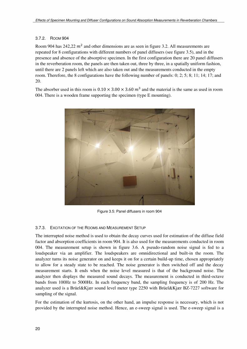
Room 904 has 242,22 and other dimensions are as seen in figure 3.2. All measurements are

repeated for 8 configurations with different numbers of panel diffusers (see figure 3.5), and in the

presence and absence of the absorptive specimen. In the first configuration there are 20 panel diffusers

in the reverberation room, the panels are then taken out, three by three, in a spatially uniform fashion,

until there are 2 panels left which are also taken out and the measurements conducted in the empty

room. Therefore, the 8 configurations have the following number of panels: 0; 2; 5; 8; 11; 14; 17; and

20.

The absorber used in this room is . × . × . and the material is the same as used in room

004. There is a wooden frame supporting the specimen (type E mounting).

Figure 3.5: Panel diffusers in room 904

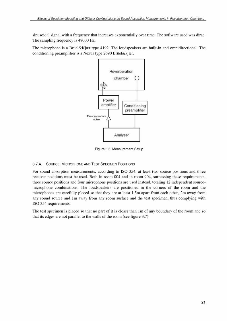
3.7.3. EXCITATION OF THE ROOMS AND MEASUREMENT SETUP

The interrupted noise method is used to obtain the decay curves used for estimation of the diffuse field

factor and absorption coefficients in room 904. It is also used for the measurements conducted in room

004. The measurement setup is shown in figure 3.6. A pseudo-random noise signal is fed to a

loudspeaker via an amplifier. The loudspeakers are omnidirectional and built-in the room. The

analyzer turns its noise generator on and keeps it on for a certain build-up time, chosen appropriately

to allow for a steady state to be reached. The noise generator is then switched off and the decay

measurement starts. It ends when the noise level measured is that of the background noise. The

analyzer then displays the measured sound decays. The measurement is conducted in third-octave

bands from 100Hz to 5000Hz. In each frequency band, the sampling frequency is of 200 Hz. The

analyzer used is a Brüel&Kjær sound level meter type 2250 with Brüel&Kjær BZ-7227 software for

sampling of the signal.

For the estimation of the kurtosis, on the other hand, an impulse response is necessary, which is not

provided by the interrupted noise method. Hence, an e-sweep signal is used. The e-sweep signal is a


21

sinusoidal signal with a frequency that increases exponentially over time. The software used was dirac.

The sampling frequency is 48000 Hz.

The microphone is a Brüel&Kjær type 4192. The loudspeakers are built-in and omnidirectional. The

conditioning preamplifier is a Nexus type 2690 Brüel&kjær.

Figure 3.6: Measurement Setup

3.7.4. SOURCE, MICROPHONE AND TEST SPECIMEN POSITIONS

For sound absorption measurements, according to ISO 354, at least two source positions and three

receiver positions must be used. Both in room 004 and in room 904, surpassing these requirements,

three source positions and four microphone positions are used instead, totaling 12 independent source-

microphone combinations. The loudspeakers are positioned in the corners of the room and the

microphones are carefully placed so that they are at least 1.5m apart from each other, 2m away from

any sound source and 1m away from any room surface and the test specimen, thus complying with

ISO 354 requirements.

The test specimen is placed so that no part of it is closer than 1m of any boundary of the room and so

that its edges are not parallel to the walls of the room (see figure 3.7).


22

Figure 3.7: Source (A, B and C), Microphone (1, 2, 3 and 4) and Test Specimen Positions in room 904.

3.7.5. CLIMATIC CONDITIONS

Variations in climatic conditions can largely influence the measurement results, especially at high

frequencies and low relative humidity [26]. Therefore, in both rooms, the room’s temperature and relative humidity are kept fairly constant throughout all measurements, with a temperature close to

18Cº and a relative humidity of 50% (see figure 3.8).

Figure 3.8: Thermo-hygrometer used to help keep stable climatic conditions


23

4

RESULTS AND DISCUSSION

4.1. DIFFUSE FIELD QUANTIFIERS

4.1.1. HYPOTHESIS

It is here hypothesized that diffusivity increases with a higher number of panel diffusers, if placed

correctly, as previously said. It is also assumed, as previously explained, that absorption by the sample

increases with higher diffusivity. In the light of these assumptions, we expect absorption to increase

with a growing number of panels.

The Sabine absorption coefficient was calculated for different numbers of panel diffusers in the

reverberation room. The results are as follows:

Figure 4.1: Sabine absorption coefficient vs. frequency, in third octave bands, for different number of panel

diffusers, with 95% confidence intervals calculated with the standard deviation that arises from the 12 different

source-microphone positions.


24

Figure 4.2: Sabine absorption coefficient (averaged from 100 to 5000 Hz) vs. number of panels, with the

logarithmic correlation coefficient.

As seen in figure 4.1 the absorption coefficient is markedly lower for the 125 Hz octave band. This

can be explained, on one hand, with the fact that in most reverberation rooms, there is less diffusivity

for lower frequencies, especially if they are below the Schroeder cut-off frequency, as is the 125Hz

octave band. On the other hand, the specimen is a porous absorber, thus it’s not effective in absorbing low frequencies, it is designed to be optimal for higher frequencies. On this account, we would also

expect to see higher absorption for the highest frequency bands. However, this is not the case.

Actually, the 500 Hz octave band is the one with most absorption. This might indicate that the

diffusivity of the room for higher frequencies is also not as good as it should be, thus leading to

underestimated absorption for these frequencies.

Corroborating our hypothesis, the absorption coefficient generally increases with an increasing

number of panel diffusers, with a fairly strong correlation between both (logarithmic =0.98) as seen

in figure 4.2. However, on average, the configuration with 20 panels yields lower values than the one

with 17 panels. This can be explained with the fact that, as mentioned before in this thesis, if the panel

diffusers are not uniformly distributed over space, they will not improve the room’s diffusivity, but can actually decrease it as explained in chapter 2.

4.1.2. DIFFUSE FIELD FACTOR

The hypothesis is that, if the diffuse field factor is a good indicator of the diffuse field conditions, it

should decrease as diffusion increases. Hence, keeping in mind our previously mentioned

assumptions, the diffuse field factor should decrease as the absorption coefficient increases and, in

general, with a growing number of panel diffusers. Actually, it should be lowest for the configuration

that yielded the highest absorption coefficient – the one with 17 panels. Additionally, it should be

lower when the reverberation room is empty than when the absorbing specimen is present, since it is

believed that its presence diminishes diffusion.

The diffuse field factor was calculated both with and without the absorptive sample, for all

configurations with a different number of panels. Focus will be kept mainly on the conditions where

the absorber is present, for that is the most critical condition, i.e. with less diffusivity, and the one


25

where improvements are more necessary. The conditions where the absorber is absent will only be

included for purposes of comparison between absence and presence of absorber.

Figure 4.3: Diffuse field factor vs frequency in third octave bands for different number of panel diffusers.

First of all, it should be mentioned that, as can be seen in figure 4.3, in some cases, e.g. for 5000 kHz

with 11 panels, the diffuse field factor shows as zero. It is not truly zero. This happens because in

formula 3.10 the second component, � ,

, is larger than the first one, � , resulting in a negative � ,

that, when placed in 3.4, yields a non-real solution, a square root of a negative number. Since these

zeros do not represent the real value of the diffuse field factor they were simply discarded in further

results, whenever averages are taken. To prevent this issue more measurement should be taken for

each source-microphone position. Indeed, as previously mentioned in section 3.3, taking only 6

measurements increases the second component of formula 3.10.


26

Figure 4.4: Diffuse field factor vs. number of panel diffusers for different octave bands.

From figure 4.4 it can be seen that the diffuse field factor is generally higher for lower frequencies,

especially for the 125 Hz octave band. This agrees with the observations made before, where the 125

Hz band also corresponded to the lowest absorption. Hence, as hypothesized, a high diffuse field

factor is here potentially indicating low diffusivity. Nonetheless, it should be noted that the 125 Hz

band is below the Schroeder cut-off frequency, where the accuracy of the procedure used to calculate

the diffuse field factor is questionable. The 125 Hz octave band produces some outliers and will not be

included in further analysis, where the arithmetic mean is taken in the third-octave bands centered

from 200 Hz to 5000 Hz.


27

Figure 4.5: Diffuse field factor (averaged from 200 to 5000 Hz) vs. number of panel diffusers in the presence and

absence of the specimen and linear correlation coefficient in the presence of the absorber.

Figure 4.6: Sabine absorption coefficient vs. diffuse field factor (both averaged from 200 to 5000 Hz) for different

number of panel diffusers and linear correlation coefficient.

In the presence of the absorptive specimen, fairly good correlations between the diffuse field factor

and the number of panel diffusers (figure 4.5) and between the diffuse field factor and the absorption

coefficient (figure 4.6) are observed (average from 200 to 5000 Hz). As hypothesized, the diffuse field

factor decreases as the absorption coefficient increases and, in general, with a growing number of

panels. The configuration with 17 panels is the one with the lowest diffuse field factor, corroborating

our hypothesis, since it is also the one with the highest absorption, and so, supposedly, the one with

the highest degree of diffusion. However, the configuration with 5 panels results in slightly lower


28

diffuse field factor values than the configuration with 8 panels. This goes against our hypothesis since

the 8 panel configuration produces higher absorption coefficient.

Also against our hypothesis is the fact that, when comparing the results of absence versus presence of

the absorptive specimen, the diffuse field factor is not lower without the specimen, as it should be if it

were a good indicator, since we assume the room is more diffusive without the absorptive sample.

Additionally, when the specimen is not present, no correlation is found between the diffuse field factor

and the number of panels.

Finally, it should be noted that even if a good correlation is found between the diffuse field factor and

the number of panel diffusers, looking back at figure 4.3 it becomes clear that this correlation is only

true on average, but not for all individual third-octave bands. Indeed, for some frequency bands,

configurations with many panel diffusers have high diffuse field factor values and vice-versa. When

evaluated in third octave bands, the diffuse field factor is not a good indicator and it is not a suitable

tool to fully characterize the diffuse field conditions in a reverberation chamber. And when averaged,

it permits only a rough distinction between poor and satisfactory diffuse field conditions. These

findings agree with what was concluded by Nolan et al. in [19].

4.1.3. KURTOSIS

The hypothesis for kurtosis is the same as for the diffuse field factor: If the kurtosis is a good indicator

of the diffuse field conditions, it should decrease as diffusion increases. Which, keeping in mind our

previously mentioned assumptions, means the kurtosis should decrease as the absorption coefficient

increases and, in general, with a growing number of panel diffusers. It should actually be lowest for

the configuration that yielded the highest absorption coefficient – the one with 17 panels. Additionally,

it should be lower when the reverberation room is empty than when the absorbing specimen is present,

since it is believed that its presence diminishes diffusion.

The Kurtosis was calculated both with and without the absorptive sample, for all configurations with a

different number of panels. The results for the broadband as well as for the 125Hz octave band and the

4000Hz octave band can be seen in figures from 4.7 to 4.12. The results for other frequencies can be

seen in appendix A2.


29

Figure 4.7: � − (left) � − (right) vs. number of panels, from 88 to 5680 Hz and respective linear correlation

coefficients, with 95% confidence intervals calculated with the standard deviation that arises from the 12 different


Figure 4.8: Sabine absorption coefficient vs. � − (left) � − (right) for different number of panel diffusers, from

88 to 5680 Hz and respective linear correlation coefficients.


30

Figure 4.9: � − (left) and � − (right) vs. number of panels, from 2840 to 5680 Hz and respective linear

correlation coefficients, with 95% confidence intervals calculated with the standard deviation that arises from the

12 different source-microphone positions.

Figure 4.10: Sabine absorption coefficient vs. � − (left) � − (right) for different number of panel diffusers,

from 2840 to 5680 Hz and respective linear correlation coefficients.

Figure 4.11: � − (left) � − (right) vs. number of panels, from 88 to 177 Hz and respective linear correlation

coefficients, with 95% confidence intervals calculated with the standard deviation that arises from the 12 different



31

Figure 4.12: Sabine absorption coefficient vs. � − (left) � − (right) for different number of panel diffusers,

from 88 to 177 Hz and respective linear correlation coefficients.

Results show the kurtosis to be well correlated with the absorption coefficient and with the number of

panels for higher frequency bands and for the broadband (88 Hz to 5680 Hz). Agreeing with the

hypothesis, in general, kurtosis decreases as the absorption coefficient and the number of panels

increase, indicating an increase in diffusivity. However, even though this happens in general, many

times with an increase in the number of panels or in the absorption coefficient comes an increase in

kurtosis. This happens with no apparent reason within our assumptions and it goes against our

hypothesis, making the kurtosis only suitable for a rough estimation, since it is not consistent for small

changes. Moreover, these correlations are not found for the low or mid frequency ranges, also

indicating kurtosis as not a very suitable diffusion quantifier.

Within our hypothesis, kurtosis would be expected to be higher (indicating low diffusivity) for lower

frequencies, where there is less diffusivity. However, in general, this is not the case, either for � −

or for � − .

For higher frequencies and for the broadband, when the absorptive specimen is present, the � − is,

on average, slightly higher than when the absorber is not present, indicating lower diffusivity in the

presence of the absorber. For the low and mid frequency ranges and for the � − there are no clear

differences. If the kurtosis was a good indicator of diffusion, higher differences would be expected,

since according to our assumption, the presence of an absorber highly diminishes the diffusivity.

It can be observed that taking the average from 0 to 50 ms produces higher values than taking it from

20 to 80 ms. This is because, in the very beginning of the impulse response, there is direct noise and

stronger, specular reflections which as explained in the chapter 3, leads to higher kurtosis. Related to

this, it is also worth mentioning that the combination where the source and microphone were closer

together yielded higher values, also potentially explained with the direct sound.

Finally, no clear differences between � − and � − are observed that indicate one is more suitable

than the other. Also, it should be noted that none of the correlations and comparisons made before are

statistically significant since there is a high standard deviation among different positions. In itself this

indicates poor diffusivity since it means there is less homogeneity of the diffuse field. Nonetheless, in

general, this standard deviation decreases with the increasing number of panels indicating increasing

diffusivity with an increasing panel number.


32

4.2. MOUNTING CONDITIONS

In a reverberation room, the reverberation times in presence of a porous absorptive sample were

measured under three different mounting conditions: Flush mounting, type A mounting with reflective

boards covering the edges and a mounting similar to the previous one but where the boards have been

removed. The Sabine absorption coefficients were then calculated. In the case without reflective

boards covering the edges, the area of the free edges was added to the area of the horizontal surface,

and the total was used in the calculations.

The results are plotted in figures 4.13 and 4.14.

Figure 4.13: Sabine absorption coefficient in third octave bands for different mounting conditions, with a 95%

confidence interval.

Reflective boards enclosing the free edges of the specimen are required by the ISO 354 standard as

they are expected to minimize sound absorption by the exposed edges, the so called edge effect. And,

indeed, the measurements taken with a mounting without reflective boards yield 6.8 percent higher

absorption coefficients than when using a Type A mounting. This confirms the pertinence of the

requirements in ISO 354.

On average, the absorption coefficient obtained when using the type A mounting is 2.2 percent higher

than when using the flush mounting. A possible explanation is that when the specimen is flush

mounted, we observe a decrease in both the edge effect and the size effect, known causes for the

overestimation of . The edge effect would diminish because the edges would be more effectively

covered, by a denser material - concrete - and with no discontinuities as happens between the room’s floor and the reflective boards, where sound can potentially penetrate. As to the size effect, the

analysis is not so straightforward. Indeed, diffraction at the specimen’s edges occurs because there is a discontinuity. Even when the specimen is flush mounted, there is still a discontinuity. The surface

impedance of concrete is different from that of the specimen, so diffraction occurs, but potentially to a

lesser extent, or in different ways that do not lead to increased absorption.


33

Figure 4.14: Sabine absorption coefficient for different mounting conditions and theoretically estimated absorption

coefficient for third octave bands, with a 95% confidence interval.

The theoretical random incidence absorption coefficient estimated here is size corrected, meaning that

the finiteness of the specimen should not explain the differences observed between theoretical and

measured results, as long as the specimen is flush mounted in an infinite baffle, as assumed by this

theoretical method. With this in mind, it was hypothesized that using a type A mounting, instead of a

flush mounting, could be a cause for the discrepancies between theoretical and measured results,

previously observed in other studies [9]. Corroborating our hypothesis, for higher frequencies, flush

mounting results are closer to theoretical results, than the ones obtained with a type A mounting.

However, for lower frequencies, namely for the 125 Hz and 250 Hz octave bands, the contrary is

observed. Indeed, the theoretical method yields higher values and flush mounting usually originates

lower results than with a type A mounting. Therefore, at least for these frequencies, the mounting

conditions cannot explain the discrepancies between theory and measurements. What can possibly

explain these differences is the lack of diffusivity for low frequencies in the reverberation room, which

leads to the underestimation of the measured coefficients. When in theory, a completely diffuse field is

assumed, thus leading to higher results. Additionally, another factor is causing an overestimation of

the theoretical results, which reach values higher than unity. This factor is thought to be intrinsic to the

expression used to determine the radiation impedance, but further investigation on the matter is

required.


34

5

CONCLUSION AND FUTURE WORK

5.1. DIFFUSE FIELD QUANTIFIERS

In this project, two potential diffuse field quantifiers were measured in reverberation chamber under

eight different configurations: with 0,2,5,8,11,14,17, and 20 panel diffusers. One was the diffuse field

factor, the ratio between the measured standard deviation of the reverberation time and the theoretical

one. The other one, the average kurtosis of an early time-frame of an impulse response, analyzed from

0 to 50 ms and from 20 to 80 ms.

5.1.1. DIFFUSE FIELD FACTOR

In favor of the diffuse field factor, results show that it is generally higher for lower frequencies (where

there is less diffusion); there are good correlations between diffuse field factor and the number of

panel diffusers, and between the diffuse field factor and the Sabine absorption coefficient. On the

other hand, pointing towards the inadequacy of this potential quantifier, diffuse field factor, in the

presence of the absorptive specimen was not higher than in its absence, and the correlations mentioned

before are only true on average, not for all frequency bands. The diffuse field factor appears to be unfit

when evaluated in third octave bands. When averaged it can be used as a rough estimator of the

diffuse field conditions. These conclusions agree with what was previously found by Nolan et al. in

[9].

5.1.2. KURTOSIS

Between the � − and the � − no option is clearly better than the other and neither seem very

suitable as a diffuse field quantifier. When analyzing high frequencies or a broadband response, the

kurtosis does not produce consistent results for small changes but it can be used as a rough estimator;

but, for the low frequency region, where diffusivity is a bigger problem, where improvements are

crucial and a good indicator is more needed, the kurtosis does not seem to be a good quantifier.

Currently there is an ongoing project in DTU where the kurtosis as a diffuse field quantifier is being

analyzed, but there are no previous studies published on the matter, to the extent of the author’s knowledge, and more data is necessary.

Further investigations on other potential indicators of diffusion should be conducted in order to finally

find a suitable diffuse field quantifier, and greatly contribute to increase the low inter-laboratory

reproducibility we observe today.


35

5.2. MOUNTING CONDITIONS

In this study, absorption measurements were conducted under different mounting conditions: a

standard type A mounting and a flush mounting. Results show little differences between both, with

flush mounting yielding, on average, slightly lower absorption coefficients. The measurement results

were also compared with a theoretically estimated random incidence absorption coefficient, calculated

with a size corrected model based on Thomasson’s work [8]. Large differences between theoretical

and measured results were observed for the 125 Hz and 250 Hz octave bands, with the theoretical

values being the highest and the ones obtained with flush mounting being the lowest. For higher

frequencies the differences faded, with type A mounting having slightly higher absorption coefficients,

followed by the flush mounting and the theoretical results.

Results confirm the pertinence of the requirement in ISO 345 of covering the free edges of the

specimen with reflective material. Indeed, complying with this demand clearly reduces the

overestimation of the absorption coefficients. On the other hand, employing flush mounting as a

standard practice, in order to reduce the edge and size effect, does not seem plausible, since it would

constitute yet another requirement on reverberation chambers, one not so easy to accomplish, and with

quite a small impact.

As for the differences between the theoretically estimated coefficients and the measured Sabine

coefficients, results lead to believe mounting conditions are not a major factor. Not only because both

mounting conditions lead to similar results, but also because, for lower frequencies, coefficients

obtained with a flush mounting are even more distanced from the theoretical ones than when using a

type A mounting.


36


37

BIBLIOGRAPHY

[1] Cheol-Ho Jeong. Absorption and impedance boundary conditions for phased geometrical-

acoustics methods. The Journal of the Acoustical Society of America, 132(4):2347–2358, 2012.

[2] Iso. ISO 354 Acoustics–Measurement of sound absorption in a reverberation room, 2003.

[3] MLS Vercammen. Improving the accuracy of sound absorption measurement according to iso

354. In Proc. of the International Symposium on Room Acoustics, pages 1–4, 2010.

[4] David, T Bradley, Markus Müller-Trapet, Jacob Adelgren, and Michael Vorländer. Effect of

boundary diffusers in a reverberation chamber: Standardized diffuse field quantifiersa). The

Journal of the Acoustical Society of America, 135(4):1898–1906, 2014.

[5] Margriet, R Lautenbach and Martijn L Vercammen. Can we use the standard deviation of the

reverberation time to describe diffusion in a reverberation chamber? In Proceedings of Meetings

on Acoustics, volume 19, page 015054. Acoustical Society of America, 2013.

[6] A De Bruijn. A mathematical analysis concerning the edge effect of sound absorbing materials.

Acta Acustica united with Acustica, 28(1):33–44, 1973.

[7] Thomas W Bartel. Effect of absorber geometry on apparent absorption coefficients as measured

in a reverberation chamber. The Journal of the Acoustical Society of America, 69(4):1065–1074,

1981.

[8] S-I Thomasson. On the absorption coefficient. Acta Acustica united with Acustica, 44(4):265–273, 1980.

[9] Melanie Nolan, Cheol-Ho Jeong, Jonas Brunskog, Julia Rodenas, Fabien Chevillotte, and Luc

Jaouen. Different radiation impedance models for finite porous materials. EuroNoise 2015.

[10] A. P. Oliveira de Carvalho. Acústica Ambiental e de Edifícios. FEUP, Porto, 8.8 edition, 2014.

[11] UNEEN ISO. 10534-1: 2002. Acoustics. Determination of sound absorption coefficient and

impedance in impedance tubes, Part, 1.

[12] BSEN ISO. 10534-2: 2001. Acoustics. Determination of sound absorption coefficient and

impedance in impedance tubes. Transfer-function method. Geneve, 2001.

[13] Frederick Alton Everest, Ken C Pohlmann, and Tab Books. The master handbook of acoustics,

volume 4. McGraw-Hill New York, 2001.

[14] M Vercammen. The effectiveness of diffusers by determining the sound absorption in the

reverberation room, 1997.

[15] A de Bruijn. The edge effect of sound absorbing materials “revisited”, 2007.

[16] ASTM Standard. C423-09a. Standard Test Method for Sound Absorption and Sound Absorption

Coefficients by the Reverberation Room Method, 2009.

[17] ASTM Standard. E90, 2009,“standard test method for laboratory measurement of airborne sound

transmission loss of building partitions and elements,” astm international, west conshohocken, pa, 2010, doi: 10.1520/e0090-09.

[18] Mélanie Nolan, Martijn Vercammen, Cheol-Ho Jeong, and Jonas Brunskog. The use of a

reference absorber for absorption measurements in a reverberation chamber. In 7th Forum

Acusticum.


38

[19] Melanie Nolan, Martijn Vercammen, and Cheol-Ho Jeong. Effects of different diffuser types on

the diffusivity in reverberation chambers. EuroNoise 2015, 2015.

[20] John, L Davy, IP Dunn, and P Dubout. The variance of decay rates in reverberation rooms. Acta

Acustica united with Acustica, 43(1):12–25, 1979.

[21] http://se.mathworks.com/help/symbolic/mupad_ref/stats-kurtosis.html?refresh=true, Accessed on

10-10-2015.

[22] Jonathan, S Abel and Patty Huang. A simple, robust measure of reverberation echo density. In

Audio Engineering Society Convention 121. Audio Engineering Society, 2006.

[23] Kuttruff, H. Room Acoustics. Fifth edition, CRC Press, 2009

[24] Keith Attenborough. Acoustical characteristics of porous materials. Physics reports, 82(3):179–227, 1982.

[25] Miki, Y. Acoustical properties of porous materials modifications of Delany-Bazly models, J.

Accoust Soc. Japan 11 19-28 1990.

[26] DIN ISO. 9613–1: 1993. acoustics. attenuation of sound during propagation outdoors. part 1:

Calculation of the absorption of sound by the atmosphere. International Organization for

Standardization, Geneva, 1993.

http://se.mathworks.com/help/symbolic/mupad_ref/stats-kurtosis.html?refresh=true


i

APPENDIX A

Figure A.1: �0−50(left) �20−80 (right) vs number of panels, from 177 to 355 Hz and respective linear correlation

coefficients, with 95% confidence intervals.

Figure A.2:Sabine absorption coefficient vs �0−50(left) �20−80 (right) for different number of panel diffusers, from



ii








iii








iv

Figure A.9: Radiation impedance - Reference Table

E FFECTS OF S PECIMEN M OUNTING - Repositório … FFECTS OF S PECIMEN M OUNTING AND D IFFUSER C...

Documents

Transcript of E FFECTS OF S PECIMEN M OUNTING - Repositório … FFECTS OF S PECIMEN M OUNTING AND D IFFUSER C...