
fileINSTITUTO DE PESQUISAS ENERGÉTICAS E NUCLEARES Autarquia associada à Universidade de São...
128
# $ %& ’(%) * &+ &(%& % &&’%& (,- .’/(&( * +()+ & 0.+-&+- 0( (, 1%. %& .’ & 23((& 0&%4 3 3& ’ (5%.( % 6 .%)( 3. & (%&7 *8 8 "9( :(-; 3 <=>
Transcript of fileINSTITUTO DE PESQUISAS ENERGÉTICAS E NUCLEARES Autarquia associada à Universidade de São...
�
�
� ���# �������������$� ������������������ ���
��%&��������'�����(%)��*�&+����&(�%&��%��&���&'�%&����(,��-�.�'���/(&(���*���+()+��������&��0��.+-&+����-��
��0�(�����(,��1�%��.��
� ����� ������%&���� .�'�� ���&�� ������23(�(&��� ����� �0&�%4��� ��� ���3� �����3&��� �'� �(5%.(��� %�� 6���������.%���)(���3.����������&������
� ��(�%&����7�
� ���*8���8��"9�(��:��(-�;�
������3���
<=>��
INSTITUTO DE PESQUISAS ENERGÉTICAS E NUCLEARES
Autarquia associada à Universidade de São Paulo
AND
MAASTRICHT UNIVERSITY
Monte Carlo modelling of the patient and treatment delivery complexities for high dose rate brachytherapy
Gabriel Paiva Fonseca
Thesis to obtain the degree of Doctor at
Maastricht University, in accordance with
the decision of the Board of Deans, and at
Universidade de São Paulo in the field of
“Ciências na Área de Tecnologia Nuclear –
Reatores”.
Supervisors:
Dr. Hélio Yoriyaz
Dr. Frank Verhaegen
Dr. Brigitte Reniers
Versão Corrigida
Versão original disponível no IPEN
São Paulo / Maastricht
2015

Supervisors
Prof. Dr. Frank Verhaegen
Prof. Dr. Hélio Yoriyaz
Co-supervisor
Dr. Brigitte Reniers
Assessment Committee – the Netherlands
Prof. Dr. Philip Lambin (chairman), Maastricht University
Prof. Dr. Dietmar Georg, Medical University Vienna
Prof. Dr. Luc Beaulieu, University Laval, Quebec City, Canada
Dr. Ans Swinnen, Maastro Clinic
Dr. Ludy Lutgens, Maastro Clinic
Assessment Committee – Brazil
Prof. Dr. Hélio Yoriyaz (chairman), Instituto de Pesquisas Energéticas e Nucleares
Prof. Dr. Laura Natal Rodrigues, Universidade de São Paulo
Prof. Dr. Marcelo Baptista de Freitas, Universidade Federal de São Paulo
Prof. Dr. Elisabeth Mateus Yoshimura, Universidade de São Paulo
These studies were funded by a PhD Scholarship from Fundação de Amparo à Pesquisa do
Estado de São Paulo (FAPESP, SP, Brazil).

This thesis is dedicated to my beloved
wife, Louise, for her support during the
most difficult moments, for being part of
my happiest memories and for everything
that we are going to experience together.
Acknowledgments
Foremost, I would like to acknowledge my supervisors Prof. Dr. Hélio Yoriyaz, Prof.
Dr. Frank Verhaegen and Dr. Brigitte Reniers for the opportunity, patience and dedication
that without doubts were essential for this thesis and very important for my personal life.
Hélio, thank you for accept me as your student back in 2004, during my master and
Ph.D. This experience greatly improved my formation and guided me into the scientific
career. Thanks for teach and work with me (even during your holidays) and for many
pleasant moments.
Frank, thank you for providing me the opportunity to study in Europe and be part of
your research team. I cannot describe how fortunate I was for being so well received and how
it changed my perception of the world. Many thanks for the uncountable times you had to
read my papers and for always (even being the busiest person I know) find time to teach and
guide me.
Brigitte, thank you for find time to contribute with this thesis, for the innumerous and
productive discussions and for being available even to visit different hospitals seeking for
data that were very important.
This Ph.D would not be possible without a person who was part of my professional
life only for a short period, but made very important contributions suggesting the subject of
my master thesis and introducing me to Frank. Thank you Dr. Esmeralda Poli.
Guillaume, Mark and Shane, work with you was very important and I owe you a lot
for it.
I had a terrific experience in the Netherlands and I owe it to you guys: Shane, Mark,
Aniek, Ruud, Guillaume, Sean, Patrick, Raghu, Skadi, Karen, Sara, Ralph, Stefan, Davide,
Daniela, Lucas, Evelyn, Emmanuel, Isabel, Lotte, Pedro, Ruben, Jurgen and Timo. Thanks
for the laughs, runs, dinner, squash games (sorry for the bruises and scars) and for all the
help.
Thanks to the whole radiotherapy team in Brazil, in particular to Gabriela, Rodrigo
and Camila, for the discussions and experiments late night or during the weekends. Your
contribution was very important and I hope we can keep working together.
I would like to thank my colleagues and friends in Brazil for the support, laughs,
barbecues and especially for all the time you kept me out of the office. It did not contribute

much with my work, but gave me a lot of pleasant moments and good memories. Thank you
guys; Paula, Gregório, Arthur, Cesar, Henrique, Carlos, Tassio, Rodrigo, Felipe, Talita, Yan,
Michele, Murillo.
Thank you Louise for being with me all the time since 2002 and for your importance
in my life. Your determination kept me on track and helped me to pursue my goals.
Finally, I would like to thank my beloved parents, Carlos e Madalena, my brother
Rodrigo and my sisters Roberta e Juliana. I am thankful for being part of this family. The
distance was tough, but your strength and love allowed me to keep going.
* The financial support provide by FAPESP was crucial to the development of this work.
** AMIGOBrachy uses icons downloaded from www.flaticon.com and www.freepik.com
(free license with attribution) and made by: Sarfraz Shoukat, Nice and serious, FreePic,
Yannick, Simplelcon, PICOL, Situ-Herrera,Vectorgraphit, Catalin Fertu, Anton Saputro,
Icon Works, Pavel Kozlov and Fermam Aziz. More information are available in the
software user guide.
i
Abstract
Brachytherapy treatments are commonly performed using the American Association of
Physicists in Medicine (AAPM) Task Group report TG-43U1 absorbed dose to water
formalism, which neglects human tissue densities, material compositions, body interfaces,
body shape and dose perturbations from applicators. The significance of these effects has
been described by the AAPM Task Group report TG-186 in published guidelines towards the
implementation of Treatment Planning Systems (TPS) which can take into account the above
mentioned complexities. This departure from the water kernel based dose calculation
approach requires relevant scientific efforts in several fields. This thesis aims to improve
brachytherapy treatment planning accuracy following TG-186 recommendations and going
beyond it. A software has been developed to integrate clinical treatment plans with Monte
Carlo (MC) simulations; high fidelity CAD-Mesh geometry was employed to improve
brachytherapy applicators modelling; different dose report quantities, Dw,m (dose to water in
medium) and Dm,m (dose to medium in medium), were obtained for a head and neck case
using small cavity theory (SCT) and large cavity theory (LCT); the dose component due to
the source moving within the patient was evaluated for gynecological and prostate clinical
cases using speed profiles from the literature. Moreover, source speed measurements were
performed using a high speed camera. Dose calculations using MC showed overdosing
around 5% within the target volume for a gynecological case comparing results obtained
including tissue, air and applicator effects against a homogeneous water phantom. On the
other hand, the same comparison showed underdosing around 5% when including tissue and
air composition for an interstitial arm case. A hollow cylinder applicator was responsible for
the overdosing observed for the gynecological case highlighting the importance of accurate
applicator modelling. The evaluated CAD-Mesh applicators models included a Fletcher-
Williamson shielded applicator and a deformable balloon used for accelerated partial breast
irradiation. Results obtained were equivalent to ones obtained with conventional constructive
solid geometry and may be convenient for complex applicators and/or when manufacturer
CAD models are available. Differences between Dm,m and Dw,m (SCT or LCT) are up to 14%
for bone in a evaluated head and neck case. The approach (SCT or LCT) leads to differences
up to 28% for bone and 36% for teeth. Differences can also be significant due to the source
movement since some speed profiles from literature show low source speeds or uniform
accelerated movements. Considering the worst case scenario and without include any dwell
time correction, the transit dose can reach 3% of the prescribed dose in a gynecological case
with 4 catheters and up to 11.1% when comparing the average prostate dose for a case with
16 catheters. The transit dose for a high speed (measured with a video camera) source is not
uniformly distributed leading to over and underdosing, which is within 1.4% for commonly
prescribed doses (3–10 Gy). The main subjects evaluated in this thesis are relevant for
brachytherapy treatment planning and can improve treatment accuracy. Many of the issues
described in here can be assessed with the software, coupled with a MC code, developed in
this work.
Key words: Brachytherapy, Monte Carlo, HDR 192
Ir, MBDCA
ii
Resumo
Tratamentos braquiterápicos são comumente realizados conforme o relatório da American
Association of Physicists in Medicine (AAPM), Task Group report TG-43U1, o qual define o
formalismo para cálculo de dose absorvida na água e não considera a composição dos
materiais, densidades, dimensões do paciente e o efeito dos aplicadores. Estes efeitos podem
ser significantes, conforme descrito pelo recente relatório da AAPM, Task Group report TG-
186, que define diretrizes para que sistemas de planejamento modernos, capazes de
considerar as complexidades descritas acima, sejam implementados. Esta tese tem como
objetivo contribuir para o aumento da exatidão dos planejamentos de tratamento
braquiterápicos, seguindo as recomendações do TG-186 e indo além do mesmo. Um software
foi desenvolvido para integrar planejamentos de tratamento e simulações pelo método de
Monte Carlo (MC); modelos acurados, CAD-Mesh, foram utilizados para representar
aplicadores braquiterápicos; Grandezas utilizadas para reportar dose absorvida, Dw,m (dose
para água no meio) e Dm,m (dose para o meio no meio), foram calculadas para um tratamento
de cabeça e pescoço, considerando a teoria para pequenas (SCT – small cavity theory) e
grandes cavidades (LCT – large cavity theory); a componente da dose em razão do
movimento da fonte foi avaliada para tratamentos de próstata e ginecológicos. Perfis de
velocidade obtidos na literatura foram utilizados; medidas de velocidade de uma fonte
braquiterapica foram realizadas com uma câmera de alta taxa de aquisição. Cálculos de dose
obtidos usando MC (incluindo a composição e densidade dos tecidos, ar e o aplicador)
mostram sobredoses de aproximadamente 5% dentro do volume alvo, em um tratamento
ginecológico, quando comparados aos resultados obtidos com um meio homogêneo de água.
Por sua vez, subdoses de aproximadamente 5% foram observadas ao considerar a composição
dos tecidos e regiões com ar em um tratamento intersticial de braço. Um aplicador cilíndrico
oco resultou na sobredose observada no caso ginecológico, ressaltando a necessidade de
modelos acurados para representar os aplicadores. Os modelos CAD-Mesh utilizados incluem
um aplicador Fletcher-Williamson, com blindagem, e um balão deformável para irradiação de
mama. Os resultados obtidos com estes modelos são equivalentes aos obtidos com modelos
geométricos convencionais. Este recurso pode ser conveniente para aplicadores complexos
e/ou quando o projeto dos aplicadores for disponibilizado pelo fabricante. Cálculos de dose,
com a composição real dos tecidos humanos, podem apresentar diferenças significativas em
razão da grandeza adotada. Diferenças entre Dm,m e Dw,m (SCT ou LCT) chegam a 14% em
razão da composição do osso. A metodologia adotada (SCT ou LCT) resulta em diferenças de
até 28% para o osso e 36% para os dentes. A componente de dose de trânsito também pode
levar a diferenças significativas, uma vez que baixas velocidades ou movimentos
uniformemente acelerados foram descritos na literatura. Considerando a pior condição e sem
incluir nenhuma correção no tempo de parada, a dose de trânsito pode chegar a 3% da dose
prescrita para um caso ginecológico, com 4 cateteres, e até 11.1% da dose prescrita para um
tratamento de próstata, com 16 cateteres. A dose de trânsito para a fonte avaliada (velocidade
obtida experimentalmente) não é uniformemente distribuída e pode levar a sub ou sobredoses
de até 1.4% das doses comumente prescritas (3–10 Gy). Os tópicos estudados são relevantes
para tratamentos braquiterápicos e podem contribuir para o aumento de sua acurácia. Os
efeitos estudados podem ser avaliados com o uso do software, associado a um código MC,
desenvolvido.
Palavras chave: Braquiterapia, Monte Carlo, HDR 192
Ir, MBDCA

iii
Summary
1 INTRODUCTION ................................................................................................................. 2
1.1 AMIGOBrachy ............................................................................................................... 3
1.2 CAD-Mesh....................................................................................................................... 3
1.3 Dose specification ........................................................................................................... 4
1.4 Transit dose ..................................................................................................................... 6
1.5 Speed Measurements...................................................................................................... 8
2 OBJECTIVES ...................................................................................................................... 10
3 LITERATURE REVIEW ................................................................................................... 12
3.1 Brachytherapy history and current practice ............................................................. 12
3.2 MC methods in brachytherapy ................................................................................... 19
4 MATERIALS AND METHODS ........................................................................................ 23
4.1 Monte Carlo codes ........................................................................................................ 23
4.2 AMIGOBrachy ............................................................................................................. 25
4.3 CAD-Mesh..................................................................................................................... 30
4.4 Dose specification (Dw,m and Dm,m) .............................................................................. 37
4.5 Transit dose ................................................................................................................... 39
4.6 Speed measurements .................................................................................................... 46
5 RESULTS AND DISCUSSIONS ........................................................................................ 50
5.1 AMIGOBrachy ............................................................................................................. 50
5.2 CAD-Mesh..................................................................................................................... 54
5.3 Dose specification ......................................................................................................... 61
5.4 Transit dose ................................................................................................................... 71
5.5 Speed measurements .................................................................................................... 78
6 CONCLUSIONS .................................................................................................................. 85
7 FUTURE PERSPECTIVES ................................................................................................ 88
iv
8 LIST OF PUBLICATIONS ................................................................................................ 91
8.1 Published articles.......................................................................................................... 91
8.2 Conferences ................................................................................................................... 92
9 CURRICULUM VITAE ..................................................................................................... 94
10 REFERENCES..................................................................................................................... 96
11 VALORIZATION ADDENDUM ..................................................................................... 107
11.1 Innovation ................................................................................................................... 107
11.2 Clinical relevance ....................................................................................................... 109
11.3 Societal relevance ....................................................................................................... 109
11.4 Commercial relevance................................................................................................ 110
v
Figure List
Figure 1. a) mass energy absorption coefficients (µ en/) of various human tissues relative to
water coefficients. Values for elemental media obtained from NIST39
and combined into
human tissues using the mass-fraction of each element. b) Unrestricted mass collision
stopping power /� ratios of various human tissues relative to those for water. Values
obtained using ESTAR database considering the mass-fraction of each element.40
.................. 6
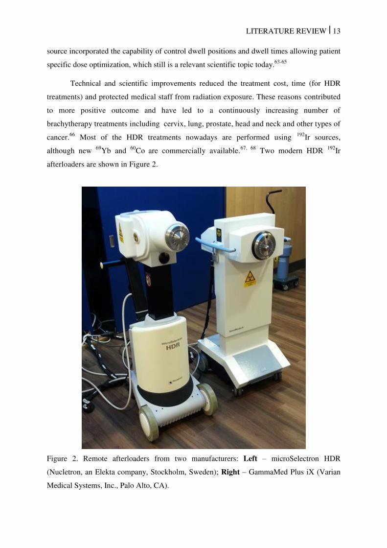
Figure 2. Remote afterloaders from two manufacturers: Left – microSelectron HDR
(Nucletron, an Elekta company, Stockholm, Sweden); Right – GammaMed Plus iX (Varian
Medical Systems, Inc., Palo Alto, CA). .................................................................................... 13
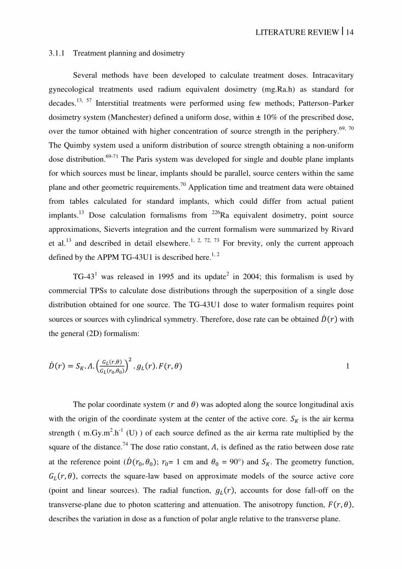
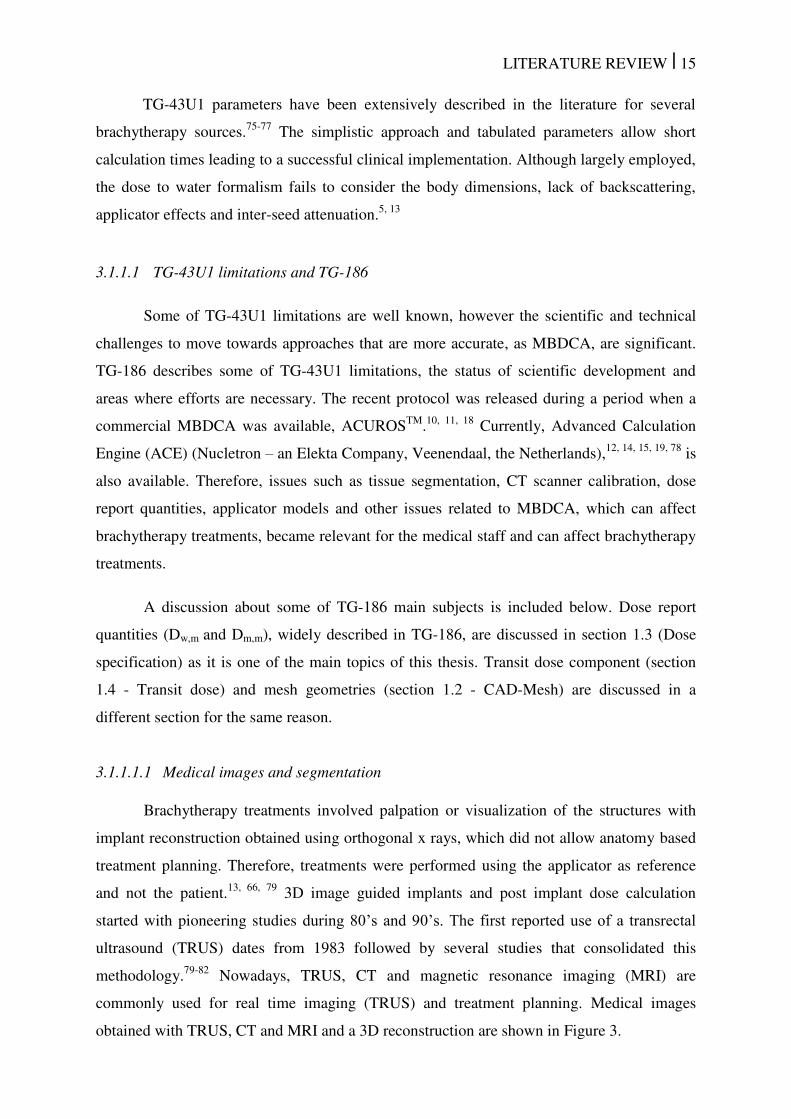
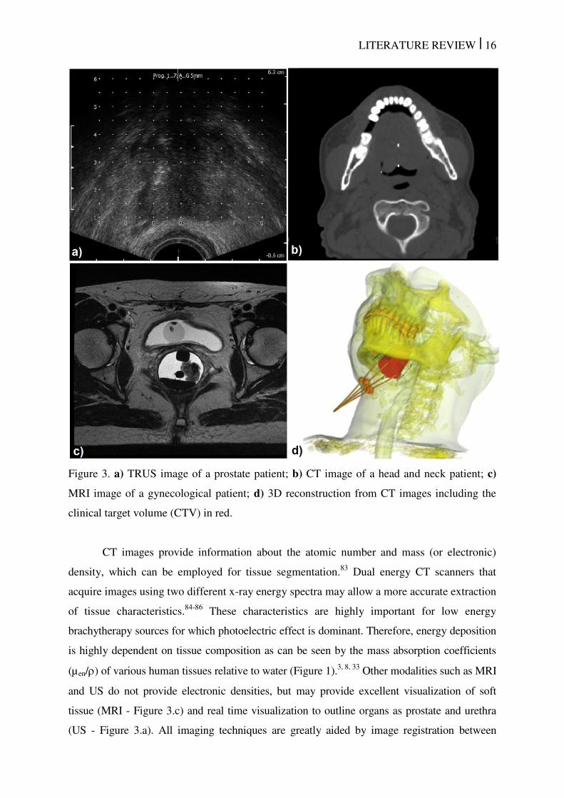
Figure 3. a) TRUS image of a prostate patient; b) CT image of a head and neck patient; c)
MRI image of a gynecological patient; d) 3D reconstruction from CT images including the
clinical target volume (CTV) in red. ......................................................................................... 16
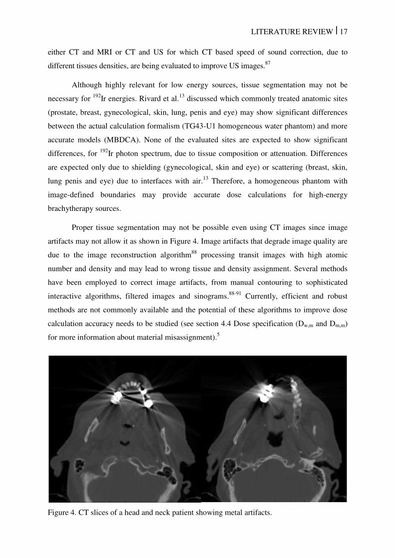
Figure 4. CT slices of a head and neck patient showing metal artifacts. .................................. 17
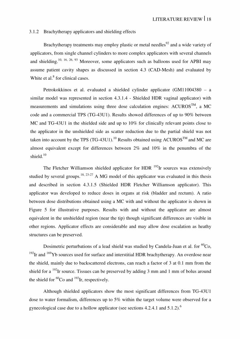
Figure 5. Ratio between dose distributions obtained with MC with and without including the
Fletcher Williamson applicator. The dark blue region represents the applicator. .................... 19
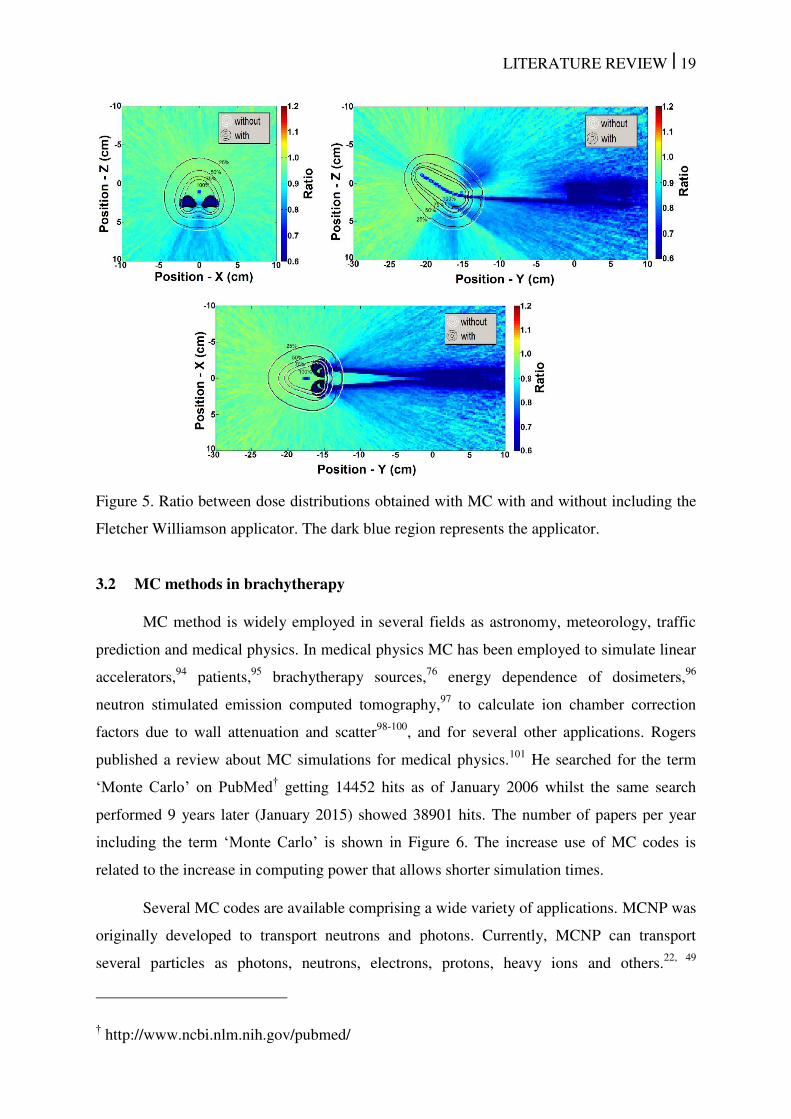
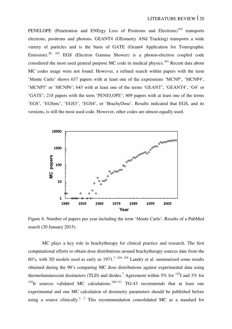
Figure 6. Number of papers per year including the term ‘Monte Carlo’. Results of a PubMed
search (20 January 2015). ......................................................................................................... 20
Figure 7. Flowchart with AMIGOBrachy’s main functionalities, which are described in the
user-guide. The process starts with importing or creating a DICOM sequence of images,
followed by defining the simulation parameters and initiating MCNP6, and finishes by
importing and analyzing the simulated dose distributions. ....................................................... 26
Figure 8. A 180º tungsten shielded applicator modeled using: a) analytical geometry; b)
(1x1x1) mm3 voxels; c) mesh structures created with Abaqus
TM. The dimensions are based on
the GM11004380 applicator (Varian Medical Systems) and on the ACUROSTM
applicator
database. .................................................................................................................................... 27
Figure 9. A sequence of images used by AMIGOBrachy: a) importing the DICOM patient
CT image; b) defining structures by importing DICOM contours (e.g. the highlighted bone
contours); c) defining the material map (using HU numbers or drawing tools), which consists
of air (black region), adipose tissue (blue region), muscle (green region) and bone (yellow
region); d) defining the voxel phantom region (external rectangle) and the dose scoring
region (internal rectangle). ........................................................................................................ 29
Figure 10. Example MG for the idealized APBI applicator showing the external surface and
an inner section using a cutaway plane. The wall material is barium loaded polymer. ............ 32
vi
Figure 11. a) Axial CT image of an APBI balloon applicator inserted in a post surgical breast
cavity. The wall is clearly visible due to barium loading. The EBS channel is occupied by a
dummy insert to identify dwell positions. The balloon is filled with a saline solution. The
high intensity pixels correspond to the end cap. Neither saline solution nor end cap are
modeled in this thesis. b) MG for the APBI applicator showing the external surface. ............ 33
Figure 12. Schematic representation of the shielded cylindrical vaginal applicator. ............... 34
Figure 13. CAD representation of the Fletcher Williamson applicator (from AbaqusTM
). ...... 35
Figure 14. Axial and sagittal view of the evaluated head and neck clinical case. The numbers
indicate voxels positions where the photon spectrum was scored. Green arrows and squares
were added to show the catheter positions (five of the six catheters can be visualized). ......... 37
Figure 15. a) Source moving between three dwell positions with inter-dwell distance of 0.5
cm. b) Source speed profile for a uniform accelerated movement. c) Contribution of each
source position to transit dose at the reference point due the source traveling between the
dwell positions and returning to the safe. ................................................................................. 42
Figure 16. Experimental setup for source speed measurements. The insert (top-right) was
obtained from one of the acquired slow motion videos. The source guide was positioned to be
clinically relevant avoiding excessive bending during the experiments. .................................. 46
Figure 17. AMIGOBrachy screenshots of a) AMIGOBrachy ImageView module; b) 3D
rendering of lungs; c) dose distribution of a single source dwell position with dose profiles; d)
dose distribution obtained using a titanium fletcher applicator and a sequence of source dwell
positions. ................................................................................................................................... 50
Figure 18. Results for the two patient geometries: the intracavitary gynecological case (left
panels) and the interstitial arm case (right panels). a) 3D view indicating the assigned
materials. b) Isodoses and dose ratio ACUROSTM
/MCNP6. c) Isodoses and dose ratio
MCNP6(homogeneous water)/MCNP6(heterogeneous geometry). ......................................... 53
Figure 19. Calculation times in seconds for simulating 107 primary photons from an
192Ir
source in a water cube represented by a MG with varying number of volume elements. ........ 55
Figure 20. (a) Inside the balloon wall there appears to be a lack of backscatter from the
balloon wall and the water beyond it in the MG case. (b) However, the photon spectra
directly outside the balloon agree between MG and CSG. ....................................................... 55
Figure 21. a) Dose ratio in an axial slice intersecting the origin from dose distributions
obtained with MG and CSG representations of the idealized APBI balloon applicator using
Geant4 and a 50 kV photon spectrum. Isodose lines are also presented. b) Dose ratio obtained
using MG in Geant4 and MCNP6. Dose in the balloon wall was not scored in Geant4 hence
vii
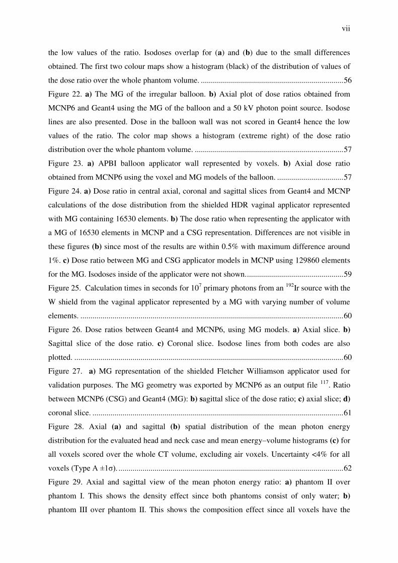
the low values of the ratio. Isodoses overlap for (a) and (b) due to the small differences
obtained. The first two colour maps show a histogram (black) of the distribution of values of
the dose ratio over the whole phantom volume. ....................................................................... 56
Figure 22. a) The MG of the irregular balloon. b) Axial plot of dose ratios obtained from
MCNP6 and Geant4 using the MG of the balloon and a 50 kV photon point source. Isodose
lines are also presented. Dose in the balloon wall was not scored in Geant4 hence the low
values of the ratio. The color map shows a histogram (extreme right) of the dose ratio
distribution over the whole phantom volume. .......................................................................... 57
Figure 23. a) APBI balloon applicator wall represented by voxels. b) Axial dose ratio
obtained from MCNP6 using the voxel and MG models of the balloon. ................................. 57
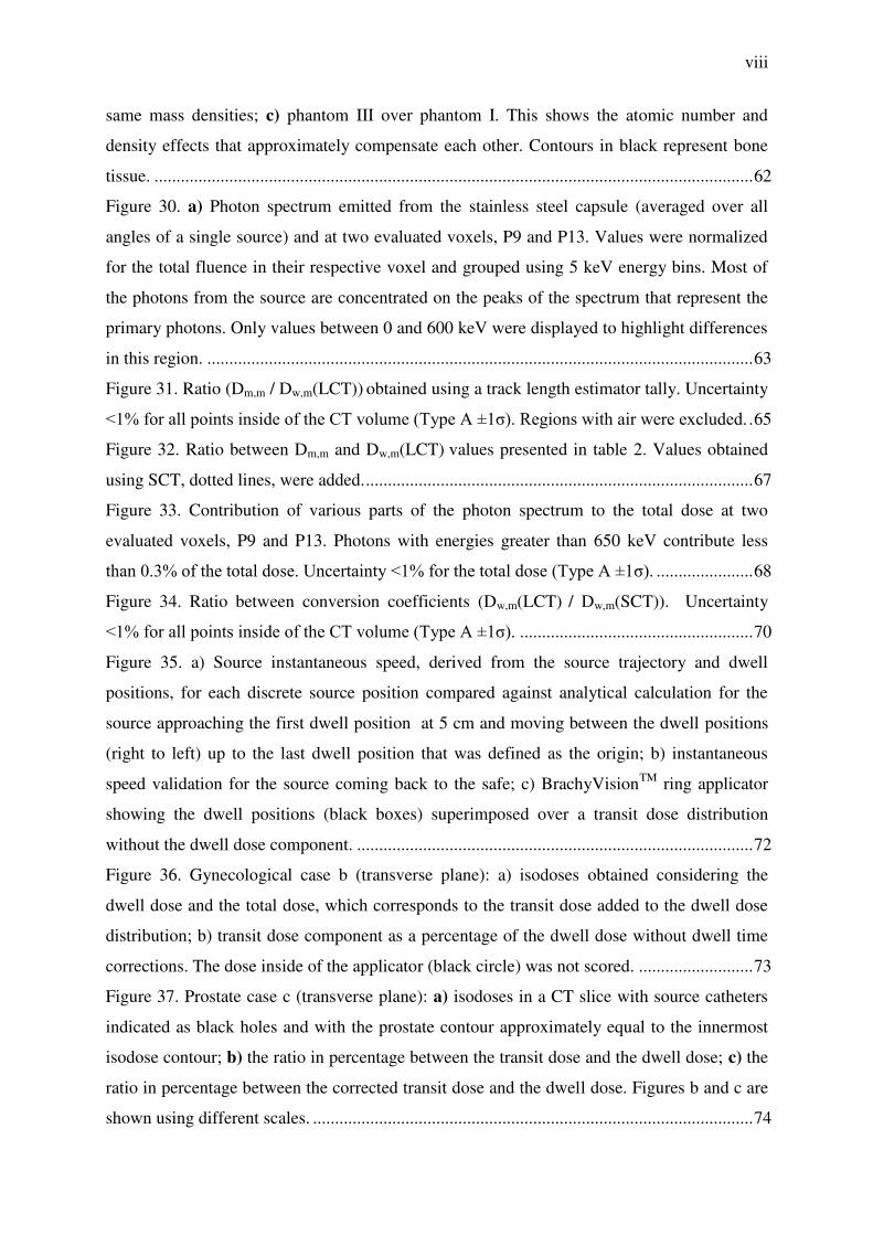
Figure 24. a) Dose ratio in central axial, coronal and sagittal slices from Geant4 and MCNP
calculations of the dose distribution from the shielded HDR vaginal applicator represented
with MG containing 16530 elements. b) The dose ratio when representing the applicator with
a MG of 16530 elements in MCNP and a CSG representation. Differences are not visible in
these figures (b) since most of the results are within 0.5% with maximum difference around
1%. c) Dose ratio between MG and CSG applicator models in MCNP using 129860 elements
for the MG. Isodoses inside of the applicator were not shown. ................................................ 59
Figure 25. Calculation times in seconds for 107 primary photons from an
192Ir source with the
W shield from the vaginal applicator represented by a MG with varying number of volume
elements. ................................................................................................................................... 60
Figure 26. Dose ratios between Geant4 and MCNP6, using MG models. a) Axial slice. b)
Sagittal slice of the dose ratio. c) Coronal slice. Isodose lines from both codes are also
plotted. ...................................................................................................................................... 60
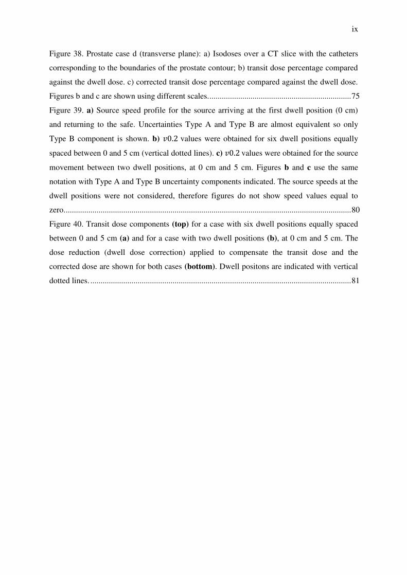
Figure 27. a) MG representation of the shielded Fletcher Williamson applicator used for
validation purposes. The MG geometry was exported by MCNP6 as an output file 117
. Ratio
between MCNP6 (CSG) and Geant4 (MG): b) sagittal slice of the dose ratio; c) axial slice; d)
coronal slice. ............................................................................................................................. 61
Figure 28. Axial (a) and sagittal (b) spatial distribution of the mean photon energy
distribution for the evaluated head and neck case and mean energy–volume histograms (c) for
all voxels scored over the whole CT volume, excluding air voxels. Uncertainty <4% for all
voxels (Type A ±1σ). ................................................................................................................ 62
Figure 29. Axial and sagittal view of the mean photon energy ratio: a) phantom II over
phantom I. This shows the density effect since both phantoms consist of only water; b)
phantom III over phantom II. This shows the composition effect since all voxels have the
viii
same mass densities; c) phantom III over phantom I. This shows the atomic number and
density effects that approximately compensate each other. Contours in black represent bone
tissue. ........................................................................................................................................ 62
Figure 30. a) Photon spectrum emitted from the stainless steel capsule (averaged over all
angles of a single source) and at two evaluated voxels, P9 and P13. Values were normalized
for the total fluence in their respective voxel and grouped using 5 keV energy bins. Most of
the photons from the source are concentrated on the peaks of the spectrum that represent the
primary photons. Only values between 0 and 600 keV were displayed to highlight differences
in this region. ............................................................................................................................ 63
Figure 31. Ratio (Dm,m / Dw,m(LCT)) obtained using a track length estimator tally. Uncertainty
<1% for all points inside of the CT volume (Type A ±1σ). Regions with air were excluded. . 65
Figure 32. Ratio between Dm,m and Dw,m(LCT) values presented in table 2. Values obtained
using SCT, dotted lines, were added. ........................................................................................ 67
Figure 33. Contribution of various parts of the photon spectrum to the total dose at two
evaluated voxels, P9 and P13. Photons with energies greater than 650 keV contribute less
than 0.3% of the total dose. Uncertainty <1% for the total dose (Type A ±1σ). ...................... 68
Figure 34. Ratio between conversion coefficients (Dw,m(LCT) / Dw,m(SCT)). Uncertainty
<1% for all points inside of the CT volume (Type A ±1σ). ..................................................... 70
Figure 35. a) Source instantaneous speed, derived from the source trajectory and dwell
positions, for each discrete source position compared against analytical calculation for the
source approaching the first dwell position at 5 cm and moving between the dwell positions
(right to left) up to the last dwell position that was defined as the origin; b) instantaneous
speed validation for the source coming back to the safe; c) BrachyVisionTM
ring applicator
showing the dwell positions (black boxes) superimposed over a transit dose distribution
without the dwell dose component. .......................................................................................... 72
Figure 36. Gynecological case b (transverse plane): a) isodoses obtained considering the
dwell dose and the total dose, which corresponds to the transit dose added to the dwell dose
distribution; b) transit dose component as a percentage of the dwell dose without dwell time
corrections. The dose inside of the applicator (black circle) was not scored. .......................... 73
Figure 37. Prostate case c (transverse plane): a) isodoses in a CT slice with source catheters
indicated as black holes and with the prostate contour approximately equal to the innermost
isodose contour; b) the ratio in percentage between the transit dose and the dwell dose; c) the
ratio in percentage between the corrected transit dose and the dwell dose. Figures b and c are
shown using different scales. .................................................................................................... 74
ix
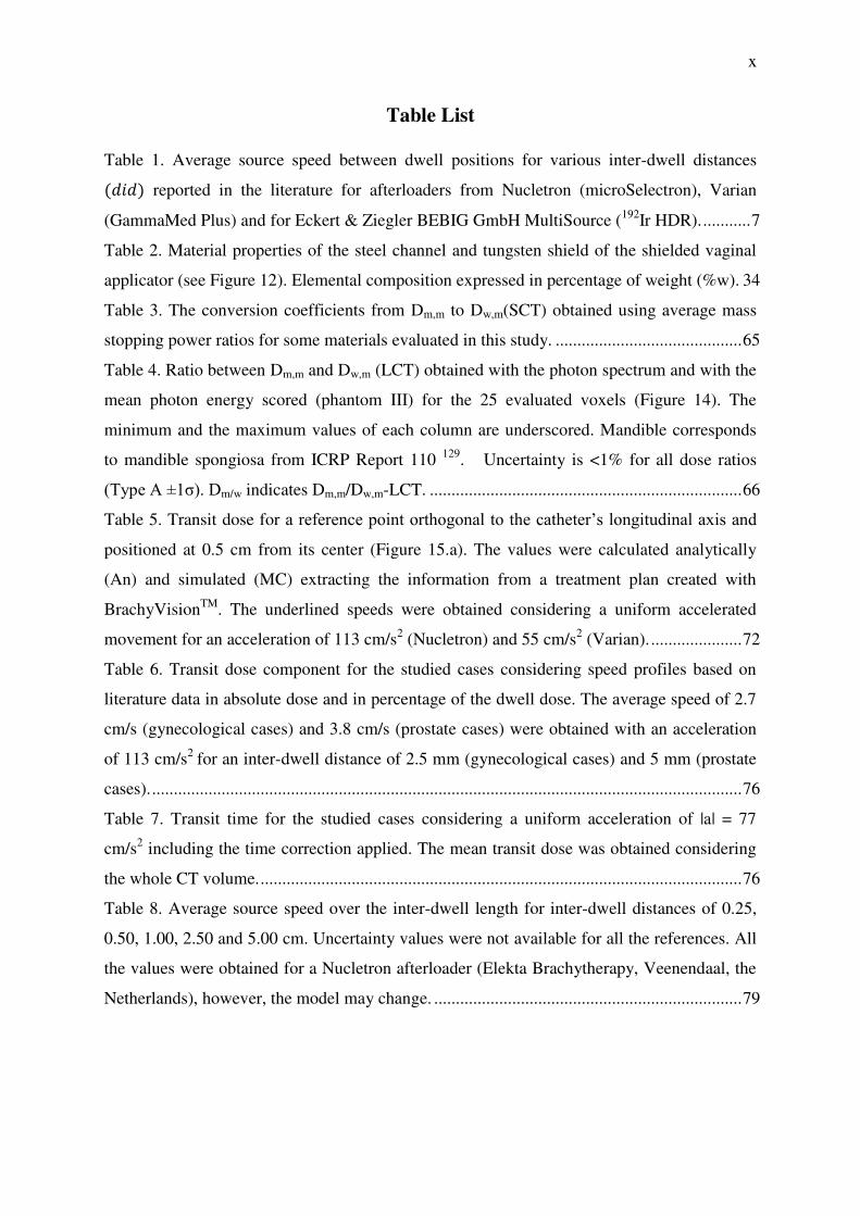
Figure 38. Prostate case d (transverse plane): a) Isodoses over a CT slice with the catheters
corresponding to the boundaries of the prostate contour; b) transit dose percentage compared
against the dwell dose. c) corrected transit dose percentage compared against the dwell dose.
Figures b and c are shown using different scales. ..................................................................... 75
Figure 39. a) Source speed profile for the source arriving at the first dwell position (0 cm)
and returning to the safe. Uncertainties Type A and Type B are almost equivalent so only
Type B component is shown. b) . values were obtained for six dwell positions equally
spaced between 0 and 5 cm (vertical dotted lines). c) . values were obtained for the source
movement between two dwell positions, at 0 cm and 5 cm. Figures b and c use the same
notation with Type A and Type B uncertainty components indicated. The source speeds at the
dwell positions were not considered, therefore figures do not show speed values equal to
zero. ........................................................................................................................................... 80
Figure 40. Transit dose components (top) for a case with six dwell positions equally spaced
between 0 and 5 cm (a) and for a case with two dwell positions (b), at 0 cm and 5 cm. The
dose reduction (dwell dose correction) applied to compensate the transit dose and the
corrected dose are shown for both cases (bottom). Dwell positons are indicated with vertical
dotted lines. ............................................................................................................................... 81
x
Table List
Table 1. Average source speed between dwell positions for various inter-dwell distances � reported in the literature for afterloaders from Nucletron (microSelectron), Varian
(GammaMed Plus) and for Eckert & Ziegler BEBIG GmbH MultiSource (192
Ir HDR). ........... 7
Table 2. Material properties of the steel channel and tungsten shield of the shielded vaginal
applicator (see Figure 12). Elemental composition expressed in percentage of weight (%w). 34
Table 3. The conversion coefficients from Dm,m to Dw,m(SCT) obtained using average mass
stopping power ratios for some materials evaluated in this study. ........................................... 65
Table 4. Ratio between Dm,m and Dw,m (LCT) obtained with the photon spectrum and with the
mean photon energy scored (phantom III) for the 25 evaluated voxels (Figure 14). The
minimum and the maximum values of each column are underscored. Mandible corresponds
to mandible spongiosa from ICRP Report 110 129
. Uncertainty is <1% for all dose ratios
(Type A ±1σ). Dm/w indicates Dm,m/Dw,m-LCT. ........................................................................ 66
Table 5. Transit dose for a reference point orthogonal to the catheter’s longitudinal axis and
positioned at 0.5 cm from its center (Figure 15.a). The values were calculated analytically
(An) and simulated (MC) extracting the information from a treatment plan created with
BrachyVisionTM
. The underlined speeds were obtained considering a uniform accelerated
movement for an acceleration of 113 cm/s2 (Nucletron) and 55 cm/s
2 (Varian). ..................... 72
Table 6. Transit dose component for the studied cases considering speed profiles based on
literature data in absolute dose and in percentage of the dwell dose. The average speed of 2.7
cm/s (gynecological cases) and 3.8 cm/s (prostate cases) were obtained with an acceleration
of 113 cm/s2
for an inter-dwell distance of 2.5 mm (gynecological cases) and 5 mm (prostate
cases). ........................................................................................................................................ 76
Table 7. Transit time for the studied cases considering a uniform acceleration of |a| = 77
cm/s2 including the time correction applied. The mean transit dose was obtained considering
the whole CT volume. ............................................................................................................... 76
Table 8. Average source speed over the inter-dwell length for inter-dwell distances of 0.25,
0.50, 1.00, 2.50 and 5.00 cm. Uncertainty values were not available for all the references. All
the values were obtained for a Nucletron afterloader (Elekta Brachytherapy, Veenendaal, the
Netherlands), however, the model may change. ....................................................................... 79
xi
LIST OF ABREVIATIONS
ACE Advanced Calculation Engine
AMIGOBrachy A Medical Image-based Graphical platfOrm - Brachytherapy module
APBI Accelerated Partial Breast Irradiation
AAPM American Association of Physicists in Medicine
CAD Computer-Aided Design
CSG Constructive Solid Geometry
CT Computed Tomography
CPE Charged Particle Equilibrium
Dw,w Dose to water in water
Dm,m Dose to medium in medium
Dw,m Dose to water in medium
Dn,m Dose to a cell nuclei in medium
DE/DF Dose Energy/Dose Function MCNP cards used to define mass-energy
absorption coefficients
EBRT External Beam Radiotherapy
EBS Electronic Brachytherapy Source
EGS Electron Gamma Shower
F4/F6 MCNP cards to define a track length tally
GATE Geant4 Application for Tomographic Emission
GEANT GEometry ANd Tracking
HDR High dose rate
LBTE Linear Boltzmann Transport Equation
LCT Large Cavity Theory
LDR Low Dose Rate
xii
MBDCA Model-Based Dose Calculation Algorithms
MC Monte Carlo
MCNP Monte Carlo N-Particle
MG Mesh Geometry
MOSFET Metal Oxide Semiconductor Field Effect Transistor
MRI Magnetic Resonance Imaging
PENELOPE Penetration and ENErgy LOss of Positrons and Electrons
QA Quality Assurance
SCT Small cavity theory
SPDTL MCNP card to use lattice speed tally enhancement
TG Task Group
TLD Thermoluminescent Dosimeter
TPS Treatment Planning System
TRUS TransRectal UltraSound

INTRODUCTION Chapter 1
INTRODUCTION | 2
1 INTRODUCTION
Brachytherapy treatments are commonly performed using the American Association
of Physicists in Medicine (AAPM) Task Group report TG-43U11, 2
absorbed dose to water
formalism, which neglects human tissue densities, material compositions, body interfaces,
body shape and dose perturbations from applicators. These effects can be significant3, 4
in the
brachytherapy photon energy range and can be included in modern treatment planning
systems (TPS) for brachytherapy by using model-based dose calculation algorithms
(MBDCA). This new approach is needed to replace the TG-43U1 absorbed dose to water
formalism with a more accurate dose estimation procedure.
The AAPM Task Group report TG-1865 recently issued guidelines towards
implementing TPS, which can take the above mentioned complexities into account. The
report recommends performing model based dose calculations such as the ones based on
Monte Carlo (MC) simulations,6-8
finite element modelling9-11
or collapsed cone
convolution.12-15
This departure from the water kernel based dose calculation approach entails
adequate modelling of applicators employed in source delivery for brachytherapy for both
low energy (<50 keV) and high energy (>50 keV) photon sources.
TG-186 describes several areas where relevant scientific efforts are necessary to move
towards MBDCA. This thesis comprehends some of these subjects and other issues relevant
for brachytherapy. 192
Ir High Dose Rate (HDR) treatments are the most relevant, but not
exclusive, subject of this study, which comprehends five main approaches: a) development of
a MBDCA algorithm as an auxiliary software to process treatment planning data,
AMIGOBrachy (A Medical Image-based Graphical platfOrm - Brachytherapy module);6 b)
the use of high fidelity CAD (Computer Aided Design)-Mesh geometry to improve
brachytherapy applicators modeling;16
c) study of different dose report quantities;5 d)
evaluation of the transit dose component for gynecological and prostate clinical cases using
speed profiles from the literature;17
e) measurement of the source speed using a high speed
camera since potentially relevant transit dose components were obtained using speed profiles
from literature.
The subjects mentioned above are part of an effort to improve brachytherapy
treatment planning accuracy following TG-186 guidelines and going beyond it since CAD-
Mesh geometry and transit dose components were not discussed in TG-186. A brief
introduction on each subject was written separately in the following items for clarity.
INTRODUCTION | 3
1.1 AMIGOBrachy
Several MBDCA software packages have been developed; two commercial TPS,
ACUROSTM
(Transpire Inc., Gig Harbor, WA)10, 11, 18
and the Advanced Calculation Engine
(ACE) (Nucletron – an Elekta Company, Veenendaal, the Netherlands),12, 14, 15, 19
and several
in-house MC based algorithms.6, 20, 21
Some MBDCA employ MC simulation codes, which
offer a high accuracy for dose calculations. However, most MC codes lack a user-friendly
interface to process the input and output data of brachytherapy dose calculations. This may
involve several medical images, imaging artifact corrections, up to hundreds of dwell
positions, and source and applicator geometries.
AMIGOBrachy6 is a software module developed using MATLAB version 8.0
(Mathworks Inc., Natick, MA) to create an efficient and powerful user-friendly graphical
interface, needed to integrate clinical treatment plans with MC simulations. It does this by
providing the main resources required to process and edit images, import and edit treatment
plans, set MC simulation parameters, run MC simulations and analyze the results. In the
current implementation, the MCNP6 (Monte Carlo N-Particle version 6)22
MC code is used
for the simulations. AMIGOBrachy’s design, main functionalities and the validation process
were described including two clinical cases; one intracavitary gynecological case and one
interstitial arm sarcoma case, both treated with an 192
Ir source.
1.2 CAD-Mesh
The modelling of complex brachytherapy applicators can be suboptimal when using a
voxel based geometry due to the sub-voxel dimensions of specific components. This may
lead to volume averaging of the details of the geometry in coarse voxels, and may therefore
lead to dose calculation errors propagating in the whole geometry. The combination of a
voxelized Cartesian grid (representing the Computed Tomography (CT) derived patient
geometry) and constructive solid geometry (CSG) describing the applicator allows applicator
modelling. However, applicator modelling using CSG can be tedious, may not allow
complete fidelity or may be highly impractical, as in the case of deformable balloon
applicators employed in accelerated partial breast irradiation (APBI).
The use of tessellated surfaces, defined by a collection of 2D tiles (e.g. triangular) of
varying dimensions, or tessellated volumes defined by a collection of varying 3D elements
(polyhedrons) can be used to describe complex geometrical shapes and offers an alternative
to CSG modelling. This is especially attractive when manufacturer CAD designs are

INTRODUCTION | 4
available. This methodology has been employed by commercial deterministic particle
transport software capable of handling mesh geometries (MG).9, 11
Recent versions of general
purpose MC codes have the ability to simulate radiation transport in tessellated or MG, thus
potentially facilitating the modelling of complex brachytherapy applicators.
MG modelling was evaluated by comparison to CSG modelling of a selection of
brachytherapy applicators: the Fletcher Williamson gynecological 192
Ir HDR brachytherapy
applicator, successfully modelled using CSG techniques by several groups,18, 23-27
a shielded
vaginal HDR applicator and an accelerated partial breast irradiation (APBI) balloon
applicator used with a 50 kV electronic brachytherapy source (EBS). Dose distributions were
obtained using the Geant428
and MCNP629
general purpose MC codes.
1.3 Dose specification
TG1865 provides guidelines to take patient and applicator non-water materials into
account and also describes the different dose reporting quantities possible; dose to medium in
medium (Dm,m), and dose to water in medium (Dw,m). Differences between dose reporting in
terms of Dm,m and Dw,m have been discussed in the literature 5, 30, 31
with arguments in favor
and against both quantities.
The way to define Dw,m depends on assumptions in the employed cavity theory
regarding the cavity dimensions compared to the ranges of secondary electrons. Absorbed
dose can be calculated to a small water cavity of cellular dimensions or to a large water
cavity of dimensions similar to the CT defined voxels used in MBDCA treatment planning.
Large Cavity Theory (LCT) uses the ratio of mass-energy absorption coefficients
(water/medium), µ / � , assuming charged particle equilibrium (CPE) for the cavity of
interest 32, 33
. Small Cavity Theory (SCT) uses the ratio between mass stopping power
(water/medium), /� � , for Bragg-Gray cavities with dimensions much smaller than the
secondary electron ranges.5, 34
In external beam radiotherapy (EBRT), where ranges of secondary electrons are
substantially longer than in brachytherapy, the cavity has been assumed to be small and
conversion between Dm,m and Dw,m is made through ratios of unrestricted mass collision
stopping power, water to medium 30, 31, 35
. To define a cavity as small, large or even
intermediate sized becomes complex in brachytherapy as ranges of secondary electrons from
low energy photons (< 50 keV) are comparable to the cellular dimensions (few µm).5
INTRODUCTION | 5
Carlsson Tedgren and Alm Carlsson evaluated, using the Burlin theory, when cavity
dimensions ranging from 1 nm to 10 mm could be assumed large, small or intermediate at
various photon energies of relevance to brachytherapy. Assumed dimensions water cavity
could be of interest to evaluate the correlation between dose reporting quantities and
biological effects.34, 36
Lindborg et al. recently found the clinical radiobiological effect (RBE)
for radiotherapy modalities ranging from kV x-rays to protons and heavier ions to correlate
with the microdosimetric quantity mean linear energy when the latter was evaluated in
volumes of nm dimensions.37
The reporting dose quantities for a cell nucleus (Dn,m) of µm
dimension, Dw,m and Dm,m were evaluated by Enger et al. for different cell nucleus
compositions.38
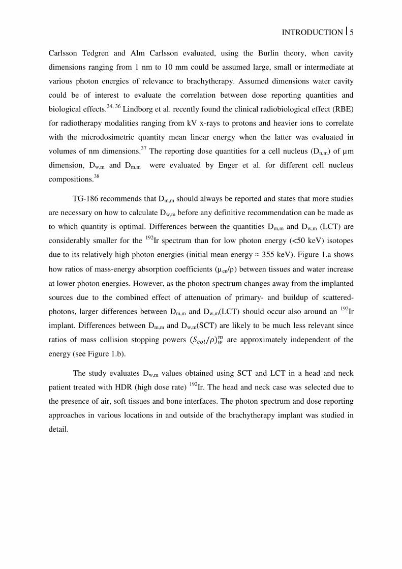
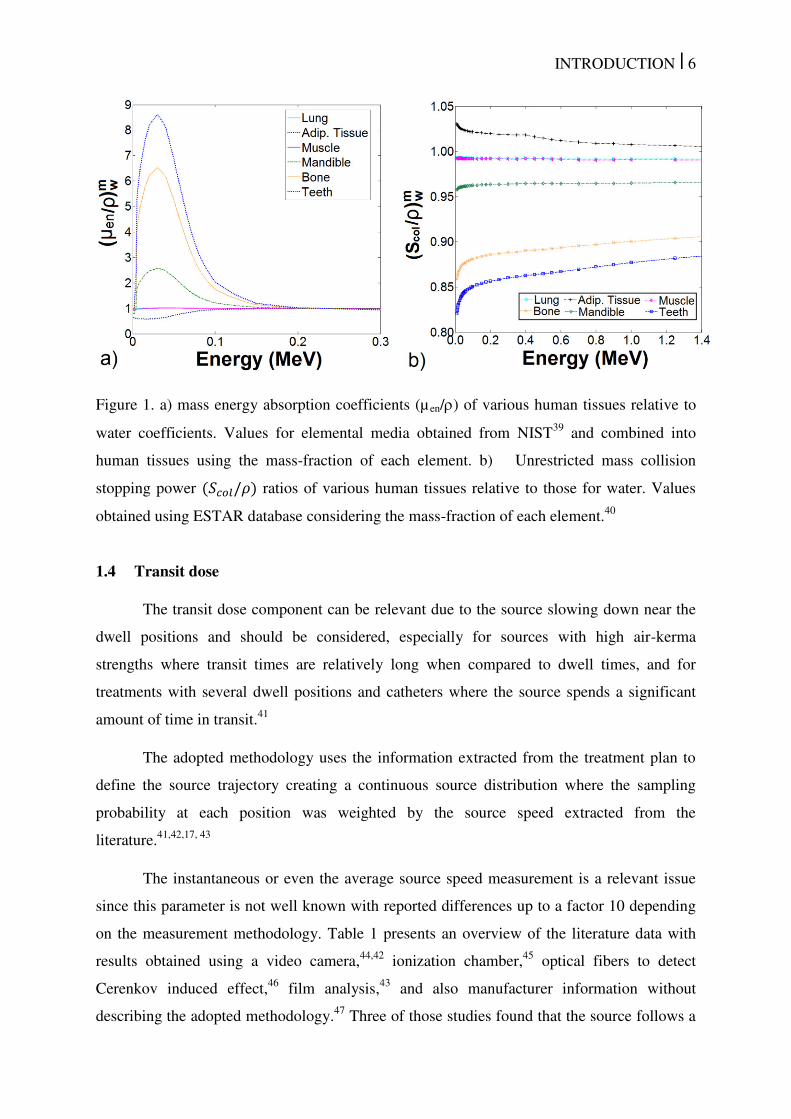
TG-186 recommends that Dm,m should always be reported and states that more studies
are necessary on how to calculate Dw,m before any definitive recommendation can be made as
to which quantity is optimal. Differences between the quantities Dm,m and Dw,m (LCT) are
considerably smaller for the 192
Ir spectrum than for low photon energy (<50 keV) isotopes
due to its relatively high photon energies (initial mean energy ≈ 355 keV). Figure 1.a shows
how ratios of mass-energy absorption coefficients (µen/) between tissues and water increase
at lower photon energies. However, as the photon spectrum changes away from the implanted
sources due to the combined effect of attenuation of primary- and buildup of scattered-
photons, larger differences between Dm,m and Dw,m(LCT) should occur also around an 192
Ir
implant. Differences between Dm,m and Dw,m(SCT) are likely to be much less relevant since
ratios of mass collision stopping powers /� � are approximately independent of the
energy (see Figure 1.b).
The study evaluates Dw,m values obtained using SCT and LCT in a head and neck
patient treated with HDR (high dose rate) 192
Ir. The head and neck case was selected due to
the presence of air, soft tissues and bone interfaces. The photon spectrum and dose reporting
approaches in various locations in and outside of the brachytherapy implant was studied in
detail.
INTRODUCTION | 6
Figure 1. a) mass energy absorption coefficients (µ en/) of various human tissues relative to
water coefficients. Values for elemental media obtained from NIST39
and combined into
human tissues using the mass-fraction of each element. b) Unrestricted mass collision
stopping power /� ratios of various human tissues relative to those for water. Values
obtained using ESTAR database considering the mass-fraction of each element.40
1.4 Transit dose
The transit dose component can be relevant due to the source slowing down near the
dwell positions and should be considered, especially for sources with high air-kerma
strengths where transit times are relatively long when compared to dwell times, and for
treatments with several dwell positions and catheters where the source spends a significant
amount of time in transit.41
The adopted methodology uses the information extracted from the treatment plan to
define the source trajectory creating a continuous source distribution where the sampling
probability at each position was weighted by the source speed extracted from the
literature.41,42,17, 43
The instantaneous or even the average source speed measurement is a relevant issue
since this parameter is not well known with reported differences up to a factor 10 depending
on the measurement methodology. Table 1 presents an overview of the literature data with
results obtained using a video camera,44,42
ionization chamber,45
optical fibers to detect
Cerenkov induced effect,46
film analysis,43
and also manufacturer information without
describing the adopted methodology.47
Three of those studies found that the source follows a
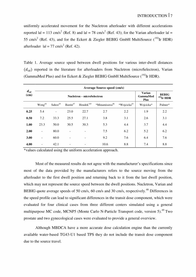
INTRODUCTION | 7
uniformly accelerated movement for the Nucletron afterloader with different accelerations
reported |a| = 113 cm/s2 (Ref. 8) and |a| = 78 cm/s
2 (Ref. 43); for the Varian afterloader |a| =
55 cm/s2 (Ref. 43), and for the Eckert & Ziegler BEBIG GmbH MultiSource (
192Ir HDR)
afterloader |a| = 77 cm/s2 (Ref. 42).
Table 1. Average source speed between dwell positions for various inter-dwell distances � reported in the literature for afterloaders from Nucletron (microSelectron), Varian
(GammaMed Plus) and for Eckert & Ziegler BEBIG GmbH MultiSource (192
Ir HDR).
��� (cm)
Average Source speed (cm/s)
Nucletron – microSelectron Varian
GammaMed Plus
BEBIG 192Ir HDR
Wong44 Sahoo45 Bastin47 Houdek145 *Minamisawa46 *Wojcicka43 Wojcicka* Palmer*
0.25 5.4 - 23.0 22.7 2.7 2.2 1.9 2.2
0.50 7.2 33.3 25.5 27.1 3.8 3.1 2.6 3.1
1.00 23.3 50.0 30.5 30.3 5.3 4.4 3.7 4.4
2.00 - 80.0 - - 7.5 6.2 5.2 6.2
3.00 - 60.0 - - 9.2 7.6 6.4 7.6
4.00 - 42.1 - - 10.6 8.8 7.4 8.8
*values calculated using the uniform acceleration approach.
Most of the measured results do not agree with the manufacturer’s specifications since
most of the data provided by the manufacturers refers to the source moving from the
afterloader to the first dwell position and returning back to it from the last dwell position,
which may not represent the source speed between the dwell positions. Nucletron, Varian and
BEBIG quote average speeds of 50 cm/s, 60 cm/s and 30 cm/s, respectively.48
Differences in
the speed profile can lead to significant differences in the transit dose component, which were
evaluated for four clinical cases from three different centers simulated using a general
multipurpose MC code, MCNP5 (Monte Carlo N-Particle Transport code, version 5).49
Two
prostate and two gynecological cases were evaluated to provide a general overview.
Although MBDCA have a more accurate dose calculation engine than the currently
available water-based TG43-U1 based TPS they do not include the transit dose component
due to the source travel.

INTRODUCTION | 8
1.5 Speed Measurements
As mentioned above the transit dose component of a brachytherapy source has been
studied previously,41-47
reporting differences up to a factor of 10 for the source speed for the
same afterloader.50
These results indicate the importance of performing more accurate source
speed profile measurements. In this work speed profiles were obtained using a high speed
video camera capable of record up to 960 fps.51
Transit dose distributions and dose reductions
due to dwell time corrections applied by the afterloader were calculated using MCNP6.22

OBJECTIVES Chapter 2

OBJECTIVES | 10
2 OBJECTIVES
The main objective of this study is to improve the accuracy of brachytherapy
treatment planning and contribute to the development of this field. It was divided in specific
objectives according to the five main subjects mentioned above:
To create an auxiliary software to process treatments plans and perform MC
simulations;
To evaluate a high fidelity CAD-mesh feature for brachytherapy applicators
modelling;
To study dose report quantities, Dw,m and Dm,m, for brachytherapy treatments;
To take into account the transit dose component due to the source movement inside
the patient using source speed profiles from the literature;
To perform accurate source speed measurements.

LITERATURE REVIEW
Chapter 3
LITERATURE REVIEW | 12
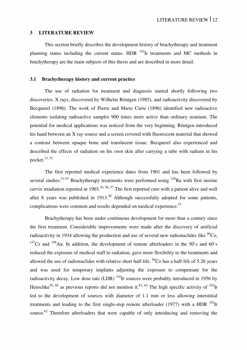
3 LITERATURE REVIEW
This section briefly describes the development history of brachytherapy and treatment
planning status including the current status. HDR 192
Ir treatments and MC methods in
brachytherapy are the main subjects of this thesis and are described in more detail.
3.1 Brachytherapy history and current practice
The use of radiation for treatment and diagnosis started shortly following two
discoveries. X rays, discovered by Wilhelm Röntgen (1985), and radioactivity discovered by
Becquerel (1896). The work of Pierre and Marie Curie (1896) identified new radioactive
elements isolating radioactive samples 900 times more active than ordinary uranium. The
potential for medical applications was noticed from the very beginning. Röntgen introduced
his hand between an X ray source and a screen covered with fluorescent material that showed
a contrast between opaque bone and translucent tissue. Becquerel also experienced and
described the effects of radiation on his own skin after carrying a tube with radium in his
pocket.13, 52
The first reported medical experience dates from 1901 and has been followed by
several studies.53-55
Brachytherapy treatments were performed using 226
Ra with first uterine
cervix irradiation reported in 1903.54, 56, 57
The first reported cure with a patient alive and well
after 8 years was published in 1913.58
Although successfully adopted for some patients,
complications were common and results depended on medical experience.57
Brachytherapy has been under continuous development for more than a century since
the first treatment. Considerable improvements were made after the discovery of artificial
radioactivity in 1934 allowing the production and use of several new radionuclides like 60
Co,
137Cs and
198Au. In addition, the development of remote afterloaders in the 50`s and 60`s
reduced the exposure of medical staff to radiation, gave more flexibility to the treatments and
allowed the use of radionuclides with relative short half-life. 60
Co has a half-life of 5.26 years
and was used for temporary implants adjusting the exposure to compensate for the
radioactivity decay. Low dose rate (LDR) 192
Ir sources were probably introduced in 1956 by
Henschke59, 60
as previous reports did not mention it.61, 62
The high specific activity of 192
Ir
led to the development of sources with diameter of 1.1 mm or less allowing interstitial
treatments and leading to the first single-step remote afterloader (1977) with a HDR 192
Ir
source.62
Therefore afterloaders that were capable of only introducing and removing the
LITERATURE REVIEW | 13
source incorporated the capability of control dwell positions and dwell times allowing patient
specific dose optimization, which still is a relevant scientific topic today.63-65
Technical and scientific improvements reduced the treatment cost, time (for HDR
treatments) and protected medical staff from radiation exposure. These reasons contributed
to more positive outcome and have led to a continuously increasing number of
brachytherapy treatments including cervix, lung, prostate, head and neck and other types of
cancer.66
Most of the HDR treatments nowadays are performed using 192
Ir sources,
although new 69
Yb and 60
Co are commercially available.
67, 68 Two modern HDR
192Ir
afterloaders are shown in Figure 2.
Figure 2. Remote afterloaders from two manufacturers: Left – microSelectron HDR
(Nucletron, an Elekta company, Stockholm, Sweden); Right – GammaMed Plus iX (Varian
Medical Systems, Inc., Palo Alto, CA).
LITERATURE REVIEW | 14
3.1.1 Treatment planning and dosimetry
Several methods have been developed to calculate treatment doses. Intracavitary
gynecological treatments used radium equivalent dosimetry (mg.Ra.h) as standard for
decades.13, 57
Interstitial treatments were performed using few methods; Patterson–Parker
dosimetry system (Manchester) defined a uniform dose, within ± 10% of the prescribed dose,
over the tumor obtained with higher concentration of source strength in the periphery.69, 70
The Quimby system used a uniform distribution of source strength obtaining a non-uniform
dose distribution.69-71
The Paris system was developed for single and double plane implants
for which sources must be linear, implants should be parallel, source centers within the same
plane and other geometric requirements.70
Application time and treatment data were obtained
from tables calculated for standard implants, which could differ from actual patient
implants.13
Dose calculation formalisms from 226
Ra equivalent dosimetry, point source
approximations, Sieverts integration and the current formalism were summarized by Rivard
et al.13
and described in detail elsewhere.1, 2, 72, 73
For brevity, only the current approach
defined by the APPM TG-43U1 is described here.1, 2
TG-431 was released in 1995 and its update
2 in 2004; this formalism is used by
commercial TPSs to calculate dose distributions through the superposition of a single dose
distribution obtained for one source. The TG-43U1 dose to water formalism requires point
sources or sources with cylindrical symmetry. Therefore, dose rate can be obtained � with
the general (2D) formalism:
� = . �. �� �,��� �0,�0 . � . �, � 1
The polar coordinate system (� and �) was adopted along the source longitudinal axis
with the origin of the coordinate system at the center of the active core. is the air kerma
strength ( m.Gy.m2.h
-1 (U)
) of each source defined as the air kerma rate multiplied by the
square of the distance.74
The dose ratio constant, �, is defined as the ratio between dose rate
at the reference point ( � , � ; � = 1 cm and � = 90°) and . The geometry function, �, � , corrects the square-law based on approximate models of the source active core
(point and linear sources). The radial function, � , accounts for dose fall-off on the
transverse-plane due to photon scattering and attenuation. The anisotropy function, �, � ,
describes the variation in dose as a function of polar angle relative to the transverse plane.
LITERATURE REVIEW | 15
TG-43U1 parameters have been extensively described in the literature for several
brachytherapy sources.75-77
The simplistic approach and tabulated parameters allow short
calculation times leading to a successful clinical implementation. Although largely employed,
the dose to water formalism fails to consider the body dimensions, lack of backscattering,
applicator effects and inter-seed attenuation.5, 13
3.1.1.1 TG-43U1 limitations and TG-186
Some of TG-43U1 limitations are well known, however the scientific and technical
challenges to move towards approaches that are more accurate, as MBDCA, are significant.
TG-186 describes some of TG-43U1 limitations, the status of scientific development and
areas where efforts are necessary. The recent protocol was released during a period when a
commercial MBDCA was available, ACUROSTM
.10, 11, 18
Currently, Advanced Calculation
Engine (ACE) (Nucletron – an Elekta Company, Veenendaal, the Netherlands),12, 14, 15, 19, 78
is
also available. Therefore, issues such as tissue segmentation, CT scanner calibration, dose
report quantities, applicator models and other issues related to MBDCA, which can affect
brachytherapy treatments, became relevant for the medical staff and can affect brachytherapy
treatments.
A discussion about some of TG-186 main subjects is included below. Dose report
quantities (Dw,m and Dm,m), widely described in TG-186, are discussed in section 1.3 (Dose
specification) as it is one of the main topics of this thesis. Transit dose component (section
1.4 - Transit dose) and mesh geometries (section 1.2 - CAD-Mesh) are discussed in a
different section for the same reason.
3.1.1.1.1 Medical images and segmentation
Brachytherapy treatments involved palpation or visualization of the structures with
implant reconstruction obtained using orthogonal x rays, which did not allow anatomy based
treatment planning. Therefore, treatments were performed using the applicator as reference
and not the patient.13, 66, 79
3D image guided implants and post implant dose calculation
started with pioneering studies during 80’s and 90’s. The first reported use of a transrectal
ultrasound (TRUS) dates from 1983 followed by several studies that consolidated this
methodology.79-82
Nowadays, TRUS, CT and magnetic resonance imaging (MRI) are
commonly used for real time imaging (TRUS) and treatment planning. Medical images
obtained with TRUS, CT and MRI and a 3D reconstruction are shown in Figure 3.
LITERATURE REVIEW | 16
Figure 3. a) TRUS image of a prostate patient; b) CT image of a head and neck patient; c)
MRI image of a gynecological patient; d) 3D reconstruction from CT images including the
clinical target volume (CTV) in red.
CT images provide information about the atomic number and mass (or electronic)
density, which can be employed for tissue segmentation.83
Dual energy CT scanners that
acquire images using two different x-ray energy spectra may allow a more accurate extraction
of tissue characteristics.84-86
These characteristics are highly important for low energy
brachytherapy sources for which photoelectric effect is dominant. Therefore, energy deposition
is highly dependent on tissue composition as can be seen by the mass absorption coefficients
(µen/) of various human tissues relative to water (Figure 1).3, 8, 33
Other modalities such as MRI
and US do not provide electronic densities, but may provide excellent visualization of soft
tissue (MRI - Figure 3.c) and real time visualization to outline organs as prostate and urethra
(US - Figure 3.a). All imaging techniques are greatly aided by image registration between
LITERATURE REVIEW | 17
either CT and MRI or CT and US for which CT based speed of sound correction, due to
different tissues densities, are being evaluated to improve US images.87
Although highly relevant for low energy sources, tissue segmentation may not be
necessary for 192
Ir energies. Rivard et al.13
discussed which commonly treated anatomic sites
(prostate, breast, gynecological, skin, lung, penis and eye) may show significant differences
between the actual calculation formalism (TG43-U1 homogeneous water phantom) and more
accurate models (MBDCA). None of the evaluated sites are expected to show significant
differences, for 192
Ir photon spectrum, due to tissue composition or attenuation. Differences
are expected only due to shielding (gynecological, skin and eye) or scattering (breast, skin,
lung penis and eye) due to interfaces with air.13
Therefore, a homogeneous phantom with
image-defined boundaries may provide accurate dose calculations for high-energy
brachytherapy sources.
Proper tissue segmentation may not be possible even using CT images since image
artifacts may not allow it as shown in Figure 4. Image artifacts that degrade image quality are
due to the image reconstruction algorithm88
processing transit images with high atomic
number and density and may lead to wrong tissue and density assignment. Several methods
have been employed to correct image artifacts, from manual contouring to sophisticated
interactive algorithms, filtered images and sinograms.88-91
Currently, efficient and robust
methods are not commonly available and the potential of these algorithms to improve dose
calculation accuracy needs to be studied (see section 4.4 Dose specification (Dw,m and Dm,m)
for more information about material misassignment).5
Figure 4. CT slices of a head and neck patient showing metal artifacts.
LITERATURE REVIEW | 18
3.1.2 Brachytherapy applicators and shielding effects
Brachytherapy treatments may employ plastic or metal needles92
and a wide variety of
applicators, from single channel cylinders to more complex applicators with several channels
and shielding.10, 16, 26, 93
Moreover, some applicators such as balloons used for APBI may
assume patient cavity shapes as discussed in section 4.3 (CAD-Mesh) and evaluated by
White et al.8 for clinical cases.
Petrokokkinos et al. evaluated a shielded cylinder applicator (GM11004380 – a
similar model was represented in section 4.3.1.4 - Shielded HDR vaginal applicator) with
measurements and simulations using three dose calculation engines: ACUROSTM
, a MC
code and a commercial TPS (TG-43U1). Results showed differences of up to 90% between
MC and TG-43U1 in the shielded side and up to 10% for clinically relevant points close to
the applicator in the unshielded side as scatter reduction due to the partial shield was not
taken into account by the TPS (TG-43U1).10
Results obtained using ACUROSTM
and MC are
almost equivalent except for differences between 2% and 10% in the penumbra of the
shield.10
The Fletcher Williamson shielded applicator for HDR 192
Ir sources was extensively
studied by several groups.18, 23-27
A MG model of this applicator was evaluated in this thesis
and described in section 4.3.1.5 (Shielded HDR Fletcher Williamson applicator). This
applicator was developed to reduce doses in organs at risk (bladder and rectum). A ratio
between dose distributions obtained using a MC with and without the applicator is shown in
Figure 5 for illustrative purposes. Results with and without the applicator are almost
equivalent in the unshielded region (near the tip) though significant differences are visible in
other regions. Applicator effects are considerable and may allow dose escalation as heathy
structures can be preserved.
Dosimetric perturbations of a lead shield was studied by Candela-Juan et al. for 60
Co,
192Ir and
169Yb sources used for surface and interstitial HDR brachytherapy. An overdose near
the shield, mainly due to backscattered electrons, can reach a factor of 3 at 0.1 mm from the
shield for a 192
Ir source. Tissues can be preserved by adding 3 mm and 1 mm of bolus around
the shield for 60
Co and 192
Ir, respectively.
Although shielded applicators show the most significant differences from TG-43U1
dose to water formalism, differences up to 5% within the target volume were observed for a
gynecological case due to a hollow applicator (see sections 4.2.4.1 and 5.1.2).6
LITERATURE REVIEW | 19
Figure 5. Ratio between dose distributions obtained with MC with and without including the
Fletcher Williamson applicator. The dark blue region represents the applicator.
3.2 MC methods in brachytherapy
MC method is widely employed in several fields as astronomy, meteorology, traffic
prediction and medical physics. In medical physics MC has been employed to simulate linear
accelerators,94
patients,95
brachytherapy sources,76
energy dependence of dosimeters,96
neutron stimulated emission computed tomography,97
to calculate ion chamber correction
factors due to wall attenuation and scatter98-100
, and for several other applications. Rogers
published a review about MC simulations for medical physics.101
He searched for the term
‘Monte Carlo’ on PubMed† getting 14452 hits as of January 2006 whilst the same search
performed 9 years later (January 2015) showed 38901 hits. The number of papers per year
including the term ‘Monte Carlo’ is shown in Figure 6. The increase use of MC codes is
related to the increase in computing power that allows shorter simulation times.
Several MC codes are available comprising a wide variety of applications. MCNP was
originally developed to transport neutrons and photons. Currently, MCNP can transport
several particles as photons, neutrons, electrons, protons, heavy ions and others.22, 49
† http://www.ncbi.nlm.nih.gov/pubmed/
LITERATURE REVIEW | 20
PENELOPE (Penetration and ENErgy Loss of Positrons and Electrons)102
transports
electrons, positrons and photons. GEANT4 (GEometry ANd Tracking) transports a wide
variety of particles and is the basis of GATE (Geant4 Application for Tomographic
Emission).28, 103
EGS (Electron Gamma Shower) is a photon-electron coupled code
considered the most used general purpose MC code in medical physics.101
Recent data about
MC codes usage were not found. However, a refined search within papers with the term
‘Monte Carlo’ shows 637 papers with at least one of the expressions ‘MCNP’, ‘MCNP4’,
‘MCNP5’ or ‘MCNP6’; 643 with at least one of the terms ‘GEANT’, ‘GEANT4’, ‘G4’ or
‘GATE’; 218 papers with the term ‘PENELOPE’; 809 papers with at least one of the terms
‘EGS’, ‘EGSnrc’, ‘EGS3’, ‘EGS4’, or ‘BrachyDose’. Results indicated that EGS, and its
versions, is still the most used code. However, other codes are almost equally used.
Figure 6. Number of papers per year including the term ‘Monte Carlo’. Results of a PubMed
search (20 January 2015).
MC plays a key role in brachytherapy for clinical practice and research. The first
computational efforts to obtain dose distributions around brachytherapy sources date from the
60’s, with 3D models used as early as 1971.7, 104, 105
Landry et al. summarized some results
obtained during the 90’s comparing MC dose distributions against experimental data using
thermoluminescent dosimeters (TLD) and diodes.7 Agreement within 5% for
125I and 3% for
192Ir sources validated MC calculations.
106-111 TG-43 recommends that at least one
experimental and one MC calculation of dosimetry parameters should be published before
using a source clinically.1, 2
This recommendation consolidated MC as a standard for
LITERATURE REVIEW | 21
brachytherapy. Moreover, experimental measurements are complex due to the sharp dose
gradient in the brachytherapy energy range. However, MC should not be trusted blindly as
pointed out by Williamson et al.108
MC code is a gold standard MBDCA whose importance goes beyond source models
as patient specific dose calculations can be performed. Despite its well-known accuracy, MC
has not been implemented in clinical practice due to its calculation time.112
Significant
computational requirements are inherent of a stochastic method for radiation transport that
must simulate a large number of particles to produce statistically relevant results. This may
no longer be a problem due to the computational power available nowadays.112
Currently, the
simulation time necessary to obtain an average dose uncertainty of 2% for an intracavitary
case with 6.6x10⁶ voxels is 27 min using an Intel Xeon X5650 processor with twelve cores of
2.67GHz and 32 Gb of RAM. This is reduced to 5 min on a SGI C2112 server (Silicon
Graphics International Corporation, Chippewa Falls, USA) consisting of 16 processors with
eight cores of 2.4 GHz each.6 Landry et al. obtained calculation time about 6 and 12 min for
2% uncertainty for a breast and a prostate implant, respectively.7 Literature reported MC
results obtained within seconds for low-energy sources and few minutes for 192
Ir.112
Such
simulation times may be suitable for a future clinical implementation.
Other issues related to MC are described within this thesis according with the studied
subject, e.g. Track length estimators (section 4.1.1.2), dose report quantities (sections 1.3, 4.4
and 5.3), applicator modelling (sections 4.2.1 and 4.3 and 5.2).

MATERIALS AND METHODS
Chapter 4
MATERIALS AND METHODS | 23
4 MATERIALS AND METHODS
4.1 Monte Carlo codes
This section includes general information about the MC codes used in this thesis
whilst specific simulation parameters were described in each section.
4.1.1 MCNP
MCNP version 5 and 6 were used in this thesis since only version 5 was available by
the time some results were obtained. No differences were observed between the versions,
except for MCNP6 new features as CAD-Mesh. MCNP is a multipurpose radiation MC
transport code22, 113
widely employed in medical physics,8, 93
which can involve high-
resolution voxel phantoms. Therefore, MC codes must handle a large amount of data
requiring a large RAM memory and long CPU times. To increase simulation efficiency the
Harvard/MIT Boron Neutron Capture Therapy clinical trials team developed lattice speed
tally enhancement (LSTE) for simulations with large number of voxels.29
The LSTE function can be employed under specific situations such as: a) a hexagonal
lattice must be present in the geometry; b) all F4 (MCNP6 tally) tallies contain a hexahedral
lattice; c) all F4 tallies have associated DE/DF cards; d) nested lattices are scored together.
However, this function is not compatible with all tallies. Simulations with F4 tallies can be
faster by a factor of 100 or more than simulations with F6 (MCNP6 tally) tallies since LSTE
does not work for F6 tallies even though both tallies are track length based estimators. When
the SPDTL card is active, tracking is more efficient since it considers only lattice geometries
enclosed in a parallelepiped, removes general surface checks, removes extraneous energy
bins and tally modifiers. LSTE retains only the tally multipliers (DE/DF cards) necessary to
convert average photon energy fluence to kerma29
.
MCNP6 calculations were performed using a track length estimator tally, using the
MCPLIB84 photon cross-section library in Mode P which means secondary electrons were
not transported (therefore, kerma was scored), except for one simulation described in item
4.1.1.3 (Pulse height tallies). Results were converted to collision kerma using mass-energy
absorption coefficients from NIST.114
All cases were simulated using the 192
Ir photon
spectrum available from the National Nuclear Data Center (NNDC)115
. Photons were
transported down to an energy cut-off of 1 keV.
MATERIALS AND METHODS | 24
4.1.1.1 MCNP6 mesh capability
The capability of handling mesh geometries was recently included in the MCNP6 beta
2 release, which can handle first and second order tetrahedral, pentahedral and hexahedral
elements defined through text files directly generated by two commercial programs,
AbaqusTM
(Dessault Systèmes, France) and ATTILA (Transpire Inc., Gig Harbor, WA) or by
converting the volume elements generated by other programs, such as ENGRID or GMSH.
116
We opted for tetrahedral meshes defined using the .ele/.node files used for Geant4
simulations converted to the MCNP6 format.117
4.1.1.2 Track length estimator tallies
Track length estimator tallies can be used under CPE conditions, which is achieved
for the 192
Ir spectrum for distances greater than 2 mm from the source.118, 119
Under CPE
conditions dose values are approximate by collision kerma (and even kerma in low atomic
number materials where bremsstrahlung is negligible) and can be obtained by multiplying the
energy fluence (E.ФE) by µen/ as described in equation 2. Fluence values were scored for N
energy bins (i) with 1 keV resolution using MCNP6. This methodology is efficient since the
number of tracks crossing a voxel is much higher than the number of interactions in it and
leads to accurate results within the brachytherapy energy range for mm-sized voxels.8, 76, 120
This approach is followed in the first MC simulation (track length) mentioned above.
≈ ∑ [Ф�� � . �. µ��� � � ]��= 2
4.1.1.3 Pulse height tallies
Pulse height tallies are analogous estimators121
(like a physical detector) scoring the
energy deposited per interaction inside of the scoring volume. It is an accurate method, even
without CPE, with the penalty of being statistically less efficient than track length tallies.
This approach does not introduce significant uncertainties since electrons with 50 keV energy
have a mean residual range of 0.04 mm in water that is almost ten times shorter than the
smallest voxel dimension,122
and bremsstrahlung production below 50 keV in water and low
atomic number material is completely negligible.123
Only one simulation was performed
using this tally to quantify possible differences due to the absence of CPE that may occur for
MATERIALS AND METHODS | 25
small scoring volumes and near material interfaces (see section 4.4 - Dose specification (Dw,m
and Dm,m) for more information).13, 34
Dm,m values including effects of electron transport were
obtained simulating the whole CT geometry. However, dose values were scored only for one
sagittal slice to reduce the simulation time since it increases with the number of scoring
volumes, which can make simulations impractical.
4.1.2 Geant4
The MC toolkit Geant4.9.5.p02 was used in this thesis, using the
G4EmLivermorePhysics class for low energy electromagnetic physics and the layered mass
geometry method.124
The code was used to validate MCNP6 calculations with mesh
geometries (section 4.3 - CAD-Mesh). A voxel grid was used to represent the patient
geometry derived from CT imaging and a parallel world contains the model of a
brachytherapy source and applicator. In locations where voxels and applicator model
overlapped, photons were transported in the latter.
To perform MG modelling we installed the Geant4 library CADMesh version 0.6.2
(Ref. 125) which enables the import of tessellated surfaces or volumes. It has been reported126
that the use of tessellated surfaces based on the G4TessellatedSolid class requires longer
simulation times than tessellated volumes based on an assembly of G4Tet (Geant4 class for
modelling tetrahedra). This was confirmed in our work; therefore the latter approach was
used. Several file formats are supported by CADMesh; An .ele and .node description of
volume meshes composed of a collection of tetrahedrons was adopted.‡ The .node file
contains a list of vertices which are grouped in the .ele file to describe volume elements.
Volumes represented by a collection of tetrahedrons will be referred as MG. Upon import via
CADMesh in Geant4 the .ele/.node tetrahedral mesh yields a G4Assembly volume (a class
allowing to group a number of volumes such as G4Tet) to which a position in the parallel
world and a material can be assigned.126
4.2 AMIGOBrachy
AMIGOBrachy has been developed using MATLAB version 8.0 with the aim of
providing tools such as: a) medical image processing, b) dwell position identification, c)
needle detection, d) phantom creation using DICOM images, e) MCNP6 code input file
‡ http://tetgen.berlios.de/fformats.ele.html
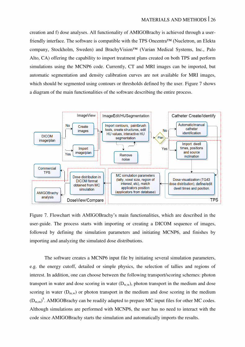
MATERIALS AND METHODS | 26
creation and f) dose analyses. All functionality of AMIGOBrachy is achieved through a user-
friendly interface. The software is compatible with the TPS Oncentra™ (Nucletron, an Elekta
company, Stockholm, Sweden) and BrachyVision™ (Varian Medical Systems, Inc., Palo
Alto, CA) offering the capability to import treatment plans created on both TPS and perform
simulations using the MCNP6 code. Currently, CT and MRI images can be imported, but
automatic segmentation and density calibration curves are not available for MRI images,
which should be segmented using contours or thresholds defined by the user. Figure 7 shows
a diagram of the main functionalities of the software describing the entire process.
Figure 7. Flowchart with AMIGOBrachy’s main functionalities, which are described in the
user-guide. The process starts with importing or creating a DICOM sequence of images,
followed by defining the simulation parameters and initiating MCNP6, and finishes by
importing and analyzing the simulated dose distributions.
The software creates a MCNP6 input file by initiating several simulation parameters,
e.g. the energy cutoff, detailed or simple physics, the selection of tallies and regions of
interest. In addition, one can choose between the following transport/scoring schemes: photon
transport in water and dose scoring in water (Dw,w), photon transport in the medium and dose
scoring in water (Dm,w) or photon transport in the medium and dose scoring in the medium
(Dm,m)5. AMIGOBrachy can be readily adapted to prepare MC input files for other MC codes.
Although simulations are performed with MCNP6, the user has no need to interact with the
code since AMIGOBrachy starts the simulation and automatically imports the results.
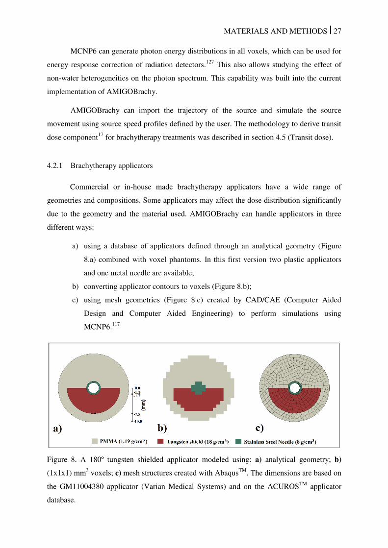
MATERIALS AND METHODS | 27
MCNP6 can generate photon energy distributions in all voxels, which can be used for
energy response correction of radiation detectors.127
This also allows studying the effect of
non-water heterogeneities on the photon spectrum. This capability was built into the current
implementation of AMIGOBrachy.
AMIGOBrachy can import the trajectory of the source and simulate the source
movement using source speed profiles defined by the user. The methodology to derive transit
dose component17
for brachytherapy treatments was described in section 4.5 (Transit dose).
4.2.1 Brachytherapy applicators
Commercial or in-house made brachytherapy applicators have a wide range of
geometries and compositions. Some applicators may affect the dose distribution significantly
due to the geometry and the material used. AMIGOBrachy can handle applicators in three
different ways:
a) using a database of applicators defined through an analytical geometry (Figure
8.a) combined with voxel phantoms. In this first version two plastic applicators
and one metal needle are available;
b) converting applicator contours to voxels (Figure 8.b);
c) using mesh geometries (Figure 8.c) created by CAD/CAE (Computer Aided
Design and Computer Aided Engineering) to perform simulations using
MCNP6.117
Figure 8. A 180º tungsten shielded applicator modeled using: a) analytical geometry; b)
(1x1x1) mm3 voxels; c) mesh structures created with Abaqus
TM. The dimensions are based on
the GM11004380 applicator (Varian Medical Systems) and on the ACUROSTM
applicator
database.
MATERIALS AND METHODS | 28
The applicator’s position can be obtained from DICOM file headers, when available,
or defined by the user through two or more points depending on the applicator geometry.
Moreover, applicators can consist of one or more small and/or thin structures, which cannot
be accurately represented by regular voxels (i.e. the hollow needle in Figure 8.b).
4.2.2 Validation
Dose distributions obtained with AMIGOBrachy/MCNP6 were compared against
dose distributions exported from BrachyVisionTM
version 10.0 employing a Linear
Boltzmann Transport Equation (LBTE) solver, ACUROSTM
, which can handle non-water
heterogeneities.10, 11, 18, 128
4.2.3 Uniform phantoms
The validation process involved several steps going from source parameter validation
up to clinical case comparisons against a commercial TPS. AMIGOBrachy currently models
two HDR 192
Ir sources; microSelectron77
(Nucletron), and GammaMed Plus76
(Varian), and
an electronic brachytherapy X-ray source (Axxent; Xoft, San Jose, CA).120
The sources were
validated by comparing TG43-U11, 2
parameters such as anisotropy function, radial function
and air kerma strength against values from the literature (data not show). Dwell times and
dwell positions were validated by comparing the MC input generated with AMIGOBrachy
against DICOM header information and reports from TPS.
Material compositions and dose grid effects were verified by comparing dose
distributions obtained with a DICOM object of 200x200x200 voxels, with a 1 mm resolution,
consisting of a cubic phantom (10x10x10 cm3) positioned in the middle of the image and
surrounded by air was created for validation purposes. Simulations were performed for 9
dwell positions within homogeneous phantoms consisting of all tissues available in the
ACUROSTM
library (lung, adipose tissue, water, muscle, cartilage and bone)129
using dose
scoring grids of 1 mm slice thickness and a width/height of 0.50, 1, 2.50 and 5.0 mm.
4.2.4 Clinical cases
Two treatment plans were created for a GammaMed Plus 192
Ir source using DICOM
patient images from one interstitial and one intracavitary case. The dose distributions were
calculated considering the material compositions and densities provided in the ACUROSTM

MATERIALS AND METHODS | 29
user guide. The dose grid resolution was the same as the image resolution used in each case,
while the dose grid sizes (i.e. the number of voxels) were defined interactively considering
the ACUROSTM
memory requirements. The distance between the isodoses and the dose
values per voxel were compared.
The treatment plans were then imported in AMIGOBrachy to generate MCNP6 input
files by reproducing the TPS configuration. This includes tissue contours, materials, dwell
positions, applicator, dose grid and voxel size. Dose calculations were reported as Dw,w (as
adopted by TG-43U1) and Dw,m, with the type A (k=1) simulation uncertainty component less
than 1% within the region covered by the 30% isodose.
A sequence of images illustrating the steps necessary to perform a simulation using a
treatment plan imported by AMIGOBrachy is shown in Figure 9.
Figure 9. A sequence of images used by AMIGOBrachy: a) importing the DICOM patient
CT image; b) defining structures by importing DICOM contours (e.g. the highlighted bone
contours); c) defining the material map (using HU numbers or drawing tools), which consists
of air (black region), adipose tissue (blue region), muscle (green region) and bone (yellow
region); d) defining the voxel phantom region (external rectangle) and the dose scoring
region (internal rectangle).
4.2.4.1 Intracavitary case
The treatment plan for an intracavitary gynecological case was made with a DICOM
CT image set consisting of 63 slices with 512x512 voxels, 3 mm slice thickness and voxel
size of 0.98 mm. Dose distributions were calculated for a single guidance needle in the
middle of a hollow plastic cylinder applicator (external diameter of 3.5 cm and 0.4 cm wall
thickness). The applicator is placed in a phantom representing the patient with all voxels
MATERIALS AND METHODS | 30
assigned to one of six materials (polyphenylsulfone (modelling the applicator), water, bone,
muscle, adipose tissue and air) from the ACUROSTM
database. There are 17 dwell positions
and the prescribed dose is 7.5 Gy per fraction at 0.5 cm from the applicator’s outer wall. The
following situations were considered: a) “infinite” homogeneous water phantom with at least
20 cm of water between the scoring voxels and the closest boundary with air130
; b) body
boundaries defined using CT images with all materials assigned as water, including the
applicator; c) CT based geometry where tissues are assigned as water and the applicator
assigned with its real composition; d) CT based geometry with tissues and applicator
assigned with their proper composition. Air was assigned to the regions outside the body
except for case a.
4.2.4.2 Interstitial case
The treatment plan for an interstitial arm sarcoma case was made with a DICOM CT
image set consisting of 253 slices with (512 x 512) voxels, 1.25 mm slice thickness and pixel
spacing of 0.59 mm. Dose distributions were calculated considering 9 channels, 106 dwell
positions and a total dwell time of 336.6 s. The following situations were considered: a)
“infinite” homogeneous water phantom, as defined in the previous validation case; b) all
tissues assigned as water; c) all tissues assigned as muscle; d) tissues assigned as muscle and
bone. Plastic catheters were not modeled and air was assigned to the regions outside the body
except for case a.
4.3 CAD-Mesh
4.3.1 Geometries of interest
Three types of applicators were considered in this thesis; two gynecological
applicators used with an 192
Ir HDR source and a balloon applicator used with an EBS
operated at 50 kVp. The 192
Ir spectrum was taken from National Nuclear Data Center 115
and
the 50 kV spectrum from Liu et al. 131
using a Geant4 model based on the work of Rivard et
al. 132
. Additionally, simpler geometries such as a water cube and a spherical APBI applicator
were employed for estimation of calculation efficiency and validation. All geometries were
simulated with both MC codes using the same MG. Although there are differences between
the input formats, both codes use the same information, which are nodes (defined using
cartesian coordinates) and faces (defined through node connections).
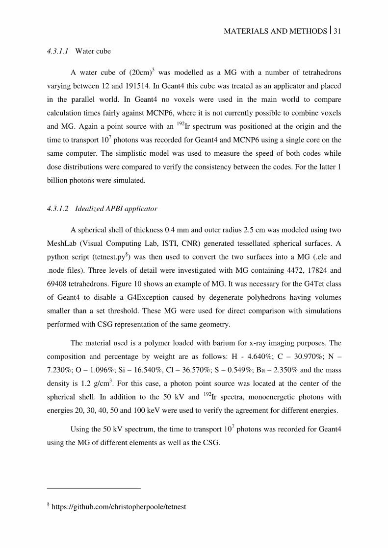
MATERIALS AND METHODS | 31
4.3.1.1 Water cube
A water cube of (20cm)3 was modelled as a MG with a number of tetrahedrons
varying between 12 and 191514. In Geant4 this cube was treated as an applicator and placed
in the parallel world. In Geant4 no voxels were used in the main world to compare
calculation times fairly against MCNP6, where it is not currently possible to combine voxels
and MG. Again a point source with an 192
Ir spectrum was positioned at the origin and the
time to transport 107 photons was recorded for Geant4 and MCNP6 using a single core on the
same computer. The simplistic model was used to measure the speed of both codes while
dose distributions were compared to verify the consistency between the codes. For the latter 1
billion photons were simulated.
4.3.1.2 Idealized APBI applicator
A spherical shell of thickness 0.4 mm and outer radius 2.5 cm was modeled using two
MeshLab (Visual Computing Lab, ISTI, CNR) generated tessellated spherical surfaces. A
python script (tetnest.py§) was then used to convert the two surfaces into a MG (.ele and
.node files). Three levels of detail were investigated with MG containing 4472, 17824 and
69408 tetrahedrons. Figure 10 shows an example of MG. It was necessary for the G4Tet class
of Geant4 to disable a G4Exception caused by degenerate polyhedrons having volumes
smaller than a set threshold. These MG were used for direct comparison with simulations
performed with CSG representation of the same geometry.
The material used is a polymer loaded with barium for x-ray imaging purposes. The
composition and percentage by weight are as follows: H - 4.640%; C – 30.970%; N –
7.230%; O – 1.096%; Si – 16.540%, Cl – 36.570%; S – 0.549%; Ba – 2.350% and the mass
density is 1.2 g/cm3. For this case, a photon point source was located at the center of the
spherical shell. In addition to the 50 kV and 192
Ir spectra, monoenergetic photons with
energies 20, 30, 40, 50 and 100 keV were used to verify the agreement for different energies.
Using the 50 kV spectrum, the time to transport 107 photons was recorded for Geant4
using the MG of different elements as well as the CSG.
§ https://github.com/christopherpoole/tetnest
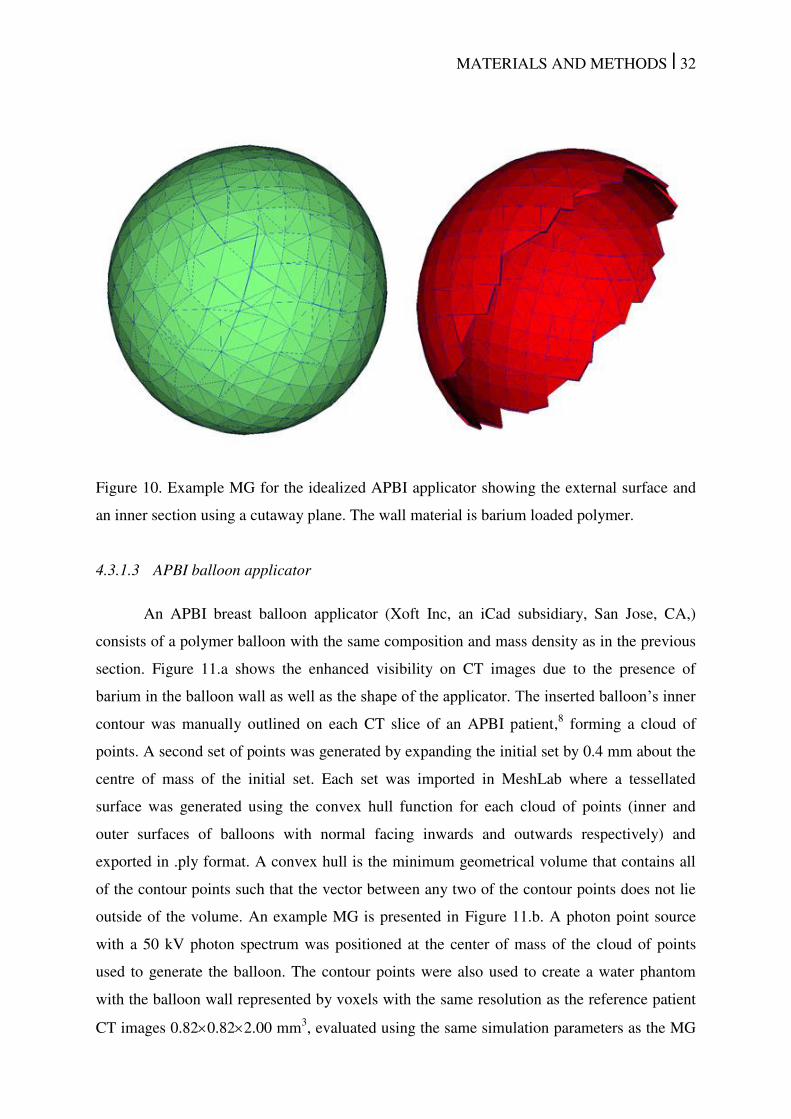
MATERIALS AND METHODS | 32
Figure 10. Example MG for the idealized APBI applicator showing the external surface and
an inner section using a cutaway plane. The wall material is barium loaded polymer.
4.3.1.3 APBI balloon applicator
An APBI breast balloon applicator (Xoft Inc, an iCad subsidiary, San Jose, CA,)
consists of a polymer balloon with the same composition and mass density as in the previous
section. Figure 11.a shows the enhanced visibility on CT images due to the presence of
barium in the balloon wall as well as the shape of the applicator. The inserted balloon’s inner
contour was manually outlined on each CT slice of an APBI patient,8 forming a cloud of
points. A second set of points was generated by expanding the initial set by 0.4 mm about the
centre of mass of the initial set. Each set was imported in MeshLab where a tessellated
surface was generated using the convex hull function for each cloud of points (inner and
outer surfaces of balloons with normal facing inwards and outwards respectively) and
exported in .ply format. A convex hull is the minimum geometrical volume that contains all
of the contour points such that the vector between any two of the contour points does not lie
outside of the volume. An example MG is presented in Figure 11.b. A photon point source
with a 50 kV photon spectrum was positioned at the center of mass of the cloud of points
used to generate the balloon. The contour points were also used to create a water phantom
with the balloon wall represented by voxels with the same resolution as the reference patient
CT images 0.820.822.00 mm3, evaluated using the same simulation parameters as the MG
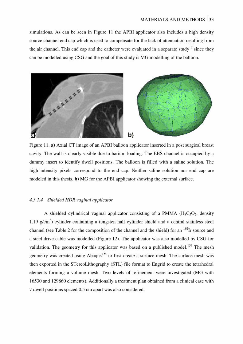
MATERIALS AND METHODS | 33
simulations. As can be seen in Figure 11 the APBI applicator also includes a high density
source channel end cap which is used to compensate for the lack of attenuation resulting from
the air channel. This end cap and the catheter were evaluated in a separate study 8 since they
can be modelled using CSG and the goal of this study is MG modelling of the balloon.
Figure 11. a) Axial CT image of an APBI balloon applicator inserted in a post surgical breast
cavity. The wall is clearly visible due to barium loading. The EBS channel is occupied by a
dummy insert to identify dwell positions. The balloon is filled with a saline solution. The
high intensity pixels correspond to the end cap. Neither saline solution nor end cap are
modeled in this thesis. b) MG for the APBI applicator showing the external surface.
4.3.1.4 Shielded HDR vaginal applicator
A shielded cylindrical vaginal applicator consisting of a PMMA (H8C5O2, density
1.19 g/cm3) cylinder containing a tungsten half cylinder shield and a central stainless steel
channel (see Table 2 for the composition of the channel and the shield) for an 192
Ir source and
a steel drive cable was modelled (Figure 12). The applicator was also modelled by CSG for
validation. The geometry for this applicator was based on a published model.133
The mesh
geometry was created using AbaqusTM
to first create a surface mesh. The surface mesh was
then exported in the STereoLithography (STL) file format to Engrid to create the tetrahedral
elements forming a volume mesh. Two levels of refinement were investigated (MG with
16530 and 129860 elements). Additionally a treatment plan obtained from a clinical case with
7 dwell positions spaced 0.5 cm apart was also considered.
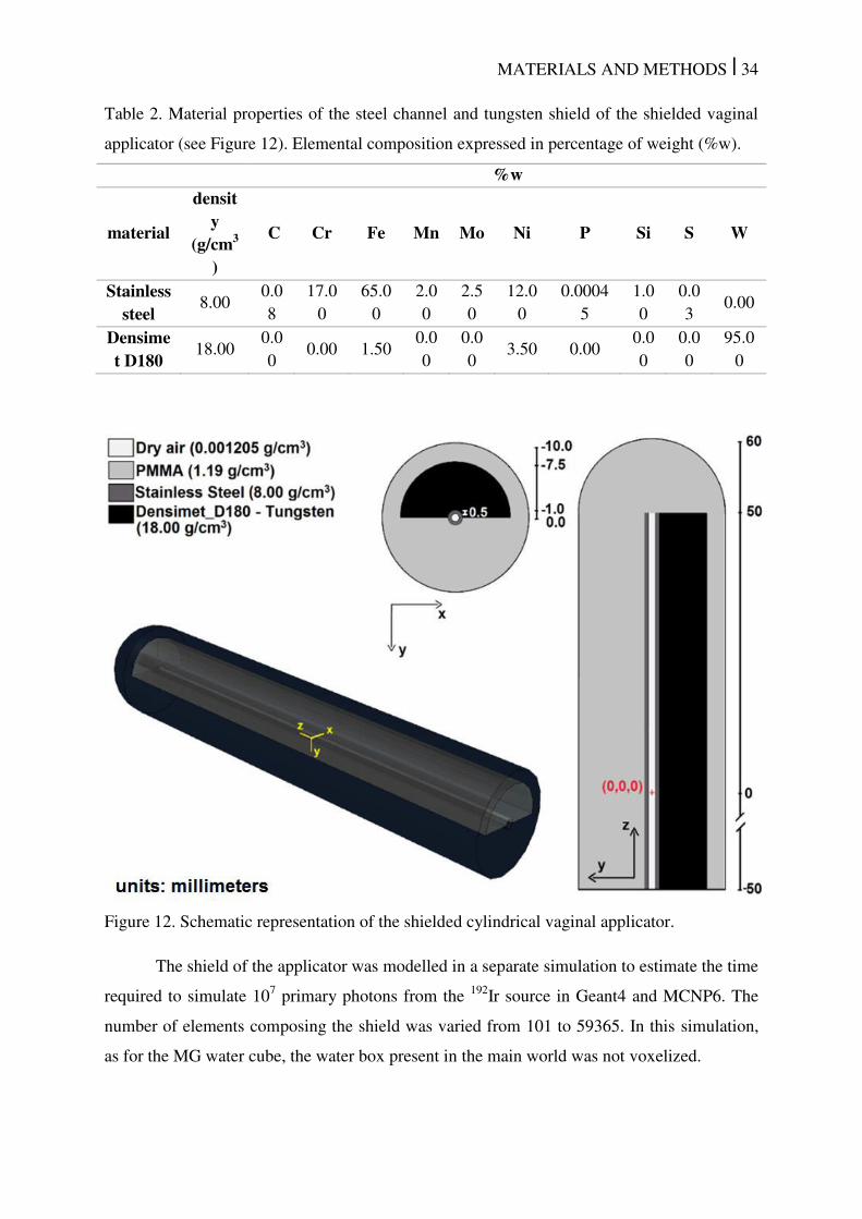
MATERIALS AND METHODS | 34
Table 2. Material properties of the steel channel and tungsten shield of the shielded vaginal
applicator (see Figure 12). Elemental composition expressed in percentage of weight (%w).
%w
material
density
(g/cm3
)
C Cr Fe Mn Mo Ni P Si S W
Stainless steel
8.00 0.0
8
17.0
0
65.0
0
2.0
0
2.5
0
12.0
0
0.0004
5
1.0
0
0.0
3 0.00
Densimet D180
18.00 0.0
0 0.00 1.50
0.0
0
0.0
0 3.50 0.00
0.0
0
0.0
0
95.0
0
Figure 12. Schematic representation of the shielded cylindrical vaginal applicator.
The shield of the applicator was modelled in a separate simulation to estimate the time
required to simulate 107 primary photons from the
192Ir source in Geant4 and MCNP6. The
number of elements composing the shield was varied from 101 to 59365. In this simulation,
as for the MG water cube, the water box present in the main world was not voxelized.
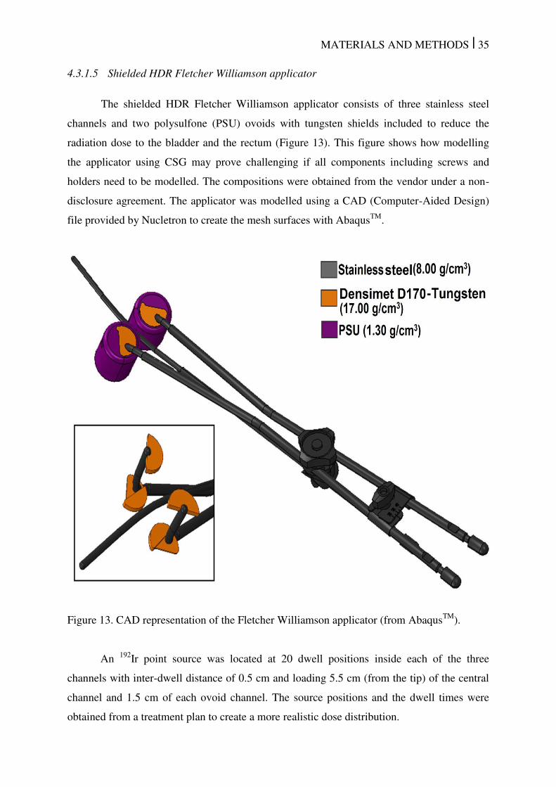
MATERIALS AND METHODS | 35
4.3.1.5 Shielded HDR Fletcher Williamson applicator
The shielded HDR Fletcher Williamson applicator consists of three stainless steel
channels and two polysulfone (PSU) ovoids with tungsten shields included to reduce the
radiation dose to the bladder and the rectum (Figure 13). This figure shows how modelling
the applicator using CSG may prove challenging if all components including screws and
holders need to be modelled. The compositions were obtained from the vendor under a non-
disclosure agreement. The applicator was modelled using a CAD (Computer-Aided Design)
file provided by Nucletron to create the mesh surfaces with AbaqusTM
.
Figure 13. CAD representation of the Fletcher Williamson applicator (from AbaqusTM
).
An 192
Ir point source was located at 20 dwell positions inside each of the three
channels with inter-dwell distance of 0.5 cm and loading 5.5 cm (from the tip) of the central
channel and 1.5 cm of each ovoid channel. The source positions and the dwell times were
obtained from a treatment plan to create a more realistic dose distribution.
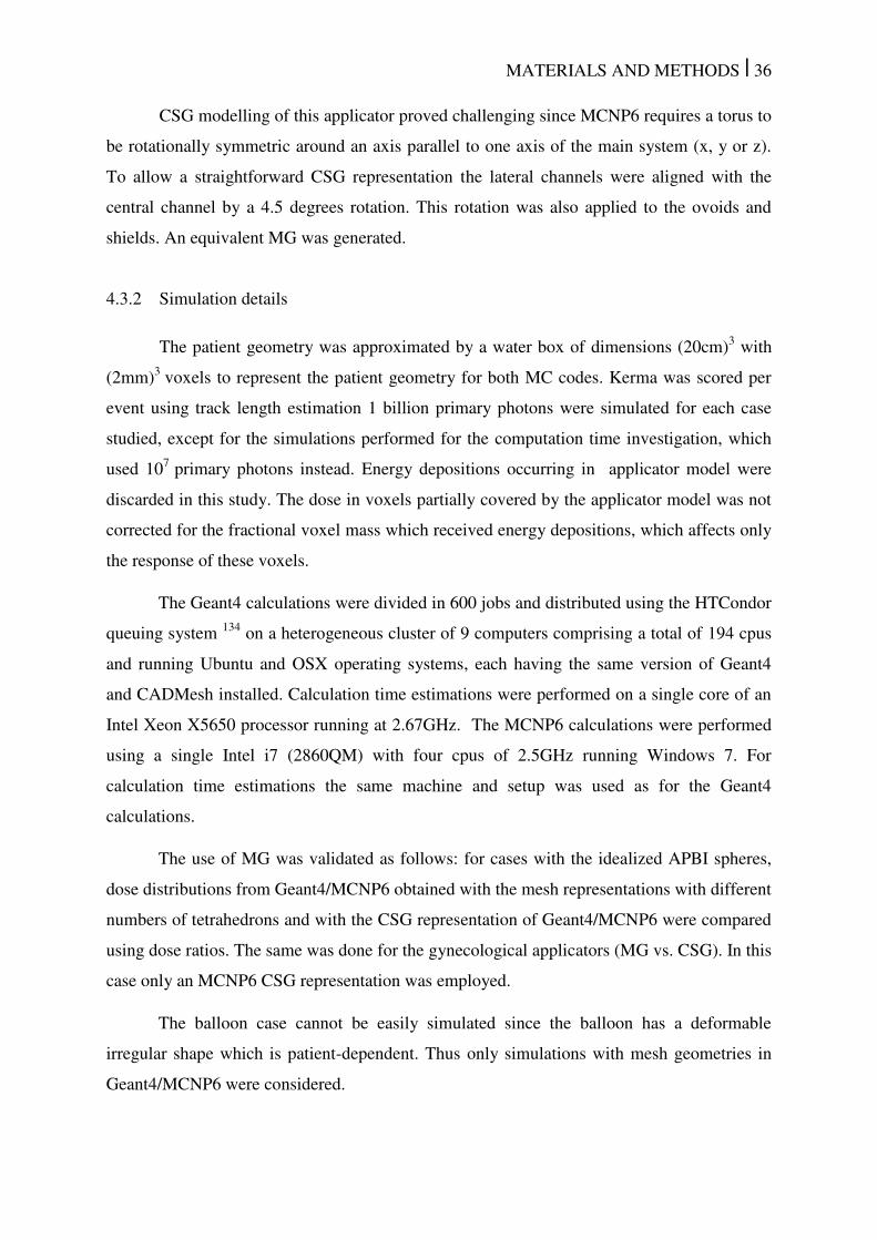
MATERIALS AND METHODS | 36
CSG modelling of this applicator proved challenging since MCNP6 requires a torus to
be rotationally symmetric around an axis parallel to one axis of the main system (x, y or z).
To allow a straightforward CSG representation the lateral channels were aligned with the
central channel by a 4.5 degrees rotation. This rotation was also applied to the ovoids and
shields. An equivalent MG was generated.
4.3.2 Simulation details
The patient geometry was approximated by a water box of dimensions (20cm)3 with
(2mm)3
voxels to represent the patient geometry for both MC codes. Kerma was scored per
event using track length estimation 1 billion primary photons were simulated for each case
studied, except for the simulations performed for the computation time investigation, which
used 107
primary photons instead. Energy depositions occurring in applicator model were
discarded in this study. The dose in voxels partially covered by the applicator model was not
corrected for the fractional voxel mass which received energy depositions, which affects only
the response of these voxels.
The Geant4 calculations were divided in 600 jobs and distributed using the HTCondor
queuing system 134
on a heterogeneous cluster of 9 computers comprising a total of 194 cpus
and running Ubuntu and OSX operating systems, each having the same version of Geant4
and CADMesh installed. Calculation time estimations were performed on a single core of an
Intel Xeon X5650 processor running at 2.67GHz. The MCNP6 calculations were performed
using a single Intel i7 (2860QM) with four cpus of 2.5GHz running Windows 7. For
calculation time estimations the same machine and setup was used as for the Geant4
calculations.
The use of MG was validated as follows: for cases with the idealized APBI spheres,
dose distributions from Geant4/MCNP6 obtained with the mesh representations with different
numbers of tetrahedrons and with the CSG representation of Geant4/MCNP6 were compared
using dose ratios. The same was done for the gynecological applicators (MG vs. CSG). In this
case only an MCNP6 CSG representation was employed.
The balloon case cannot be easily simulated since the balloon has a deformable
irregular shape which is patient-dependent. Thus only simulations with mesh geometries in
Geant4/MCNP6 were considered.
MATERIALS AND METHODS | 37
4.4 Dose specification (Dw,m and Dm,,m)
This section describes the evaluated clinical case, simulation parameters and the
methodology employed to convert Dm,m to Dw,m using SCT and LCT.
4.4.1 Clinical case
The treatment plan for an interstitial clinical head and neck case was made with a CT
image set consisting of 80 slices with 512x512 voxels (0.39x0.39x2.00 mm3). Dose
distributions were calculated for a HDR 192
Ir microSelectron v.2 (Nucletron) source 76, 77
and
six plastic catheters with a total of 99 dwell positions. 25 CT voxels were visually selected to
evaluate the photon spectrum at several regions of the irradiated volume occupied by
different materials and at different distances from implanted sources. The patient CT
geometry and the location of the 25 voxels for which the photon spectrum was scored (see the
next section) are shown in Figure 14.
Figure 14. Axial and sagittal view of the evaluated head and neck clinical case. The numbers
indicate voxels positions where the photon spectrum was scored. Green arrows and squares
were added to show the catheter positions (five of the six catheters can be visualized).
4.4.2 Monte Carlo simulations
The CT images were segmented using auxiliary software 135
to create three voxel
phantoms including: I - a water (ρ = 1 g/cm3) and air (ρ = 0.0012 g/cm3) phantom; II - a water
and air phantom with mass densities obtained from a calibrated CT image; III - a phantom
MATERIALS AND METHODS | 38
with proper tissue compositions (adipose tissue, muscle and bone) 129
, with mass densities
obtained from a calibrated CT image. The regions with air are the same for all models
adopted so henceforward this material will not be mentioned anymore when referring to the
described phantoms. These phantoms were employed to evaluate the effect of different
approaches/simplifications that can be easily adopted by MC users. Moreover, Dw,w values
obtained with phantom II were compared (data not shown) against Dw,m (LCT) and Dm,m
values obtained with phantom III since using phantom II is simpler, but may still provide
reasonable results. The numbers (I, II and III) were used in the next sections to distinguish the
three different approaches.
Simulations were performed with MCNP6 for the three phantoms, scoring in all
voxels the mean photon energy per voxel, Dw,m (LCT) and Dm,m and for the 25 selected
voxels the full photon energy spectra with a 1 keV resolution (Figure 14). Dw,m (LCT) and
Dm,m values were obtained using a track length estimator (tally F6) assuming CPE conditions
so secondary electrons were not transported (see next section). Mass-energy absorption
coefficients (µen/) from the National Institute of Standards and Technology (NIST)114
for
either water or medium were employed to convert photon energy fluence to collision kerma
(equal to absorbed dose under CPE). In addition, Dm,m values were calculated transporting
secondary electrons and using a pulse height tally (F8) to verify Dm,m obtained with a track
length tally F6 to study the validity of the CPE approximation on the dosimetry (and thus on
using a track length estimator for this kind of geometries) on the current dose calculation
voxel grid. Earlier investigations confirmed the validity of CPE using even smaller voxels
(0.1x0.1x0.1 mm3),
118 but studied the problem outside a brachytherapy source positioned in
pure water to estimate the importance of modelling charged particles emitted in the source
decay. CPE conditions are achieved for the 192
Ir spectrum for distances greater than 2 mm
from the source.118, 119
However, breakdown of CPE can occur near material boundaries.13
The effect of the interfaces between different materials and their influence on the CPE
assumption has not been studied before in a CT defined phantom with voxel dimensions as
those adopted in this study.
The number of primary photons (N) was set to 1 billion (109) for the mean energy
simulation, 10 billion for the track length and photon spectrum simulations, and 30 billion for
pulse height tally simulation.
MATERIALS AND METHODS | 39
4.4.3 Dw,m (SCT and LCT) and Dm,m values for several tissues
The photon spectrum in the 25 selected voxels was used with materials encountered in
the head and neck region, but also with some other materials. Dw,m (LCT), Dm,m and mean
photon energy values were obtained for several human tissues (prostate, lung, adipose tissue,
breast, skin, bladder, muscle, cartilage, mandible spongiosa, bone and teeth)129
with the full
photon spectrum obtained at the 25 evaluated voxels. The contribution of separate parts of
the photon spectrum to the total dose in each voxel was obtained by dividing the spectrum in
50 keV bins and calculating the percentage of the total dose from each bin.
Dw,m (SCT) were obtained for each material assuming /� � to be independent of
the photon spectrum (Figure 1.b). Conversion coefficients were obtained using the ESTAR
database 40
averaging /� � values with energies between 0.010 MeV and 1.5 MeV since
electron spectra were not simulated for the evaluated clinical case.
4.5 Transit dose
The dwell positions and the catheter contours can be imported from the
BrachyVisionTM
and the OncentraTM
TPS, consisting of point coordinates related to the
treatment plan geometry. These points were used to define the trajectory of the source inside
the patient and its inclination. The length of the catheter and the number of contour points
depend on the catheter contouring process and the number of segments created to define the
source trajectory in the treatment plan, or, alternatively, on the method of defining the
applicator in the TPS applicator library. The catheter points and the dwell positions were
processed using an algorithm created with MATLAB version 8.0, which provides the
trajectory of the source, the speed at each reference position, control points where the
acceleration changes direction, the source orientation and the time necessary to travel
between two consecutive points for both the source going into the patient and coming back to
the safe.
The trajectory depends of the treatment plan and is mainly restricted to the region near
to the target volume since the catheters outside of the body, in general, are not defined when
planning. However, this is not a limitation for this study since its main interest is the transit
dose due to the source travel between dwell positions, with a low speed near the dwell
positions as shown in section 4.5.2 Validation.

MATERIALS AND METHODS | 40
4.5.1 Transit dose calculation
The transit dose distribution due to the source traveling inside the patient, without
considering the dwell time, and the dwell dose distribution were obtained separately for 4
clinical cases using the MCNP5 MC code. The transit dose and the dwell dose was evaluated
using a phase space file, which was generated on the surface of the stainless steel capsule
encasing the 192
Ir isotope considering a 2 mm long cable. Since the goal was to analyze the
transit dose component and the effect of several speed profiles, all the cases were simulated
under the same conditions using a microSelectron v.2 source that was validated by simulating
TG43-U11, 2
parameters in a 30 cm diameter water phantom following the methodology
proposed by Daskalov et al.77
This approach ensures that differences between the cases are
not due to the source model. The simulations were performed with 109 photons resulting in a
dose uncertainty component type A (k=1) of less than 1.5% for points with a dose higher than
10% of the prescribed dose.
The MC transit dose calculations for the clinical cases simulate the source at discrete
positions every 10 µm following the source trajectory with a sampling probability defined as
the inverse of the instantaneous speed along the trajectory, which is proportional to the time
spent by the source to travel within each 10 µm segment for the source going into the patient,
traveling between the dwell positions and coming back to the safe. The discrete methodology
should be equivalent to a continuous distribution due to the high spatial resolution adopted,
which was evaluated using a continuous and a discrete distribution for a point source
following a straight trajectory. This methodology was employed in a previous study41
where
simulated data was also validated by comparison against experimental values obtained by
Calcina et al.136
This study adopted a maximum source instantaneous speed of 52 cm/s (ref. 46) with
the instantaneous source speed at each position calculated using reference speeds and
accelerations from the literature following the three approaches: a) uniform acceleration; b)
an average speed obtained considering the inter-dwell distance and the travel time, which was
obtained using the source acceleration; c) the average speed of 30 cm/s and 50 cm/s specified
by two manufacturers. The average speed values provided by the manufacturers do not
depend on the inter-dwell distance and may not refer to the speed between the dwell
positions, depending on the measurement methodology, although these speed values can be
used as reference values. Nucletron suggests dwell time corrections using an average speed of
MATERIALS AND METHODS | 41
50 cm/s for a 5 mm inter-dwell distance.137
This dwell time correction was not considered for
the evaluated clinical cases and was described in sections 4.6 and 5.5 (Speed measurements).
4.5.2 Validation
The MC source distribution for the clinical cases simulates the source at each
position, which is equivalent to the superposition principle used to validate simulation results
for simplified cases. While the studied cases were evaluated accounting for the anisotropy,
scattering and other interactions, the validation process was performed using an isotropic
point source and the superposition technique which can be verified with simple dose
calculation algorithms. The validation process consists of three steps:
a) speed profile verification by comparing the speed profile calculated using the
TPS contour information and obtained analytically;
b) MC simulation of the transit dose component versus a calculation using
MATLAB for a treatment plan created for a point source and a linear 10 cm long
catheter with dwell positions distributed uniformly along it for inter-dwell
distances of 2.5 mm, 5.0 mm, 10.0 mm and 20 mm. This is illustrated in Figure
15 for a simplified case with 3 dwell positions;
c) creation of a treatment plan for a ring applicator with 32 mm of diameter defined
in the BrachyVisionTM
applicators library (ref: AL13017000) with inter-dwell
distance of 0.5 cm used only to verify the source trajectory. The transit dose
distribution was simulated considering the source instantaneous speed, and then
exported back to the TPS as DICOM images allowing a visualization of the
applicator and the dwell positions superimposed over the transit dose distribution.
The transit dose component for one reference point (Ref-1; Figure 15.a) was
estimated considering a trajectory composed by N steps of 10 µm with travel times calculated
using a source instantaneous speed profile (Figure 15.b). The contribution of each step along
the trajectory to the total transit dose at the reference point (Ref-1/ Figure 15.a) is
proportional to the travel time of each step weighted by the square of the distance d’ between
the position of the center of the 10 m step and the reference point to take into account the
inverse-square law resulting in the distribution presented in Figure 15.c. Finally, the transit
dose component ( � was obtained by integrating the obtained distribution and multiplying
it by the dose rate ( for an arbitrary reference distance � as described in the following
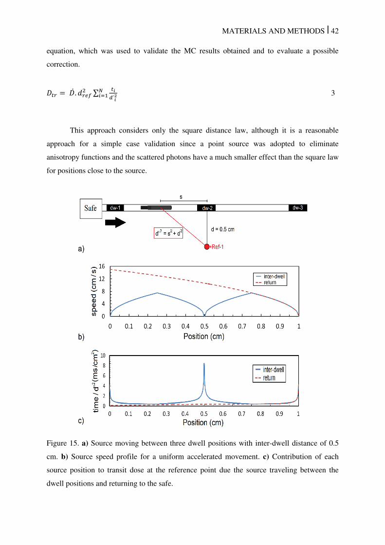
MATERIALS AND METHODS | 42
equation, which was used to validate the MC results obtained and to evaluate a possible
correction.
� = . � ∑ ��2��= 3
This approach considers only the square distance law, although it is a reasonable
approach for a simple case validation since a point source was adopted to eliminate
anisotropy functions and the scattered photons have a much smaller effect than the square law
for positions close to the source.
Figure 15. a) Source moving between three dwell positions with inter-dwell distance of 0.5
cm. b) Source speed profile for a uniform accelerated movement. c) Contribution of each
source position to transit dose at the reference point due the source traveling between the
dwell positions and returning to the safe.
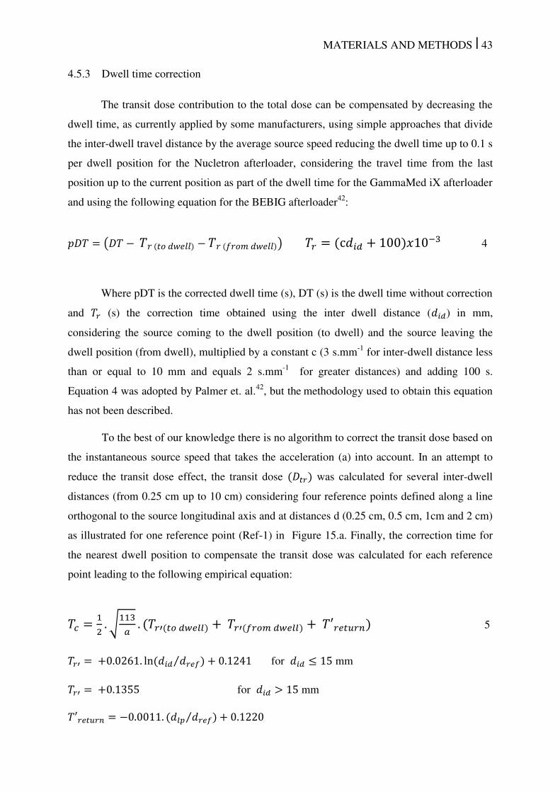
MATERIALS AND METHODS | 43
4.5.3 Dwell time correction
The transit dose contribution to the total dose can be compensated by decreasing the
dwell time, as currently applied by some manufacturers, using simple approaches that divide
the inter-dwell travel distance by the average source speed reducing the dwell time up to 0.1 s
per dwell position for the Nucletron afterloader, considering the travel time from the last
position up to the current position as part of the dwell time for the GammaMed iX afterloader
and using the following equation for the BEBIG afterloader42
:
= ( − � � − � � ) � = c � + − 4
Where pDT is the corrected dwell time (s), DT (s) is the dwell time without correction
and � (s) the correction time obtained using the inter dwell distance ( � ) in mm,
considering the source coming to the dwell position (to dwell) and the source leaving the
dwell position (from dwell), multiplied by a constant c (3 s.mm-1
for inter-dwell distance less
than or equal to 10 mm and equals 2 s.mm-1
for greater distances) and adding 100 s.
Equation 4 was adopted by Palmer et. al.42
, but the methodology used to obtain this equation
has not been described.
To the best of our knowledge there is no algorithm to correct the transit dose based on
the instantaneous source speed that takes the acceleration (a) into account. In an attempt to
reduce the transit dose effect, the transit dose � was calculated for several inter-dwell
distances (from 0.25 cm up to 10 cm) considering four reference points defined along a line
orthogonal to the source longitudinal axis and at distances d (0.25 cm, 0.5 cm, 1cm and 2 cm)
as illustrated for one reference point (Ref-1) in Figure 15.a. Finally, the correction time for
the nearest dwell position to compensate the transit dose was calculated for each reference
point leading to the following empirical equation:
= . √ � . �′ � + �′ � � + ′� � 5
�′ = + . . ln � �⁄ + . for � ≤ mm
�′ = + . for � > mm ′� � = − . . �⁄ + .
MATERIALS AND METHODS | 44
where the correction time ( in s, that should be subtracted from the TPS dwell time of the
nearest dwell position. depends on the reference distance ( � ), 1 mm, the inter-dwell
distances ( � in mm and the distance between the current and the last position ( in mm.
Equation 5 includes the source coming from the previous position or from the safe to
the current dwell position, �′ � in s. The latter is approximated as an inter-dwell
distance of 100 mm, Tc also depends on the source going from the current position to the next
dwell position, �′ � � in s, and the source returning to the safe, ′� � in s. The
factor 1/2 was included since the transit time in one inter-dwell segment will be corrected for
two consecutive dwell positions and the factor (113/a)1/2
includes the acceleration effect since
the time of each discrete step is inversely proportional to the square root of the ratio of the
reference acceleration (113 cm/s2) and the acceleration (a) as obtained from kinematics and
evaluated for accelerations (�) between 10 cm/s2 and 200 cm/s
2 to cover the literature data
interval.
The described approach compensates the transit dose effect, includes the acceleration
and preserves the simplicity of the manufacturer’s approaches. Although our approach
includes the acceleration component, as the currently available algorithms it cannot
completely correct the transit dose due to the limited number and location of the dwell
positions. Moreover, complex transit dose distributions may occur, e.g. due to different inter-
dwell distances in the same setup and/or due to the geometry and the number of catheters.
4.5.4 Clinical cases
Two gynecological cases and one prostate case were planned for a microSelectron-
HDR 192
Ir source77
using the TG-43U1 dose while one prostate case was planned for a
GamammedPlus source76
. These cases were selected to provide a general overview of the
transit dose component since they differ considerably in the number of catheters, inter-dwell
distance and geometry. Regardless of the differences between the source, all the cases were
simulated using the microSelectron HDR source with the dwell times of each case scaled to
an air-kerma strength of 40700 U in order to evaluate all cases under the same air-kerma
strength and also to evaluate the worst case scenario since the transit dose is directly
proportional to this parameter. Simulations were performed for two situations: a) an infinite
water medium, which was created by adding at least 20 cm of water at each side of the
body;130
b) a heterogeneous medium composed of five materials, air (mass density ρ =
MATERIALS AND METHODS | 45
0.0012041 g/cm3), water (ρ = 1.0 g/cm3), adipose tissue (ρ = 0.92 g/cm3), muscle (ρ = 1.06
g/cm3) and cortical bone (ρ = 1.85 g/cm3
) defined using Hounsfield units (HU) with
compositions defined by the International Commission on Radiological Protection (ICRP-
1975).138
One density was specified for each material to assure that MCNP5 uses the same
composition and density specified using ACUROS™, a grid based Boltzmann solver, which
was used, in a parallel work, to validate the dose distributions without the transit dose. The
cases were compared considering the 3D dose distributions and also by comparing doses at
prescription points defined by the physician responsible for the case, since structure contours
were not created for all the cases.
Dw,m (dose to water in medium) values were obtained for all cases and only the values
obtained for an infinite water phantom are presented, except when stated otherwise, since the
transit dose component relative to the dwell dose is the same for all the conditions evaluated.
4.5.5 Gynecological cases
Two gynecological cases differing significantly in the number of needles and dwell
positions were selected to evaluate the impact of the number of needles and their locations.
The evaluated cases were: case a) a treatment performed with a hollow cylindrical vaginal
applicator with an external diameter of 35 mm and a polysulfone wall of 4 mm with one 12
cm long needle in the center totaling 17 dwell positions, inter-dwell distance of 2.5 mm and a
total dwell time of 405 s. The reference points were defined at a distance of 5 mm from the
right hand side of the applicator wall with an average dose of 7 Gy; case b) a treatment
performed with the same applicator described in the previous case using the central needle of
the applicator and three needles distributed near the lower surface of the applicator totaling
100 dwell positions and a total dwell time of 556 s. Each needle has been defined during the
treatment planning with approximately 12 cm of contour length and an inter-dwell distance of
2.5 mm. The reference dose points were defined on the right hand side of the applicator’s
surface with an average dose of 15 Gy.
4.5.6 Prostate cases
Two prostate cases were selected, which had approximately the same total dwell time
and prescribed dose, but a significantly different number and distribution of the needles. The
evaluated cases were: case c) a treatment performed using 16 flexible catheters with lengths
defined through contours during the planning between 3.8 cm and 6.3 cm, the number of
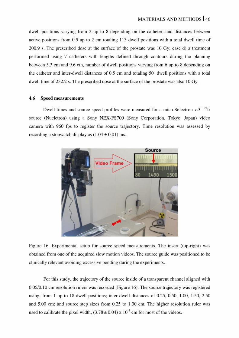
MATERIALS AND METHODS | 46
dwell positions varying from 2 up to 8 depending on the catheter, and distances between
active positions from 0.5 up to 2 cm totaling 113 dwell positions with a total dwell time of
200.9 s. The prescribed dose at the surface of the prostate was 10 Gy; case d) a treatment
performed using 7 catheters with lengths defined through contours during the planning
between 5.3 cm and 9.6 cm, number of dwell positions varying from 6 up to 8 depending on
the catheter and inter-dwell distances of 0.5 cm and totaling 50 dwell positions with a total
dwell time of 232.2 s. The prescribed dose at the surface of the prostate was also 10 Gy.
4.6 Speed measurements
Dwell times and source speed profiles were measured for a microSelectron v.3 192
Ir
source (Nucletron) using a Sony NEX-FS700 (Sony Corporation, Tokyo, Japan) video
camera with 960 fps to register the source trajectory. Time resolution was assessed by
recording a stopwatch display as (1.04 ± 0.01) ms.
Figure 16. Experimental setup for source speed measurements. The insert (top-right) was
obtained from one of the acquired slow motion videos. The source guide was positioned to be
clinically relevant avoiding excessive bending during the experiments.
For this study, the trajectory of the source inside of a transparent channel aligned with
0.05/0.10 cm resolution rulers was recorded (Figure 16). The source trajectory was registered
using: from 1 up to 18 dwell positions; inter-dwell distances of 0.25, 0.50, 1.00, 1.50, 2.50
and 5.00 cm; and source step sizes from 0.25 to 1.00 cm. The higher resolution ruler was
used to calibrate the pixel width, (3.78 ± 0.04) x 10
-3 cm for most of the videos.
MATERIALS AND METHODS | 47
Source positions were evaluated frame-by-frame with in-house software developed
using MATLAB version 8.0. The region of interest (ROI) that represents the source trajectory
was manually assigned and then the pixel intensity profile, without the source, was recorded
as the background profile (BG). Source structures (e.g. the tip and the welding) can be easily
identified dividing the pixel intensity profile inside the ROI of each frame by the BG profile
as illustrated by the top right figure in video 1.**
This video shows the software used to track
the source, the source movement and intensity profiles including reference lines, with fixed
distances between them, associated with source structures. These lines were included to
verify possible misdetections. Average speeds were calculated over three measurements.
All speed values were averaged over distance intervals of 0.2 cm ( . ), except when
otherwise stated. The dwell-time correction applied by the afterloader was measured for all
setups by comparing the programmed dwell time against the dwell time recorded using the
video footage. Dwell-times were measured after the source comes to rest at the specified
dwell position.
The source trajectory between two consecutive dwell positions starts with the source
leaving the first dwell position and ends immediately before the source reaching the second
dwell position for the first time. We noticed that, after the source reaches a dwell position it
overshoots and oscillates around it, an effect that was not considered for the average speed
determination. The duration the source spends oscillating around a dwell position was
measured.
4.6.1 Experimental uncertainty
Two types of uncertainties were adopted: Type A – standard deviation (±1σ) of the
results obtained repeating the experiments; Type B – defined as two pixels width and half of
the time resolution. The uncertainty on the time is 5.2x10⁻⁴
s while the uncertainty on the
source position is 7.56x10⁻³
cm. All speed values obtained over 0.2 cm intervals have an
uncertainty component of 3.8% for the distance while the average speed over larger inter-
dwell distances has a smaller relative uncertainty component for the distance. The uncertainty
component due to the time resolution varies considerably due to the number of frames
** Videos available online: ftp://ftp.aip.org/epaps/med_phys/E-MPHYA6-42-018501
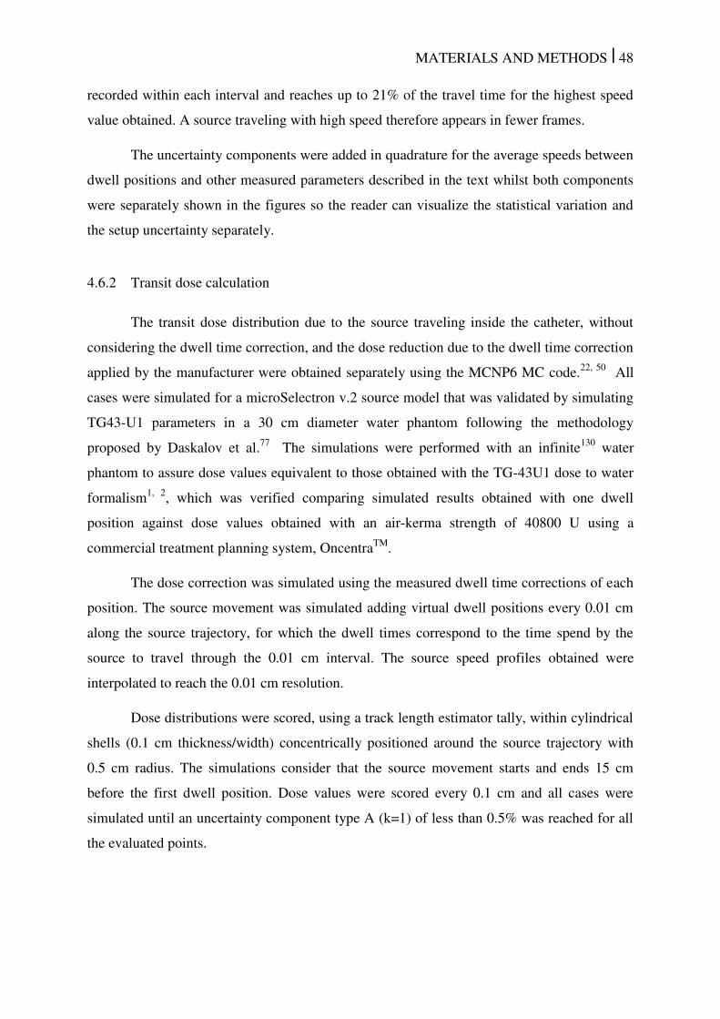
MATERIALS AND METHODS | 48
recorded within each interval and reaches up to 21% of the travel time for the highest speed
value obtained. A source traveling with high speed therefore appears in fewer frames.
The uncertainty components were added in quadrature for the average speeds between
dwell positions and other measured parameters described in the text whilst both components
were separately shown in the figures so the reader can visualize the statistical variation and
the setup uncertainty separately.
4.6.2 Transit dose calculation
The transit dose distribution due to the source traveling inside the catheter, without
considering the dwell time correction, and the dose reduction due to the dwell time correction
applied by the manufacturer were obtained separately using the MCNP6 MC code.22, 50
All
cases were simulated for a microSelectron v.2 source model that was validated by simulating
TG43-U1 parameters in a 30 cm diameter water phantom following the methodology
proposed by Daskalov et al.77
The simulations were performed with an infinite130
water
phantom to assure dose values equivalent to those obtained with the TG-43U1 dose to water
formalism1, 2
, which was verified comparing simulated results obtained with one dwell
position against dose values obtained with an air-kerma strength of 40800 U using a
commercial treatment planning system, OncentraTM
.
The dose correction was simulated using the measured dwell time corrections of each
position. The source movement was simulated adding virtual dwell positions every 0.01 cm
along the source trajectory, for which the dwell times correspond to the time spend by the
source to travel through the 0.01 cm interval. The source speed profiles obtained were
interpolated to reach the 0.01 cm resolution.
Dose distributions were scored, using a track length estimator tally, within cylindrical
shells (0.1 cm thickness/width) concentrically positioned around the source trajectory with
0.5 cm radius. The simulations consider that the source movement starts and ends 15 cm
before the first dwell position. Dose values were scored every 0.1 cm and all cases were
simulated until an uncertainty component type A (k=1) of less than 0.5% was reached for all
the evaluated points.

RESULTS AND DISCUSSIONS
Chapter 5
RESULTS AND DISCUSSIONS | 50
5 RESULTS AND DISCUSSIONS
5.1 AMIGOBrachy
AMIGOBrachy employs a user-friendly user interface, obviating any technical
MCNP6 knowledge, thus considerably reducing the time necessary to process the treatment
data and to perform a MC simulation. Figure 17 presents a few screenshots of
AMIGOBrachy with the ImageView module, 3D images and dose distributions. As an
example, a patient CT slice, a rendered organ and a few dose distributions are shown.
Figure 17. AMIGOBrachy screenshots of a) AMIGOBrachy ImageView module; b) 3D
rendering of lungs; c) dose distribution of a single source dwell position with dose profiles; d)
dose distribution obtained using a titanium fletcher applicator and a sequence of source dwell
positions.
RESULTS AND DISCUSSIONS | 51
5.1.1 Uniform Phantoms Validation
Dwell positions in AMIGOBrachy showed no differences from TPS values, indicating
AMIGOBrachy correctly imports the values from the TPS. Errors in the dwell positions were
manually introduced, which led to clearly visible differences in the dose ratios even for
positioning differences smaller than 0.5 mm. Therefore, source mispositioning problems can
be easily detected. Calculated TG43-U1 parameters1, 2
for the source are in good agreement
with literature parameters with most of the points showing less than a 1% dose difference.
For GammaMed Plus more than 90% and 99% of the anisotropy function values show
agreement with Taylor et al.76
within 1% and 2%, respectively.
Results for the water cube phantom with AMIGOBrachy/MCNP6 and ACUROSTM
are in good agreement for all dose scoring grids. However, the agreement is affected by the
scoring grid resolution since 95% of the voxel doses agree within 0.6, 1.0, 2.2 and 3.2% for
scoring grid widths and heights of 5.0, 2.5, 1.0 and 0.5 mm. Uncertainty values are larger for
smaller water voxel sizes since all simulations were performed with the same number of
primary photons. In addition, ACUROSTM
solves the Boltzmann transport equation by
discretizing its six variables11, 18, 128
leading to some discretization artifacts that become
visible with higher dose grid resolution. The mean dose per slice, obtained for statistic
reasons, for the evaluated grid sizes were compared against the 1 mm3 grid. Differences
lower than ±0.2% were observed for all.
Results obtained with phantoms of different materials (data not shown) were also
compared using the mean dose per slice. The agreement between AMIGOBrachy/MCNP6
and ACUROSTM
is the same for all tissues with mean differences per slice within ±0.3%
when compared against values obtained with a water phantom. The ratio of the mean dose per
slice was visually evaluated and no systematic differences were found.
5.1.2 Clinical Cases Validation
The results obtained with AMIGOBrachy/MCNP6 for both patient cases were in good
agreement with the values calculated with ACUROSTM
, with differences of less than 2% and
5% for more than 92% and 98% of voxels with doses higher than 10% of the prescribed dose,
respectively. Larger differences were observed in regions with a dose below 10% of the
prescribed dose, which were due to the statistical uncertainty of the simulation. Figure 18
shows the results obtained including a 3D CT view (top), the dose ratio between ACUROSTM
RESULTS AND DISCUSSIONS | 52
and MCNP6 (middle) and the dose ratio of MCNP6 for a homogeneous water medium and
the proper material compositions (bottom).
The agreement between MCNP6 calculations for the intracavitary case performed
using an applicator defined analytically and ACUROSTM
is slightly lower than the agreement
obtained using voxels for both codes with 87% of the voxels with differences below 2%. This
is due to the differences in the gynecological applicator position and model since the
analytical model of the applicator (MC) was compared against a voxel model. It was not
possible to include the applicator in the ACUROSTM
applicator database leading to different
models, similar to the illustration in Figure 8 for another applicator.
The intracavitary case shows isodose displacements of about 1 mm and dose
differences of around 5% in the region within the 100% isodose, which is mostly due to the
hollow applicator effect since no significant difference was observed in the simulations
modelling water or the actual tissue composition. The effect of the soft tissue composition
and density is less than 1% for soft tissue, with no significant isodose displacement. The
effect of the finite body dimensions is also visible in Figure 18.c1 showing increasing
differences towards the boundaries of the body. This represents a lower dose obtained with
MCNP6 since the air around the body reduces the number of backscattered photons, which is
neglected by the TG-43U1 formalism.
The interstitial case also shows significant dose differences when MCNP6 is used
with tissue heterogeneities and uniform water. Isodose displacements were obtained up to 1.6
mm and 4.1 mm for the 100% and 50% isodoses, respectively. Inside the 100% isodose the
underdose using proper tissue composition is about 5% with differences increasing towards
the outer surface of the arm. The effect of the soft tissue composition and density is less than
1%. The bone medium yields displacements of up to 4.0 mm in the 100% isodose at some
points behind this material.
5.1.3 Clinical applicability
The simulation efficiency depends on the clinical case with potentially significant
differences since the effects of LSTE and geometrical optimization can depend on the case
and on the user-defined parameters. The size of the region that is voxelized (Figure 9.d) also
influences both efficiency and accuracy.

RESULTS AND DISCUSSIONS | 53
Figure 18. Results for the two patient geometries: the intracavitary gynecological case (left
panels) and the interstitial arm case (right panels). a) 3D view indicating the assigned
materials. b) Isodoses and dose ratio ACUROSTM
/MCNP6. c) Isodoses and dose ratio
MCNP6(homogeneous water)/MCNP6(heterogeneous geometry).
Simulations using the track length estimator tally (MCNP6 F6) with the LSTE
function disabled required at least 100 times longer calculation times than those performed
using FMESH (virtual grid based track length estimator tally) with the LSTE function
activated. This result agreed with the LSTE description and was performed only for one case
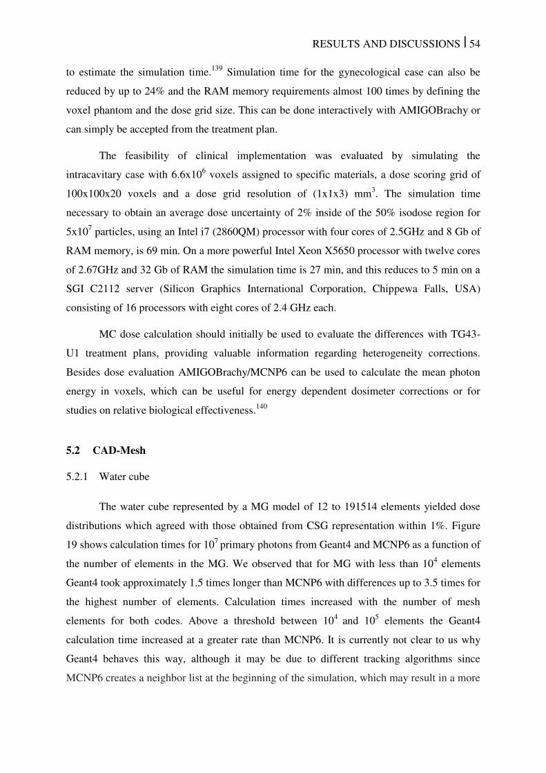
RESULTS AND DISCUSSIONS | 54
to estimate the simulation time.139
Simulation time for the gynecological case can also be
reduced by up to 24% and the RAM memory requirements almost 100 times by defining the
voxel phantom and the dose grid size. This can be done interactively with AMIGOBrachy or
can simply be accepted from the treatment plan.
The feasibility of clinical implementation was evaluated by simulating the
intracavitary case with 6.6x10⁶ voxels assigned to specific materials, a dose scoring grid of
100x100x20 voxels and a dose grid resolution of (1x1x3) mm3. The simulation time
necessary to obtain an average dose uncertainty of 2% inside of the 50% isodose region for
5x10⁷ particles, using an Intel i7 (2860QM) processor with four cores of 2.5GHz and 8 Gb of
RAM memory, is 69 min. On a more powerful Intel Xeon X5650 processor with twelve cores
of 2.67GHz and 32 Gb of RAM the simulation time is 27 min, and this reduces to 5 min on a
SGI C2112 server (Silicon Graphics International Corporation, Chippewa Falls, USA)
consisting of 16 processors with eight cores of 2.4 GHz each.
MC dose calculation should initially be used to evaluate the differences with TG43-
U1 treatment plans, providing valuable information regarding heterogeneity corrections.
Besides dose evaluation AMIGOBrachy/MCNP6 can be used to calculate the mean photon
energy in voxels, which can be useful for energy dependent dosimeter corrections or for
studies on relative biological effectiveness.140
5.2 CAD-Mesh
5.2.1 Water cube
The water cube represented by a MG model of 12 to 191514 elements yielded dose
distributions which agreed with those obtained from CSG representation within 1%. Figure
19 shows calculation times for 107
primary photons from Geant4 and MCNP6 as a function of
the number of elements in the MG. We observed that for MG with less than 104 elements
Geant4 took approximately 1.5 times longer than MCNP6 with differences up to 3.5 times for
the highest number of elements. Calculation times increased with the number of mesh
elements for both codes. Above a threshold between 104
and 105 elements the Geant4
calculation time increased at a greater rate than MCNP6. It is currently not clear to us why
Geant4 behaves this way, although it may be due to different tracking algorithms since
MCNP6 creates a neighbor list at the beginning of the simulation, which may result in a more
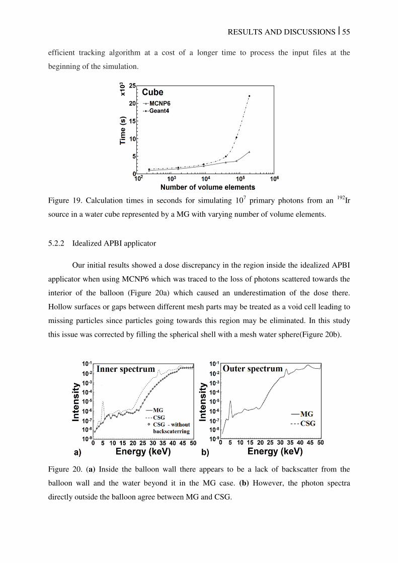
RESULTS AND DISCUSSIONS | 55
efficient tracking algorithm at a cost of a longer time to process the input files at the
beginning of the simulation.
Figure 19. Calculation times in seconds for simulating 107 primary photons from an
192Ir
source in a water cube represented by a MG with varying number of volume elements.
5.2.2 Idealized APBI applicator
Our initial results showed a dose discrepancy in the region inside the idealized APBI
applicator when using MCNP6 which was traced to the loss of photons scattered towards the
interior of the balloon (Figure 20a) which caused an underestimation of the dose there.
Hollow surfaces or gaps between different mesh parts may be treated as a void cell leading to
missing particles since particles going towards this region may be eliminated. In this study
this issue was corrected by filling the spherical shell with a mesh water sphere(Figure 20b).
Figure 20. (a) Inside the balloon wall there appears to be a lack of backscatter from the
balloon wall and the water beyond it in the MG case. (b) However, the photon spectra
directly outside the balloon agree between MG and CSG.
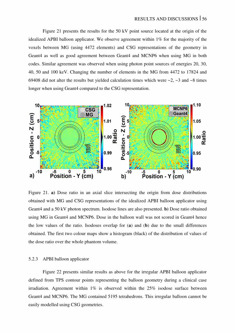
RESULTS AND DISCUSSIONS | 56
Figure 21 presents the results for the 50 kV point source located at the origin of the
idealized APBI balloon applicator. We observe agreement within 1% for the majority of the
voxels between MG (using 4472 elements) and CSG representations of the geometry in
Geant4 as well as good agreement between Geant4 and MCNP6 when using MG in both
codes. Similar agreement was observed when using photon point sources of energies 20, 30,
40, 50 and 100 keV. Changing the number of elements in the MG from 4472 to 17824 and
69408 did not alter the results but yielded calculation times which were ~2, ~3 and ~8 times
longer when using Geant4 compared to the CSG representation.
Figure 21. a) Dose ratio in an axial slice intersecting the origin from dose distributions
obtained with MG and CSG representations of the idealized APBI balloon applicator using
Geant4 and a 50 kV photon spectrum. Isodose lines are also presented. b) Dose ratio obtained
using MG in Geant4 and MCNP6. Dose in the balloon wall was not scored in Geant4 hence
the low values of the ratio. Isodoses overlap for (a) and (b) due to the small differences
obtained. The first two colour maps show a histogram (black) of the distribution of values of
the dose ratio over the whole phantom volume.
5.2.3 APBI balloon applicator
Figure 22 presents similar results as above for the irregular APBI balloon applicator
defined from TPS contour points representing the balloon geometry during a clinical case
irradiation. Agreement within 1% is observed within the 25% isodose surface between
Geant4 and MCNP6. The MG contained 5195 tetrahedrons. This irregular balloon cannot be
easily modelled using CSG geometries.

RESULTS AND DISCUSSIONS | 57
Figure 22. a) The MG of the irregular balloon. b) Axial plot of dose ratios obtained from
MCNP6 and Geant4 using the MG of the balloon and a 50 kV photon point source. Isodose
lines are also presented. Dose in the balloon wall was not scored in Geant4 hence the low
values of the ratio. The color map shows a histogram (extreme right) of the dose ratio
distribution over the whole phantom volume.
Figure 23. a) APBI balloon applicator wall represented by voxels. b) Axial dose ratio
obtained from MCNP6 using the voxel and MG models of the balloon.
Figure 23 shows a voxelized APBI balloon applicator slice and the dose ratio between
the results obtained with voxels and with MG. Differences of up to 30% were observed due
to the low geometric accuracy of the voxel model whose resolution exceeds the balloon
thickness by a factor of 2 and 5 for the voxel width/height and for the slice thickness,
respectively. Moreover, the balloon wall may be represented by more than one voxel
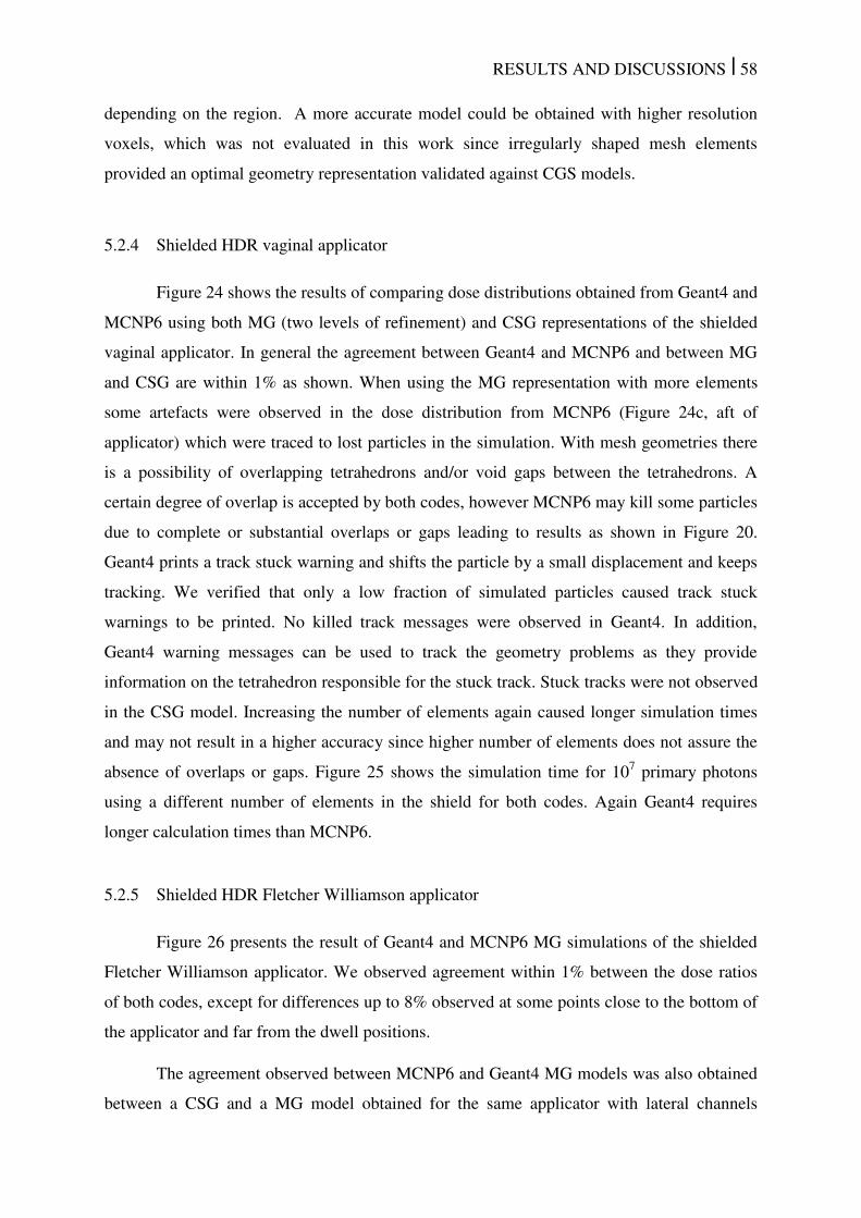
RESULTS AND DISCUSSIONS | 58
depending on the region. A more accurate model could be obtained with higher resolution
voxels, which was not evaluated in this work since irregularly shaped mesh elements
provided an optimal geometry representation validated against CGS models.
5.2.4 Shielded HDR vaginal applicator
Figure 24 shows the results of comparing dose distributions obtained from Geant4 and
MCNP6 using both MG (two levels of refinement) and CSG representations of the shielded
vaginal applicator. In general the agreement between Geant4 and MCNP6 and between MG
and CSG are within 1% as shown. When using the MG representation with more elements
some artefacts were observed in the dose distribution from MCNP6 (Figure 24c, aft of
applicator) which were traced to lost particles in the simulation. With mesh geometries there
is a possibility of overlapping tetrahedrons and/or void gaps between the tetrahedrons. A
certain degree of overlap is accepted by both codes, however MCNP6 may kill some particles
due to complete or substantial overlaps or gaps leading to results as shown in Figure 20.
Geant4 prints a track stuck warning and shifts the particle by a small displacement and keeps
tracking. We verified that only a low fraction of simulated particles caused track stuck
warnings to be printed. No killed track messages were observed in Geant4. In addition,
Geant4 warning messages can be used to track the geometry problems as they provide
information on the tetrahedron responsible for the stuck track. Stuck tracks were not observed
in the CSG model. Increasing the number of elements again caused longer simulation times
and may not result in a higher accuracy since higher number of elements does not assure the
absence of overlaps or gaps. Figure 25 shows the simulation time for 107 primary photons
using a different number of elements in the shield for both codes. Again Geant4 requires
longer calculation times than MCNP6.
5.2.5 Shielded HDR Fletcher Williamson applicator
Figure 26 presents the result of Geant4 and MCNP6 MG simulations of the shielded
Fletcher Williamson applicator. We observed agreement within 1% between the dose ratios
of both codes, except for differences up to 8% observed at some points close to the bottom of
the applicator and far from the dwell positions.
The agreement observed between MCNP6 and Geant4 MG models was also obtained
between a CSG and a MG model obtained for the same applicator with lateral channels
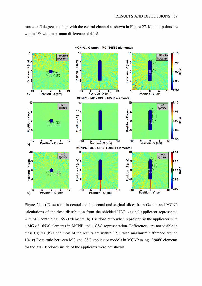
RESULTS AND DISCUSSIONS | 59
rotated 4.5 degrees to align with the central channel as shown in Figure 27. Most of points are
within 1% with maximum difference of 4.1%.
Figure 24. a) Dose ratio in central axial, coronal and sagittal slices from Geant4 and MCNP
calculations of the dose distribution from the shielded HDR vaginal applicator represented
with MG containing 16530 elements. b) The dose ratio when representing the applicator with
a MG of 16530 elements in MCNP and a CSG representation. Differences are not visible in
these figures (b) since most of the results are within 0.5% with maximum difference around
1%. c) Dose ratio between MG and CSG applicator models in MCNP using 129860 elements
for the MG. Isodoses inside of the applicator were not shown.
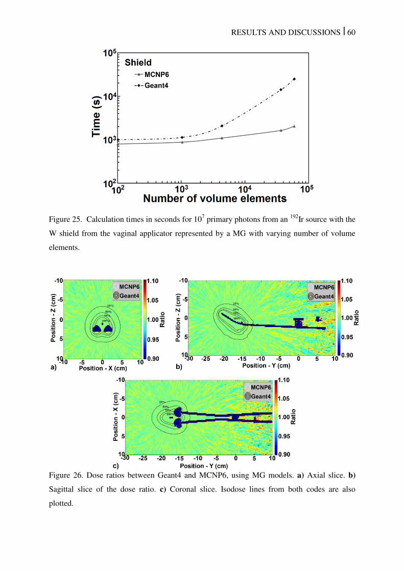
RESULTS AND DISCUSSIONS | 60
Figure 25. Calculation times in seconds for 107 primary photons from an
192Ir source with the
W shield from the vaginal applicator represented by a MG with varying number of volume
elements.
Figure 26. Dose ratios between Geant4 and MCNP6, using MG models. a) Axial slice. b)
Sagittal slice of the dose ratio. c) Coronal slice. Isodose lines from both codes are also
plotted.
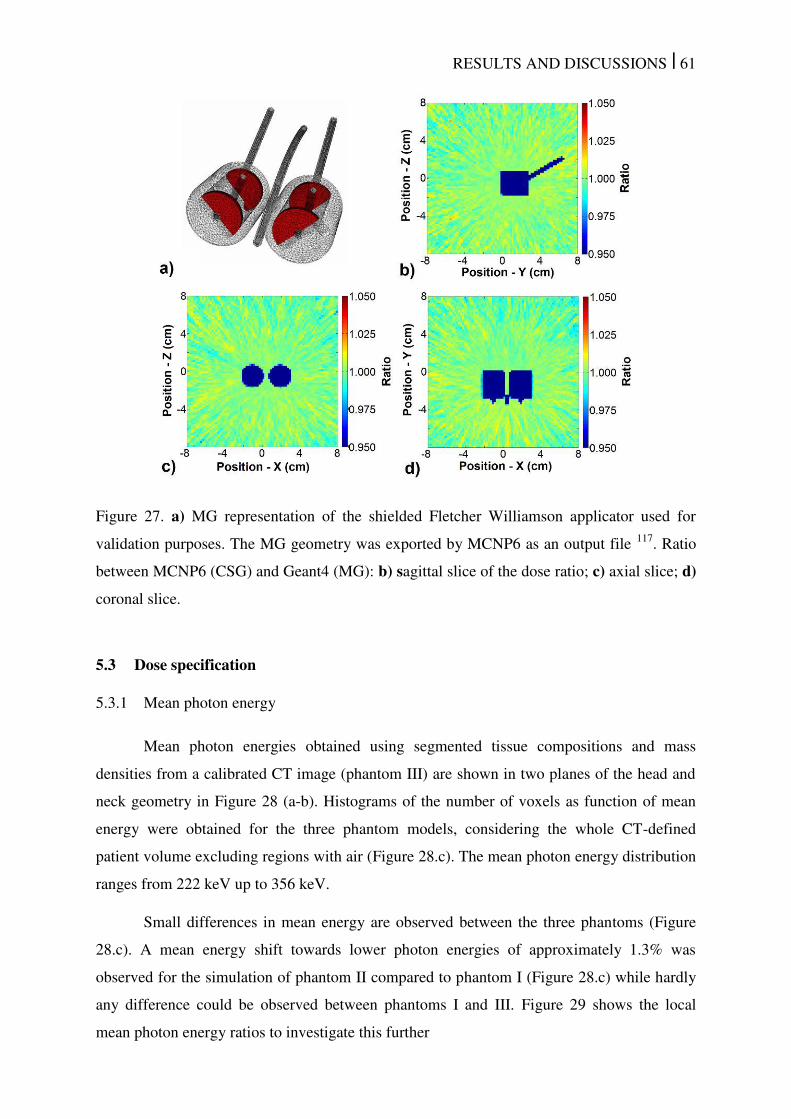
RESULTS AND DISCUSSIONS | 61
Figure 27. a) MG representation of the shielded Fletcher Williamson applicator used for
validation purposes. The MG geometry was exported by MCNP6 as an output file 117
. Ratio
between MCNP6 (CSG) and Geant4 (MG): b) sagittal slice of the dose ratio; c) axial slice; d)
coronal slice.
5.3 Dose specification
5.3.1 Mean photon energy
Mean photon energies obtained using segmented tissue compositions and mass
densities from a calibrated CT image (phantom III) are shown in two planes of the head and
neck geometry in Figure 28 (a-b). Histograms of the number of voxels as function of mean
energy were obtained for the three phantom models, considering the whole CT-defined
patient volume excluding regions with air (Figure 28.c). The mean photon energy distribution
ranges from 222 keV up to 356 keV.
Small differences in mean energy are observed between the three phantoms (Figure
28.c). A mean energy shift towards lower photon energies of approximately 1.3% was
observed for the simulation of phantom II compared to phantom I (Figure 28.c) while hardly
any difference could be observed between phantoms I and III. Figure 29 shows the local
mean photon energy ratios to investigate this further
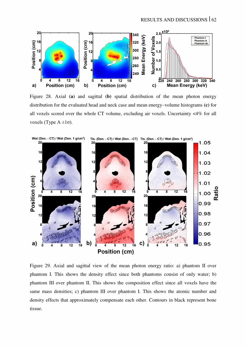
RESULTS AND DISCUSSIONS | 62
Figure 28. Axial (a) and sagittal (b) spatial distribution of the mean photon energy
distribution for the evaluated head and neck case and mean energy–volume histograms (c) for
all voxels scored over the whole CT volume, excluding air voxels. Uncertainty <4% for all
voxels (Type A ±1σ).
Figure 29. Axial and sagittal view of the mean photon energy ratio: a) phantom II over
phantom I. This shows the density effect since both phantoms consist of only water; b)
phantom III over phantom II. This shows the composition effect since all voxels have the
same mass densities; c) phantom III over phantom I. This shows the atomic number and
density effects that approximately compensate each other. Contours in black represent bone
tissue.
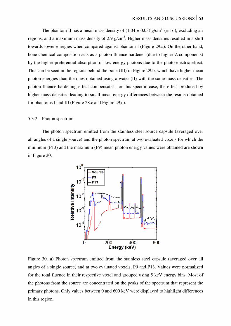
RESULTS AND DISCUSSIONS | 63
The phantom II has a mean mass density of (1.04 ± 0.03) g/cm3 (± 1σ), excluding air
regions, and a maximum mass density of 2.9 g/cm3. Higher mass densities resulted in a shift
towards lower energies when compared against phantom I (Figure 29.a). On the other hand,
bone chemical composition acts as a photon fluence hardener (due to higher Z components)
by the higher preferential absorption of low energy photons due to the photo-electric effect.
This can be seen in the regions behind the bone (III) in Figure 29.b, which have higher mean
photon energies than the ones obtained using a water (II) with the same mass densities. The
photon fluence hardening effect compensates, for this specific case, the effect produced by
higher mass densities leading to small mean energy differences between the results obtained
for phantoms I and III (Figure 28.c and Figure 29.c).
5.3.2 Photon spectrum
The photon spectrum emitted from the stainless steel source capsule (averaged over
all angles of a single source) and the photon spectrum at two evaluated voxels for which the
minimum (P13) and the maximum (P9) mean photon energy values were obtained are shown
in Figure 30.
Figure 30. a) Photon spectrum emitted from the stainless steel capsule (averaged over all
angles of a single source) and at two evaluated voxels, P9 and P13. Values were normalized
for the total fluence in their respective voxel and grouped using 5 keV energy bins. Most of
the photons from the source are concentrated on the peaks of the spectrum that represent the
primary photons. Only values between 0 and 600 keV were displayed to highlight differences
in this region.
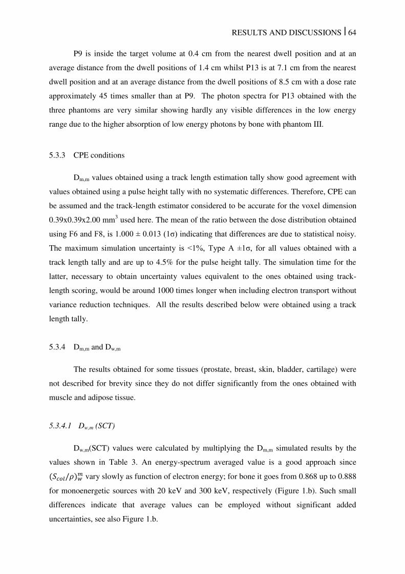
RESULTS AND DISCUSSIONS | 64
P9 is inside the target volume at 0.4 cm from the nearest dwell position and at an
average distance from the dwell positions of 1.4 cm whilst P13 is at 7.1 cm from the nearest
dwell position and at an average distance from the dwell positions of 8.5 cm with a dose rate
approximately 45 times smaller than at P9. The photon spectra for P13 obtained with the
three phantoms are very similar showing hardly any visible differences in the low energy
range due to the higher absorption of low energy photons by bone with phantom III.
5.3.3 CPE conditions
Dm,m values obtained using a track length estimation tally show good agreement with
values obtained using a pulse height tally with no systematic differences. Therefore, CPE can
be assumed and the track-length estimator considered to be accurate for the voxel dimension
0.39x0.39x2.00 mm3 used here. The mean of the ratio between the dose distribution obtained
using F6 and F8, is 1.000 ± 0.013 (1σ) indicating that differences are due to statistical noisy.
The maximum simulation uncertainty is <1%, Type A ±1σ, for all values obtained with a
track length tally and are up to 4.5% for the pulse height tally. The simulation time for the
latter, necessary to obtain uncertainty values equivalent to the ones obtained using track-
length scoring, would be around 1000 times longer when including electron transport without
variance reduction techniques. All the results described below were obtained using a track
length tally.
5.3.4 Dm,m and Dw,m
The results obtained for some tissues (prostate, breast, skin, bladder, cartilage) were
not described for brevity since they do not differ significantly from the ones obtained with
muscle and adipose tissue.
5.3.4.1 Dw,m (SCT)
Dw,m(SCT) values were calculated by multiplying the Dm,m simulated results by the
values shown in Table 3. An energy-spectrum averaged value is a good approach since /� � vary slowly as function of electron energy; for bone it goes from 0.868 up to 0.888
for monoenergetic sources with 20 keV and 300 keV, respectively (Figure 1.b). Such small
differences indicate that average values can be employed without significant added
uncertainties, see also Figure 1.b.
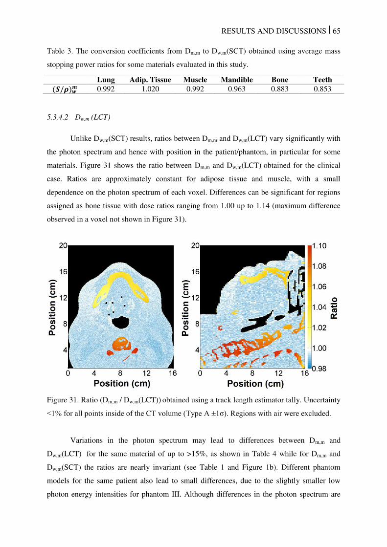
RESULTS AND DISCUSSIONS | 65
Table 3. The conversion coefficients from Dm,m to Dw,m(SCT) obtained using average mass
stopping power ratios for some materials evaluated in this study.
5.3.4.2 Dw,m (LCT)
Unlike Dw,m(SCT) results, ratios between Dm,m and Dw,m(LCT) vary significantly with
the photon spectrum and hence with position in the patient/phantom, in particular for some
materials. Figure 31 shows the ratio between Dm,m and Dw,m(LCT) obtained for the clinical
case. Ratios are approximately constant for adipose tissue and muscle, with a small
dependence on the photon spectrum of each voxel. Differences can be significant for regions
assigned as bone tissue with dose ratios ranging from 1.00 up to 1.14 (maximum difference
observed in a voxel not shown in Figure 31).
Figure 31. Ratio (Dm,m / Dw,m(LCT)) obtained using a track length estimator tally. Uncertainty
<1% for all points inside of the CT volume (Type A ±1σ). Regions with air were excluded.
Variations in the photon spectrum may lead to differences between Dm,m and
Dw,m(LCT) for the same material of up to >15%, as shown in Table 4 while for Dm,m and
Dw,m(SCT) the ratios are nearly invariant (see Table 1 and Figure 1b). Different phantom
models for the same patient also lead to small differences, due to the slightly smaller low
photon energy intensities for phantom III. Although differences in the photon spectrum are
Lung Adip. Tissue Muscle Mandible Bone Teeth �/� � 0.992 1.020 0.992 0.963 0.883 0.853
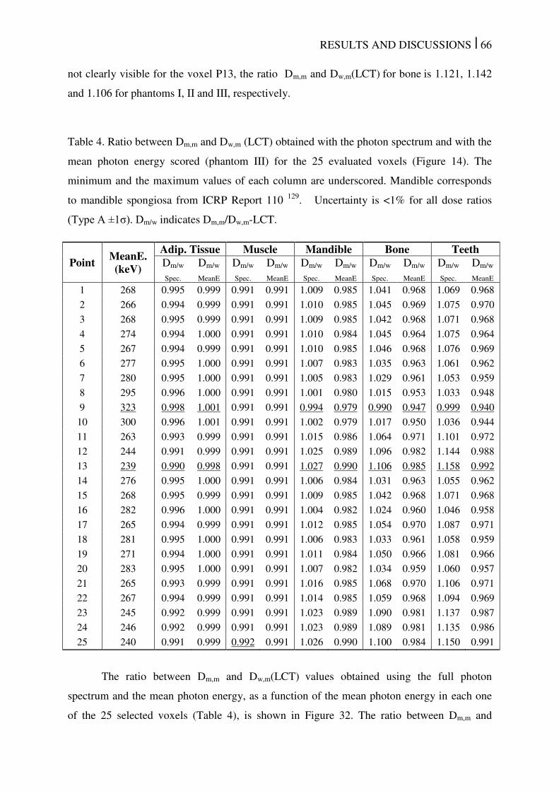
RESULTS AND DISCUSSIONS | 66
not clearly visible for the voxel P13, the ratio Dm,m and Dw,m(LCT) for bone is 1.121, 1.142
and 1.106 for phantoms I, II and III, respectively.
Table 4. Ratio between Dm,m and Dw,m (LCT) obtained with the photon spectrum and with the
mean photon energy scored (phantom III) for the 25 evaluated voxels (Figure 14). The
minimum and the maximum values of each column are underscored. Mandible corresponds
to mandible spongiosa from ICRP Report 110 129
. Uncertainty is <1% for all dose ratios
(Type A ±1σ). Dm/w indicates Dm,m/Dw,m-LCT.
Point MeanE. (keV)
Adip. Tissue Muscle Mandible Bone Teeth Dm/w
Spec.
Dm/w
MeanE
Dm/w
Spec.
Dm/w
MeanE
Dm/w
Spec.
Dm/w
MeanE
Dm/w
Spec.
Dm/w
MeanE
Dm/w
Spec.
Dm/w
MeanE
1 268 0.995 0.999 0.991 0.991 1.009 0.985 1.041 0.968 1.069 0.968
2 266 0.994 0.999 0.991 0.991 1.010 0.985 1.045 0.969 1.075 0.970
3 268 0.995 0.999 0.991 0.991 1.009 0.985 1.042 0.968 1.071 0.968
4 274 0.994 1.000 0.991 0.991 1.010 0.984 1.045 0.964 1.075 0.964
5 267 0.994 0.999 0.991 0.991 1.010 0.985 1.046 0.968 1.076 0.969
6 277 0.995 1.000 0.991 0.991 1.007 0.983 1.035 0.963 1.061 0.962
7 280 0.995 1.000 0.991 0.991 1.005 0.983 1.029 0.961 1.053 0.959
8 295 0.996 1.000 0.991 0.991 1.001 0.980 1.015 0.953 1.033 0.948
9 323 0.998 1.001 0.991 0.991 0.994 0.979 0.990 0.947 0.999 0.940
10 300 0.996 1.001 0.991 0.991 1.002 0.979 1.017 0.950 1.036 0.944
11 263 0.993 0.999 0.991 0.991 1.015 0.986 1.064 0.971 1.101 0.972
12 244 0.991 0.999 0.991 0.991 1.025 0.989 1.096 0.982 1.144 0.988
13 239 0.990 0.998 0.991 0.991 1.027 0.990 1.106 0.985 1.158 0.992
14 276 0.995 1.000 0.991 0.991 1.006 0.984 1.031 0.963 1.055 0.962
15 268 0.995 0.999 0.991 0.991 1.009 0.985 1.042 0.968 1.071 0.968
16 282 0.996 1.000 0.991 0.991 1.004 0.982 1.024 0.960 1.046 0.958
17 265 0.994 0.999 0.991 0.991 1.012 0.985 1.054 0.970 1.087 0.971
18 281 0.995 1.000 0.991 0.991 1.006 0.983 1.033 0.961 1.058 0.959
19 271 0.994 1.000 0.991 0.991 1.011 0.984 1.050 0.966 1.081 0.966
20 283 0.995 1.000 0.991 0.991 1.007 0.982 1.034 0.959 1.060 0.957
21 265 0.993 0.999 0.991 0.991 1.016 0.985 1.068 0.970 1.106 0.971
22 267 0.994 0.999 0.991 0.991 1.014 0.985 1.059 0.968 1.094 0.969
23 245 0.992 0.999 0.991 0.991 1.023 0.989 1.090 0.981 1.137 0.987
24 246 0.992 0.999 0.991 0.991 1.023 0.989 1.089 0.981 1.135 0.986
25 240 0.991 0.999 0.992 0.991 1.026 0.990 1.100 0.984 1.150 0.991
The ratio between Dm,m and Dw,m(LCT) values obtained using the full photon
spectrum and the mean photon energy, as a function of the mean photon energy in each one
of the 25 selected voxels (Table 4), is shown in Figure 32. The ratio between Dm,m and
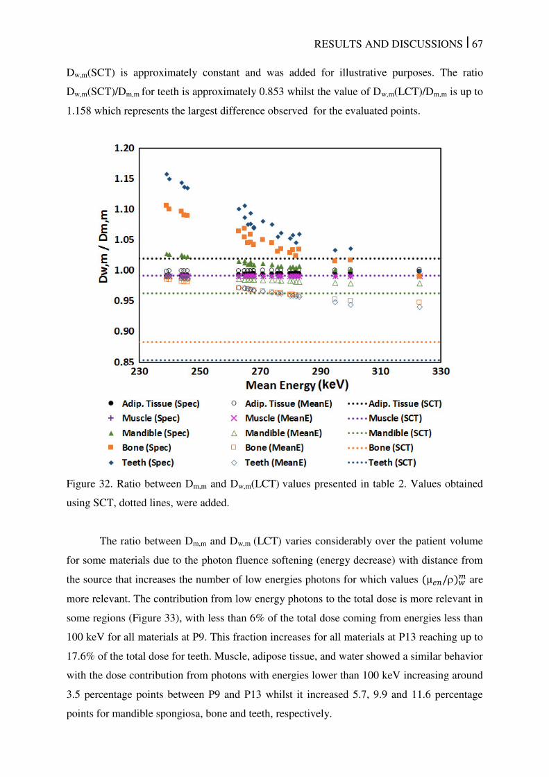
RESULTS AND DISCUSSIONS | 67
Dw,m(SCT) is approximately constant and was added for illustrative purposes. The ratio
Dw,m(SCT)/Dm,m for teeth is approximately 0.853 whilst the value of Dw,m(LCT)/Dm,m is up to
1.158 which represents the largest difference observed for the evaluated points.
Figure 32. Ratio between Dm,m and Dw,m(LCT) values presented in table 2. Values obtained
using SCT, dotted lines, were added.
The ratio between Dm,m and Dw,m (LCT) varies considerably over the patient volume
for some materials due to the photon fluence softening (energy decrease) with distance from
the source that increases the number of low energies photons for which values µ / � are
more relevant. The contribution from low energy photons to the total dose is more relevant in
some regions (Figure 33), with less than 6% of the total dose coming from energies less than
100 keV for all materials at P9. This fraction increases for all materials at P13 reaching up to
17.6% of the total dose for teeth. Muscle, adipose tissue, and water showed a similar behavior
with the dose contribution from photons with energies lower than 100 keV increasing around
3.5 percentage points between P9 and P13 whilst it increased 5.7, 9.9 and 11.6 percentage
points for mandible spongiosa, bone and teeth, respectively.
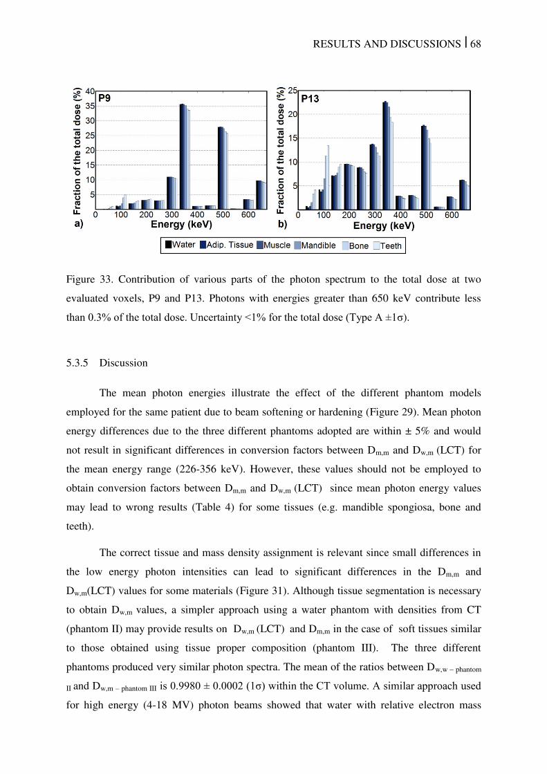
RESULTS AND DISCUSSIONS | 68
Figure 33. Contribution of various parts of the photon spectrum to the total dose at two
evaluated voxels, P9 and P13. Photons with energies greater than 650 keV contribute less
than 0.3% of the total dose. Uncertainty <1% for the total dose (Type A ±1σ).
5.3.5 Discussion
The mean photon energies illustrate the effect of the different phantom models
employed for the same patient due to beam softening or hardening (Figure 29). Mean photon
energy differences due to the three different phantoms adopted are within ± 5% and would
not result in significant differences in conversion factors between Dm,m and Dw,m (LCT) for
the mean energy range (226-356 keV). However, these values should not be employed to
obtain conversion factors between Dm,m and Dw,m (LCT) since mean photon energy values
may lead to wrong results (Table 4) for some tissues (e.g. mandible spongiosa, bone and
teeth).
The correct tissue and mass density assignment is relevant since small differences in
the low energy photon intensities can lead to significant differences in the Dm,m and
Dw,m(LCT) values for some materials (Figure 31). Although tissue segmentation is necessary
to obtain Dw,m values, a simpler approach using a water phantom with densities from CT
(phantom II) may provide results on Dw,m (LCT) and Dm,m in the case of soft tissues similar
to those obtained using tissue proper composition (phantom III). The three different
phantoms produced very similar photon spectra. The mean of the ratios between Dw,w – phantom
II and Dw,m – phantom III is 0.9980 ± 0.0002 (1σ) within the CT volume. A similar approach used
for high energy (4-18 MV) photon beams showed that water with relative electron mass
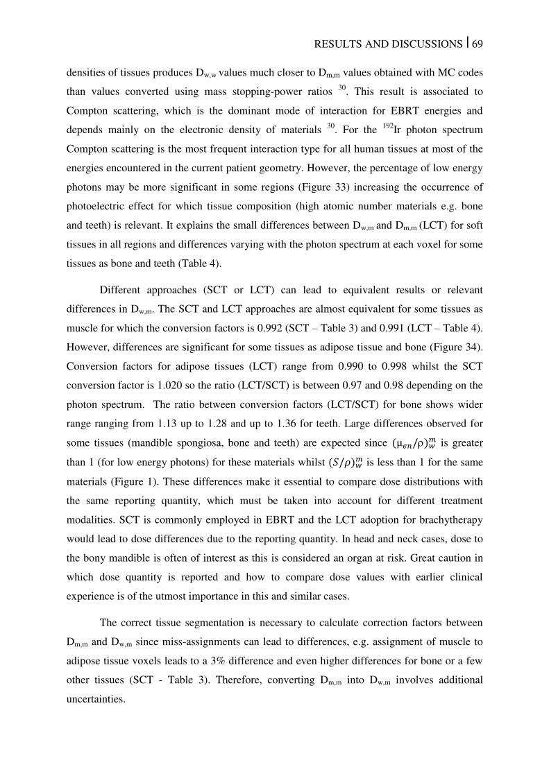
RESULTS AND DISCUSSIONS | 69
densities of tissues produces Dw,w values much closer to Dm,m values obtained with MC codes
than values converted using mass stopping-power ratios 30
. This result is associated to
Compton scattering, which is the dominant mode of interaction for EBRT energies and
depends mainly on the electronic density of materials 30
. For the 192
Ir photon spectrum
Compton scattering is the most frequent interaction type for all human tissues at most of the
energies encountered in the current patient geometry. However, the percentage of low energy
photons may be more significant in some regions (Figure 33) increasing the occurrence of
photoelectric effect for which tissue composition (high atomic number materials e.g. bone
and teeth) is relevant. It explains the small differences between Dw,m and Dm,m (LCT) for soft
tissues in all regions and differences varying with the photon spectrum at each voxel for some
tissues as bone and teeth (Table 4).
Different approaches (SCT or LCT) can lead to equivalent results or relevant
differences in Dw,m. The SCT and LCT approaches are almost equivalent for some tissues as
muscle for which the conversion factors is 0.992 (SCT – Table 3) and 0.991 (LCT – Table 4).
However, differences are significant for some tissues as adipose tissue and bone (Figure 34).
Conversion factors for adipose tissues (LCT) range from 0.990 to 0.998 whilst the SCT
conversion factor is 1.020 so the ratio (LCT/SCT) is between 0.97 and 0.98 depending on the
photon spectrum. The ratio between conversion factors (LCT/SCT) for bone shows wider
range ranging from 1.13 up to 1.28 and up to 1.36 for teeth. Large differences observed for
some tissues (mandible spongiosa, bone and teeth) are expected since µ / � is greater
than 1 (for low energy photons) for these materials whilst /� � is less than 1 for the same
materials (Figure 1). These differences make it essential to compare dose distributions with
the same reporting quantity, which must be taken into account for different treatment
modalities. SCT is commonly employed in EBRT and the LCT adoption for brachytherapy
would lead to dose differences due to the reporting quantity. In head and neck cases, dose to
the bony mandible is often of interest as this is considered an organ at risk. Great caution in
which dose quantity is reported and how to compare dose values with earlier clinical
experience is of the utmost importance in this and similar cases.
The correct tissue segmentation is necessary to calculate correction factors between
Dm,m and Dw,m since miss-assignments can lead to differences, e.g. assignment of muscle to
adipose tissue voxels leads to a 3% difference and even higher differences for bone or a few
other tissues (SCT - Table 3). Therefore, converting Dm,m into Dw,m involves additional
uncertainties.
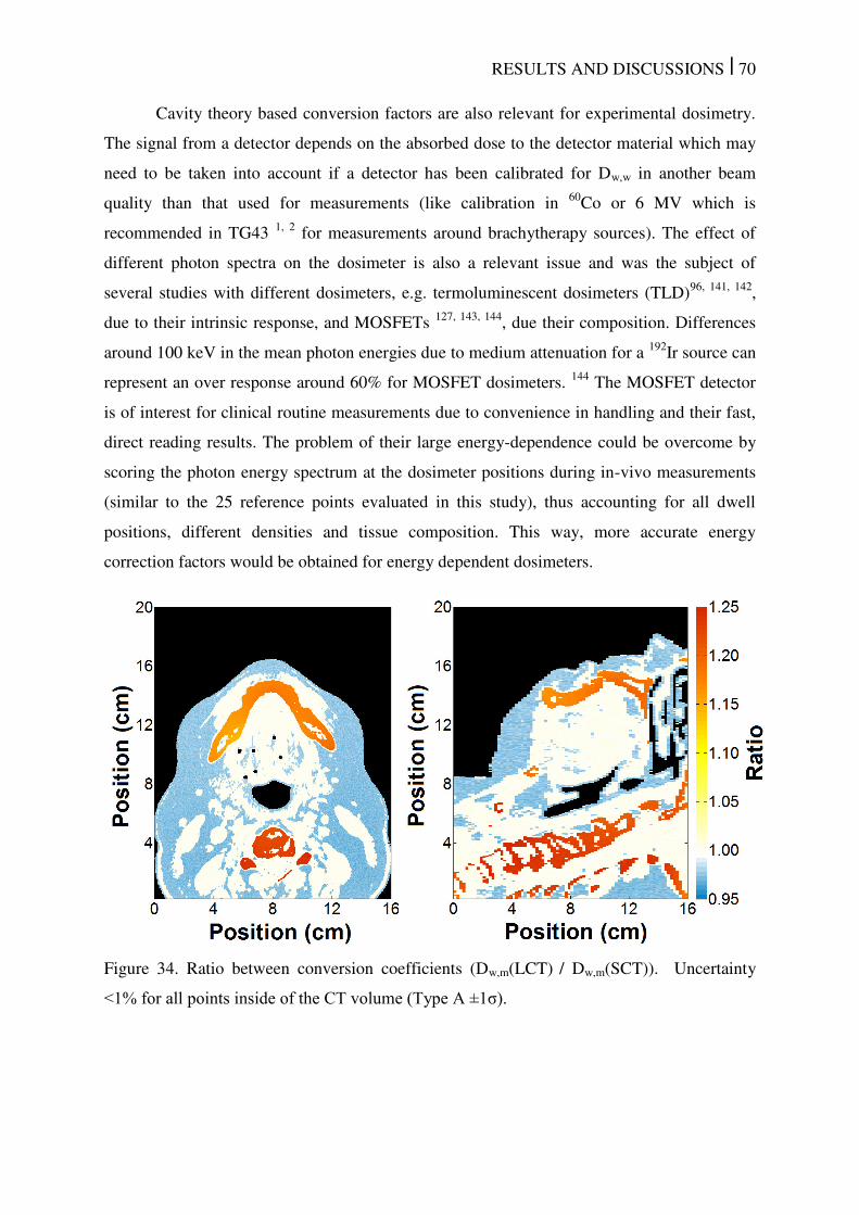
RESULTS AND DISCUSSIONS | 70
Cavity theory based conversion factors are also relevant for experimental dosimetry.
The signal from a detector depends on the absorbed dose to the detector material which may
need to be taken into account if a detector has been calibrated for Dw,w in another beam
quality than that used for measurements (like calibration in 60
Co or 6 MV which is
recommended in TG43 1, 2
for measurements around brachytherapy sources). The effect of
different photon spectra on the dosimeter is also a relevant issue and was the subject of
several studies with different dosimeters, e.g. termoluminescent dosimeters (TLD)96, 141, 142
,
due to their intrinsic response, and MOSFETs 127, 143, 144
, due their composition. Differences
around 100 keV in the mean photon energies due to medium attenuation for a 192
Ir source can
represent an over response around 60% for MOSFET dosimeters. 144
The MOSFET detector
is of interest for clinical routine measurements due to convenience in handling and their fast,
direct reading results. The problem of their large energy-dependence could be overcome by
scoring the photon energy spectrum at the dosimeter positions during in-vivo measurements
(similar to the 25 reference points evaluated in this study), thus accounting for all dwell
positions, different densities and tissue composition. This way, more accurate energy
correction factors would be obtained for energy dependent dosimeters.
Figure 34. Ratio between conversion coefficients (Dw,m(LCT) / Dw,m(SCT)). Uncertainty
<1% for all points inside of the CT volume (Type A ±1σ).
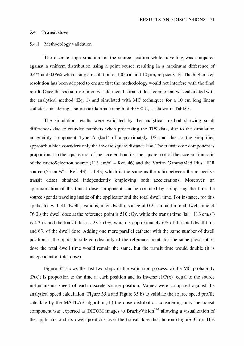
RESULTS AND DISCUSSIONS | 71
5.4 Transit dose
5.4.1 Methodology validation
The discrete approximation for the source position while travelling was compared
against a uniform distribution using a point source resulting in a maximum difference of
0.6% and 0.06% when using a resolution of 100 µm and 10 µm, respectively. The higher step
resolution has been adopted to ensure that the methodology would not interfere with the final
result. Once the spatial resolution was defined the transit dose component was calculated with
the analytical method (Eq. 1) and simulated with MC techniques for a 10 cm long linear
catheter considering a source air-kerma strength of 40700 U, as shown in Table 5.
The simulation results were validated by the analytical method showing small
differences due to rounded numbers when processing the TPS data, due to the simulation
uncertainty component Type A (k=1) of approximately 1% and due to the simplified
approach which considers only the inverse square distance law. The transit dose component is
proportional to the square root of the acceleration, i.e. the square root of the acceleration ratio
of the microSelectron source (113 cm/s2 – Ref. 46)
and the Varian GammaMed Plus HDR
source (55 cm/s2 – Ref. 43) is 1.43, which is the same as the ratio between the respective
transit doses obtained independently employing both accelerations. Moreover, an
approximation of the transit dose component can be obtained by comparing the time the
source spends traveling inside of the applicator and the total dwell time. For instance, for this
applicator with 41 dwell positions, inter-dwell distance of 0.25 cm and a total dwell time of
76.0 s the dwell dose at the reference point is 510 cGy, while the transit time (|a| = 113 cm/s2)
is 4.25 s and the transit dose is 28.5 cGy, which is approximately 6% of the total dwell time
and 6% of the dwell dose. Adding one more parallel catheter with the same number of dwell
position at the opposite side equidistantly of the reference point, for the same prescription
dose the total dwell time would remain the same, but the transit time would double (it is
independent of total dose).
Figure 35 shows the last two steps of the validation process: a) the MC probability
(P(x)) is proportion to the time at each position and its inverse (1/P(x)) equal to the source
instantaneous speed of each discrete source position. Values were compared against the
analytical speed calculation (Figure 35.a and Figure 35.b) to validate the source speed profile
calculate by the MATLAB algorithm; b) the dose distribution considering only the transit
component was exported as DICOM images to BrachyVisionTM
allowing a visualization of
the applicator and its dwell positions over the transit dose distribution (Figure 35.c). This

RESULTS AND DISCUSSIONS | 72
figure shows that the transit dose distribution for a uniform accelerated movement follows the
applicator geometry and has a higher dose deposition near the dwell positions, due to the
source slowing down.
Table 5. Transit dose for a reference point orthogonal to the catheter’s longitudinal axis and
positioned at 0.5 cm from its center (Figure 15.a). The values were calculated analytically
(An) and simulated (MC) extracting the information from a treatment plan created with
BrachyVisionTM
. The underlined speeds were obtained considering a uniform accelerated
movement for an acceleration of 113 cm/s2 (Nucletron
46) and 55 cm/s
2 (Varian
43).
Inter-dwell distance (cm) 0.25 0.5 1 2
(cm/s)
Dose (cGy) (cm/s)
Dose (cGy) (cm/s)
Dose (cGy) (cm/s)
Dose (cGy) An. MC An. MC An. MC An. MC
60.0 2.5 2.5 60.0 2.5 2.5 60.0 2.5 2.5 60.0 2.5 2.5
30.0 5.0 5.0 30.0 5.0 5.0 30.0 5.0 5.0 30.0 5.0 5.0
*2.7 30.5 30.5 3.8 22.5 22.5 5.3 17.0 17.0 7.5 12.9 12.9
2.7 30.1 30.0 3.8 22.0 22.1 5.3 16.7 16.6 7.5 10.7 10.6
**2.2 38.0 38.5 3.1 28.3 28.3 4.4 21.2 21.2 6.2 16.4 16.4
2.2 43.1 43.0 3.1 31.5 31.6 4.4 23.9 23.9 6.2 15.3 15.2
*values obtained with an average return speed of 23.8 cm/s.
**values obtained with an average return speed of 16.6 cm/s.
Figure 35. a) Source instantaneous speed, derived from the source trajectory and dwell
positions, for each discrete source position compared against analytical calculation for the
source approaching the first dwell position at 5 cm and moving between the dwell positions
(right to left) up to the last dwell position that was defined as the origin; b) instantaneous
speed validation for the source coming back to the safe; c) BrachyVisionTM
ring applicator
showing the dwell positions (black boxes) superimposed over a transit dose distribution
without the dwell dose component.
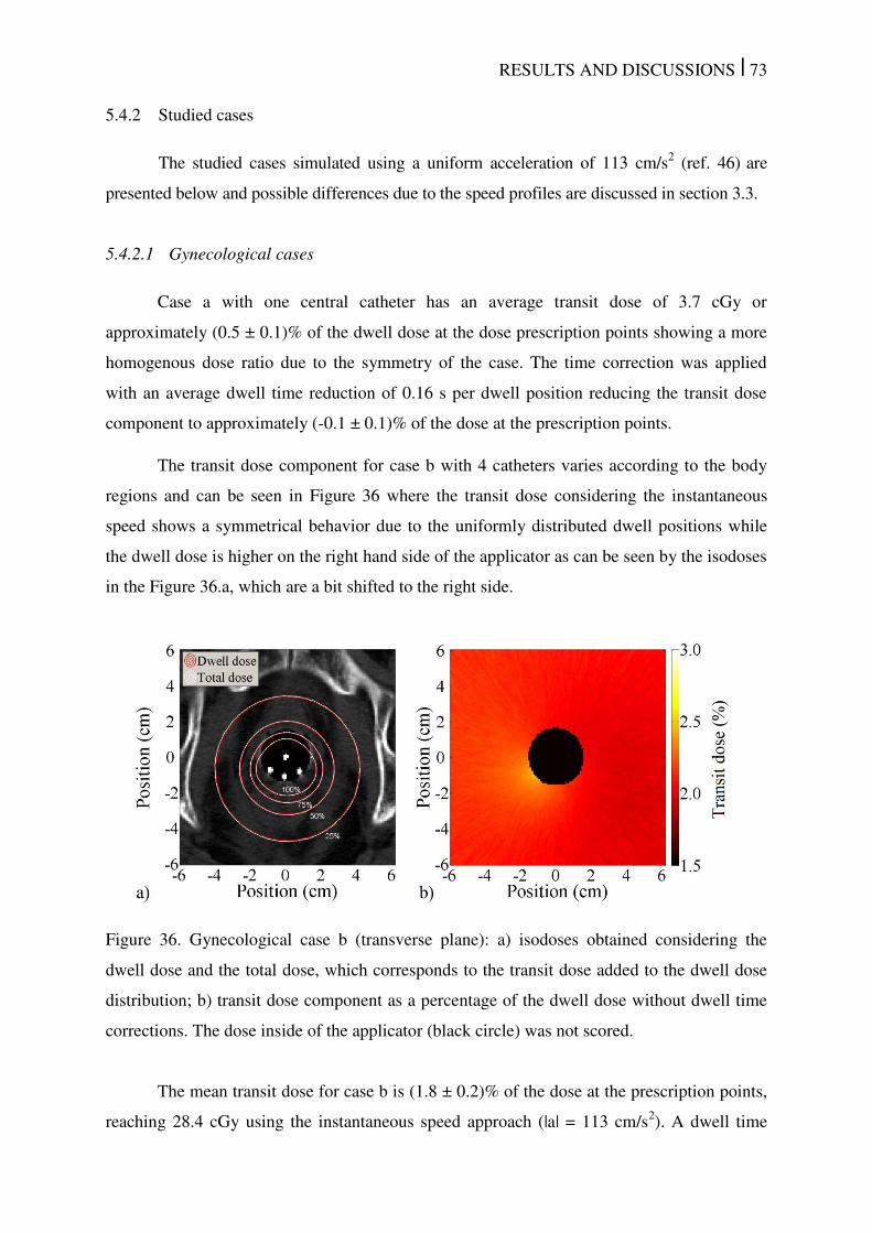
RESULTS AND DISCUSSIONS | 73
5.4.2 Studied cases
The studied cases simulated using a uniform acceleration of 113 cm/s2 (ref. 46)
are
presented below and possible differences due to the speed profiles are discussed in section 3.3.
5.4.2.1 Gynecological cases
Case a with one central catheter has an average transit dose of 3.7 cGy or
approximately (0.5 ± 0.1)% of the dwell dose at the dose prescription points showing a more
homogenous dose ratio due to the symmetry of the case. The time correction was applied
with an average dwell time reduction of 0.16 s per dwell position reducing the transit dose
component to approximately (-0.1 ± 0.1)% of the dose at the prescription points.
The transit dose component for case b with 4 catheters varies according to the body
regions and can be seen in Figure 36 where the transit dose considering the instantaneous
speed shows a symmetrical behavior due to the uniformly distributed dwell positions while
the dwell dose is higher on the right hand side of the applicator as can be seen by the isodoses
in the Figure 36.a, which are a bit shifted to the right side.
Figure 36. Gynecological case b (transverse plane): a) isodoses obtained considering the
dwell dose and the total dose, which corresponds to the transit dose added to the dwell dose
distribution; b) transit dose component as a percentage of the dwell dose without dwell time
corrections. The dose inside of the applicator (black circle) was not scored.
The mean transit dose for case b is (1.8 ± 0.2)% of the dose at the prescription points,
reaching 28.4 cGy using the instantaneous speed approach (|a| = 113 cm/s2). A dwell time
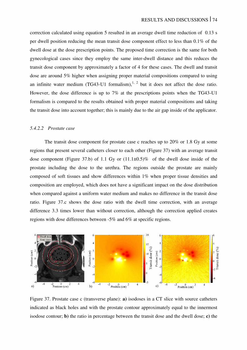
RESULTS AND DISCUSSIONS | 74
correction calculated using equation 5 resulted in an average dwell time reduction of 0.13 s
per dwell position reducing the mean transit dose component effect to less than 0.1% of the
dwell dose at the dose prescription points. The proposed time correction is the same for both
gynecological cases since they employ the same inter-dwell distance and this reduces the
transit dose component by approximately a factor of 4 for these cases. The dwell and transit
dose are around 5% higher when assigning proper material compositions compared to using
an infinite water medium (TG43-U1 formalism),1, 2
but it does not affect the dose ratio.
However, the dose difference is up to 7% at the prescriptions points when the TG43-U1
formalism is compared to the results obtained with proper material compositions and taking
the transit dose into account together; this is mainly due to the air gap inside of the applicator.
5.4.2.2 Prostate case
The transit dose component for prostate case c reaches up to 20% or 1.8 Gy at some
regions that present several catheters closer to each other (Figure 37) with an average transit
dose component (Figure 37.b) of 1.1 Gy or (11.1±0.5)% of the dwell dose inside of the
prostate including the dose to the urethra. The regions outside the prostate are mainly
composed of soft tissues and show differences within 1% when proper tissue densities and
composition are employed, which does not have a significant impact on the dose distribution
when compared against a uniform water medium and makes no difference in the transit dose
ratio. Figure 37.c shows the dose ratio with the dwell time correction, with an average
difference 3.3 times lower than without correction, although the correction applied creates
regions with dose differences between -5% and 6% at specific regions.
Figure 37. Prostate case c (transverse plane): a) isodoses in a CT slice with source catheters
indicated as black holes and with the prostate contour approximately equal to the innermost
isodose contour; b) the ratio in percentage between the transit dose and the dwell dose; c) the
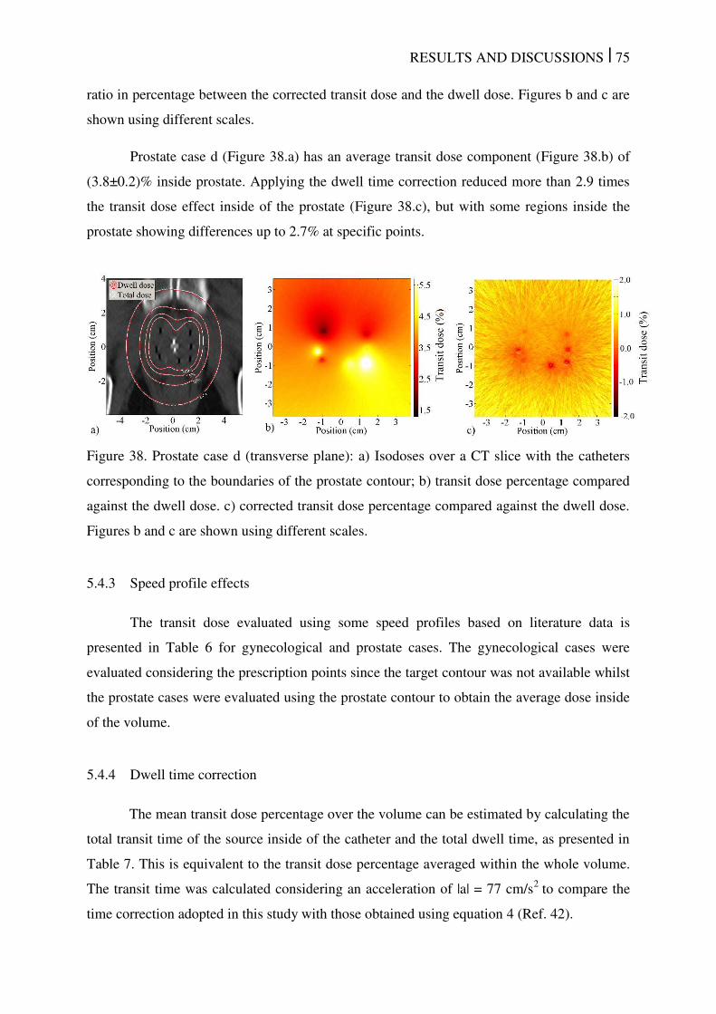
RESULTS AND DISCUSSIONS | 75
ratio in percentage between the corrected transit dose and the dwell dose. Figures b and c are
shown using different scales.
Prostate case d (Figure 38.a) has an average transit dose component (Figure 38.b) of
(3.8±0.2)% inside prostate. Applying the dwell time correction reduced more than 2.9 times
the transit dose effect inside of the prostate (Figure 38.c), but with some regions inside the
prostate showing differences up to 2.7% at specific points.
Figure 38. Prostate case d (transverse plane): a) Isodoses over a CT slice with the catheters
corresponding to the boundaries of the prostate contour; b) transit dose percentage compared
against the dwell dose. c) corrected transit dose percentage compared against the dwell dose.
Figures b and c are shown using different scales.
5.4.3 Speed profile effects
The transit dose evaluated using some speed profiles based on literature data is
presented in Table 6 for gynecological and prostate cases. The gynecological cases were
evaluated considering the prescription points since the target contour was not available whilst
the prostate cases were evaluated using the prostate contour to obtain the average dose inside
of the volume.
5.4.4 Dwell time correction
The mean transit dose percentage over the volume can be estimated by calculating the
total transit time of the source inside of the catheter and the total dwell time, as presented in
Table 7. This is equivalent to the transit dose percentage averaged within the whole volume.
The transit time was calculated considering an acceleration of |a| = 77 cm/s2
to compare the
time correction adopted in this study with those obtained using equation 4 (Ref. 42).
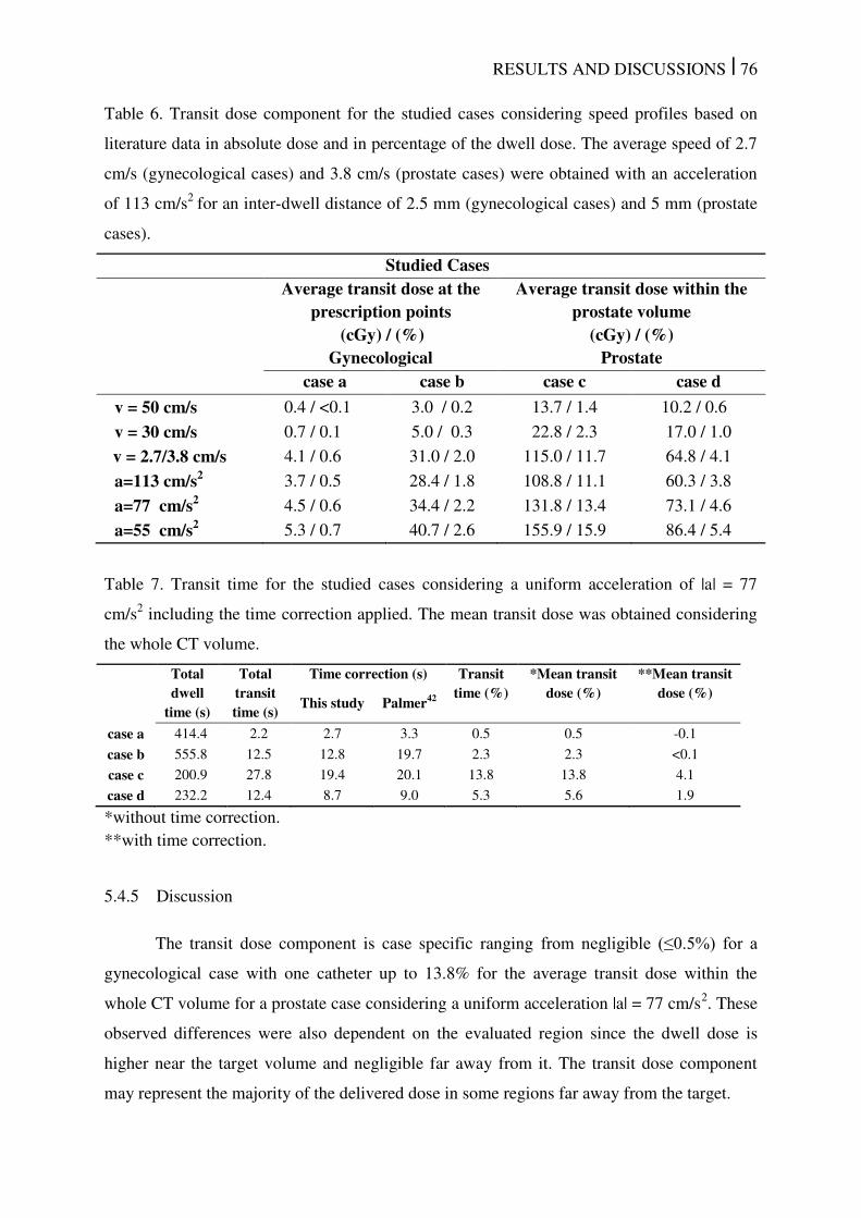
RESULTS AND DISCUSSIONS | 76
Table 6. Transit dose component for the studied cases considering speed profiles based on
literature data in absolute dose and in percentage of the dwell dose. The average speed of 2.7
cm/s (gynecological cases) and 3.8 cm/s (prostate cases) were obtained with an acceleration
of 113 cm/s2
for an inter-dwell distance of 2.5 mm (gynecological cases) and 5 mm (prostate
cases).
Studied Cases Average transit dose at the
prescription points (cGy) / (%)
Average transit dose within the prostate volume
(cGy) / (%) Gynecological Prostate case a case b case c case d
v = 50 cm/s 0.4 / <0.1 3.0 / 0.2 13.7 / 1.4 10.2 / 0.6
v = 30 cm/s 0.7 / 0.1 5.0 / 0.3 22.8 / 2.3 17.0 / 1.0
v = 2.7/3.8 cm/s 4.1 / 0.6 31.0 / 2.0 115.0 / 11.7 64.8 / 4.1
a=113 cm/s2 3.7 / 0.5 28.4 / 1.8 108.8 / 11.1 60.3 / 3.8
a=77 cm/s2 4.5 / 0.6 34.4 / 2.2 131.8 / 13.4 73.1 / 4.6
a=55 cm/s2 5.3 / 0.7 40.7 / 2.6 155.9 / 15.9 86.4 / 5.4
Table 7. Transit time for the studied cases considering a uniform acceleration of |a| = 77
cm/s2 including the time correction applied. The mean transit dose was obtained considering
the whole CT volume.
Total dwell
time (s)
Total transit time (s)
Time correction (s) Transit time (%)
*Mean transit dose (%)
**Mean transit dose (%)
This study Palmer42
case a 414.4 2.2 2.7 3.3 0.5 0.5 -0.1
case b 555.8 12.5 12.8 19.7 2.3 2.3 <0.1
case c 200.9 27.8 19.4 20.1 13.8 13.8 4.1
case d 232.2 12.4 8.7 9.0 5.3 5.6 1.9
*without time correction.
**with time correction.
5.4.5 Discussion
The transit dose component is case specific ranging from negligible (≤0.5%) for a
gynecological case with one catheter up to 13.8% for the average transit dose within the
whole CT volume for a prostate case considering a uniform acceleration |a| = 77 cm/s2. These
observed differences were also dependent on the evaluated region since the dwell dose is
higher near the target volume and negligible far away from it. The transit dose component
may represent the majority of the delivered dose in some regions far away from the target.
RESULTS AND DISCUSSIONS | 77
The gynecological case with one catheter employed prescription points at 0.5 cm from
the surface of the applicator which is 2.25 cm away from the dwell positions resulting in long
dwell times which leads to a negligible transit dose component relative to the dwell dose.
However, the transit component may not be negligible for other similar cases. For instance,
the transit component for the gynecological case with four catheters is approximately 4 times
higher than the first case due to the number of catheters. Even larger differences were
observed between the intracavitary and the interstitial prostate cases since the latter modality
has much lower dwell times than the gynecological cases due to the proximity of the treated
region. Moreover, the evaluated prostate cases use several catheters (up to 16) which, in
general, results in longer travel times leading to a more significant transit dose component.
Significant dose differences were also observed between the interstitial cases. The
prostate case d was performed using a more uniform catheter and dwell position distribution
inside the prostate and with less than half the number of catheters and dwell positions than in
case c. Due to these differences the transit dose component inside the prostate volume in case
d is approximately 3 times lower than in case c. Differences between the cases can be easily
visualized by comparing the source travel time and the total dwell time presented in Table 7,
which also provides an estimative of the average transit dose.
Although an estimative of the average transit dose can be obtained using the
relationship between travel and dwell times, a uniform acceleration results in transit dose hot
spots near the dwell positions and lower transit doses in between them leading to a complex
transit dose distribution. This complexity level depends on the speed profile, number of
catheters, dwell positions and their spatial distribution. These factors associated with a
limited number of dwell positions do not allow a full transit dose compensation just by
reducing the dwell time. This approach may lead to cold and hot spots since the time
correction necessary to reduce the transit dose near the dwell positions may result in an
underdose in other regions. Nevertheless, the applied dwell time corrections reduced
considerably the transit dose component for our cases and produced more homogeneous
distributions when using an accurate speed profile (Figure 37).
Tenfold differences can be observed between the speed scenario for the
microSelectron (an average speed of 50 cm/s) and the worst scenario (uniform acceleration of
|a| = 55 cm/s2) for all cases. The average transit dose inside the prostate volume obtained
using an average or instantaneous variable speed with the same acceleration value were
equivalent. However, these approaches lead to different transit dose distributions since the
RESULTS AND DISCUSSIONS | 78
transit dose near the dwell positions is much higher using the latter approach due to the
source slowing down near the dwell positions.
The source travel time between the dwell positions is the main component of the
transit dose within the target volume, which was the main interest in this study. However,
when the acceleration is assumed uniform for the transit dose calculation a maximum source
speed should be defined, otherwise the source could attain unrealistic speeds when exiting
from the safe or returning to it. This study used 52 cm/s as the maximum source speed;
different speed values showed no significant difference for the transit dose component for the
studied cases due to the assumed trajectory length. These trajectories imported from the
treatment plan have limited lengths since they cover mainly the region with dwell positions
due to its clinical relevance. The source, in general, does not reach its maximum speed close
to the target; this happens only over a few centimeters far away from the target volume.
5.5 Speed measurements
Figure 39.a shows the average speed ( . ) for the average of 6 measurements,
consisting of 3 arrival profiles and 3 return profiles. Video 1 shows an example of the
measurements with one dwell position at the end of the trajectory. There is no continuous
slowing down since the motor stops instantaneously at the dwell position causing source
oscillations around it. No differences were seen for the arrival and return source speed
profile due to the source stopping when arriving at a dwell position and accelerating from rest
when returning to the safe. This is because the source acceleration is high and average speeds
were obtained over 0.2 cm reducing the differences in the speed profile near the dwell
position. The only exception was noted for one point at 0.5 cm from the dwell position for
which the arrival and return speed values were added in Figure 39.a.
Video 2 shows the source movement described in Figure 39.b with . values
obtained for six dwell positions equally spaced between 0 and 5 cm. The source speed
appears to exhibit a periodicity. The labelled points in Figure 39.b refer to the following
phases: (1) source accelerating after leaving the dwell position; (2) source reaches maximum
speed; (3) source decelerates reaching the lowest speed around 0.5 cm from the dwell
position; (4) source accelerating again; (5) Source reaches a high speed just before dwelling.
The source stops at non-programmed positions for less than (0.005 ± 0.001) s, which can
be seen in video 2. However, Figure 39.b does not show zero source speed at non-programed
dwell positions since only averaged 0.2 values are shown. The speed variation appears to reduce

RESULTS AND DISCUSSIONS | 79
with larger distances as can be observed in video 3 that shows the source movement between
two consecutive dwell positions, at 0 and 5 cm, also depicted in Figure 39.c.
According to the manufacturer, to compensate for the transit time the afterloader
reduces the dwell time at each dwell position with the time spent in travelling to it, to a
maximum of 0.1 s. The measured mean value of this correction is (0.06 ± 0.03) s, which is in
good agreement with Wong et al. 44
, (0.07 ± 0.01) s. The time correction was measured for 43
dwell positions going from (0.030 ± 0.007) s up to (0.096 ± 0.037) s for inter-dwell distance
of 0.25 and 2.5 cm, respectively. In addition, we verified that the source spends up to (0.026
± 0.005) s oscillating around the dwell positions after the motor stops (video 4). The
amplitude of the oscillation depends on the inter-dwell distance which is 0.08 cm for the
source arriving at the first dwell-position, 0.15 cm for 0.25 cm inter-dwell distance (video 4),
0.05 cm for 0.5 and 1 cm inter dwell distances and 0.08 cm for 2.5 and 5 cm inter dwell
distances.
The source step size of the afterloader is either 0.25, 0.50 or 1.00 cm. This did not
cause measurable differences for inter-dwell source speed profiles for 0.25, 0.50, 1.00, 2.50
and 5.00 cm inter-dwell distances. On the other hand, the speed profiles depend on the inter-
dwell distance following non-uniform movements. Table 8 shows the average speed obtained
in this work compared against literature data.
Table 8. Average source speed over the inter-dwell length for inter-dwell distances of 0.25,
0.50, 1.00, 2.50 and 5.00 cm. Uncertainty values were not available for all the references. All
the values were obtained for a Nucletron afterloader (Elekta Brachytherapy, Veenendaal, the
Netherlands), however, the model may change.
Inter-dwell distance (cm)
This work (cm/s)
Wong 44 (cm/s)
Sahoo* 45 (cm/s)
Bastin47 Houdek145
0.25 32.8 ± 2.7 5.4 ± 2.3 - 23.0 22.7
0.50 45.8 ± 2.6 7.2 ± 1.6 33.3 25.5 27.1
1.00 34.9 ± 0.9 23.3 ± 7.3 50.0 - 30.3
2.50 32.3 ± 0.3 - - - -
5.00 32.0 ± 0.2 - 43.5 - 33.1
*Transit time measurement uncertainty is up to 100% for inter-dwell distances less than 1.00
cm and between 9% and 26% for larger distances.45
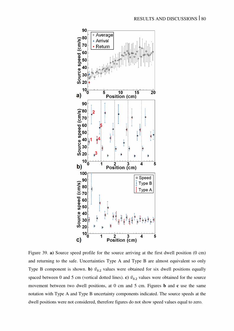
RESULTS AND DISCUSSIONS | 80
Figure 39. a) Source speed profile for the source arriving at the first dwell position (0 cm)
and returning to the safe. Uncertainties Type A and Type B are almost equivalent so only
Type B component is shown. b) . values were obtained for six dwell positions equally
spaced between 0 and 5 cm (vertical dotted lines). c) . values were obtained for the source
movement between two dwell positions, at 0 cm and 5 cm. Figures b and c use the same
notation with Type A and Type B uncertainty components indicated. The source speeds at the
dwell positions were not considered, therefore figures do not show speed values equal to zero.
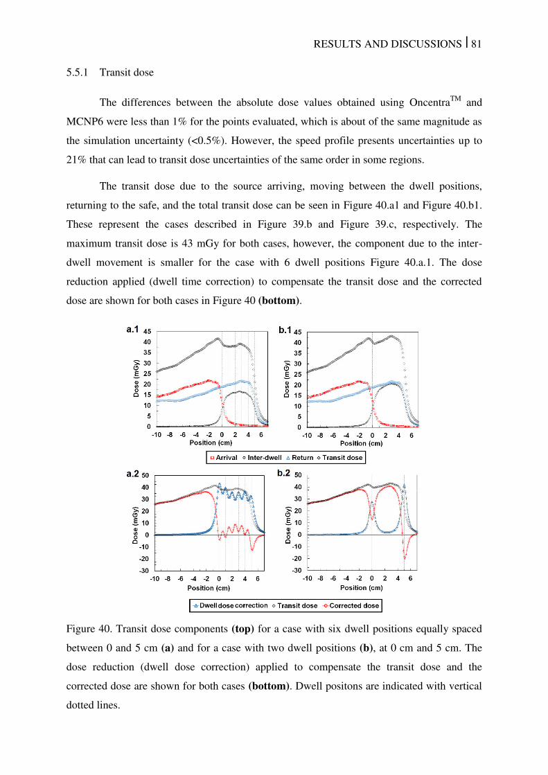
RESULTS AND DISCUSSIONS | 81
5.5.1 Transit dose
The differences between the absolute dose values obtained using OncentraTM
and
MCNP6 were less than 1% for the points evaluated, which is about of the same magnitude as
the simulation uncertainty (<0.5%). However, the speed profile presents uncertainties up to
21% that can lead to transit dose uncertainties of the same order in some regions.
The transit dose due to the source arriving, moving between the dwell positions,
returning to the safe, and the total transit dose can be seen in Figure 40.a1 and Figure 40.b1.
These represent the cases described in Figure 39.b and Figure 39.c, respectively. The
maximum transit dose is 43 mGy for both cases, however, the component due to the inter-
dwell movement is smaller for the case with 6 dwell positions Figure 40.a.1. The dose
reduction applied (dwell time correction) to compensate the transit dose and the corrected
dose are shown for both cases in Figure 40 (bottom).
Figure 40. Transit dose components (top) for a case with six dwell positions equally spaced
between 0 and 5 cm (a) and for a case with two dwell positions (b), at 0 cm and 5 cm. The
dose reduction (dwell dose correction) applied to compensate the transit dose and the
corrected dose are shown for both cases (bottom). Dwell positons are indicated with vertical
dotted lines.
RESULTS AND DISCUSSIONS | 82
The dose reduction due to the dwell time correction applied by the manufacturer was
obtained with a 0.073 s dwell time for the first position (0 cm) and dwell times between 0.047
and 0.052 s for the other dwell positions (Figure 40.a2 / video 2). The case with 2 dwell
positions (Figure 40.b2 / video 3) was simulated with 0.056 s dwell time for the first position
and 0.085 s for the last position. The correction applied by the manufacturer compensates for
the transit dose between the dwell positions for 1 cm inter-dwell distance leading to a smaller
transit dose and even to underdoses near the last dwell position (Figure 1.b1). The corrected
dose obtained with a 5 cm inter-dwell distance shows that the dwell time reduction
compensates the transit dose only near the dwell positions and also leads to underdose near
the end of the trajectory. The maximum overdose after the dwell time correction was 41
mGy, which is within 1.4% for commonly prescribed doses (3-10 Gy/fraction)146
.
5.5.2 Discussion
The periodic speed variations seem to be independent of the inter-dwell distance. For
example, the speed profile for 1 cm inter-dwell distance (Figure 39.b) is similar to the speed
profile of the first centimeter obtained with 5 cm inter-dwell distance (Figure 39.c).
Moreover, the speed profile obtained with 5 cm inter-dwell distance was used to obtain
average speeds for the first 0.25, 0.50, 1.00 and 2.50 cm of the source trajectory. All values
obtained are equivalent to the average speed profiles obtained for equivalent inter-dwell
distances (Table 8) within uncertainties. The highest average speed for the 0.5 cm inter-dwell
distance occurs due to the absence of non-programmed dwell positions for this inter-dwell
distance. In addition, the source reaches the maximum speed (Figure 39.b and 2.c) within 0.5
cm inter-dwell distance and does not reach it for a 0.25 cm inter-dwell distance, which also
explains a higher average speed for the 0.5 cm than for 0.25 cm inter-dwell distance.
The complex behavior of the source movement, including very short stops at non-
programmed positions, was also observed for another afterloader by Wojcicka et al.43
One
possible explanation for the observed variations could be attributed to a motor warm-up since
the amplitude of speed oscillations reduces with distance (Figure 39.c). It can also be due to
wire spring or another mechanical property of the equipment, which was not evaluated in this
study.
The periodic speed variations may explain differences obtained in the literature as
source speed varies significantly with source position. Studies performed with a video camera
with a lower frame rate or detectors at fixed positions would not have the required
RESULTS AND DISCUSSIONS | 83
spatial/temporal resolution to observe these effects. This explanation does not apply for
integration methods, which may indicate that differences can be due to high uncertainties
and/or different behaviors between each piece of equipment or their models. This highlighted
the importance of including transit dose component measurements in quality assurance (QA)
tests since low speed sources can lead to high transit doses.50, 146
Williamson et al. also
described a simple methodology to measure source speed using an ionization chamber and
how to estimate the transit dose that can be employed for QA tests.146
The transit dose does not seem to be significant for the obtained speed profiles. A
previous study showed that the transit dose with average speed of 30 cm/s (close to values
measured in this study) would result in transit doses up to 0.3% and 2.3% of the prescribed
dose for a gynecological and a prostate case.50
These values were obtained without any dwell
time correction so the real impact of the transit dose would be even smaller.50
On the other
hand, our results show that the transit dose is not uniformly distributed and that the transit
dose for dwell positions far apart (Figure 40.b2) were not fully corrected showing over and
underdoses. The dwell time correction applied by the manufacturer is more efficient for
smaller inter-dwell distances (Figure 40.b1). Additional dwell positions do not increase the
transit dose due to the instantaneous source stop and fast acceleration leading to high average
speed even for small inter-dwell distances.
Our findings do not apply for sources with lower acceleration or following uniform
accelerated movements42, 43, 46
for which additional dwell positions would increase the transit
time due to the source slowing down and accelerating from rest near the dwell positions.50
The impact of the number of the dwell positions may be relevant if the average speed
depends on the inter-dwell distance, which should be evaluated for each source since the
transit effect may be more relevant for slower sources.
Transit dose could also be taken into account at the treatment planning stage, instead
of attempting to correct for it during radiation delivery.

CONCLUSIONS Chapter 6
CONCLUSIONS | 85
6 CONCLUSIONS
Obtained results are relevant for HDR brachytherapy treatment planning. Although
not clinically available, most subjects described in this thesis can be assessed using
AMIGOBrachy that offers a user-friendly interface providing resources to perform dose
calculations based on MC simulation. It takes into account the body geometry, tissue
composition and applicator attenuation as recommended by TG-186. The studied cases show
good agreement with ACUROSTM
with some under and overdosing compared to TG-43U1
based dose with differences around 5% within the target volume and up to 25% within the
evaluated regions. AMIGOBrachy can improve the accuracy of the dose distribution through
a more accurate applicator representation and/or a more accurate dose calculation algorithm
that can handle tissue composition. Currently, low energy EBS for which tissue composition
is highly significant can also be simulated using the developed interface. Moreover,
AMIGOBrachy can import applicators in the CAD format and includes metal needles that are
not present in the ACUROSTM
applicator database.
CAD mesh features are applicable to Geant4 and MCNP6 MC codes, which allow the
modelling of complex brachytherapy applicator geometries in MC simulations, as an
alternative to CSG representations. Results were validated using simple cases allowing CSG
representation. For complex applicators, which do not allow straightforward CSG modelling
such as the shielded Fletcher Williamson applicator, we validated the MG method using a
modified model. For the realistic APBI balloon applicator, which has an irregular geometry
that precludes easy modelling with CSG, we have observed good agreement between
MCNP6 and Geant4. The use of MG generally entails a computation efficiency penalty
compared to simulation times for CSG with the same code, for the cases evaluated in this
work. However, simulation times depend on the Monte Carlo code and on the simulation
setup with MG being faster than CSG for some cases in the literature.147
Strategies such as
scoring a phase space at the surface of applicators could be employed to minimize the impact
of this penalty. The methods presented here can be used in the validation process of treatment
planning systems or to evaluate modifications to applicator design. The MG method should
also be equally useful in modelling other complex radiotherapy devices in external beam
radiotherapy with photons, electrons or light ions.
The AMIGOBrachy/MCNP6 capability to score Dm,m and Dw,m, mean-energy and
source spectrum is an important feature. For HDR brachytherapy with the 192
Ir isotope the
photon spectrum changes considerably inside the patient as function of distance to implant
and depending on the patient/phantom material composition. The low energy photon
CONCLUSIONS | 86
contribution to the total dose is higher in regions away from the implant. The results obtained
show that differences between Dm,m and Dw,m (SCT or LCT) can be negligible (<1%) for
some tissues as muscle and significant for other tissues with differences up to 14% for bone
in the evaluated head and neck case. The dose conversion approach (SCT or LCT) leads to
significant differences since materials with µ / � greater than 1 may have /� � less
than 1 or vice versa (Figure 1). Therefore differences between conversion factors (LCT and
SCT) are up to 28% for bone and 36% for teeth. It is essential that brachytherapy studies
explicitly mention which dose reporting quantity has been used (Dm,m, Dw,m(LCT), or
Dw,m(SCT). Of extra importance is to be aware that in some materials and locations, the
difference between Dw,m(LCT), Dw,m(SCT) and Dm,m are substantial.
Finally, transit dose component due to the source movement can be assessed once the
speed profiles are well know. The transit dose for 192
Ir HDR brachytherapy treatments can be
significant reaching more than 1.8 Gy (worst case scenario without include dwell time
corrections) and representing up to 20% of the dwell dose for the a specific region of the
prostate case analyzed in this study. The transit dose was found to be more significant for the
interstitial cases analyzed since they have lower dwell times due to de proximity between the
dwell positions and the tissue. The simple approach adopted here to reduce the transit dose
component is approximately equivalent to the one adopted by Palmer et al.10
reducing
significantly the transit dose component. Although the literature data shows a wide spread in
reported values for the source speed profile, the source speed seems to be low enough to
produce significant effects in the dose distribution, which should be taken into account.8,9,10,13
A high speed camera allowed a detailed determination of the source movement for a
Nucletron source, which can be clearly visualized with the videos available online. The dwell
time correction applied by the manufacturer (Figure 40) may lead to doses, averaged over the
volume, equivalent to the planned doses since the transit time between the dwell positions
may be fully compensated reducing the dwell times. This depends on the distances between
dwell positions, though. However, the transit dose distribution is not uniform and, ideally,
should be considered during treatment planning to optimize the dose distribution. The transit
dose correction may be greater than the transit dose leading to underdose at some regions
(Figure 40). This issue increases in importance for slower moving brachytherapy sources.
The main subjects evaluated in this study are relevant for brachytherapy treatment
planning and have the potential to improve treatment accuracy. Although not clinically
available, many of the issues described in here can be assessed with AMIGOBrachy, coupled
with a MC code.

FUTURE PERSPECTIVES
Chapter 7
FUTURE PERSPECTIVES| 88
7 FUTURE PERSPECTIVES
Relevant advances have been made in several issues to improve brachytherapy, which
show the effort of different research groups to publish around 1000 papers per year
(PubMed††
- 21 January 2015), with the term ‘brachytherapy’, between 2012 and 2014.
Moreover, efforts are also related with image segmentation, imaging techniques, artifacts
corrections and other issues that may not appear in the search since brachytherapy may not be
mentioned due to the general application of these topics. However, much still need be done to
make recent advances clinically available and to move further with unexplored issues.
Some relevant issues that need further investigations were pointed out along this
thesis and summarized below.
Although MBDCA algorithms are available, dwell times are calculated using TG-
43U1 since ACUROSTM
, ACE and MC codes are not fast enough to perform dose
optimizations. Therefore, MBDCA are used clinically only for dose recalculations.
Technical efforts are necessary to improve both computational power and software
efficiency.
Dosimetry for brachytherapy is a complex issue due to the sharp dose gradient
being disregard for several clinical centers due to the large uncertainties.
Measurements, including in-vivo dosimetry, are highly important to detect source
misplacements or dose miscalculation. To reduce experimental uncertainty some
issues should be considered: dosimeters energy dependence must be carefully
evaluated for low energies; real time positioning system should be employed.
Source speed profiles should be characterized for several afterloads since
differences in the literature are significant and can lead to negligible or highly
significant transit doses. Currently, is to clear the reason between such large
differences in the speed profile, however, this thesis demonstrate that it can lead to
non-uniform dose distribution and that more accurate corrections are necessary.
Dose report quantities (Dw,m and Dm,m) obtained using SCT or LCT differs
significantly and are patient specific due to the energy dependence of results
obtained using LCT. More studies are necessary to define standards allowing
comparison between results obtained in different centers.
†† http://www.ncbi.nlm.nih.gov/pubmed/

FUTURE PERSPECTIVES| 89
Significant advances are expected within the next few years that will lead to much
more accurate treatment planning system capable of handle tissue composition, transit dose
component and applicators during optimization. Dosimetry improvements and real time
measurements will follow these advances since accurate experimental validation of such
accurate treatments plans seems to be a logical next step.

LIST OF PUBLICATIONS
LIST OF PUBLICATIONS | 91
8 LIST OF PUBLICATIONS
8.1 Published articles
F. Ballester, J. Vijande, A.C. Tedgren, D. Granero, A. Haworth, R. Smith, F. Mourtada, G.P.
Fonseca, K. Zourari, P. Papagiannis, F.A Siebert, M.J. Rivard, R. S. Sloboda, R.M.
Thomson, F. Verhaegen, Y. Ma, L. Beaulieu, “A generic high-dose-rate Ir-192 brachytherapy
source for evaluation of model-based dose calculations beyond the TG-43 formalism,” Med
Phys 42(6), 3048 (2015)
G.P. Fonseca, A.C. Tedgren, B. Reniers, J. Nilsson, M. Person, H. Yoriyaz, F. Verhaegen,
“Dose specification for 192Ir high dose rate brachytherapy in terms of dose to water in
medium and dose to medium in medium” Phys Med Biol 60, 4565-4579 (2015)
G.P. Fonseca, R.S. Viana, M. Podesta, R.A. Rubo, C.P. de Sales, B. Reniers, H. Yoriyaz, F.
Verhaegen, "HDR (192)Ir source speed measurements using a high speed video camera,"
Med Phys 42, 412 (2015)
G.P. Fonseca, G. Landry, S. White, M. D'Amours, H. Yoriyaz, L. Beaulieu, B. Reniers, F.
Verhaegen, "The use of tetrahedral mesh geometries in Monte Carlo simulation of applicator
based brachytherapy dose distributions," Phys Med Biol 59, 5921-5935 (2014).
G.P. Fonseca, B. Reniers, G. Landry, S. White, M. Bellezzo, P.C.G. Antunes, C.P. de Sales,
E. Welteman, H. Yoriyaz, F. Verhaegen, "A medical image-based graphical platform—
Features, applications and relevance for brachytherapy," Brachytherapy 13, 632-639 (2014)
S. White, G. Landry, G. P. Fonseca, R. W. Holt, T. W. Rusch, L. Beaulieu, F. Verhaegen, B.
Reniers, “Comparison of TG-43 and TG-186 in breast irradiation using a low energy
electronic brachytherapy source”, Med. Phys. 41(6), pp. 061701 (2014)
G.P. Fonseca, G. Landry, B. Reniers, P. C. G Antunes, H. Yoriyaz, F. Verhaegen, “The
contribution from transit dose for 192Ir HDR brachytherapy treatments”, Phys. Med. Biol.
59, 1831-1844 (2014)
G. P. Fonseca, R. A. Rubo, R. A. Minamisawa, G. R. dos Santos, P. C. G. Antunes, H.
Yoriyaz, “Determination of transit dose profile for a 192Ir HDR source”, Med. Phys. 40(5),
pp. 051717-1: 051717-8 (2013)

LIST OF PUBLICATIONS | 92
8.2 Conferences
G. P. Fonseca, J. Luvizotto, T. S. Coelho, P.C.G. Antunes, P. T. D. Siqueira, H. Yoriyaz.
“Brachytherapy dose measurements in heterogeneous tissues” XIV International Symposium
on Solid State Dosimetry, Cusco, Peru, 2014.
G. P. Fonseca, B. Reniers, J. Nilsson, M. Persson, A. C. Tedgren, H. Yoriyaz, F. Verhaegen,
“Monte Carlo Simulation of HDR Ir-192 Brachytherapy Cancer Treatments”. ABS
(American Brachytherapy Society) Annual Meeting. San Diego, USA, 2014.
G. P. Fonseca, J. Luvizotto, P. C. G. Antunes, H. Yoriyaz, “Dose Measurements for an Ir-
192 Source Using Mosfets, Radiochromic Films, TLDs and Heterogeneous Tissues”. ABS
(American Brachytherapy Society) Annual Meeting. San Diego, USA, 2014.
G.P. Fonseca, P.C.G. Antunes, B. Reniers, H. Yoriyaz, F. Verhaegen. “A brachytherapy
model-based dose calculation algorithm – AMIGOBrachy”. International Nuclear Atlantic
Conference, Recife, Brazil, 2013.
G. Landry, G.P. Fonseca, S. Enger, M. d’Amours, S. White, B. Reniers, L. Beaulieu, F.
Verhaegen, The use of tetrahedral meshes and layered mass geometry in Geant4
brachytherapy applications, Bordeaux, France, 2013.
G.P. Fonseca, B. Reniers, F. Verhaegen, H. Yoriyaz. “Impact of heterogeneities in a
gynecological cancer treatment using a HDR Ir-192 source”. 2ND ESTRO forum, GENEVA,
Switzerland, 2013.
G. P. Fonseca, H. Yoriyaz, P. C. G. Antunes, P. T. D. Siqueira, R. Rubo, R. A. Minamisawa,
L. A. Ferreira, “Characterization of HDR Ir-192 source for 3D planning system”
International Nuclear Atlantic Conference – INAC, Belo Horizonte, Brazil, 2011.

CURRICULUM VITAE
CURRICULUM VITAE | 94
9 CURRICULUM VITAE
Born in Itapeva, Brazil, Gabriel Paiva Fonseca obtained a degree in physics from
University of São Paulo (USP) in 2007. He developed interest for Monte Carlo methods in
medical physics performing several experiments with linear accelerators and brachytherapy
sources using several dosimeters to benchmark calculated results. A master degree in medical
physics was obtained in 2010 developing scattering plates to increase the treatment field of a
linear accelerator to perform total skin irradiations. In 2011 he started a Ph.D in Brazil under
supervision Prof. Dr Hélio Yoriyaz joining Maastro (Maastricht University (MU) – the
Netherlands) research team in 2012 under supervision of Prof. Dr. Frank Verhaegen. He
concluded his double Ph.D, USP and MU, in 2015 performing research activities in both
countries Brazil and the Netherlands.
Main research subjects:
- Monte Carlo methods;
- Medical images (CT and MRI);
- Brachytherapy treatment planning systems;
- Experimental dosimetry using TLDs, MOSFETs and films;
- Patient specific dose calculations.

REFERENCES
REFERENCES | 96
10 REFERENCES
1 R. Nath, L.L. Anderson, G. Luxton, K.A. Weaver, J.F. Williamson, A.S. Meigooni,
"Dosimetry of interstitial brachytherapy sources: recommendations of the AAPM
Radiation Therapy Committee Task Group No. 43. American Association of
Physicists in Medicine," Med Phys 22, 209-234 (1995). 2 M.J. Rivard, B.M. Coursey, L.A. DeWerd, W.F. Hanson, M.S. Huq, G.S. Ibbott, M.G.
Mitch, R. Nath, J.F. Williamson, "Update of AAPM Task Group No. 43 Report: A
revised AAPM protocol for brachytherapy dose calculations," Med Phys 31, 633-674
(2004). 3 G. Landry, B. Reniers, L. Murrer, L. Lutgens, E.B. Gurp, J.P. Pignol, B. Keller, L.
Beaulieu, F. Verhaegen, "Sensitivity of low energy brachytherapy Monte Carlo dose
calculations to uncertainties in human tissue composition," Med Phys 37, 5188-5198
(2010). 4 S.M. Hsu, C.H. Wu, J.H. Lee, Y.J. Hsieh, C.Y. Yu, Y.J. Liao, L.C. Kuo, J.A. Liang,
D.Y. Huang, "A study on the dose distributions in various materials from an Ir-192
HDR brachytherapy source," PLoS One 7, e44528 (2012). 5 L. Beaulieu, A. Carlsson Tedgren, J.F. Carrier, S.D. Davis, F. Mourtada, M.J. Rivard,
R.M. Thomson, F. Verhaegen, T.A. Wareing, J.F. Williamson, "Report of the Task
Group 186 on model-based dose calculation methods in brachytherapy beyond the
TG-43 formalism: current status and recommendations for clinical implementation,"
Med Phys 39, 6208-6236 (2012). 6 G.P. Fonseca, B. Reniers, G. Landry, S. White, M. Bellezzo, P.C.G. Antunes, C.P. de
Sales, E. Welteman, H. Yoriyaz, F. Verhaegen, "A medical image-based graphical
platform—Features, applications and relevance for brachytherapy," Brachytherapy
13, 632-639 (2014). 7 G. Landry, M.J. Rivard, J.F. Williamson, F. Verhaegen, "Monte Carlo Methods and
Applications for Brachytherapy Dosimetry and Treatment Planning," in Monte Carlo
Techniques in Radiation Therapy, edited by J. Seco, F. Verhaegen (2013), pp. 125-
143. 8 S.A. White, G. Landry, G.P. Fonseca, R. Holt, T. Rusch, L. Beaulieu, F. Verhaegen,
B. Reniers, "Comparison of TG-43 and TG-186 in breast irradiation using a low
energy electronic brachytherapy source," Med Phys 41, 061701 (2014). 9 K.A. Gifford, J.L. Horton, T.A. Wareing, G. Failla, F. Mourtada, "Comparison of a
finite-element multigroup discrete-ordinates code with Monte Carlo for radiotherapy
calculations," Phys Med Biol 51, 2253-2265 (2006). 10
L. Petrokokkinos, K. Zourari, E. Pantelis, A. Moutsatsos, P. Karaiskos, L. Sakelliou,
I. Seimenis, E. Georgiou, P. Papagiannis, "Dosimetric accuracy of a deterministic
radiation transport based 192Ir brachytherapy treatment planning system. Part II:
Monte Carlo and experimental verification of a multiple source dwell position plan
employing a shielded applicator," Med Phys 38, 1981-1992 (2011). 11
S.A. Lloyd, W. Ansbacher, "Evaluation of an analytic linear Boltzmann transport
equation solver for high-density inhomogeneities," Med Phys 40, 011707 (2013). 12
A. Carlsson Tedgren, A. Ahnesjo, "Optimization of the computational efficiency of a
3D, collapsed cone dose calculation algorithm for brachytherapy," Med Phys 35,
1611-1618 (2008). 13
M.J. Rivard, J.L. Venselaar, L. Beaulieu, "The evolution of brachytherapy treatment
planning," Med Phys 36, 2136-2153 (2009). 14
A. Ahnesjo, "Collapsed cone convolution of radiant energy for photon dose
calculation in heterogeneous media," Med Phys 16, 577-592 (1989).
REFERENCES | 97
15 A. Carlsson Tedgren, A. Ahnesjo, "The collapsed cone superposition algorithm
applied to scatter dose calculations in brachytherapy," Med Phys 27, 2320-2332
(2000). 16
G.P. Fonseca, G. Landry, S. White, M. D'Amours, H. Yoriyaz, L. Beaulieu, B.
Reniers, F. Verhaegen, "The use of tetrahedral mesh geometries in Monte Carlo
simulation of applicator based brachytherapy dose distributions," Phys Med Biol 59,
5921-5935 (2014). 17
G.P. Fonseca, G. Landry, B. Reniers, A. Hoffmann, R.A. Rubo, P.C. Antunes, H.
Yoriyaz, F. Verhaegen, "The contribution from transit dose for (192)Ir HDR
brachytherapy treatments," Phys Med Biol 59, 1831-1844 (2014). 18
J.K. Mikell, A.H. Klopp, M. Price, F. Mourtada, "Commissioning of a grid-based
Boltzmann solver for cervical cancer brachytherapy treatment planning with shielded
colpostats," Brachytherapy 12, 645-653 (2013). 19
A. Carlsson Tedgren, A. Ahnesjo, "Accounting for high Z shields in brachytherapy
using collapsed cone superposition for scatter dose calculation," Med Phys 30, 2206-
2217 (2003). 20
H. Afsharpour, G. Landry, M. D’Amours, S. Enger, B. Reniers, E. Poon, J.-F. Carrier,
F. Verhaegen, L. Beaulieu, "ALGEBRA: ALgorithm for the heterogeneous dosimetry
based on GEANT4 for BRAchytherapy," Physics in Medicine and Biology 57, 3273
(2012). 21
E. Poon, Y. Le, J.F. Williamson, F. Verhaegen, "BrachyGUI: an adjunct to an
accelerated Monte Carlo photon transport code for patient-specific brachytherapy
dose calculations and analysis," Journal of Physics: Conference Series 102, 012018
(2008). 22
M.J. T. Goorley, T. Booth, F. Brown, J. Bull, L. J. Cox, J. Durkee, J. Elson, M.
Fensin, R. A. Forster, J. Hendricks, H. G. Hughes, R. Johns, B. Kiedrowski, R. Martz,
S. Mashnik, G. McKinney, D. Pelowitz, R. Prael, J. Sweezy, L. Waters, T. Wilcox, T.
Zukaitis, "Initial MCNP6 Release Overview," Radiation Transport and Protection
180, 298-315 (2012). 23
K.A. Gifford, J.L. Horton, E.F. Jackson, T.R. Steger, M.P. Heard, F. Mourtada, A.A.
Lawyer, G.S. Ibbott, "Comparison of Monte Carlo calculations around a Fletcher Suit
Delclos ovoid with radiochromic film and normoxic polymer gel dosimetry," Med
Phys 32, 2288-2294 (2005). 24
J. Markman, J.F. Williamson, J.F. Dempsey, D.A. Low, "On the validity of the
superposition principle in dose calculations for intracavitary implants with shielded
vaginal colpostats," Med Phys 28, 147-155 (2001). 25
K.J. Weeks, "Monte Carlo dose calculations for a new ovoid shield system for
carcinoma of the uterine cervix," Med Phys 25, 2288-2292 (1998). 26
M.J. Price, K.A. Gifford, J. Horton, A. Lawyer, P. Eifel, F. Mourtada, "Comparison of
dose distributions around the pulsed-dose-rate Fletcher–Williamson and the low-dose-
rate Fletcher–Suit–Delclos ovoids: a Monte Carlo study," Physics in Medicine and
Biology 51, 4083 (2006). 27
J.F. Williamson, "Dose calculations about shielded gynecological colpostats," Int J
Radiat Oncol Biol Phys 19, 167-178 (1990). 28
S. Agostinelli, J. Allison, K. Amako, J. Apostolakis, H. Araujo, P. Arce, M. Asai, D.
Axen, S. Banerjee, G. Barrand, F. Behner, L. Bellagamba, J. Boudreau, L. Broglia, A.
Brunengo, H. Burkhardt, S. Chauvie, J. Chuma, R. Chytracek, G. Cooperman, G.
Cosmo, P. Degtyarenko, A. Dell'Acqua, G. Depaola, D. Dietrich, R. Enami, A.
Feliciello, C. Ferguson, H. Fesefeldt, G. Folger, F. Foppiano, A. Forti, S. Garelli, S.
Giani, R. Giannitrapani, D. Gibin, J.J.G. Cadenas, I. Gonzalez, G.G. Abril, G.
Greeniaus, W. Greiner, V. Grichine, A. Grossheim, S. Guatelli, P. Gumplinger, R.
REFERENCES | 98
Hamatsu, K. Hashimoto, H. Hasui, A. Heikkinen, A. Howard, V. Ivanchenko, A.
Johnson, F.W. Jones, J. Kallenbach, N. Kanaya, M. Kawabata, Y. Kawabata, M.
Kawaguti, S. Kelner, P. Kent, A. Kimura, T. Kodama, R. Kokoulin, M. Kossov, H.
Kurashige, E. Lamanna, T. Lampen, V. Lara, V. Lefebure, F. Lei, M. Liendl, W.
Lockman, F. Longo, S. Magni, M. Maire, E. Medernach, K. Minamimoto, P.M. de
Freitas, Y. Morita, K. Murakami, M. Nagamatu, R. Nartallo, P. Nieminen, T.
Nishimura, K. Ohtsubo, M. Okamura, S. O'Neale, Y. Oohata, K. Paech, J. Perl, A.
Pfeiffer, M.G. Pia, F. Ranjard, A. Rybin, S. Sadilov, E. Di Salvo, G. Santin, T. Sasaki,
N. Savvas, Y. Sawada, S. Scherer, S. Seil, V. Sirotenko, D. Smith, N. Starkov, H.
Stoecker, J. Sulkimo, M. Takahata, S. Tanaka, E. Tcherniaev, E.S. Tehrani, M.
Tropeano, P. Truscott, H. Uno, L. Urban, P. Urban, M. Verderi, A. Walkden, W.
Wander, H. Weber, J.P. Wellisch, T. Wenaus, D.C. Williams, D. Wright, T. Yamada,
H. Yoshida, D. Zschiesche, "Geant4-a Simulation Toolkit," Nuclear Instruments &
Methods in Physics Research Section a-Accelerators Spectrometers Detectors and
Associated Equipment 506, 250-303 (2003). 29
T. Goorley, M. James, T. Booth, F. Brown, J. Bull, L.J. Cox, J. Durkee, J. Elson, M.
Fensin, R.A. Forster, J. Hendricks, H.G. Hughes, R. Johns, B. Kiedrowski, R. Martz,
S. Mashnik, G. McKinney, D. Pelowitz, R. Prael, J. Sweezy, L. Waters, T. Wilcox, T.
Zukaitis, "Initial MCNP6 release overview," Radiation Transport and Protection 180,
298-315 (2012). 30
C.M. Ma, J. Li, "Dose specification for radiation therapy: dose to water or dose to
medium?," Phys Med Biol 56, 3073-3089 (2011). 31
I.J. Chetty, B. Curran, J.E. Cygler, J.J. DeMarco, G. Ezzell, B.A. Faddegon, I.
Kawrakow, P.J. Keall, H. Liu, C.M. Ma, D.W. Rogers, J. Seuntjens, D. Sheikh-
Bagheri, J.V. Siebers, "Report of the AAPM Task Group No. 105: Issues associated
with clinical implementation of Monte Carlo-based photon and electron external beam
treatment planning," Med Phys 34, 4818-4853 (2007). 32
M.J. Rivard, L. Beaulieu, F. Mourtada, "Enhancements to commissioning techniques
and quality assurance of brachytherapy treatment planning systems that use model-
based dose calculation algorithms," Med Phys 37, 2645-2658 (2010). 33
G. Landry, B. Reniers, J.-P. Pignol, L. Beaulieu, F. Verhaegen, "The difference of
scoring dose to water or tissues in Monte Carlo dose calculations for low energy
brachytherapy photon sources," Med Phys 38, 1526-1533 (2011). 34
A. Carlsson Tedgren, G.A. Carlsson, "Specification of absorbed dose to water using
model-based dose calculation algorithms for treatment planning in brachytherapy,"
Phys Med Biol 58, 2561-2579 (2013). 35
H.H. Liu, P. Keall, W.R. Hendee, "Dm rather than Dw should be used in Monte Carlo
treatment planning," Med Phys 29, 922-924 (2002). 36
R.M. Thomson, A.C. Tedgren, J.F. Williamson, "On the biological basis for
competing macroscopic dose descriptors for kilovoltage dosimetry: cellular dosimetry
for brachytherapy and diagnostic radiology," Phys Med Biol 58, 1123-1150 (2013). 37
L. Lindborg, M. Hultqvist, A. Carlsson Tedgren, H. Nikjoo, "Lineal energy and
radiation quality in radiation therapy: model calculations and comparison with
experiment," Phys Med Biol 58, 3089-3105 (2013). 38
S.A. Enger, A. Ahnesjo, F. Verhaegen, L. Beaulieu, "Dose to tissue medium or water
cavities as surrogate for the dose to cell nuclei at brachytherapy photon energies,"
Phys Med Biol 57, 4489-4500 (2012). 39
M.J. Berger, J.H. Hubbell, S.M. Seltzer, J. Chang, J.S. Coursey, R. Sukumar, D.S.
Zucker, "XCOM: Photon Cross Section Database (version 1.3)," (NIST,
Gaithersburg, MD, 2005).
REFERENCES | 99
40 M.J. Berger, Coursey, J.S., Zucker, M.A., and Chang, J, "ESTAR, PSTAR, and
ASTAR: Computer Programs for Calculating Stopping-Power and Range Tables for
Electrons, Protons, and Helium Ions (version 1.2.3)," (National Institute of Standards
and Technology, Gaithersburg, MD., 2005). 41
G.P. Fonseca, R.A. Rubo, R.A. Minamisawa, G.R. dos Santos, P.C. Antunes, H.
Yoriyaz, "Determination of transit dose profile for a (192)Ir HDR source," Med Phys
40, 051717 (2013). 42
A. Palmer, B. Mzenda, "Performance assessment of the BEBIG MultiSource high
dose rate brachytherapy treatment unit," Phys Med Biol 54, 7417-7434 (2009). 43
J.B. Wojcicka, R. Yankelevich, F. Trichter, D.P. Fontenla, "Comparison of the transit
dose components and source kinematics of three high dose rate afterloading systems,"
Med Dosim 24, 61-65 (1999). 44
T.P. Wong, W. Fernando, P.N. Johnston, I.F. Bubb, "Transit dose of an Ir-192 high
dose rate brachytherapy stepping source," Phys Med Biol 46, 323-331 (2001). 45
N. Sahoo, "Measurement of transit time of a remote after-loading high dose rate
brachytherapy source," Med Phys 28, 1786-1790 (2001). 46
R.A. Minamisawa, R.A. Rubo, R.M. Seraide, J.R. Rocha, A. Almeida, "Direct
measurement of instantaneous source speed for a HDR brachytherapy unit using an
optical fiber based detector," Med Phys 37, 5407-5411 (2010). 47
K.T. Bastin, M.B. Podgorsak, B.R. Thomadsen, "The transit dose component of high
dose rate brachytherapy: direct measurements and clinical implications," Int J Radiat
Oncol Biol Phys 26, 695-702 (1993). 48
R. Das, J. Venselaar, "Standard Technology in Brachytherapy," in Comprehensive
Brachytherapy: Physical and Clinical Aspects, edited by J. Venselaar, A.S. Meigooni,
D. Baltas, P.J. Hoskin (CRC Press, 2012). 49
T.E. Booth, J.T. Goorley, A. Sood, F.B. Brown, H.G. Hughes, J.E. Sweezy, J.S. Bull,
R. Martz, A. Zukaitis, R.A. Forster, R.E. Prael, R.C. Little, M.C. White, M.B. Lee, H.
Trellue, S.M. Girard, "MCNP—A General Monte Carlo N-Particle Transport Code -
Volume I: Overview and Theory," (2003). 50
G.P. Fonseca, G. Landry, B. Reniers, A. Hoffmann, R.A. Rubo, P.C.G. Antunes, H.
Yoriyaz, F. Verhaegen, "The contribution from transit dose for 192 Ir HDR
brachytherapy treatments," Physics in Medicine and Biology 59, 1831-1834 (2014). 51
G.P. Fonseca, R.S. Viana, M. Podesta, R.A. Rubo, C.P. de Sales, B. Reniers, H.
Yoriyaz, F. Verhaegen, "HDR (192)Ir source speed measurements using a high speed
video camera," Med Phys 42, 412 (2015). 52
H. Bequerel, P. Curie, "Action physiologique des rayons du radium," Vol. C.R. T 132
(Académie des Sciences, Paris, 1901), pp. 1289–1291. 53
D. H, P. Bloch, "Note sur le traitement du lupus érythèmateux par des applications de
radium," Ann. Dermatol. Syphil 2, 986-988 (1901). 54
M. Cleaves, "Radium: with a preliminary note on radium rays in the treatment of
cancer," Med Rec 64, 601-606 (1903). 55
R. Abbe, "Notes on the physiologic and therapeutic action of radium," Wash. Med
Ann 2 (1904). 56
J.W. Morton, "Treatment of cancer by the x-ray, with remarks on the use of radium,"
Int J Surg 14, 289-300 (1903). 57
R. Barakat, M.E. Randall, M. Markman, Principles and Practice of Gynecologic
Oncology, 5 ed. (Lippincott Williams & Wilkins, Philadelphia, 2009). 58
R. Abbe, "The use of radium in malignant disease," Lancet 2, 524-527 (1913). 59
U.K. Henschke, "A technique for permanent implantation of radioisotopes,"
Radiology 68, 256 (1957).
REFERENCES | 100
60 U.K. Henschke, "Interstitial implantation in the treatment of primary bronchogenic
carcinoma," A,. J. Roentgenol. 79, 981-987 (1958). 61
M. Brucer, "Therapeutic potentialities of radioisotopes," Merck Rep 61, 9-15 (1952). 62
J.F. Williamson, "Brachytherapy technology and physics practice since 1950: a half-
century of progress," Phys Med Biol 51, R303-325 (2006). 63
T. Palmqvist, A. Dybdahl Wanderas, A.B. Langeland Marthinsen, M. Sundset, I.
Langdal, S. Danielsen, I. Toma-Dasu, "Dosimetric evaluation of manually and
inversely optimized treatment planning for high dose rate brachytherapy of cervical
cancer," Acta Oncol 53, 1012-1018 (2014). 64
D.Y. Han, M.J. Webster, D.J. Scanderbeg, C. Yashar, D. Choi, B. Song, S. Devic, A.
Ravi, W.Y. Song, "Direction-modulated brachytherapy for high-dose-rate treatment
of cervical cancer. I: theoretical design," Int J Radiat Oncol Biol Phys 89, 666-673
(2014). 65
I. Thibault, M.C. Lavallee, S. Aubin, N. Laflamme, E. Vigneault, "Inverse-planned
gynecologic high-dose-rate interstitial brachytherapy: clinical outcomes and dose--
volume histogram analysis," Brachytherapy 11, 181-191 (2012). 66
B.R. Thomadsen, J.F. Williamson, M.J. Rivard, A.S. Meigooni, "Anniversary paper:
past and current issues, and trends in brachytherapy physics," Med Phys 35, 4708-
4723 (2008). 67
D.C. Medich, M.A. Tries, J.J. Munro, 2nd, "Monte Carlo characterization of an
ytterbium-169 high dose rate brachytherapy source with analysis of statistical
uncertainty," Med Phys 33, 163-172 (2006). 68
R. Guerrero, J.F. Almansa, J. Torres, A.M. Lallena, "Dosimetric characterization of
the (60)Co BEBIG Co0.A86 high dose rate brachytherapy source using PENELOPE,"
Phys Med 30, 960-967 (2014). 69
W.J. Meredith, "Radiotherapeutic physics: V. Dosage control in interstitial gamma-
ray therapy," Br. J. Radiol 24, 380-384 (1951). 70
N. Suntharalingam, E.B. Podgorska, H. T¨olli, "Brachytherapy: Physical and Clinical
Aspects," (International Atomic Energy Agency, Vienna) (2005). 71
E.H. Quimby,"The calculation of dosage in interstitial radium therapy," Am. J.
Roentgenol., Radium Ther. Nucl. Med 70, 739-740 (1953). 72
J.F. Williamson, "The Sievert integral revisited: evaluation and extension to 125I,
169Yb, and 192Ir brachytherapy sources," Int J Radiat Oncol Biol Phys 36, 1239-
1250 (1996). 73
J.F. Williamson, "Monte Carlo-based dose-rate tables for the Amersham CDCS.J and
3M model 6500 137Cs tubes," Int J Radiat Oncol Biol Phys 41, 959-970 (1998). 74
W.M. Butler, W.S. Bice, Jr., L.A. DeWerd, J.M. Hevezi, M.S. Huq, G.S. Ibbott, J.R.
Palta, M.J. Rivard, J.P. Seuntjens, B.R. Thomadsen, "Third-party brachytherapy
source calibrations and physicist responsibilities: report of the AAPM Low Energy
Brachytherapy Source Calibration Working Group," Med Phys 35, 3860-3865 (2008). 75
R.E.P. Taylor, G. Yegin, D.W.O. Rogers, "Benchmarking BrachyDose: Voxel based
EGSnrc Monte Carlo calculations of TG-43 dosimetry parameters," Med Phys 34,
445-457 (2007). 76
R.E. Taylor, D.W. Rogers, "EGSnrc Monte Carlo calculated dosimetry parameters for
192Ir and 169Yb brachytherapy sources," Med Phys 35, 4933-4944 (2008). 77
G.M. Daskalov, E. Loffler, J.F. Williamson, "Monte Carlo-aided dosimetry of a new
high dose-rate brachytherapy source," Med Phys 25, 2200-2208 (1998). 78
K.R. Russell, A.K. Tedgren, A. Ahnesjo, "Brachytherapy source characterization for
improved dose calculations using primary and scatter dose separation," Med Phys 32,
2739-2752 (2005).

REFERENCES | 101
79 Y. Yu, L.L. Anderson, Z. Li, D.E. Mellenberg, R. Nath, M.C. Schell, F.M. Waterman,
A. Wu, J.C. Blasko, "Permanent prostate seed implant brachytherapy: report of the
American Association of Physicists in Medicine Task Group No. 64," Med Phys 26,
2054-2076 (1999). 80
H.H. Holm, N. Juul, J.F. Pedersen, H. Hansen, I. Stroyer, "Transperineal 125iodine
seed implantation in prostatic cancer guided by transrectal ultrasonography," J Urol
130, 283-286 (1983). 81
M. Riccabona, J. Hammer, A. Schorn, "[Percutaneous, perineal, ultrasound-controlled
implantation of 125iodine in prostatic cancer: technics, report of initial experiences
and comparison with the retropubic method of implantation]," Urologe A 26, 15-21
(1987). 82
J.C. Blasko, P.D. Grimm, H. Ragde, "Brachytherapy and Organ Preservation in the
Management of Carcinoma of the Prostate," Semin Radiat Oncol 3, 240-249 (1993). 83
H. Jiang, J. Seco, H. Paganetti, "Effects of Hounsfield number conversion on CT
based proton Monte Carlo dose calculations," Med Phys 34, 1439-1449 (2007). 84
J.F. Williamson, S. Li, S. Devic, B.R. Whiting, F.A. Lerma, "On two-parameter
models of photon cross sections: Application to dual-energy CT imaging," Med Phys
33, 4115-4129 (2006). 85
G. Landry, B. Reniers, P.V. Granton, B. van Rooijen, L. Beaulieu, J.E. Wildberger, F.
Verhaegen, "Extracting atomic numbers and electron densities from a dual source
dual energy CT scanner: experiments and a simulation model," Radiother Oncol 100,
375-379 (2011). 86
G. Landry, P.V. Granton, B. Reniers, M.C. Ollers, L. Beaulieu, J.E. Wildberger, F.
Verhaegen, "Simulation study on potential accuracy gains from dual energy CT tissue
segmentation for low-energy brachytherapy Monte Carlo dose calculations," Phys
Med Biol 56, 6257-6278 (2011). 87
D. Fontanarosa, S. Pesente, F. Pascoli, D. Ermacora, I.A. Rumeileh, F. Verhaegen, "A
speed of sound aberration correction algorithm for curvilinear ultrasound transducers
in ultrasound-based image-guided radiotherapy," Phys Med Biol 58, 1341-1360
(2013). 88
M. Bazalova, L. Beaulieu, S. Palefsky, F. Verhaegen, "Correction of CT artifacts and
its influence on Monte Carlo dose calculations," Med Phys 34, 2119-2132 (2007). 89
C. Xu, F. Verhaegen, D. Laurendeau, S.A. Enger, L. Beaulieu, "An algorithm for
efficient metal artifact reductions in permanent seed," Med Phys 38, 47-56 (2011). 90
M. Yazdi, L. Gingras, L. Beaulieu, "An adaptive approach to metal artifact reduction
in helical computed tomography for radiation therapy treatment planning:
experimental and clinical studies," Int J Radiat Oncol Biol Phys 62, 1224-1231
(2005). 91
D. Xia, J.C. Roeske, L. Yu, C.A. Pelizzari, A.J. Mundt, X. Pan, "A hybrid approach to
reducing computed tomography metal artifacts in intracavitary brachytherapy,"
Brachytherapy 4, 18-23 (2005). 92
M. Gaudreault, B. Reniers, G. Landry, F. Verhaegen, L. Beaulieu, "Dose perturbation
due to catheter materials in high-dose-rate interstitial (192)Ir brachytherapy,"
Brachytherapy 13, 627-631 (2014). 93
K.A. Gifford, J.L. Horton, Jr., E.F. Jackson, T.R. Steger, 3rd, M.P. Heard, F.
Mourtada, A.A. Lawyer, G.S. Ibbott, "Comparison of Monte Carlo calculations
around a Fletcher Suit Delclos ovoid with radiochromic film and normoxic polymer
gel dosimetry," Med Phys 32, 2288-2294 (2005). 94
Z. Tian, Y.J. Graves, X. Jia, S.B. Jiang, "Automatic commissioning of a GPU-based
Monte Carlo radiation dose calculation code for photon radiotherapy," Phys Med Biol
59, 6467-6486 (2014).
REFERENCES | 102
95 Y.S. Yeom, J.H. Jeong, M.C. Han, C.H. Kim, "Tetrahedral-mesh-based computational
human phantom for fast Monte Carlo dose calculations," Phys Med Biol 59, 3173-
3185 (2014). 96
A.A. Nunn, S.D. Davis, J.A. Micka, L.A. DeWerd, "LiF:Mg,Ti TLD response as a
function of photon energy for moderately filtered x-ray spectra in the range of 20-250
kVp relative to 60Co," Med Phys 35, 1859-1869 (2008). 97
R.S. Viana, G.A. Agasthya, H. Yoriyaz, A.J. Kapadia, "3D element imaging using
NSECT for the detection of renal cancer: a simulation study in MCNP," Phys Med
Biol 58, 5867-5883 (2013). 98
A.E. Nahum, "Water/air mass stopping power ratios for megavoltage photon and
electron beams," Physics in Medicine and Biology 23, 24 (1978). 99
A.E. Nahum, M. Kristensen, "Calculated response and wall correction factors for
ionization chambers exposed to 60Co gamma rays," Med Phys 9, 925-927 (1982). 100
D.W.O. Rogers, "How accurately can EGS4/PRESTA calculate ion‐chamber
response?," Med Phys 20, 319-323 (1993). 101
D.W. Rogers, "Fifty years of Monte Carlo simulations for medical physics," Phys
Med Biol 51, R287-301 (2006). 102
J. Baró, J. Sempau, J.M. Fernández-Varea, F. Salvat, "PENELOPE: An algorithm for
Monte Carlo simulation of the penetration and energy loss of electrons and positrons
in matter," Nuclear Instruments and Methods in Physics Research Section B: Beam
Interactions with Materials and Atoms 100, 31-46 (1995). 103
S. Jan, G. Santin, D. Strul, S. Staelens, K. Assie, D. Autret, S. Avner, R. Barbier, M.
Bardies, P.M. Bloomfield, D. Brasse, V. Breton, P. Bruyndonckx, I. Buvat, A.F.
Chatziioannou, Y. Choi, Y.H. Chung, C. Comtat, D. Donnarieix, L. Ferrer, S.J. Glick,
C.J. Groiselle, D. Guez, P.F. Honore, S. Kerhoas-Cavata, A.S. Kirov, V. Kohli, M.
Koole, M. Krieguer, D.J. van der Laan, F. Lamare, G. Largeron, C. Lartizien, D.
Lazaro, M.C. Maas, L. Maigne, F. Mayet, F. Melot, C. Merheb, E. Pennacchio, J.
Perez, U. Pietrzyk, F.R. Rannou, M. Rey, D.R. Schaart, C.R. Schmidtlein, L. Simon,
T.Y. Song, J.M. Vieira, D. Visvikis, R. Van de Walle, E. Wieers, C. Morel, "GATE: a
simulation toolkit for PET and SPECT," Phys Med Biol 49, 4543-4561 (2004). 104
V. Krishaswamy, "Calculation of the dose distribution about californium-252 needles
in tissue," Radiology 98, 155-160 (1971). 105
L.L. Meisberger, R.J. Keller, R.J. Shalek, "The effective attenuation in water of the
gamma rays of gold 198, iridium 192, cesium 137, radium 226, and cobalt 60,"
Radiology 90, 953-957 (1968). 106
A. Kirov, J.F. Williamson, A.S. Meigooni, Y. Zhu, "TLD, diode and Monte Carlo
dosimetry of an 192Ir source for high dose-rate brachytherapy," Phys Med Biol 40,
2015-2036 (1995). 107
R.K. Valicenti, A.S. Kirov, A.S. Meigooni, V. Mishra, R.K. Das, J.F. Williamson,
"Experimental validation of Monte Carlo dose calculations about a high-intensity Ir-
192 source for pulsed dose-rate brachytherapy," Med Phys 22, 821-829 (1995). 108
J.F. Williamson, "Comparison of measured and calculated dose rates in water near I-
125 and Ir-192 seeds," Med Phys 18, 776-786 (1991). 109
J.F. Williamson, H. Perera, Z. Li, W.R. Lutz, "Comparison of calculated and
measured heterogeneity correction factors for 125I, 137Cs, and 192Ir brachytherapy
sources near localized heterogeneities," Med Phys 20, 209-222 (1993). 110
H. Perera, J.F. Williamson, Z. Li, V. Mishra, A.S. Meigooni, "Dosimetric
characteristics, air-kerma strength calibration and verification of Monte Carlo
simulation for a new Ytterbium-169 brachytherapy source," Int J Radiat Oncol Biol
Phys 28, 953-970 (1994).
REFERENCES | 103
111 R.K. Das, D. Keleti, Y. Zhu, A.S. Kirov, A.S. Meigooni, J.F. Williamson, "Validation
of Monte Carlo dose calculations near 125I sources in the presence of bounded
heterogeneities," Int J Radiat Oncol Biol Phys 38, 843-853 (1997). 112
P. Papagiannis, E. Pantelis, P. Karaiskos, "Current state of the art brachytherapy
treatment planning dosimetry algorithms," Br J Radiol 87, 20140163 (2014). 113
J.T. Goorley, M.R. James, T.E. Booth, F.B. Brown, J.S. Bull, L.J. Cox, J.W.J.
Durkee, J.S. Elson, M.L. Fensin, R.A.I. Forster, J.S. Hendricks, H.G.I. Hughes, R.C.
Johns, B.C. Kiedrowski, R. Martz, R. L., S.G. Mashnik, G.W. McKinney, D.B.
Pelowitz, R.E. Prael, J.E. Sweezy, L.S. Waters, T. Wilcox, A.J. Zukaitis, "Initial
MCNP6 Release Overview - MCNP6 version 1.0," 2013). 114
ICRU Radiation Quantities and Units, Report 33 of the International Commission on
Radiation Units and Measurements (Bethesda, MD) (1980). 115
C.M. Baglin, "Nuclear Data Sheets for A = 192," Nuclear Data Sheets 113, 1871-
2111 (2012). 116
C.G.a.J.-F. Remacle, "Gmsh: a three-dimensional finite element mesh generator with
built-in pre- and post-processing facilities," International Journal for Numerical
Methods in Engineering 79, 1309-1331 (2009). 117
R.L. Martz, "The MCNP6 Book On Unstructured Mesh Geometry: User’s Guide," (2012).
118 F. Ballester, D. Granero, J. Perez-Calatayud, C.S. Melhus, M.J. Rivard, "Evaluation
of high-energy brachytherapy source electronic disequilibrium and dose from emitted
electrons," Med Phys 36, 4250-4256 (2009). 119
R. Wang, X.A. Li, "Dose characterization in the near-source region for two high dose
rate brachytherapy sources," Med Phys 29, 1678-1686 (2002). 120
M.J. Rivard, S.D. Davis, L.A. DeWerd, T.W. Rusch, S. Axelrod, "Calculated and
measured brachytherapy dosimetry parameters in water for the Xoft Axxent X-Ray
Source: an electronic brachytherapy source," Med Phys 33, 4020-4032 (2006). 121
J.F. Williamson, "Monte Carlo evaluation of kerma at a point for photon transport
problems," Med Phys 14, 567-576 (1987). 122
M.J. Berger, J.S. Coursey, M.A. Zucker and J. Chang, "ESTAR, PSTAR, and
ASTAR: Computer Programs for Calculating Stopping-Power and Range Tables for
Electrons, Protons, and Helium Ions," (Version 1.2.3) (Gaithersburg, MD: NIST)
(2005). 123
ICRU "Stopping Powers for Electrons and Positions," Report 37, (international
Comission on Radiation units and Masurements, Bethesda, MD) (1984). 124
S.A. Enger, G. Landry, M. D'Amours, F. Verhaegen, L. Beaulieu, M. Asai, J. Perl,
"Layered mass geometry: a novel technique to overlay seeds and applicators onto
patient geometry in Geant4 brachytherapy simulations," Phys Med Biol 57, 6269-
6277 (2012). 125
C.M. Poole, I. Cornelius, J.V. Trapp, C.M. Langton, "A CAD interface for
GEANT4," Australasian Physical & Engineering Sciences in Medicine 35, 329-334
(2012). 126
C.M. Poole, I. Cornelius, J.V. Trapp, C.M. Langton, "Fast Tessellated Solid
Navigation in GEANT4," Nuclear Science, IEEE Transactions on 59, 1695-1701
(2012). 127
V.O. Zilio, O.P. Joneja, Y. Popowski, A. Rosenfeld, R. Chawla, "Absolute depth-
dose-rate measurements for an 192Ir HDR brachytherapy source in water using
MOSFET detectors," Med Phys 33, 1532-1539 (2006). 128
A. Fogliata, G. Nicolini, A. Clivio, E. Vanetti, L. Cozzi, "Dosimetric evaluation of
Acuros XB Advanced Dose Calculation algorithm in heterogeneous media,"
Radiation Oncology 6, 82 (2011).

REFERENCES | 104
129 ICRP, "Adult Reference Computational Phantoms. ICRP Publication 110," Ann.
ICRP 39 (2) (2009). 130
J. Perez-Calatayud, D. Granero, F. Ballester, "Phantom size in brachytherapy source
dosimetric studies," Med Phys 31, 2075-2081 (2004). 131
D. Liu, E. Poon, M. Bazalova, B. Reniers, M. Evans, T. Rusch, F. Verhaegen,
"Spectroscopic characterization of a novel electronic brachytherapy system," Phys
Med Biol 53, 61-75 (2008). 132
M.J. Rivard, S.D. Davis, L.A. DeWerd, T.W. Rusch, S. Axelrod, "Calculated and
measured brachytherapy dosimetry parameters in water for the Xoft Axxent X-Ray
Source: an electronic brachytherapy source," Med Phys 33, 4020-4032 (2006). 133
L. Petrokokkinos, K. Zourari, E. Pantelis, A. Moutsatsos, P. Karaiskos, L. Sakelliou,
I. Seimenis, E. Georgiou, P. Papagiannis, "Dosimetric accuracy of a deterministic
radiation transport based 192Ir brachytherapy treatment planning system. Part II:
Monte Carlo and experimental verification of a multiple source dwell position plan
employing a shielded applicator," Med Phys 38, 1981-1992 (2011). 134
D. Thain, T. Tannenbaum, M. Livny, "Distributed computing in practice: the Condor
experience: Research Articles," Concurr. Comput. : Pract. Exper. 17, 323-356 (2005). 135
G.P. Fonseca, B. Reniers, G. Landry, S. White, M. Bellezzo, P.C. Antunes, C.P. de
Sales, E. Welteman, H. Yoriyaz, F. Verhaegen, "A medical image-based graphical
platform-Features, applications and relevance for brachytherapy," Brachytherapy
(2014). 136
C.S. Calcina, A. de Almeida, J.R. Rocha, F.C. Abrego, O. Baffa, "Ir-192 HDR transit
dose and radial dose function determination using alanine/EPR dosimetry," Phys Med
Biol 50, 1109-1117 (2005). 137
"Planning system manual, ONCENTRA®MasterPlan v3.3 Physics and Algorithms,"
Report No. 192.718ENG-04. 138
ICRP, “Report on the Task Group on Reference Man,” Ann. ICRP 23 (1975) 139
T. Goorley, "MCNP5 Tally Enhancements for Lattices," Los Alamos, NM: National
Laboratory) (2004). 140
B. Reniers, D. Liu, T. Rusch, F. Verhaegen, "Calculation of relative biological
effectiveness of a low-energy electronic brachytherapy source," Phys Med Biol 53,
7125-7135 (2008). 141
A.C. Tedgren, A. Hedman, J.E. Grindborg, G.A. Carlsson, "Response of LiF:Mg,Ti
thermoluminescent dosimeters at photon energies relevant to the dosimetry of
brachytherapy (<1 MeV)," Med Phys 38, 5539-5550 (2011). 142
J.L.G. Massillon, A. Cabrera-Santiago, R. Minniti, M. O'Brien, C.G. Soares,
"Influence of phantom materials on the energy dependence of LiF:Mg,Ti
thermoluminescent dosimeters exposed to 20-300 kV narrow x-ray spectra, 137Cs
and 60Co photons," Phys Med Biol 59, 4149-4166 (2014). 143
C. Ehringfeld, S. Schmid, K. Poljanc, C. Kirisits, H. Aiginger, D. Georg, "Application
of commercial MOSFET detectors for in vivo dosimetry in the therapeutic x-ray range
from 80 kV to 250 kV," Phys Med Biol 50, 289-303 (2005). 144
B. Reniers, G. Landry, R. Eichner, A. Hallil, F. Verhaegen, "In vivo dosimetry for
gynaecological brachytherapy using a novel position sensitive radiation detector:
feasibility study," Med Phys 39, 1925-1935 (2012). 145
P.V. Houdek, J.G. Schwade, X. Wu, V. Pisciotta, J.A. Fiedler, C.F. Serago, A.M.
Markoe, A.A. Abitbol, A.A. Lewin, P.G. Braunschweiger, et al., "Dose determination
in high dose-rate brachytherapy," Int J Radiat Oncol Biol Phys 24, 795-801 (1992). 146
J.F. Williamson, G.A. Ezzell, A. Olch, B.R. Tomadsen, "Quality Assurance for High
Dose Rate Brachytherapy," in High Dose Rate Brachytherapy: A Textbook, edited by
S. Nag (Futura Pub Co), pp. 147-212 (1994)

REFERENCES | 105
147 Y.S. Yeom, J.H. Jeong, M.C. Han, C.H. Kim, "Tetrahedral-mesh-based computational
human phantom for fast Monte Carlo dose calculations," Physics in Medicine and
Biology 59, 3173 (2014).

VALORIZATION ADDENDUM
VALORIZATION ADDENDUM | 107
11 VALORIZATION ADDENDUM
Brachytherapy has been under continuous development for more than a century now,
improved outcomes result from increased accuracy in radiation delivery. Currently, the
conventional water based dose formalism, TG-43U1, is being replaced with more accurate
models. However, important technical challenges need to be overcome before a definitive
clinical implementation of the recently developed technologies can be realised. Some of
these aspects were evaluated in this thesis, aiming to provide knowledge and resources to
move towards more accurate treatment plans and radiation dose delivery.
This study was performed in two countries, Brazil and the Netherlands, in
collaboration with hospitals from Sweden and Belgium. It demonstrates an international
interest in brachytherapy and the potential application of the acquired knowledge.
11.1 Innovation
This thesis aims to improve brachytherapy treatment and can be divided into four
specific novel subjects.
11.1.1 Model Based Dose Calculation Algorithm
AMIGOBrachy (A Medical Image-based Graphical platfOrm - Brachytherapy
module) is software developed to create an efficient and powerful user-friendly graphical
interface, needed to integrate clinical treatment plans with MC simulations. It does this by
providing the main resources required to process and edit images, import and edit treatment
plans, as well as set MC simulation parameters. It is the first software to provide all these
functionalities combined with the capability to import and verify treatment plans created with
commercial TPS (Treatment Planning System) through MC calculations. In addition,
AMIGOBrachy can account for source movement, calculate different dose reporting
quantities, mean energy and photon energy spectrum. All of these features are not currently
available in typical clinical practice.
VALORIZATION ADDENDUM | 108
11.1.2 CAD-Mesh geometries
The modelling of complex brachytherapy applicators can be suboptimal when using
voxel based geometry, due to the sub-voxel dimensions of specific components. In addition,
applicator modelling using constructive solid geometry can be tedious, and may not allow
complete fidelity or may be highly impractical, as is the case for deformable balloon
applicators employed in accelerated partial breast irradiation (APBI).
Some modelling limitations can be avoided with CAD-Mesh geometries that can be
imported by recent versions of general purpose MC codes. This thesis is the first study to
evaluate CAD-Mesh models of brachytherapy applicators through MC simulations.
Moreover, it is the most accurate method to model deformable applicators (APBI balloon
applicator – item 4.3) available thus far.
11.1.3 Dose specification
Dose reporting quantities are especially relevant since the transition from the TG-
43U1 formalism to more accurate dose calculation algorithms will make both Dm,m and Dw,m
quantities available in typical clinical practice very soon. Differences between dose reporting
in terms of Dm,m and Dw,m have been discussed in the literature with arguments in favor and
against both quantities. However, this is the first study to show how differences in the photon
energy spectrum inside of the patient can affect the relation between Dm,m and Dw,m for
different tissues. This study can substantially contribute to future judgements regarding which
quantity should be adopted as the standard in clinical practice.
11.1.4 Transit dose
The dose component due to source movement inside of the patient is, surprisingly, not
well known. It is dependent upon the source speed profile which is not well established, with
reported differences of up to a factor 10 (depending on the measurement methodology). Such
large differences in the speed values lead to either negligible or highly significant transit
doses, which was assessed for clinical cases for the first time in this thesis. These results
indicate the importance to perform more accurate source speed profile measurements, which
were conducted in this study for one afterloader model. Speed profiles were obtained using a
high speed video camera capable of recording up to 960 fps leading to the most accurate
source speed values available to date.
VALORIZATION ADDENDUM | 109
11.2 Clinical relevance
Patient safety is a priority for medical treatments with hospitals and research centers
working exhaustively to improve the actual treatment conditions. However, brachytherapy is
particularly prone to treatment errors, due to the lack of integrated imaging in the treatment
room, coupled with the high dose gradients employed in the vicinity of radiosensitive healthy
tissues and due to simplified dose calculation models. Furthermore, treatment plans obtained
from commercial TPS are not commonly verified using alternative methods such as Monte
Carlo. There is both a significant risk to underdose the tumor, and to overdose the healthy
tissues.
The software developed, AMIGOBrachy (items 4.2 and 5.1), has a user friendly
interface that can be readily adopted in clinical practice as an auxiliary dose calculation
engine. It would provide an independent validation method with the possibility to account for
applicators, tissues composition and densities. The clinical cases evaluated with
AMIGOBrachy/MCNP6 show under and overdosing compared to TG-43U1 (item 4.2.4). The
results obtained prompted the replacement of hollow cylindrical applicators at one hospital,
due to a 5% target overdose concern in gynaecological cases. It was the first direct clinical
application of this thesis and illustrates how treatment accuracy can be improved, sometimes,
by adopting simple measures.
Finally, we provide a novel method to simulate deformable brachytherapy applicators
(APBI balloon applicator – item 4.3) that cannot be modelled with conventional analytical
geometry. The CAD-Mesh feature is also an alternative to model rigid brachytherapy
applicators and may be a suitable option when the applicator model is provided by the
manufacturer. Although the effect of the applicator can be significant (item 5.2), it is
currently not taken into account by TPS based on the TG-43U1 formalism.
11.3 Societal relevance
The scientific findings discussed in this thesis can significantly improve dose
calculation accuracy and provide relevant information that can be related to RBE effects and
patient outcome. Therefore, in the short term, treatment plans can be more accurate by
accounting for applicators, tissue composition, densities and other treatment complexities. In
the longer term, different dose reporting quantities and mean energy or the energy spectrum
VALORIZATION ADDENDUM | 110
can be assessed and related to patient outcomes once more data on these quantities becomes
available.
Brachytherapy is widely employed worldwide due to good outcomes. However, the
technology currently available can move the current standards towards even better outcomes.
If translated into clinical practice, the developments achieved in this thesis would provide a
significant contribution to this process.
Significant efforts were made to incorporate scientific advances into AMIGOBrachy
so that they are available to the radiotherapy community. The study of different dose
reporting quantities is an example of such an effort. Additionally, a physical discussion with
quantitative values for dose reporting quantities were provided for a clinical case, the
capability to score these quantities are part of AMIGOBrachy and can be used for any clinical
case.
11.4 Commercial relevance
AMIGOBrachy may become part of a commercial product in the near future which
would lead to revenue in the form of royalties, professional support service and training
courses.