


Línguas
Páginas
Legal


Eduardo José Tanque de Pádua Cruz
Parallel Interactive Ray Tracing andExploiting Spatial Coherence
Edua
rdo
José
Tan
que
de P
ádua
Cru
z
Janeiro de 2013UM
inho
| 2
013
Para
llel I
nter
activ
e Ra
y Tr
acin
g an
dEx
ploi
ting
Spat
ial C
oher
ence
Universidade do MinhoEscola de Engenharia


Janeiro 2013
Dissertação de MestradoMestrado em Informática
Trabalho realizado sob a orientação doProfessor Doutor Luís Paulo Peixoto dos Santos
Eduardo José Tanque de Pádua Cruz
Parallel Interactive Ray Tracing andExploitng Spatial Coherence
Universidade do MinhoEscola de Engenharia


i
Inscription
"We choose to go to the moon, we choose to go to the moon in this decade and do the other
things, not because they are easy, but because they are hard, because that goal will serve to
organize and measure the best of our energies and skills, because that challenge is one that
we are willing to accept, one we are unwilling to postpone, and one which we intend to win,
and the others, too." - John F. Kennedy, 12th of September, 1962


iii
Acknowledgments
This research project would not have been possible without the support of many people. First
and most of all, I would like to express my deepest gratitude to my supervisor, Prof. Dr. Luís
Paulo Peixoto dos Santos for accepting me as his student, selecting me for the research grant
and for the invaluable offered assistance, support and guidance. My gratitude is also due to the
members of the CoLab, who allowed me to participate in a Summer School in the University of
Texas – Austin, where I got significant insight on parallel computation, computer graphics and
academic research.
I would also like to convey thanks to the Science and Technology Foundation of Portugal (FCT)
for providing the financial means to perform this study and to the Department of Informatics of
the University of Minho for making available their staff laboratory facilities.
I must also express my gratitude to Dr. Nuno Brito, for his unselfish and unfailing support,
pushing me forward to complete this work and help in the review process of this thesis.
I also wish to express my love and gratitude to my beloved family and Filipa, for their
understanding and endless love, through the duration of my studies. I will carry you with me
wherever I go.
I also thank my Dear Lord, for giving the strengths to continue when matters seamed worthless
and always putting the next step of the path so I could reach this goal.

v
Abstract
Ray tracing is a rendering technique that allows simulating a wide range of light transport
phenomena, resulting on highly realistic computer generated imaging. Ray tracing is, however,
computationally very demanding, compared to other techniques such as rasterization that
achieves shorter rendering times by greatly simplifying the physics of light propagation, at the
cost of less realistic images.
The complexity of the ray tracing algorithm makes it unusable for interactive applications on
machines without dedicated hardware, such as GPUs. The extreme task independent nature of
the algorithm offers great potential for parallel processing, increasing the available
computational power by using additional resources. This thesis studies different approaches
and enhancements on the decomposition of workload and load balancing in a distributed
shared memory cluster in order to achieve interactive frame rates.
This thesis also studies approaches to enhance the ray tracing algorithm, by reducing the
computational demand without decreasing the quality of the results. To achieve this goal,
optimizations that depend on the rays’ processing order were implemented. An alternative to
the traditional image plan traversal order, scan line, is studied, using space-filling curves.
Results have shown linear speed-ups of the used ray tracer in a distributed shared memory
cluster. They have also shown that spatial coherence can be used to increase the performance
of the ray tracing algorithm and that the improvement depends of the traversal order of the
image plane.
Keywords: Ray Tracing, Parallel Computing, Spatial Coherence

vi
Resumo
O ray tracing é uma técnica de síntese de imagens que permite simular um vasto conjunto de
fenómenos da luz, resultando em imagens geradas por computador altamente realistas. O ray
tracing é, no entanto, computacionalmente muito exigente quando comparado com outras
técnicas tais como a rasterização, a qual consegue tempos de síntese mais baixos mas com
imagens menos realistas.
A complexidade do algoritmo de ray tracing torna o seu uso impossível para aplicações
interativas em máquinas que não disponham de hardware dedicado a esse tipo de
processamento, como os GPUs. No entanto, a natureza extremamente paralela do algoritmo
oferece um grande potencial para o processamento paralelo. Nesta tese são analisadas
diferentes abordagens e optimizações da decomposição das tarefas e balanceamento da carga
num cluster de memória distribuída, por forma a alcançar frame rates interativas.
Esta tese também estuda abordagens que melhoram o algoritmo de ray tracing, ao reduzir o
esforço computacional sem perder qualidade nos resultados. Para esse efeito, foram
implementadas optimizações que dependem da ordem pela qual os raios são processados.
Foi estudada, nomeadamente, uma travessia do plano da imagem alternativa à tradicional,
scan line, usando curvas de preenchimento espacial.
Os resultados obtidos mostraram aumento de desempenho linear do ray tracer utilizado num
cluster de memória distribuída. Demonstraram também que a coerência espacial pode ser
usada para melhorar o desempenho do algoritmo de ray tracing e que estas melhorias
dependem do algoritmo de travessia utilizado.
Palavras-Chave: Ray Tracing, Computação Paralela, Coerência Espacial
vii
Index
Inscription*............................................................................................................................*i!Acknowledgments*............................................................................................................*iii!Abstract*................................................................................................................................*v!Resumo*................................................................................................................................*vi!Index*....................................................................................................................................*vii!List*of*Acronyms*...............................................................................................................*ix!Index*of*Figures*................................................................................................................*xi!Index*of*tables*................................................................................................................*xiii!1*Introduction*....................................................................................................................*1!1.1! Motivation*..........................................................................................................................*1!1.2! Organization*.....................................................................................................................*2!
2*Objectives*and*Goals*.....................................................................................................*3!3*State*of*the*Art*................................................................................................................*4!3.1! Ray*Tracing*.......................................................................................................................*4!3.2! Acceleration*Data*Structures*......................................................................................*5!3.3! Rasterization*vs.*Ray*tracing*.......................................................................................*5!3.4! Coherence*..........................................................................................................................*6!3.5! Processing*Packets*instead*of*Single*Rays*.............................................................*7!3.6! Parallel*Ray*Tracing*.......................................................................................................*9!3.7! Parallel*Progressive*Ray*Tracing*.............................................................................*11!3.8! Parallel*task*assignment*strategies*in*the*Demand*Driven*context*............*12!3.9! Ray*coherence*techniques*.........................................................................................*14!3.10! Space*filling*curves*.....................................................................................................*15!3.11! The*Hilbert*curve*........................................................................................................*16!
4*METODOLOGY*...............................................................................................................*19!4.1! iRT*Overview*..................................................................................................................*19!4.2! Workload*decomposition*...........................................................................................*20!4.3! Measuring*efficiency*of*parallelization*.................................................................*21!4.4! Static*Distribution*.........................................................................................................*22!4.5! StaticXCyclic*Distribution*............................................................................................*23!4.6! Dynamic*load*balance*..................................................................................................*24!

viii
4.7! Tasks*refinement*..........................................................................................................*26!4.8! NonXblocking*communication*...................................................................................*26!4.9! Comparing*Scan*Line*and*Hilbert*line*traversal*.................................................*26!
5*RESULTS*..........................................................................................................................*31!5.1! Experimental*Setup*......................................................................................................*31!5.2! Load*Balancing*...............................................................................................................*31!5.3! Spatial*Coherence*..........................................................................................................*36!
6*CONCLUSIONS*................................................................................................................*43!6.1! Achieved*goals*................................................................................................................*43!6.2! Future*work*....................................................................................................................*43!
7*BIBLIOGRAFY*................................................................................................................*45!
ix
List of Acronyms
AABB Axis Aligned Bounding Boxes (Volumes Delimitadores Alinhados pelos Eixos)
ADS Acceleration Data Structures (Estruturas de Dados de Aceleração)
BVH Bounding Volume Hierarchy (Hierarquia de Volumes Delimitadores)
DSM Distributed Shared Memory (Memória Partilhada Distribuída)
IGIDE Interactive Global Illumination within Dynamic Environments
(Iluminação Global Interactiva em Ambientes Dinâmicos)
iRT Interactive Ray Tracer (Ray-Tracer Interactivo)
Kd-tree K-dimensional Tree (Árvore K-dimensional)
SM Shared Memory (Memória Partilhada)
SISD Single Instruction Single Data (Instrução Única para Dados Únicos)
SIMD Single Instruction Multiple Data (Instrução Única para Dados Múltiplos)


xi
Index of Figures
Figure 1 - Light Path in Ray Tracing!............................................................................................................................................!7!Figure 2 - SISD vs. SIMD!...............................................................................................................................................................!8!Figure!3!,!Scan!Line!................................................................................................................................................................!16!Figure!4!,!Peano!Curve!..........................................................................................................................................................!16!Figure!5!,!Hilbert!Curve!........................................................................................................................................................!16!Figure 6 - First 6 iterations of the 2D Hilbert Curve!..............................................................................................................!17!Figure 7 - First four iterations of the 2D Hilbert curve in arc view!.....................................................................................!18!Figure 8 - iRT Pipeline!.................................................................................................................................................................!19!Figure 9 - Architecture of iRT!.....................................................................................................................................................!20!Figure 10 - Static Distribution!...................................................................................................................................................!22!Figure 11 - Static-Cyclic Distribution!........................................................................................................................................!23!Figure 12 - Load Distribution with a Static-Cyclic approach!................................................................................................!24!Figure 13 - Dynamic Load Balancing!.......................................................................................................................................!25!Figure!14!,!Task!Refinement!...............................................................................................................................................!26!Figure!15!,!Bunny!,!Scan!Line!............................................................................................................................................!27!Figure!16!,!Bunny!,!Hilbert!Curve!....................................................................................................................................!27!Figure!17!,!Office!,!Scan!Line!..............................................................................................................................................!27!Figure!18!,!Office!,!Hilbert!Curve!......................................................................................................................................!27!Figure!19!,!Sibenik!,!Scan!Line!..........................................................................................................................................!27!Figure!20!,!Sibenik!,!Hilbert!Curve!...................................................................................................................................!27!Figure!21!,!Sponza!,!Scan!Line!..........................................................................................................................................!28!Figure!22!,!Sponza!,!Hilbert!Curve!...................................................................................................................................!28!Figure!23!,!Bunny!,!Scan!Line!............................................................................................................................................!36!Figure!24!,!Bunny!,!Hilbert!Curve!....................................................................................................................................!36!Figure!25!,!Office!,!Scan!Line!..............................................................................................................................................!36!Figure!26!,!Office!,!Hilbert!Curve!......................................................................................................................................!36!Figure!27!,!Sibenik!,!Scan!Line!..........................................................................................................................................!37!Figure!28!,!Sibenik!,!Hilbert!Curve!...................................................................................................................................!37!Figure!29!,!Sponza!,!Scan!Line!..........................................................................................................................................!37!Figure!30!,!Sponza!,!Hilbert!Curve!...................................................................................................................................!37!


xiii
Index of tables
Table 1 - Coherence in Primary Rays!.......................................................................................................................................!28!Table 2 - Load Balancing – Bunnies!........................................................................................................................................!32!Table 3 - Load Balancing – Office!.............................................................................................................................................!33!Table 4 - Load Balancing - Sibenik!...........................................................................................................................................!34!Table 5 - Load Balancing – Sponza!..........................................................................................................................................!35!Table 6 - Spatial Coherence with Scan Line Traversal!.........................................................................................................!38!Table 7 - Spatial Coherence with Hilbert Curve Traversal!...................................................................................................!39!Table 8 – Gain of Traversing the Image Plane with the Hilbert Curve against Scan Line!............................................!39!Table 9 - Exploiting Coherence with Scan Line Traversal!....................................................................................................!40!Table 10 - Exploiting Coherence with Scan Line Traversal!..................................................................................................!41!

1
1 Introduction
1.1 Motivation
Ray tracing based renderers simulate global illumination and physically based light transport
effects, simulating the path that real light photons make. This rendering outputs high fidelity
images used in a predictive manner [1]. Being able to represent realistic light effects is
important in many applications such as the movie industry, light architecture and generation of
complex virtual environments. These applications often have interactivity requirements, which
implies very fast response times when calculating the light effects. Given the fact that the ray
tracing algorithm is computationally demanding, such is not possible in current computers
without using special purpose hardware.
Other techniques, such as rasterization approaches are significantly faster because they
aggressively exploit spatial coherence and perform simplifications and assumptions at the cost
of less accurate and realistic lightning effects. Traditionally in ray tracing, as observed by
Whitted [2], each ray can be traced independently from the others and thus less assumptions
are made, which increases its versatility but also increases the computational demand. In this
thesis, a study is made about coherence properties available in ray tracing and explores
techniques that take advantage of these properties, to reduce the required computational effort
and increase the overall performance. In particular, the use of space filling curves as an
alternative to the traditional image plane traversal order is proposed.
More efficient algorithms can increase the obtained frame rate but the result is bond to the
processing limits of the hardware. This limitation can be overcome by the use of parallel
computation, using multiple machines to increase the computational power. Given the extreme
parallel nature of the ray tracing algorithm, it is expected that the performance of the algorithm
can scale linearly with the increase of the computational power.

2
Parallel computation entails issues such as communication latencies, load imbalance and
suboptimal work decomposition. Resorting to techniques such as non-blocking communication,
dynamic workload distribution and preemptive work decomposition can mitigate these issues.
1.2 Organization
In chapter 2 an introduction to the theme of this thesis is given and its goals are set. On
chapter 3 a revision of the state of the art is made, identifying and analysing approaches
already at use. This analysis brings support to the decisions and approach taken during this
research as described in chapter 4. Also in this chapter will be described the methodology and
implementation used. In chapter 5 the results from the research experiments will be presented
and analysed. The work from these chapters leads to the conclusions proposed in 6

3
2 Objectives and Goals
Interactive frame rates can only be achieved by increasing the computational power and/or
resorting to optimization techniques that improve the performance of the ray tracing algorithm.
In this thesis we propose to look into both. In the early days of ray tracing the use of DSM
clusters was appealing because the nature of the algorithm required more computational
power than the one existing in single workstations [3], [4] With the steady increase of
computational power, the power of clusters came into single workstations and research started
to focus on SM architectures. However, these approaches require low-level design and are
prone to errors. By exploiting approaches with message passing interfaces, traditionally used
for clusters, they remain valid for any environment that supports such interfaces. Currently
they can be executed seamlessly in single or multiple workstations, making such approaches
highly scalable and flexible.
This thesis proposes to study whether the image space traversal order can influence the
success of techniques that exploit ray coherence. Traditionally, the image plane is traversed in
scan line order, but this approach is bound to one dimension and inherently looses coherence
in a bi-dimensional space. Space filling curves have been studied before [5] as means of
covering multi-dimensional discrete spaces with a single line, and the great spatial coherence
exhibited by some of these curves has been applied to several fields, such as mathematics,
image processing and compression, cryptology, algorithms, scientific computing, parallel
computing, geographic information systems and database systems [6]. For that matter, special
purpose optimizations will be studied and implemented in order to evaluate if the traversal
order of the image plane can be used to exploit spatial coherence existing in ray tracing.
4
3 State of the Art
3.1 Ray Tracing
Ray tracing one frame containing only static scenery with a pre-computed acceleration
structure is an embarrassingly parallel task [1], [7]. Tracing rays is a recursive process that
has to be carried out for each individual pixel separately. One of the most expensive parts of
the rendering algorithm is the visibility calculation. At least one ray is shot per pixel and in a
naive approach each ray would be intersected with all the objects in the scene to determine
which is the closest triangle intersecting a given ray. To evaluate the light intensity that an
object scatters towards the eye, the intensity of the light reaching that object has to be
evaluated as well. Ray tracing achieves this by shooting additional, secondary rays, because
when a ray hits a reflecting or transparent surface, one or more new rays are cast from that
point, simulating the reflection and refraction effects. A typical image of 1024 x 1024 pixels
tends to cost at least a million primary rays and a multiple of that as shadow, reflection and
transparency rays.
Ray tracing is thus considered as a computationally demanding algorithm that does not benefit
from optimized hardware for its processing. In the past, ray tracing algorithms could only
provide interactive frame rates at the cost of limited resolution [8] and simulated shading
effects [9].
The present state of available technology provides affordable machines with multiple CPU
cores that can work in parallel. The current challenge is to support interactive ray tracing in
higher frame rates at higher resolutions, taking advantage of algorithm processing in parallel
machines equipped with many cores.
5
This approach allows support for:
• High complexity scenes that do not fit on the memory of a single machine, such as
representations of complex buildings and structures;
• Animated scenes where objects are deformable and move in respect to each other
such as hair and clothes of multiple characters;
• Compelling light effects that are not feasible with rasterization approaches such as
realistic water and fire effects.
3.2 Acceleration Data Structures
The most expensive task in Ray Tracing is identifying which triangles each ray intersects. With
the increase of the number of triangles in a scene, the complexity of the algorithm grows
linearly, O (N). In order to alleviate the computational effort, objects can be organized in ADS.
In computer graphics axis-aligned bounding boxes (AABB) are used efficiently to purge objects
that will not intersect with the view frustum. Such structures can reduce the ray-triangle
intersection tests down to O ( N3 ) [10]. Reshtov applied this same AABB principle to KD-trees
[9], achieving interactive frame rates in complex static scenes with millions of triangles. For
static scenes, the build time of ADS can be ignored as it will be done once and then reused for
the whole duration of the execution, but with dynamic scenes the build and update times must
also be considered.
BVH have achieved interactivity in dynamic scenes where objects move and deform by: using a
variant of the surface area heuristics SAH algorithm - traditionally used in KD-trees -
maintaining the topology of the BVH - just re-fitting the bounding volumes from frame to frame -
and tracing the rays in packets, combining the advantages of packet traversal and frustum
traversal [11].
3.3 Rasterization vs. Ray tracing
One of the main differences between the broadly used rasterization based techniques and
pixel-by-pixel approaches such as ray tracing, is the aggressive exploitation of coherence
present in primary rays1. Approaches based on rasterization are object oriented and empty
1 Light rays calculated from the viewer’s perspective, also known as view rays.
6
spaces are not taken into consideration. Rasterization provides earlier termination conditions,
simplifications, assumptions and interpolations that reduce the effort to compute the
contribution of each object to the final image at the cost of less accurate images.
The pixel-by-pixel approach provides realistic images because fewer assumptions are adopted.
Algorithmic improvements such as specular phenomena, direct illumination and indirect
diffuse inter reflections [12], [13] allow to render the desired effects. This approach is more
versatile when compared to rasterization [12] but reuses little to none of the information
computed previously, implying repeated computation effort that could be avoided if coherence
was exploited.
3.4 Coherence
Without losing versatility and realism, some optimizations can be applied in ray tracing by
exploiting the spatial coherence existent among neighbouring rays. Although light emitted from
the light source and travels through reflections and refractions to the viewer’s eyes2, rays that
do not reach the viewer’s eyes are not considered relevant when generating a frame. In order
to avoid processing rays that will be discarded, the light rays are generated from the viewer
plane and travel until the various light sources.
In typical ray tracers, the rays are not traced randomly. There exists a substantial coherence in
rays that are traced, i.e. there are common characteristics to most or all of the rays. This
coherence is particularly strong for primary rays but it is also present for hard shadow rays3,
soft shadow rays and other kinds of secondary rays [12]. In orthogonal projection, the primary
rays have the same direction and the origins varying slightly in their neighbourhood. In a
perspective projection, primary rays share the same origin and the direction varies smoothly in
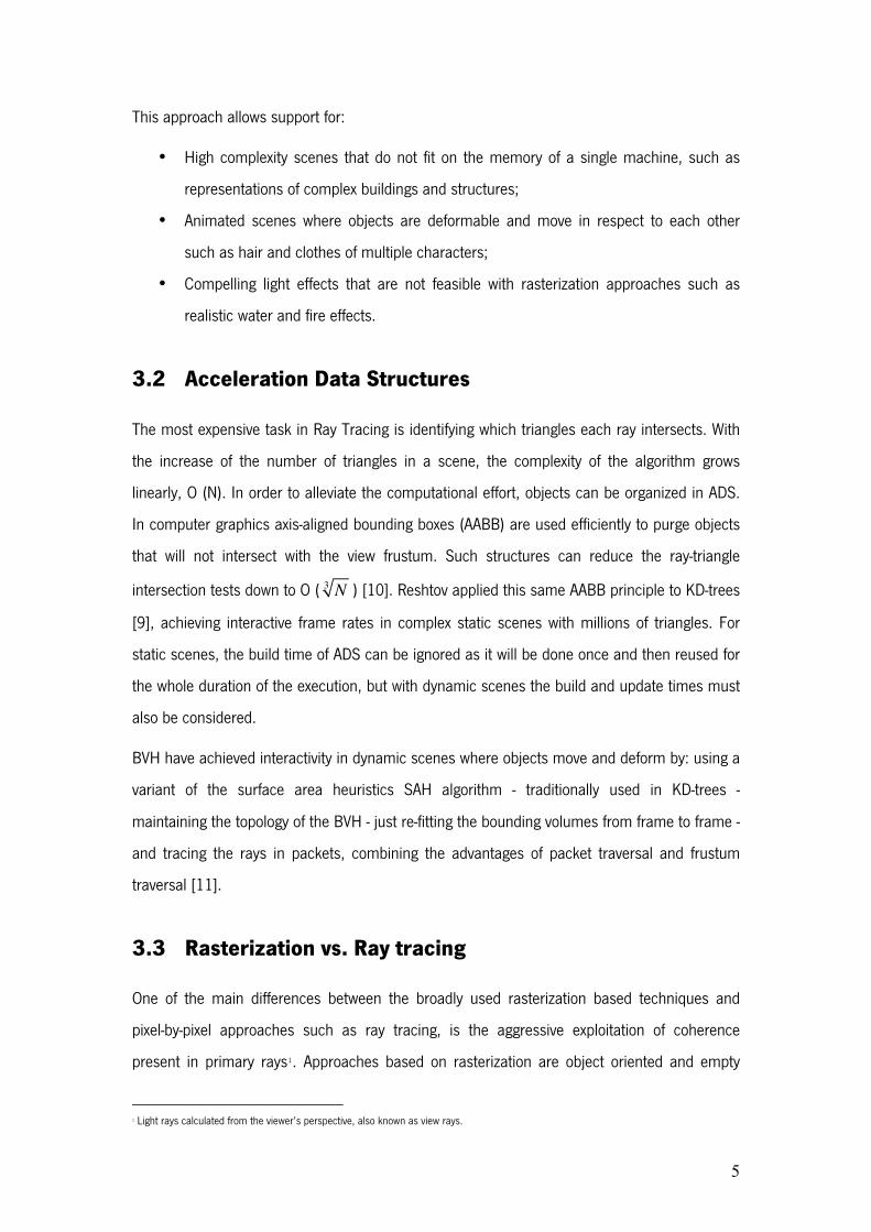
their neighbourhood. This is demonstrated in Figure 1, depicting how the rays that originate
from the same image region often represent the same objects or objects that are close in the
3D space of the scene. This assumption is also true for shadow regions that are often created
by the same object or objects that are close together.
2 In 1604, the German astronomer Johannes Kepler published “Astronomia pars Optica”, enunciating as principle that light rays travel from an object to the eye and not the other way around. 3 A shadow can be divided in two main parts: the umbra and the penumbra (there is also antumbra but usually it has no relevance in computer graphics). Umbra, known as hard shadow, can be described as the darkest part of the shadow, corresponding to areas fully occluded from a given light source and represented as black. Penumbra, known as soft shadow, is partially occluded regarding a given light and is represented by variable scales of darkness. Although hard shadows seldom produce a realistic shadow, they are considerably cheaper to generate than soft shadows. At the time of writing for this thesis, soft shadows were not implemented and we consider “shadows” as hard shadows.

7
Figure 1 - Light Path in Ray Tracing
Ray-tracers traditionally traversed the image plan in a scan line order. The scan line traversal
sequence breaks the ray coherence at the end of each line. As this approach only explores one
dimension then it might not be the most efficient method. As shadow rays are generated from
primary rays, the order by which primary rays are generated directly affects the order by which
shadow rays are processed. Spatial coherence and the impact of the traversal algorithm are
further explained in section 3.9.
Just for low to median frequency reflection rays, because rays are shot “randomly” in a
hemisphere, coherence is not obvious and thus not trivial to explore. Common techniques
used to exploit rays coherence are based on aggregation techniques that group rays in a
packet or beam based on the principle that coherent rays will traverse similar paths of the ADS
and thrive to test them individually as late as possible, thus reducing the ADS traversal cost.
3.5 Processing Packets instead of Single Rays
Modern high performance ray tracers employ the spatial coherence approach to reduce
computational costs. Current systems can employ ray aggregation techniques, combining
several rays into a packet and/or frustum4. The first enunciation of this technique was given by
Wald et al, proposing to trace rays in bundles of four through a KD-tree and use of SIMD
instructions to process these rays in parallel [14].
Ray aggregation techniques provide advantages for operations such as memory accesses,
function calls and traversal computations. This technique permits the use of SIMD instructions
4 Frustum is the portion of a solid that lies between two parallel planes cutting it. In the context of this thesis it refers to the three dimensional region that is visible on the screen.
8
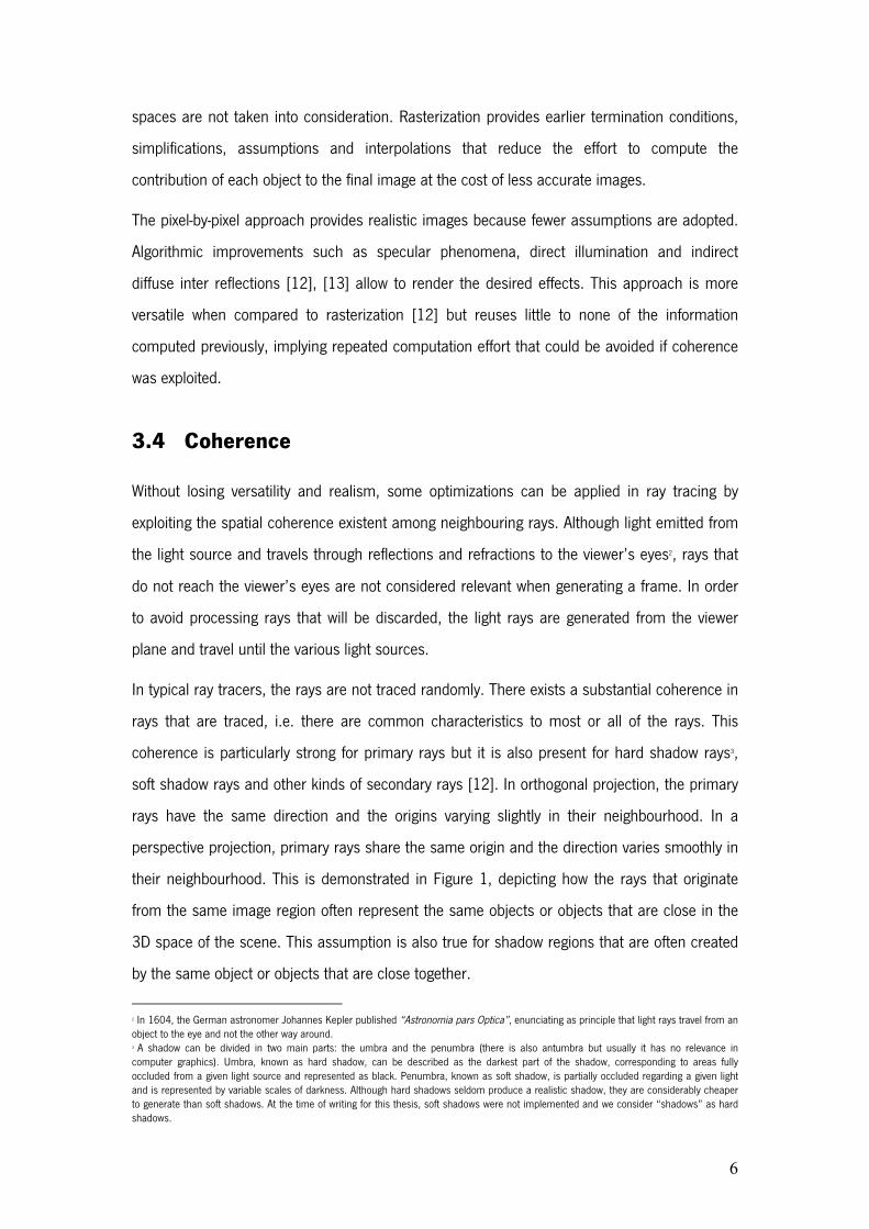
to gain greater performance from the CPU. Tracing rays with SIMD still requires performing the
traversal steps with SISD.
Nunes implemented a SIMD approach in iRT [13], using a packet of four rays, i.e. a set of four
floating point values and a four times speedup was expected as depicted on Figure 2.
However, the vectorial version is only capable of achieving speeds of 2.8 to 3.7 times faster
than the scalar version. Compared to the traditional scalar method, there exist no
disadvantages or limitations on this optimization other than the reordering of computation
tasks.
Figure 2 - SISD vs. SIMD
Dmitriev et al [15] proposed a broader concept of ray packing using frustum and interval
arithmetic-based techniques to avoid traversal steps or primitive intersections based on
conservative bounds of the packet of rays. Using the boundaries of the packets of rays, the
intersection of all the rays in the packet could be avoided if the full packet misses the triangle.
Reshtov has recently shown that even better performance could be achieved by building a
customized frustum at each leaf cell to exclude currently inactive rays [16]. He applied this
concept to a KD-tree traversal and used an arithmetic process based on “inverse frustum
culling” to cull complete sub trees during the traversal. This concept was later extended to
grids and BVH’s, as all of these contexts are sub-cases of AABB [17]. Although additional
research is required for improving the less coherent rays, packets and frustum techniques are
currently the method of choice for obtaining real-time performance.

9
3.6 Parallel Ray Tracing
Ray tracing supports independence of ray paths, thus being possible to parallelize the
computation of its paths. Interactive ray tracing is often achieved by resort to multilevel
parallelism such as sampling strategies, exploitation of memory locations and rays coherence
[12], [18].
In 2006, Parker et al. stated that “Almost ten years after the first interactive ray tracer was
introduced on a massive super computer, the necessary compute power to solve the same
visualization problems will be available on a workstation sized system.” [7]. This fact was
based on the improvement of individual processing power in modern CPUs. Besides this
processing capability increase, Manta has also exploited the emergent tendency of
workstations with multiple cores, providing a modular highly scalable parallel pipeline and
adopting SIMD instructions for vectorial processors. This modular pipeline gives the entire
system additional flexibility as new modules can be easily added or altered without the need of
code refactoring. As depicted below in Figure 3, Manta’s pipeline describes the stages
necessary to render a single frame.
Figure [7] - Manta's Pipeline for asynchronous rendering
Exception made for the load balancer, this figure represents a normal single threaded ray
tracing pipeline. Although the load balancer is represented as single block, it should be
perceived as three separate steps. First, the inherently load balanced tasks such as the pixel
sampling or packets construction are scheduled, followed by the load imbalanced tasks such
as rendering a packet or image deployment (usually only done by a single thread). After these
10
two steps, all threads dynamically balance the remaining workload. This way all threads get
similar amounts of work and the idle time at the threads-barrier is substantially reduced. With
the adoption of this pipeline, the threads synchronization happens only once per frame at the
end of each rendering loop. However, this method introduces a one-frame latency between the
image being rendered and outputted. If the frame rate is higher than ten frames per second,
this latency will hardly be perceived. Actually the one-frame latency allows that synchronization
happens at a single barrier, substantially simplifying interactions with the scene. Interactions
such as camera movements or scene animations require image displacement and ADS
restructuring, if these changes would be taken into consideration within a frame generation
then the work effort could be loss due to call-backs or images that become incoherent.
Another important and interesting aspect of Manta’s implementation is the adopted data
structure known as wide ray packets. Besides being used to communicate between the
different modules, each packet contains basic ray information as well as certain properties
common to all rays in the packet, such common origin or normalized direction vector. Besides
maintaining some degree of coherence among the rays that allow special optimizations, this
structure is designed for vectorial calculation. SIMD instructions usually require a vertical data
layout. To avoid costly memory re-arrangement, these packets accommodate the data fields
vertically so they can be directly loaded in the SIMD registers and uses horizontal access
methods so a horizontal layout can also be assumed at the cost of a slight performance
penalty.
The size of these packets is not bounded to a specific machine’s SIMD width or load balancer
tile size. In the case of Manta, the size can vary up to a maximum of 64 rays, which was found
to achieve the best performance because the entire packet can fit in the L1 cache [7]. With a
variable packet size and careful design of the packet’s data layout, splitting into smaller
packets can be made so that coherence of each packet is kept.
The load balancer along with thread-bounded ray packets and the pipeline referred above by
Manta allows deploying as many threads as desired without the need of reprogramming,
scaling almost linearly up to 64 processing units (92%) and achieves 82% efficiency with 126
processors.5
5 Results obtained for the model “Boeing 777” with 350 million triangles in an Itanium2 SGI super computer.
11
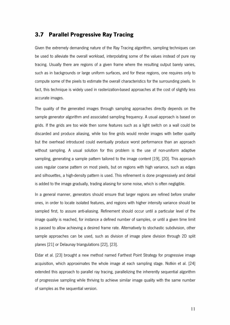
3.7 Parallel Progressive Ray Tracing
Given the extremely demanding nature of the Ray Tracing algorithm, sampling techniques can
be used to alleviate the overall workload, interpolating some of the values instead of pure ray
tracing. Usually there are regions of a given frame where the resulting output barely varies,
such as in backgrounds or large uniform surfaces, and for these regions, one requires only to
compute some of the pixels to estimate the overall characteristics for the surrounding pixels. In
fact, this technique is widely used in rasterization-based approaches at the cost of slightly less
accurate images.
The quality of the generated images through sampling approaches directly depends on the
sample generator algorithm and associated sampling frequency. A usual approach is based on
grids. If the grids are too wide then some features such as a light switch on a wall could be
discarded and produce aliasing, while too fine grids would render images with better quality
but the overhead introduced could eventually produce worst performance than an approach
without sampling. A usual solution for this problem is the use of non-uniform adaptive
sampling, generating a sample pattern tailored to the image content [19], [20]. This approach
uses regular coarse pattern on most pixels, but on regions with high variance, such as edges
and silhouettes, a high-density pattern is used. This refinement is done progressively and detail
is added to the image gradually, trading aliasing for some noise, which is often negligible.
In a general manner, generators should ensure that larger regions are refined before smaller
ones, in order to locate isolated features, and regions with higher intensity variance should be
sampled first, to assure anti-aliasing. Refinement should occur until a particular level of the
image quality is reached, for instance a defined number of samples, or until a given time limit
is passed to allow achieving a desired frame rate. Alternatively to stochastic subdivision, other
sample approaches can be used, such as division of image plane division through 2D split
planes [21] or Delaunay triangulations [22], [23].
Eldar et al. [23] brought a new method named Farthest Point Strategy for progressive image
acquisition, which approximates the whole image at each sampling stage. Notkin et al. [24]
extended this approach to parallel ray tracing, parallelizing the inherently sequential algorithm
of progressive sampling while thriving to achieve similar image quality with the same number
of samples as the sequential version.
12
Notkin et al. used a generator based on Elder’s Delaunay generator and defined tasks as a pair
of parameters: the image region, where tiles have a fixed size, and a number of samples, that
are variable. As a pre-processing stage, tasks are assigned in a round robin manner and a
local image complexity and variance is estimated in parallel by each processor. By multiplying
the estimated variance with the time the CPU took to complete the pre-processing stage, a
weight metric has been defined. Such weights are sent to the master node that thrives to
provide a uniform weight distribution that reassigns the tiles by the available processors. This
tile distribution will remain unchanged until the end of the frame.
After the pre-processing stage, new tasks are to be assigned dynamically using a Demand
Driven approach, gradually decreasing the task size to prevent big workloads in the last
samples of each frame6. Based on the principles mentioned above for a good sample generator
(large and/or big intensity variation regions should be refined first) the master thread assesses
a weight for every tile and assigns the slave threads to process the heavier tiles first. Once the
goal number of samples has been achieved then the results are collected by the master node,
which reconstructs the image.
For a 26-processor count, a speed up of 23.8 was achieved and registered a 15% of load
imbalance. Although not achieving a linear speed up, the quality achieved was extremely high
and had less than 5% of image resolution loss, which is barely perceivable. For this approach
to be tested the scenes were assumed to fit a single’s machine memory and this scenario is
not always true on parallel ray tracing systems.
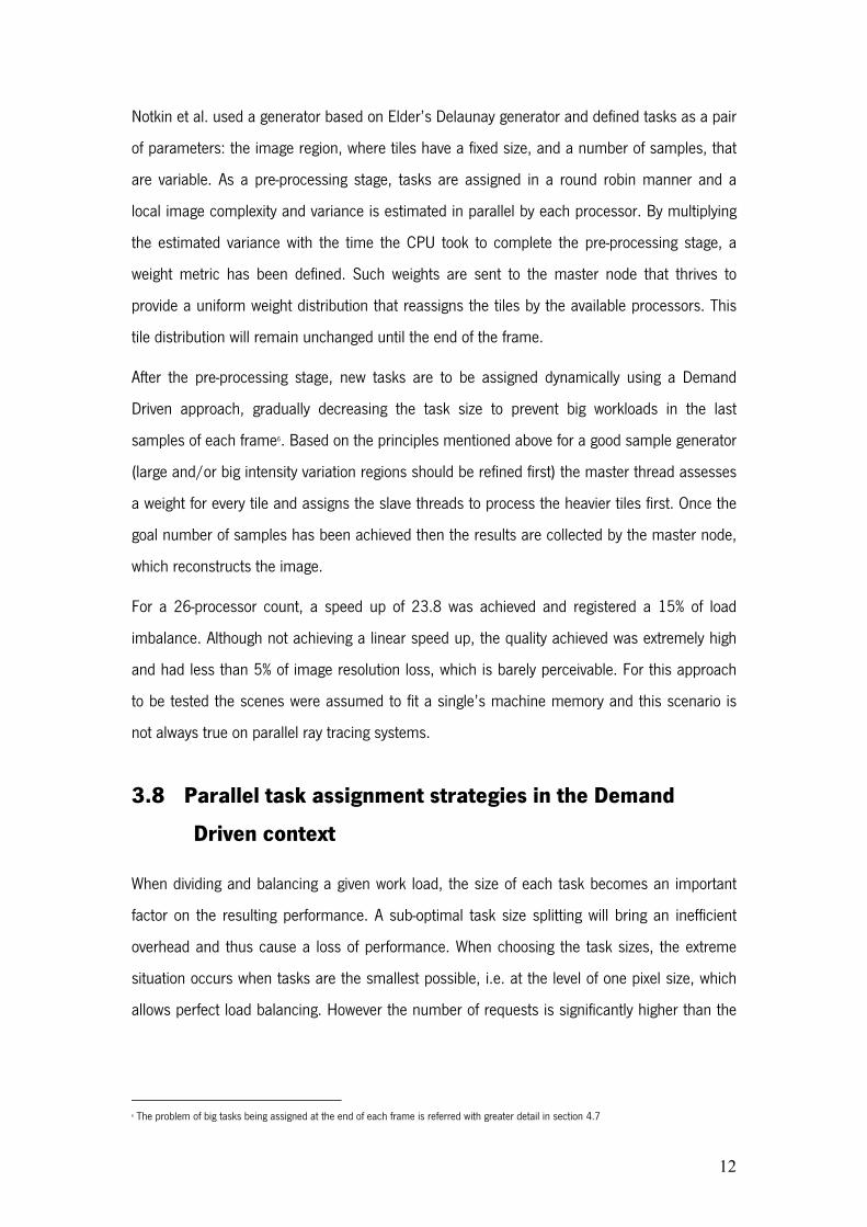
3.8 Parallel task assignment strategies in the Demand
Driven context
When dividing and balancing a given work load, the size of each task becomes an important
factor on the resulting performance. A sub-optimal task size splitting will bring an inefficient
overhead and thus cause a loss of performance. When choosing the task sizes, the extreme
situation occurs when tasks are the smallest possible, i.e. at the level of one pixel size, which
allows perfect load balancing. However the number of requests is significantly higher than the
6 The problem of big tasks being assigned at the end of each frame is referred with greater detail in section 4.7
13
workers and then leads to overheads such as latency7. On the other extreme there exist as
many tasks as workers, which results in minimal overhead but more prone to load imbalances.
In [25], Plachetka analyses how the task size can be determined based on the image space
sub-division and the number of available processors. Then, he proposes an anti-aliasing
approach with solutions for scenes that do not fit the available memory of each processor.
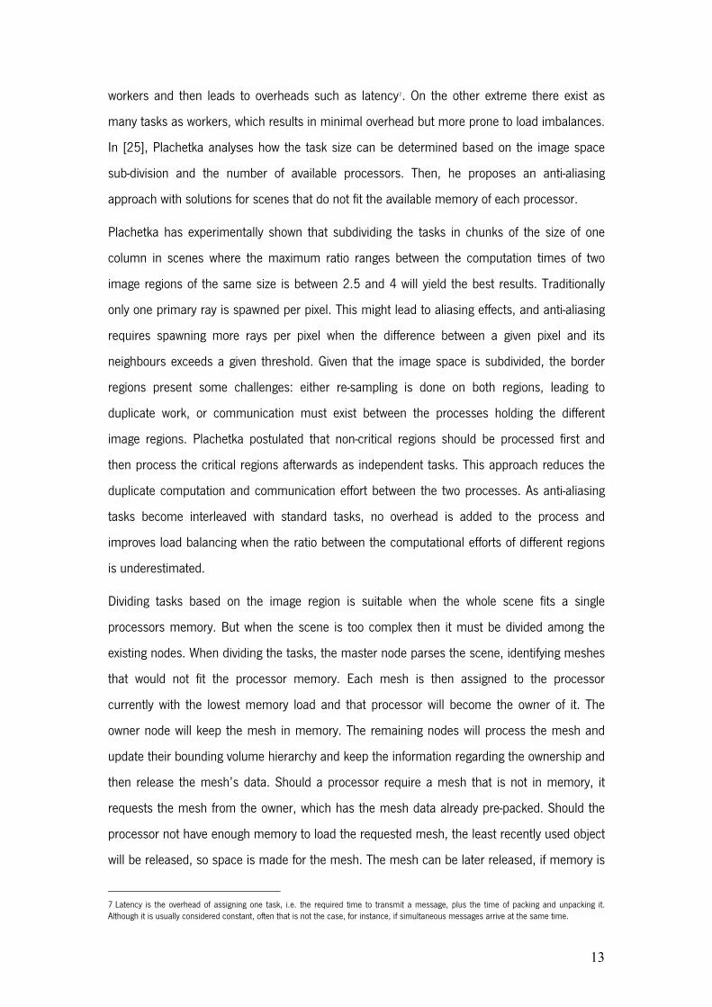
Plachetka has experimentally shown that subdividing the tasks in chunks of the size of one
column in scenes where the maximum ratio ranges between the computation times of two
image regions of the same size is between 2.5 and 4 will yield the best results. Traditionally
only one primary ray is spawned per pixel. This might lead to aliasing effects, and anti-aliasing
requires spawning more rays per pixel when the difference between a given pixel and its
neighbours exceeds a given threshold. Given that the image space is subdivided, the border
regions present some challenges: either re-sampling is done on both regions, leading to
duplicate work, or communication must exist between the processes holding the different
image regions. Plachetka postulated that non-critical regions should be processed first and
then process the critical regions afterwards as independent tasks. This approach reduces the
duplicate computation and communication effort between the two processes. As anti-aliasing
tasks become interleaved with standard tasks, no overhead is added to the process and
improves load balancing when the ratio between the computational efforts of different regions
is underestimated.
Dividing tasks based on the image region is suitable when the whole scene fits a single
processors memory. But when the scene is too complex then it must be divided among the
existing nodes. When dividing the tasks, the master node parses the scene, identifying meshes
that would not fit the processor memory. Each mesh is then assigned to the processor
currently with the lowest memory load and that processor will become the owner of it. The
owner node will keep the mesh in memory. The remaining nodes will process the mesh and
update their bounding volume hierarchy and keep the information regarding the ownership and
then release the mesh’s data. Should a processor require a mesh that is not in memory, it
requests the mesh from the owner, which has the mesh data already pre-packed. Should the
processor not have enough memory to load the requested mesh, the least recently used object
will be released, so space is made for the mesh. The mesh can be later released, if memory is
7 Latency is the overhead of assigning one task, i.e. the required time to transmit a message, plus the time of packing and unpacking it. Although it is usually considered constant, often that is not the case, for instance, if simultaneous messages arrive at the same time.

14
needed for other structures, but data that might later be required for other processes, such as
shading, is saved.
With his experiments he postulates that the referred approaches are scalable and bring higher
speed-ups. When comparing the approach without anti-aliasing against the anti-aliased
approach then performance begins only to decrease after 40 processors are active. As for the
objects in memory, the experiments shown that if at least 20% of the scene can be kept in
memory, then the algorithm keeps performing above average on a scalable manner. If the
available memory size reduces, requests for object data dramatically increases, significantly
decreasing the performance and scalability of the algorithm.
3.9 Ray coherence techniques
It has been previously described in section 3.5 that rays can be grouped in packets in order to
reduce the costs of traversing the ADS. The quality of these packets strongly depends on how
the rays are grouped. In order to better understand the existing level of coherence, individual
rays are studied rather than packets.
The coherence existing between the rays directly depends on the order under which they are
generated, which is traditionally done in a scan line traverse of the image plane. This approach
limits the exploration of coherence to a single dimension and inherently breaks the coherence
at the end of each line.
Considering that reloading an object or part of the ADS to higher levels of the memory
hierarchy has an associated cost, an ideal traversal sequence of the image plane would be one
that visits all the pixels in the entire area of each object before moving on to the next one,
allowing to explore coherence in two dimensions.
Knowledge of the projection area and position of an object beforehand can become too costly
and unfeasible to implement, especially if applied to the context of a real-time application.
For the purpose of this thesis, we define two assumptions:
• Information of the projection area and position are unavailable
• Traversal sequence is fixed rather than adaptive
Having these assumptions in consideration, it was defined that selection should be based
solely upon the shape of the image plane traversal line.
15
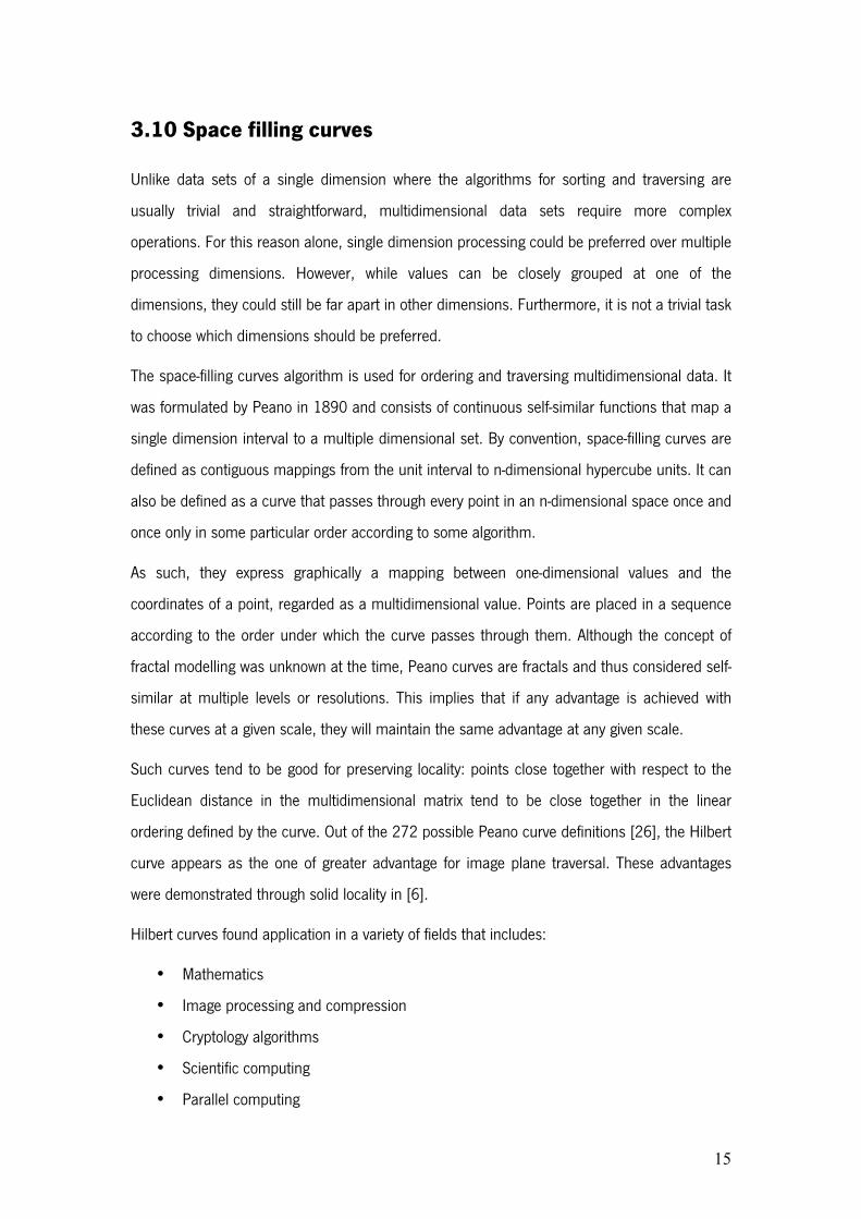
3.10 Space filling curves
Unlike data sets of a single dimension where the algorithms for sorting and traversing are
usually trivial and straightforward, multidimensional data sets require more complex
operations. For this reason alone, single dimension processing could be preferred over multiple
processing dimensions. However, while values can be closely grouped at one of the
dimensions, they could still be far apart in other dimensions. Furthermore, it is not a trivial task
to choose which dimensions should be preferred.
The space-filling curves algorithm is used for ordering and traversing multidimensional data. It
was formulated by Peano in 1890 and consists of continuous self-similar functions that map a
single dimension interval to a multiple dimensional set. By convention, space-filling curves are
defined as contiguous mappings from the unit interval to n-dimensional hypercube units. It can
also be defined as a curve that passes through every point in an n-dimensional space once and
once only in some particular order according to some algorithm.
As such, they express graphically a mapping between one-dimensional values and the
coordinates of a point, regarded as a multidimensional value. Points are placed in a sequence
according to the order under which the curve passes through them. Although the concept of
fractal modelling was unknown at the time, Peano curves are fractals and thus considered self-
similar at multiple levels or resolutions. This implies that if any advantage is achieved with
these curves at a given scale, they will maintain the same advantage at any given scale.
Such curves tend to be good for preserving locality: points close together with respect to the
Euclidean distance in the multidimensional matrix tend to be close together in the linear
ordering defined by the curve. Out of the 272 possible Peano curve definitions [26], the Hilbert
curve appears as the one of greater advantage for image plane traversal. These advantages
were demonstrated through solid locality in [6].
Hilbert curves found application in a variety of fields that includes:
• Mathematics
• Image processing and compression
• Cryptology algorithms
• Scientific computing
• Parallel computing
16
• Geographic information systems
• Database systems (to map multidimensional data to linearly ordered external memory
and to promote query efficiency)
• Distributed information systems (to partition multidimensional data in such way that
data sets that are close in Euclidean space are likely to be allocated to the same or
neighbouring processors).
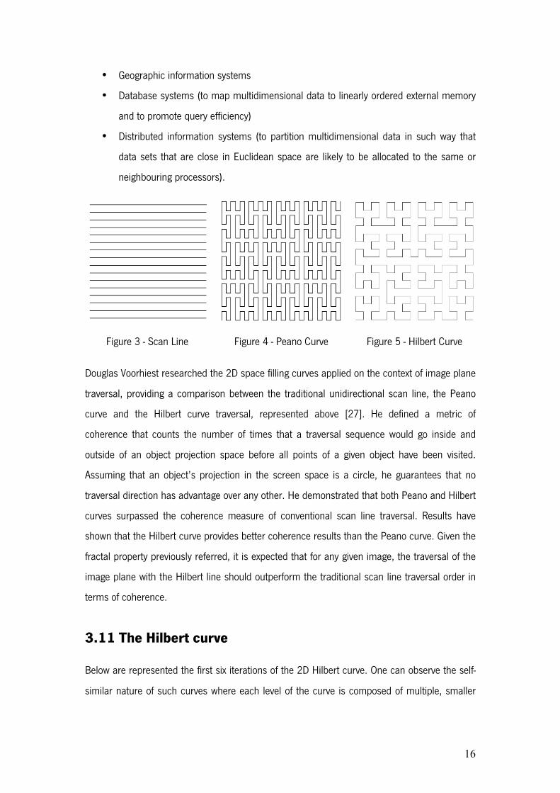
Figure 3 - Scan Line
Figure 4 - Peano Curve
Figure 5 - Hilbert Curve
Douglas Voorhiest researched the 2D space filling curves applied on the context of image plane
traversal, providing a comparison between the traditional unidirectional scan line, the Peano
curve and the Hilbert curve traversal, represented above [27]. He defined a metric of
coherence that counts the number of times that a traversal sequence would go inside and
outside of an object projection space before all points of a given object have been visited.
Assuming that an object’s projection in the screen space is a circle, he guarantees that no
traversal direction has advantage over any other. He demonstrated that both Peano and Hilbert
curves surpassed the coherence measure of conventional scan line traversal. Results have
shown that the Hilbert curve provides better coherence results than the Peano curve. Given the
fractal property previously referred, it is expected that for any given image, the traversal of the
image plane with the Hilbert line should outperform the traditional scan line traversal order in
terms of coherence.
3.11 The Hilbert curve
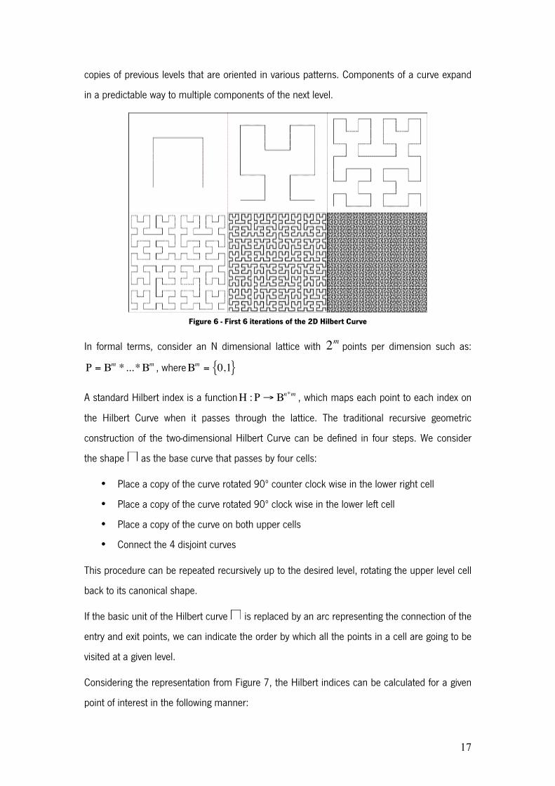
Below are represented the first six iterations of the 2D Hilbert curve. One can observe the self-
similar nature of such curves where each level of the curve is composed of multiple, smaller
17
copies of previous levels that are oriented in various patterns. Components of a curve expand
in a predictable way to multiple components of the next level.
Figure 6 - First 6 iterations of the 2D Hilbert Curve
In formal terms, consider an N dimensional lattice with 2m points per dimension such as:
Ρ = Βm *...*Βm , whereΒm = 0,1{ }
A standard Hilbert index is a functionΗ :Ρ → Βn*m , which maps each point to each index on
the Hilbert Curve when it passes through the lattice. The traditional recursive geometric
construction of the two-dimensional Hilbert Curve can be defined in four steps. We consider
the shape as the base curve that passes by four cells:
• Place a copy of the curve rotated 90º counter clock wise in the lower right cell
• Place a copy of the curve rotated 90º clock wise in the lower left cell
• Place a copy of the curve on both upper cells
• Connect the 4 disjoint curves
This procedure can be repeated recursively up to the desired level, rotating the upper level cell
back to its canonical shape.
If the basic unit of the Hilbert curve is replaced by an arc representing the connection of the
entry and exit points, we can indicate the order by which all the points in a cell are going to be
visited at a given level.
Considering the representation from Figure 7, the Hilbert indices can be calculated for a given
point of interest in the following manner:

18
a) Find the cell containing the point of interest, i.e. determining whether the point lies on
the upper or lower half plane regarding each dimension. Assuming we are working on
an order m curve, a point is represented by Ρ = p0, p1[ ]∈Βm *Βm . Determining
which half plane the point lies concerning the ith coordinate is equivalent to
determining the truth value of p < 2m−1 , which is equal to the m −1( )th bit of
pi,bit(pi,m −1)
b) Update key. Given the orientation at the current resolution (uniquely defined by the
entry e and exit f of the curve through the lattice), we can determine the order under
which each of the cells will be visited. Knowing that all points inside a cell are visited
before moving on to the next cell, the index of the focused cell will tell whether the
point of interest is visited in the first quarter of the curve or the second, and so on. In
other words, we may determine two bits of the Hilbert index h
c) Transform as necessary. Knowing the index i of the cell under which the point of
interest is located; we may determine the entry and exit points of the Hilbert curve
through this cell. The cell is then transformed with a rotation, (expressed as an
exclusive or), and reflected (expressed as a bitwise rotation operation) back into its
canonical orientation (entry in lower left, exit in lower right)
d) Continue until enough precision was attained. Zooming in at the cell containing our
point of interest, we can now inspect an order m - 1 Hilbert curve through a sub-cell of
our original space. We repeat this procedure for each of the remaining m - 1 levels of
precision, at each time calculating further 2 bits of the Hilbert index. At the end of the
process, we have a 2m bit Hilbert index, isolating a single point on the curve of length
22m through the Βm *Βm lattice.
This algorithm can also be extended to further dimensions [6].
Figure 7 - First four iterations of the 2D Hilbert curve in arc view

19
4 METODOLOGY
4.1 iRT Overview
The iRT is part of a broader project IGIDE. The main goal of IGIDE is to develop a physically
based global illumination renderer that is capable of generating accurate images at interactive
rates within dynamic time-varying virtual models. Users should be able to navigate and interact
within the virtual environment while visualizing perceptually accurate images that can be used
in a predictive manner.
As a starting version in March 2009, iRT is single threaded application that traces single rays
using work tasks in the form of rays or packets of rays, written onto a queue that feeds the
rendering process to output an image. iRT is tracing single rays (scalar code) or packets of four
rays (vectorized code based on SIMD extensions of the x86_64 architecture), using BVH as the
ADS to speed up the rendering time by reducing the number of ray-triangle intersections. The
rays processing pipeline is depicted in Figure 8 and further described in the paragraphs bellow.
Figure 8 - iRT Pipeline
A module called “Camera” represents the image plane and generates the primary rays and
adds them to a work queue. The ADS is then traversed to find the list of triangles belonging to
the voxels touched by the ray. The selected triangles are then intersected with the rays to
determine whether the rays actually intersect them or not and, in case they do, which are the
closest to the rays’ origin.
20
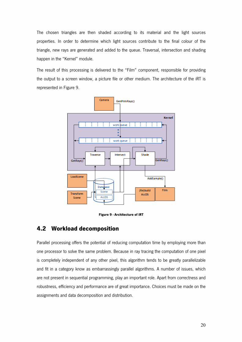
The chosen triangles are then shaded according to its material and the light sources
properties. In order to determine which light sources contribute to the final colour of the
triangle, new rays are generated and added to the queue. Traversal, intersection and shading
happen in the “Kernel” module.
The result of this processing is delivered to the “Film” component, responsible for providing
the output to a screen window, a picture file or other medium. The architecture of the iRT is
represented in Figure 9.
Figure 9 - Architecture of iRT
4.2 Workload decomposition
Parallel processing offers the potential of reducing computation time by employing more than
one processor to solve the same problem. Because in ray tracing the computation of one pixel
is completely independent of any other pixel, this algorithm tends to be greatly parallelizable
and fit in a category know as embarrassingly parallel algorithms. A number of issues, which
are not present in sequential programming, play an important role. Apart from correctness and
robustness, efficiency and performance are of great importance. Choices must be made on the
assignments and data decomposition and distribution.

21
In the context of ray tracing, decomposing the problem in independent tasks is the most
common approach. This exploits the inherently parallel nature of the algorithm, by subdividing
the image plane in smaller regions. With this approach, sequential algorithms can be easily
parallelized and improvements on the sequential algorithm can be directly applied on the
parallel approach. It also requires minimum communication between the processes, which
allows a centralized approach and offers high scalability. On the downside, this approach has
inherent issues with load balancing, as workload cannot be computed beforehand, scene must
be replicated in every processor and poses challenges for techniques that require data from
other regions, such as anti-aliasing.
Another approach, especially suited for big scenes, which do not fit in a single processors
memory, is the decomposition of the objects in the scene. With this approach scene sizes can
scale with the amount of processors, however, this requires complex designs and load
balancing becomes a difficult challenge to overcome.
Control-oriented approaches are less common but also present in ray tracing, mostly in
combination with one of the above. In this type of approaches, different processors are
responsible for different tasks, such as collision detection and shading. An example of this
approach being used together with image plane decomposition is given by Plachetka in [28],
also described in section 3.8, to solve the antialiasing problematic with image space
decomposition.
In the case of the ray tracer used within the context of this thesis, it was decided to use the
image decomposition approach, since the ray tracer is used with small and medium static
datasets, thus the scene can be easily replicated and there will be no repeated computation as
the scenes are static.
4.3 Measuring efficiency of parallelization
Let T1 be the execution time on 1 processor and Tn the execution time on n processors.
Speedup is given by S = T1Tn
, expressing how much the overall performance increased with the
increase of processing power, whereas efficiency (E ) is given by E = Sn=T1nTn
, measuring
the speedup gained with the increase of the computational power. This definition gives
22
efficiency E = 100% if increasing the number of processors p by a factor of n also
increases the speed by the same factor. That is tnp = ntp . When the efficiency is 100%, there
is a linear relationship between n and tnp , meaning that the efficiency is independent from
the number of processor and the speedup varies linearly with the number of processes.
If the efficiency can be held to near 100% then intuitively we feel we are getting a good return
for the extra cost of the extra processors. If the efficiency declines from 100%, we feel that we
are paying for more processors but we are not getting a proportional increase of speed.
4.4 Static Distribution
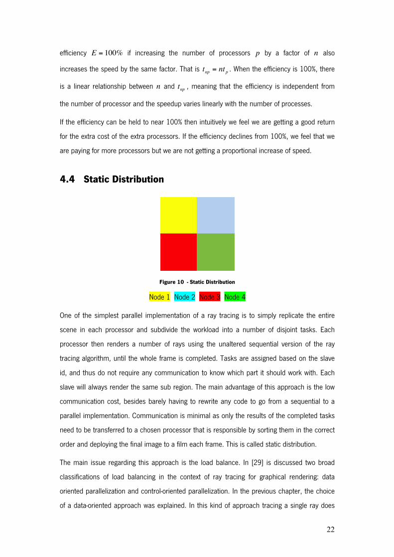
Figure 10 - Static Distribution
Node 1 Node 2 Node 3 Node 4
One of the simplest parallel implementation of a ray tracing is to simply replicate the entire
scene in each processor and subdivide the workload into a number of disjoint tasks. Each
processor then renders a number of rays using the unaltered sequential version of the ray
tracing algorithm, until the whole frame is completed. Tasks are assigned based on the slave
id, and thus do not require any communication to know which part it should work with. Each
slave will always render the same sub region. The main advantage of this approach is the low
communication cost, besides barely having to rewrite any code to go from a sequential to a
parallel implementation. Communication is minimal as only the results of the completed tasks
need to be transferred to a chosen processor that is responsible by sorting them in the correct
order and deploying the final image to a film each frame. This is called static distribution.
The main issue regarding this approach is the load balance. In [29] is discussed two broad
classifications of load balancing in the context of ray tracing for graphical rendering: data
oriented parallelization and control-oriented parallelization. In the previous chapter, the choice
of a data-oriented approach was explained. In this kind of approach tracing a single ray does

23
not seem to present great difficulties, but when it is done massively, it becomes an issue given
that each ray may generate unpredictable large tasks, by adding several new rays to the work
queue, while other rays leave the scene almost immediately after a single test. This generates
considerable differences in the workload of independent processors. This is mainly due to
diverse complexities of different sub regions of the image.
4.5 Static-Cyclic Distribution
When multiple computers operate in parallel to solve a single problem, some processors will
eventually be more heavily loaded than the others. As a result, some processors may have no
work left to do while others are still hardly working on the assigned task. Several methods of
load balancing to alleviate this problem have already been studied. Although it is usually not
possible to predict which subsets of rays will take the longest to trace, which makes it difficult
to avoid a load imbalance problem. A static approach to alleviate load imbalances can be
achieved by assigning multiple small regions for different areas of the image plane to each
processor, instead of a single sub region. This way, if a given sub region is more complex its
complexity will eventually be evenly distributed among all processors. The same is valid for
simpler sub regions.
Figure 11 - Static-Cyclic Distribution
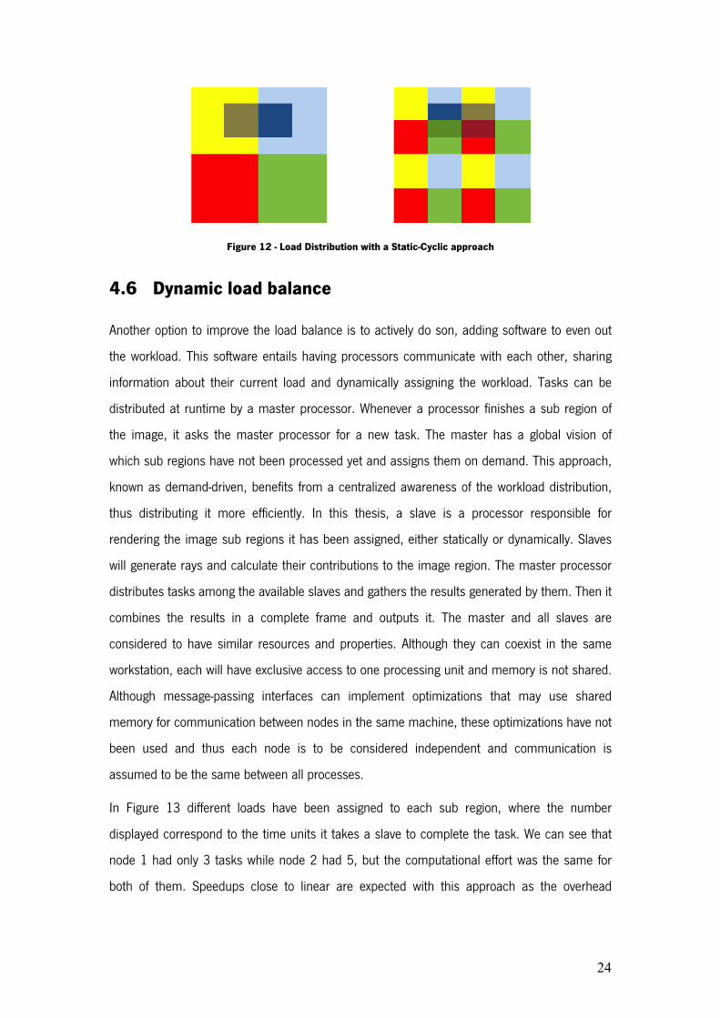
Consider the Figure 12, where the dark region represents a high load section. On the left we
see the standard case of static distribution of work. Only Nodes 1 and 2 process the heavy
load. On the right figure, we can see that by dividing the tasks in smaller chunks and assigning
them cyclically, distributes the critical region among all processes. This approach, called Static-
Cyclic, assigns tasks in a Round Robin fashion, a naïve approach to share critical regions
among all processors.
24
Figure 12 - Load Distribution with a Static-Cyclic approach
4.6 Dynamic load balance
Another option to improve the load balance is to actively do son, adding software to even out
the workload. This software entails having processors communicate with each other, sharing
information about their current load and dynamically assigning the workload. Tasks can be
distributed at runtime by a master processor. Whenever a processor finishes a sub region of
the image, it asks the master processor for a new task. The master has a global vision of
which sub regions have not been processed yet and assigns them on demand. This approach,
known as demand-driven, benefits from a centralized awareness of the workload distribution,
thus distributing it more efficiently. In this thesis, a slave is a processor responsible for
rendering the image sub regions it has been assigned, either statically or dynamically. Slaves
will generate rays and calculate their contributions to the image region. The master processor
distributes tasks among the available slaves and gathers the results generated by them. Then it
combines the results in a complete frame and outputs it. The master and all slaves are
considered to have similar resources and properties. Although they can coexist in the same
workstation, each will have exclusive access to one processing unit and memory is not shared.
Although message-passing interfaces can implement optimizations that may use shared
memory for communication between nodes in the same machine, these optimizations have not
been used and thus each node is to be considered independent and communication is
assumed to be the same between all processes.
In Figure 13 different loads have been assigned to each sub region, where the number
displayed correspond to the time units it takes a slave to complete the task. We can see that
node 1 had only 3 tasks while node 2 had 5, but the computational effort was the same for
both of them. Speedups close to linear are expected with this approach as the overhead

25
introduced is minimal. Communication is ought to be minimal, thus it is expected that a large
number of processors can be added before a bottleneck occurs.
Figure 13 - Dynamic Load Balancing
Two main types of communication are needed in this approach: task distribution and results
gathering. While the master node has tasks to be completed, it sends new tasks to the slaves
that are idle. The second happens when the slave finished computing the results and sends its
contribution back to the master. When the rendering of a frame starts, the master knows that
every slave is free, and once a task has been sent, the master considers that the slave is busy.
When a slave returns its results, the master knows that it is free again and can send more
tasks. The master does the generation of the final frame gradually, every time it receives new
results.
Three major issues were identified with this approach:
• At the beginning of each frame, slaves are idle until a new task is received. To
overcome this, each slave will autonomously pick a given sub region, based on its id.
Once the first task is complete, the results are sent to the master, that replies with the
next task.
• A slave is idle between finishing a task and receiving a new one. To mitigate this idle
time, each slave can be assigned more multiple tasks. If the master is expected to be
highly loaded, more tasks can be assigned to each slave. This reduces the chances of
the slaves being idle, but increases the likelihood of load imbalances. If the master is
considered to be lightly loaded, just one task needs to be assigned to mitigate this
problem. The ray tracer implemented in this thesis has just one task buffer.
• When distributing the last tasks of a frame, there is no room for load balancing, as no
more tasks can be assigned to idle processors. Although this cannot be avoided, it can
be mitigated by gradually refining the tasks size.
26
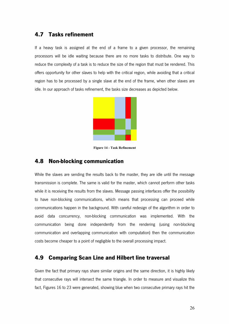
4.7 Tasks refinement
If a heavy task is assigned at the end of a frame to a given processor, the remaining
processors will be idle waiting because there are no more tasks to distribute. One way to
reduce the complexity of a task is to reduce the size of the region that must be rendered. This
offers opportunity for other slaves to help with the critical region, while avoiding that a critical
region has to be processed by a single slave at the end of the frame, when other slaves are
idle. In our approach of tasks refinement, the tasks size decreases as depicted below.
Figure 14 - Task Refinement
4.8 Non-blocking communication
While the slaves are sending the results back to the master, they are idle until the message
transmission is complete. The same is valid for the master, which cannot perform other tasks
while it is receiving the results from the slaves. Message passing interfaces offer the possibility
to have non-blocking communications, which means that processing can proceed while
communications happen in the background. With careful redesign of the algorithm in order to
avoid data concurrency, non-blocking communication was implemented. With the
communication being done independently from the rendering (using non-blocking
communication and overlapping communication with computation) then the communication
costs become cheaper to a point of negligible to the overall processing impact.
4.9 Comparing Scan Line and Hilbert line traversal
Given the fact that primary rays share similar origins and the same direction, it is highly likely
that consecutive rays will intersect the same triangle. In order to measure and visualize this
fact, Figures 16 to 23 were generated, showing blue when two consecutive primary rays hit the

27
same triangle and black otherwise. This test was run both with a scan line and with a Hilbert
curve traversal of the image plane.
Figure 15 - Bunny - Scan Line
Figure 16 - Bunny - Hilbert Curve
Figure 17 - Office - Scan Line
Figure 18 - Office - Hilbert Curve
Figure 19 - Sibenik - Scan Line
Figure 20 - Sibenik - Hilbert Curve

28
Figure 21 - Sponza - Scan Line
Figure 22 - Sponza - Hilbert Curve
The first thing that can be observed in the pictures is that there is a huge amount of coherence
to be exploited. Most part of the pictures is blue, indicating us that repeated work exists, which
can possibly be avoided. The following table shows the absolute count of blue dots for the
studied scenes with the two proposed approaches. The results shown are for a resolution of
256 x 256 pixels, thus the total pixel count is 65 536.
Table 1 - Coherence in Primary Rays
Results Bunny Conference Sibenik Office Sponza
Scan line 61662 53836 38427 59392 44016
Hilbert Line 61590 54168 40817 58335 45645
Coherence8 94% 83% 62% 89% 70%
Gain9 0.0% 0.1% 0.6% -0.2% 0.4%
This confirms that there is actually great coherence in the traversal order of the screen plane,
but shows us little advantage of the Hilbert line over the scan line, being sometimes even
worst. Although this showed no promises of better exploitation of coherence with Hilbert lines,
optimizations were designed and implemented given that so much coherence is available in
the primary rays. The most costly part in ray tracing is traversing the ADS10, where several tests
8 Coherence(%) = Max(Scanline,Hilbert) *100
Tpixels
9 Gain(%) = Hilbert *100
Scanline−100
10 A BVH is used in this example but the same technique can be applied to other ADS such as KD-trees

29
have to be made to find all the triangles that a ray intersects. It is then necessary to determine
which of the triangles is the closest to the ray origin (all the others will be occluded by the first
one and thus will not contribute to the current ray). In the ray tracer used in this thesis, finding
the closest triangle to the ray source was done in two steps: first determining the list of
triangles intersected by the ray and then identifying which one is closer. Both steps were
combined in a single one, since once the ray hits a triangle, the maximum distance a triangle
is worth being tested is known, given that any other triangle that is farther will certainly be
occluded. Following this principle, any AABB of which the nearest plane, regarding the ray’s
origin, is further than an already intersected triangle can be safely ignored, since any triangle
the ray might intersect will certainly be farther. This optimization, referred as PET (Primary
Early Termination), can greatly reduce the overall number of traversal steps. As stated before
in section 3.4, two consecutive rays share similar origins and the same directions; therefore it
is highly likely that they intersect the same triangle. Thus a new ray could be intersected with
the closest triangle of the previous ray. If the new ray also intersects the same triangle we can
start the ADS traversal with a PET condition, thus reducing even more the necessary traversal
steps, with the small cost of storing the closest triangle and intersecting it with the new ray at
the beginning of the ADS traversal of the next ray.
“The power of classical ray tracing comes from the fact that the illumination signal is
computed anew for each shading point. The direct light sources are stratified and sampled,
and the indirect environment is sampled (or approximated from prior evaluations). This means
that the method can capture sharp shadows; when a point no longer sees a source, it falls
automatically into shadow, and if the source is sufficiently small, the shadow will be sharp.
Specular reflections and refractions are also easily captured, since the proper illumination
directions are evaluated when needed. All of these components of the illumination signal may
be refined adaptively to any level of precision and confidence.” [30].
With this in mind, a similar approach to PET can be applied to hard shadow rays, with a
significant difference: a shadow ray is generated for each light source, thus the triangle is kept
for each light source. For each shadow ray targeting a given light source, it is first tested
against the stored triangle (no test is made if the last shadow ray hit the light source). If
successful, the ADS is not traversed, as an occlusion has already been found. This
optimization is referred as OCC (Occlusion Culling). Given that the order primary rays are

30
processed determines the order secondary rays are generated, the traversal order of the image
plane directly influences the efficiency of this approach.
One last optimization used is called SET (Shadow Early Termination). In the case of shadow
rays, it is sufficient to know if the origin of the ray is occluded or not, i.e. if the shadow ray hits
any triangle. If so, the traversal of the ADS can be stopped as soon as a collision is found. This
approach has two advantages: first, it prevents unnecessary traversal steps of the ADS.
Second, the triangle with which the ray collided, and that is going to be used by the OCC, is
not necessarily the closest to the ray origin. The triangle size and orientation can vary, but
assuming that they have the same size and orientation, the further they are from the shadow
rays origin, and thus closer to the light source, the bigger the chance that it will occlude more
rays coming from nearby sources. This directly benefits the efficiency of the OCC algorithm.
31
5 RESULTS
5.1 Experimental Setup
The following tests were performed in the Search Cluster at University of Minho11. They were
performed in a cluster with 8 Quad-Core Xeon E5130 with 4 GB of Ram, connected with a
10Gbps Myrinet network. All the results presented are the median value of 10 executions.
5.2 Load Balancing
In tables 2 to 5 we can see the results of applying the different load balancing approaches to
the different scenes.
11 More information in http://search.di.uminho.pt/

32
Table 2 - Load Balancing – Bunnies
Results
(FPS/Efficiency12)
1 Slave 2 Slaves 4 Slaves 16 Slaves 32 Slaves
1: Static 1,0444
N/A
1,6438
78,6946%
2,879
68,9153%
11,086
66,3429%
20,1752
60,3683%
2: Static-Cyclic 1,0406
N/A
1,9204
92,275%
3,8353
92,144%
14,4389
86,7261%
27,9661
83,9882%
3: Dynamic 1,0482
N/A
2,0324
96,9497%
4,0213
95,9113%
15,4969
92,4054%
27,78
82,8236%
4: 3 + Overlap of
Comp. w/ Comm.
1,0444
N/A
2,0848
99,8064%
4,1741
99,9154%
16,9526
101,4496%
32,6008
97,5468%
5: 4 + Non-Blocking
Comm.
1,0494
N/A
2,0861
99,3921%
4,2178
100,4795%
17,0632
101,625%
32,9571
98,1431%
6: 5 + Task
refinement
1,0502
N/A
2,0851
99,2751%
4,1857
99,644%
17,1271
101,9335%
31,6754
94,2595%
12 Efficiency described in section 4.3
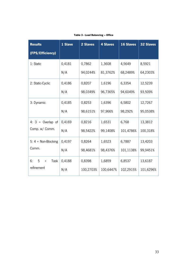
33
Table 3 - Load Balancing – Office
Results
(FPS/Efficiency)
1 Slave 2 Slaves 4 Slaves 16 Slaves 32 Slaves
1: Static 0,4181
N/A
0,7862
94,0244%
1,3608
81,3762%
4,5649
68,2489%
8,5921
64,2303%
2: Static-Cyclic 0,4186
N/A
0,8207
98,0349%
1,6196
96,7365%
6,3354
94,6049%
12,5239
93,509%
3: Dynamic 0,4185
N/A
0,8253
98,6151%
1,6396
97,966%
6,5802
98,292%
12,7267
95,0538%
4: 3 + Overlap of
Comp. w/ Comm.
0,4169
N/A
0,8216
98,5422%
1,6531
99,1408%
6,768
101,4786%
13,3812
100,318%
5: 4 + Non-Blocking
Comm.
0,4197
N/A
0,8264
98,4681%
1,6523
98,4376%
6,7887
101,1138%
13,4203
99,9451%
6: 5 + Task
refinement
0,4188
N/A
0,8398
100,2703%
1,6859
100,6447%
6,8537
102,2915%
13,6187
101,6296%
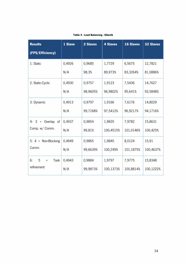
34
Table 4 - Load Balancing - Sibenik
Results
(FPS/Efficiency)
1 Slave 2 Slaves 4 Slaves 16 Slaves 32 Slaves
1: Static 0,4926
N/A
0,9685
98,3%
1,7729
89,973%
6,5675
83,3264%
12,7821
81,0886%
2: Static-Cyclic 0,4930
N/A
0,9757
98,9605%
1,9123
96,9802%
7,5436
95,641%
14,7627
93,5848%
3: Dynamic 0,4913
N/A
0,9797
99,7168%
1,9166
97,5412%
7,6176
96,9217%
14,8029
94,1716%
4: 3 + Overlap of
Comp. w/ Comm.
0,4937
N/A
0,9854
99,81%
1,9835
100,4515%
7,9782
101,0146%
15,8631
100,425%
5: 4 + Non-Blocking
Comm.
0,4949
N/A
0,9865
99,6639%
1,9845
100,249%
8,0124
101,1875%
15,91
100,4637%
6: 5 + Task
refinement
0,4943
N/A
0,9884
99,9873%
1,9797
100,1373%
7,9775
100,8814%
15,8348
100,1222%

35
Table 5 - Load Balancing – Sponza
Results
(FPS/Efficiency)
1 Slave 2 Slaves 4 Slaves 16 Slaves 32 Slaves
1: Static 0,3960
N/A
0,7648
96,5671%
1,3287
83,8822%
4,9544
78,1978%
9,4552
74,6185%
2: Static-Cyclic 0,3981
N/A
0,7829
98,3203%
1,5664
98,3641%
6,1088
95,9054%
11,914
93,5236%
3: Dynamic 0,3978
N/A
0,7716
96,9986%
1,5216
95,6481%
6,0421
94,953%
11,562
90,8499%
4: 3 + Overlap of
Comp. w/ Comm.
0,3974
N/A
0,7838
98,6286%
1,5936
100,261%
6,4522
101,4898%
12,733
100,1418%
5: 4 + Non-Blocking
Comm.
0,3977
N/A
0,7905
99,389%
1,5961
100,337%
6,483
101,8884%
12,7882
100,492%
6: 5 + Task
refinement
0,3973
N/A
0,7949
100,0485%
1,592
100,1865%
6,503
102,312%
12,8608
101,1701%
It is clear that the Static approach holds the lowest performance, mainly due to load
imbalances. In can be observed that by just applying a cyclic distribution of tasks, an
improvement of 20% to 30% of the efficiency of the parallel algorithm. The results where the
efficiency raises above 100% can be explained with the overhead existing in running the ray
tracer with just one slave, where the communication overhead already exists. We can also
observe that in the case of the Bunny, the tasks-refinement held worst results than without it.
This is understandable given that the last tasks, the bottom right corner, are covered by a
single triangle. This gives no advantage to the approach and increases the overhead of the
algorithm, as a single triangle has to be processed by multiple processors.

36
5.3 Spatial Coherence
To understand how much coherence exists, a colour map was implemented, colouring the
image according to the number of light sources occluded by the same triangle in consecutive
rays. The following images show on the left side the results of the scan line order and on the
right side the results of the Hilbert line order for five scenes, in order of appearance: Bunny,
Conference, Sibenik, Office, Sponza.
The colours represent:
1 Light Source Occluded 2 Light Sources Occluded
3 Light Sources Occluded 4 Light Sources Occluded
5 Light Sources Occluded 6 Light Sources Occluded
7 Light Sources Occluded 8 or more Light Sources Occluded
Figure 23 - Bunny - Scan Line
Figure 24 - Bunny - Hilbert Curve
Figure 25 - Office - Scan Line
Figure 26 - Office - Hilbert Curve
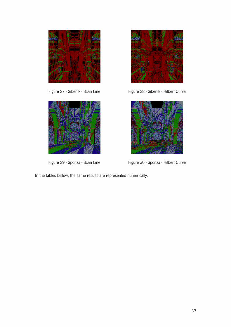
37
Figure 27 - Sibenik - Scan Line
Figure 28 - Sibenik - Hilbert Curve
Figure 29 - Sponza - Scan Line
Figure 30 - Sponza - Hilbert Curve
In the tables bellow, the same results are represented numerically.
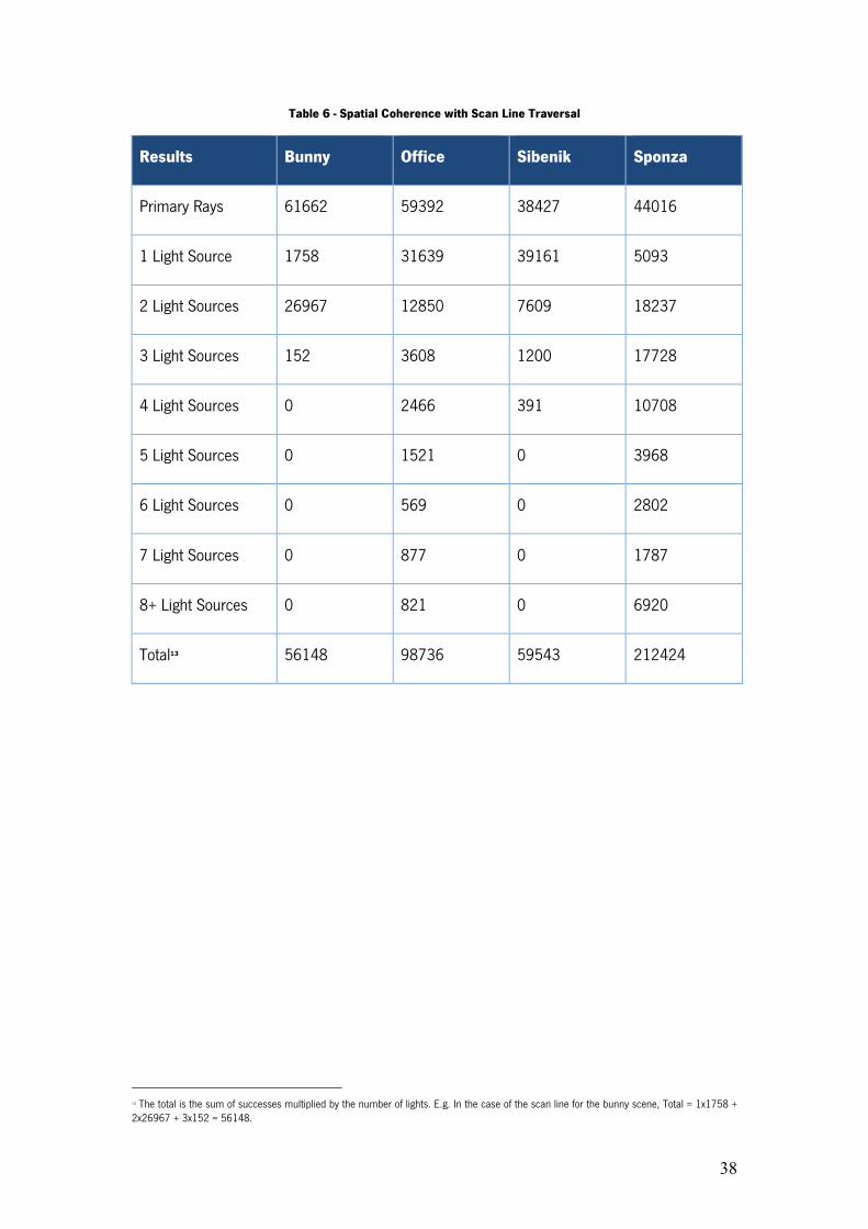
38
Table 6 - Spatial Coherence with Scan Line Traversal
Results Bunny Office Sibenik Sponza
Primary Rays 61662 59392 38427 44016
1 Light Source 1758 31639 39161 5093
2 Light Sources 26967 12850 7609 18237
3 Light Sources 152 3608 1200 17728
4 Light Sources 0 2466 391 10708
5 Light Sources 0 1521 0 3968
6 Light Sources 0 569 0 2802
7 Light Sources 0 877 0 1787
8+ Light Sources 0 821 0 6920
Total13 56148 98736 59543 212424
13 The total is the sum of successes multiplied by the number of lights. E.g. In the case of the scan line for the bunny scene, Total = 1x1758 + 2x26967 + 3x152 = 56148.

39
Table 7 - Spatial Coherence with Hilbert Curve Traversal
Results Bunny Office Sibenik Sponza
Primary Rays 61590 58335 40817 45645
1 Light Source 1725 32051 41049 5216
2 Light Sources 27061 12673 8552 16841
3 Light Sources 91 3607 1457 15888
4 Light Sources 0 1997 614 11134
5 Light Sources 0 1072 0 4827
6 Light Sources 0 429 0 3038
7 Light Sources 0 472 0 2077
8+ Light Sources 0 416 0 8385
Total 56120 89176 64980 220388
Table 8 shows the gain of the Hilbert Curve traversal in comparison to the Scan Line traversal.
The gain is calculated with the following formula:
Gain(%) = Hilbert *100Scanline
−100
Table 8 – Gain of Traversing the Image Plane with the Hilbert Curve against Scan Line
Results Bunny Office Sibenik Sponza
Primary Rays -0,1168 -1,7798 6,2196 3,701
These results show that although the approach changes the performance of the algorithm, it
does not conclude under which conditions each algorithm is better.

40
Below are the results of applying the above cited techniques for exploiting coherence, i.e., SET,
OCC and PET, for different scenes with different numbers of light sources.
Table 9 - Exploiting Coherence with Scan Line Traversal
Results
(FPS/Gain)
Bunny
3 LS
Office
8 LS
Sibenik
4 LS
Sponza
8 LS
Base 1,0444 0,4181 0,4926 0,3960
SET
1,2148
16,3142%
0,5158
23,3670%
0,5751
16,7463%
0,6226
57,2009%
OCC
1,2921
23,7161%
0,5572
33,2636%
0,6355
29,006%
0,6815
72,0758%
PET
1,0546
0,9686%
0,426
1,8851%
0,5441
10,4534%
0,4113
3,8540%
OCC-PET
1,3088
25,3155%
0,5741
37,2955%
0,7234
46,8477%
0,7294
84,1785%
SET-OCC-PET
1,3071
25,1467%
0,5745
37,4002%
0,7246
47,0925%
0,7307
84,5166%

41
Table 10 - Exploiting Coherence with Scan Line Traversal
Results
(FPS/Gain)
Bunny
3 LS
Office
8 LS
Sibenik
4 LS
Sponza
8 LS
Base 1,0413 0,4203 0,5091 0,3964
SET
1,2216
17,3103%
0,518
23,2305%
0,5943
16,7331%
0,6241
57,4298%
OCC
1,2891
23,7922%
0,5507
31,0216%
0,6763
32,8405%
0,7017
77,0081%
PET
1,0577
1,5705%
0,4285
1,9446%
0,5632
10,6246%
0,4132
4,2169%
OCC-PET
1,318
26,5638%
0,569
35,3643%
0,7881
54,7834%
0,7665
93,3401%
SET-OCC-PET
1,3137
26,1501%
0,5689
35,3384%
0,7883
54,8289%
0,7649
92,9385%
The results show that the spatial coherence present in the scene can be exploited. In fact
results have shown performance improvements of over 90% when many light sources are
present in the scene. The most successful approach exploiting coherence was the occlusion
culling. When combined with the PET approach, the improvements correspond to the
cumulative improvement of each algorithm, showing that they complement each other. As for
the SET approach, it seems to loose significance when the occlusion culling is also present.
This is expected as they both exploit the same feature, which is the fact that consecutive
shadow rays to a given light source are often occluded by the same triangle.

42
As for the difference between the scan line and the Hilbert curve traversals, the tests show that
there is no significant advantage of one over the other. This was already expected given the
results shown in Table 6.
The tested approaches might have not been the best, given that they only benefit two
consecutive rays, which is still a one-dimensional approach. Optimizations that would target a
given region, where the two dimensions influenced the efficiency of the approach, would
possibly benefit the Hilbert Curves.

43
6 CONCLUSIONS
6.1 Achieved goals
This study has shown that iRT could be successfully parallelized, achieving linear speed-ups,
as expected given the embarrassingly parallel nature of the algorithm. To achieve such speed-
ups, the resort to multiple techniques was necessary. Those include:
• Dynamic load balancing
• Efficient work load decomposition
• Adaptable tasks granularity
• Non-blocking communication
To the success of this approach much contributed the high performance of the network, that
kept the communication costs to a minimum and the efficiency of the Message Passing
Interfaces, that allowed to scale the application between different processors but also cores
within the same processor.
This studied also demonstrated the significant amount of coherence existent in the image
plane and how the image plane traversal order can change the efficiency of optimizations that
thrive on such spatial coherence. Strategies such as PET, OCC and SET improve the efficiency
of the algorithm, avoiding unnecessary computation, thus increasing the overall performance.
The amount of spatial coherence identified leaves the door open for other optimizations that
benefit from properties that are common to objects that appear near in the image plane.
6.2 Future work
Results have shown that the traversal algorithm has impact on the performance of the
proposed coherence optimizations, although it was not clear under which circumstances each
approach thrives. It is suggested as a future work that the strengths and weaknesses of each
approach are identified and exploited.

44
Although the optimizations designed and implemented work on a bi-dimensional plane, the
benefits are available only for two consecutive rays. Locality could be better exploited with
algorithms that cover an area, for instance an anti-aliasing algorithm. Such approaches could
potentially further benefit from the Hilbert curve traversal order.
45
7 BIBLIOGRAFY
[1] A. Oliveira, L. P. Santos, and A. Proença, “Refinement criteria for high fidelity interactive walkthroughs,” presented at the GRAPHITE '06: Proceedings of the 4th international conference on Computer graphics and interactive techniques in Australasia and Southeast Asia, 2006.
[2] T. Whitted, “An improved illumination model for shaded display,” Seminal graphics, Jul. 1998.
[3] M. J. Muuss, “Towards Real-Time Ray-Tracing of Combinatorial Solid Geometric Models,” Proceedings of BRL-CAD Symposium, pp. 1–15, Feb. 2008.
[4] Keates, “Interactive Ray Tracing on a Virtual Shared-Memory Parallel,” pp. 1–14, Nov. 2007.
[5] G. Peano, “Sur une courbe, qui remplit toute une aire plane,” Mathematische Annalen, vol. 36, no. 1, pp. 157–160, Mar. 1890.
[6] Hamilton, “Compact Hilbert indices: Space-filling curves for domains with unequal side lengths,” Inf Process Lett, vol. 105, no. 5, pp. 9–9, Feb. 2008.
[7] J. Bigler, A. Stephens, and S. G. Parker, “Design for Parallel Interactive Ray Tracing Systems,” Interactive Ray Tracing 2006, IEEE Symposium on, pp. 187–196, 2006.
[8] I. Wald, P. Slusallek, C. Benthin, and M. Wagner, “Interactive Rendering with Coherent Ray Tracing,” Computer Graphics Forum (Proceedings of EUROGRAPHICS), vol. 20, no. 3, pp. 153–164, 2001.
[9] A. Reshetov, “Multi-Level Ray Tracing Algorithm,” pp. 1–10, Sep. 2005.
[10] O. Karlík, “Utilization of generic programming in Ray Tracing,” 2009.
[11] I. Wald, S. Boulos, and P. Shirley, “Ray tracing deformable scenes using dynamic bounding volume hierarchies,” ACM Transactions on Graphics (TOG), vol. 26, no. 1, p. 6, 2007.
[12] I. Wald, W. R. Mark, J. Günther, S. Boulos, T. Ize, W. Hunt, S. G. Parker, and P. Shirley, “State of the Art in Ray Tracing Animated Scenes,” Eurographics 2007 State of the Art Reports, vol. 28, no. 6, pp. 1691–1722, 2009.
[13] M. Nunes, L.P. Santos, “Workload distribution for ray tracing in multi-core systems,” 2009.
[14] I. Wald, P. Slusallek, C. Benthin, and M. Wagner, “Interactive distributed ray tracing of highly complex models,” pp. 277–288, 2001.
[15] K. Dmitriev, V. Havran, and H.-P. Seidel, Faster Ray Tracing with SIMD Shaft Culling. 2004.
46
[16] A. Reshetov, “Faster Ray Packets - Triangle Intersection through Vertex Culling,” CORD Conference Proceedings, pp. 105–112, Sep. 2007.
[17] S. Boulos, I. Wald, and P. Shirley, “Geometric and arithmetic culling methods for entire ray packets,” University of Utah, 2006.
[18] I. Wald, C. P. Gribble, S. Boulos, and A. Kensler, “SIMD Ray Stream Tracing-SIMD Ray Traversal with Generalized Ray Packets and On-the-fly Re-Ordering,” SCI Institute, University of Utah, Technical Report# UUSCI-2007-012 (Aug. 2007), pp. 1–8, 2007.
[19] M. A. Z. Dippé and E. H. Wold, “Antialiasing through stochastic sampling,” presented at the SIGGRAPH '85: Proceedings of the 12th annual conference on Computer graphics and interactive techniques, 1985.
[20] D. P. Mitchell, “Generating antialiased images at low sampling densities,” vol. 21, no. 4, pp. 65–72, 1987.
[21] J. Painter and K. Sloan, “Antialiased ray tracing by adaptive progressive refinement,” vol. 23, no. 3, 1989.
[22] F. P. Preparata and M. I. Shamos, “Computational geometry: an introduction,” Computational geometry: an introduction, Sep. 1985.
[23] Y. Y. Eldar, M. M. Lindenbaum, M. M. Porat, and Y. Y. Y. Zeevi, “The farthest point strategy for progressive image sampling.,” IEEE Trans Image Process, vol. 6, no. 9, pp. 1305–1315, Dec. 1996.
[24] I. Notkin and C. Gotsman, “Parallel Progressive Ray-tracing,” vol. 16, no. 1, pp. 43–55, 1997.
[25] T. Plachetka, “Perfect load balancing for demand-driven parallel ray tracing,” Euro-Par 2002 Parallel Processing, pp. 91–120, 2002.
[26] “Space-filling curve,” Wikipedia.org. [Online]. Available: http://en.wikipedia.org/wiki/Space-filling_curve. [Accessed: 20-Oct.-2012].
[27] J. Arvo, “Graphics Gems II - James Arvo - Google Books,” 1991.
[28] T. Plachetka, “Tuning of algorithms for independent task placement in the context of demand-driven parallel ray tracing,” presented at the EG PGV'04: Proceedings of the 5th Eurographics conference on Parallel Graphics and Visualization, 2004.
[29] D. Badouel, K. Bouatouch, and T. Priol, “Distributing data and control for ray tracing in parallel,” Computer Graphics and Applications, IEEE, vol. 14, no. 4, pp. 69–77, 1994.
[30] A. S. Glassner, Principles of Digital Image Synthesis. 1995.
Top Related