


Línguas
Páginas
Legal


Department of EconomicsHow Much Does Investment Drive Economic Growth in China?
Duo Qin, Marie Anne Cagas, Pilipinas Quising and Xin-Hua He
Working Paper No. 545 August 2005 ISSN 1473-0278
How Much Does Investment Drive Economic Growth in China?
Duo QINa,b, *, Marie Anne CAGASb, Pilipinas QUISINGb, Xin-Hua HEc
a Economics Department, Queen Mary, University of London
b Economics & Research Department, Asian Development Bank c Institute of World Economics & Politics, Chinese Academy of Social Sciences
AUGUST 2005
ABSTRACT Investment-driven growth has long been regarded as a key development strategy in China. This
paper investigates empirically the validity of this view. Post-1990 data analyses and macro-
econometric model simulations show that market demand has become a regular force in driving
investment since reforms, that non-demand-driven investment growth contributes to increasing
capital-output ratio far more than output growth, that government investment exerts a pivotal role
in amplifying investment cycles, albeit effective in promoting employment, and that delayed and
rising consumption from current investment surge can help sustain the impact of growth even with
constant-returns-to-scale in the long-run GDP.
Key words: Investment, growth, impulse response function, cointegration, Granger non-causality JEL classifications: E22, E62, R34, O23, P41
* Contacting author; email: [email protected] .
1
By three methods we may learn wisdom: first, by reflection, which is noblest; second, imitation, which is easiest; and third by experience, which is the bitterest.
Confucius
I. Another East Asian ‘Miracle’?
The spectacular growth of China over the last two decades apparently adds significant
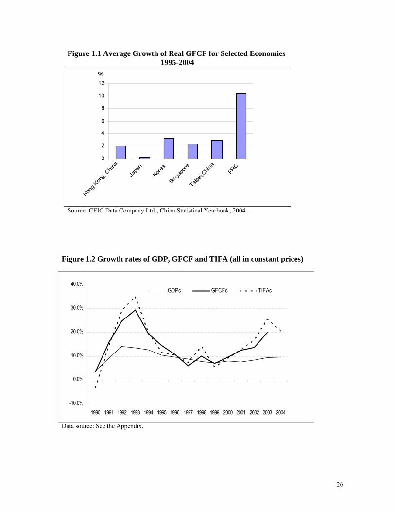
force to the East Asian ‘Miracle’.1 During the period 1990 – 2003, China’s growth has been
averaging 9.3% in terms of GDP per annum while the accompanying rate in gross fixed
capital formation (GFCF) is 14% and the rate of the total investment in fixed assets (TIFA)
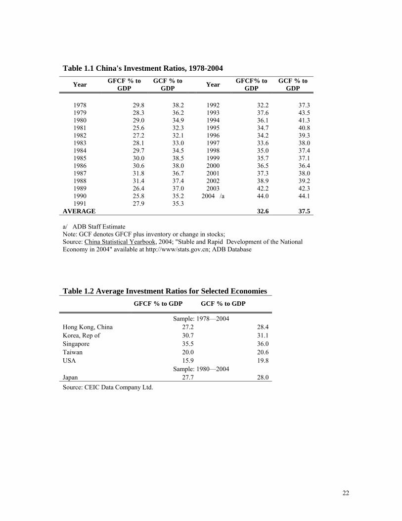
is 15%.2 Today, GFCF accounts for over 40% of nominal GDP, as compared to less than
30% in the early 1980s, see Table 1.1. These records have definitely outperformed those of
Japan and the US and many other Newly Industrialized Asian Economies (NIAEs), see
Table 1.2. The GFCF growth also remains high especially when compared with other Asian
economies, see Figure 1.1. In 2003 alone, GFCF recorded a growth of about 20% while
TIFA growth reached 25%.
In 2004, the startling acceleration of the TIFA – 43.2% growth in the 1st quarter and
33.3% in the 2nd quarter3 before settling down to 27.6% for the full year – has led the
Chinese government to curtail fixed assets investment out of the grave concern that the
rising investment would overheat the economy. The rapid investment expansion has caused
severe shortage in energy and raw material supplies, pushed imports to grow faster than
exports, and accelerated inflation. The investment price index rose to 5.6% and the
1 The East Asian ‘Miracle’ refers to the myth that the engine driving economic growth is essentially capital accumulation instead of total factor productivity growth, see e.g. (Young 1995) and (Senhadji 2000). 2 The TIFA is more often used than the GFCF in China, as it is published monthly and more timely than GFCF. Both GFCF and TIFA are deflated by the price index of fixed assets from the China Statistical Yearbook 2004 for the period 1991-2003. The price index of raw materials and energy is used for 1990 as the price index of fixed assets is unavailable that year. 3 All the statistics quoted are y-o-y rates.

2
consumer price index to 3.9% in 2004 as compared to 2.2% and 1.2% respectively in 2003.
However, GDP growth ended up at about the same level as 2003 in spite of the investment
fever and the tightening of investment policies.
The view that the Chinese economy is an investment-driven economy is a legacy from
the old regime of a centrally planned economy (CPE), e.g. see (Kornai 1980) for a general
theory of investment hunger of a CPE and see (Imai 1994) for an investment-led business
cycle model of China. And in spite of regime changes since the reforms, capital investment
has remained to be regarded as a vital factor to promote the economic growth, as
discernible from the recent literature. For example, Goldstein and Lardy (2004) anticipate
that it will take a few years for the Chinese economy to unwind the current investment
boom, possibly with a down turn, on the basis of the present investment curb. This
investment-driven growth view also finds support in a number of empirical studies, e.g. see
(Yu 1998), (Kwan et al 1999), and Zhang (2003).
However, the view that investment is the main engine of growth faces several
problems. Considering that the Chinese economy has undergone enormous changes since
the reform, can we find enough evidence to support the assertion that the old investment-
driven mechanism is still intact? If the Chinese economy has remained in an investment-led
track, why is it that the rate of GDP growth has always been significantly lower than the
rate of investment growth over the last 15 years?4 Why has the volatile investment cycles
not discernibly affected the GDP growth path, as shown from Figure 1.2? If one seeks
support of the view from levels rather than growth rates, how can we explain the visible
increasing GFCF/GDP ratio, as shown in Table 1.1? The increasing ratio actually suggests
4 By simple growth theory, output growth is only expected to be dampened by the capital input elasticity in comparison with the capital input growth, e.g. see (Rebelo 1991). Using the estimated elasticity of 0.8, 9.3% of GDP growth should only require 11.6% growth in capital.

3
that the Chinese economy is another East Asian ‘miracle’.5 If that is the case, how can we
reconcile the contradiction between the view of investment-driven growth and the
neoclassical growth theory, which states that accelerating capital accumulation alone
cannot sustain long-run economic growth in the absence of significant technical progress?
If we turn to new endogenous growth models for theoretical support, what are the
identifiable variables which would link investment to growth, (see George et al 2003)?
More fundamentally, one needs first to clearly define the investment-driven growth view as
the investment-output nexus is by no means a one-way causal relationship according to
endogenous growth theories.
The paper makes an empirical attempt to answer the above problems using post-1990
time-series data. We try to do this first by careful data analysis, see section 2. We then try
to assess empirically the magnitude and the manner by which investment drives economic
growth and vice versa. This we will do using a quarterly macro-econometric model of
China where both investment and GDP are endogenously determined, see Section 3.
Concluding remarks are in Section 4.
II. What do data tell us about the investment-GDP nexus?
In this section, we try to find answers to the questions posed in the previous section and
to examine all the possibly identifiable aspects of the investment-driven-growth view with
respect to aggregate investment and GDP data. Specifically, we to try to explain why
surges in investment have not been significantly transmitted into GDP surges — whether it
is investment growth or GDP growth which is dynamically leading the other, whether there
5 Evidence of overinvestment has also been presented in a number of recent publications, e.g. see (Zhang 2003), (Lin 2004) and (Wolf 2005).
4
exists simultaneous causality between the two aggregates in levels, and whether there has
been significant technological progress underlying the long-term growth.
Let us first try to answer the question why the investment surge has not been
significantly transmitted into GDP surge by analyzing the co-movement of the demand
components of GDP with respect to the GFCF changes. Denote real GDP by Y, real
consumption (including both private and government) by C, net exports by NX and
inventory (or change in stocks) by IS. The income identity can thus be presented as
NXISGFCFCY +++= .The corresponding growth equation is:
(1) 1t
1t
1t
1t
1t
1t
1t
1t
YIS.
ISY
NX.NX
YGFCF.
GFCFYC.
C.
Y−
−
−
−
−
−
−
− +++= .
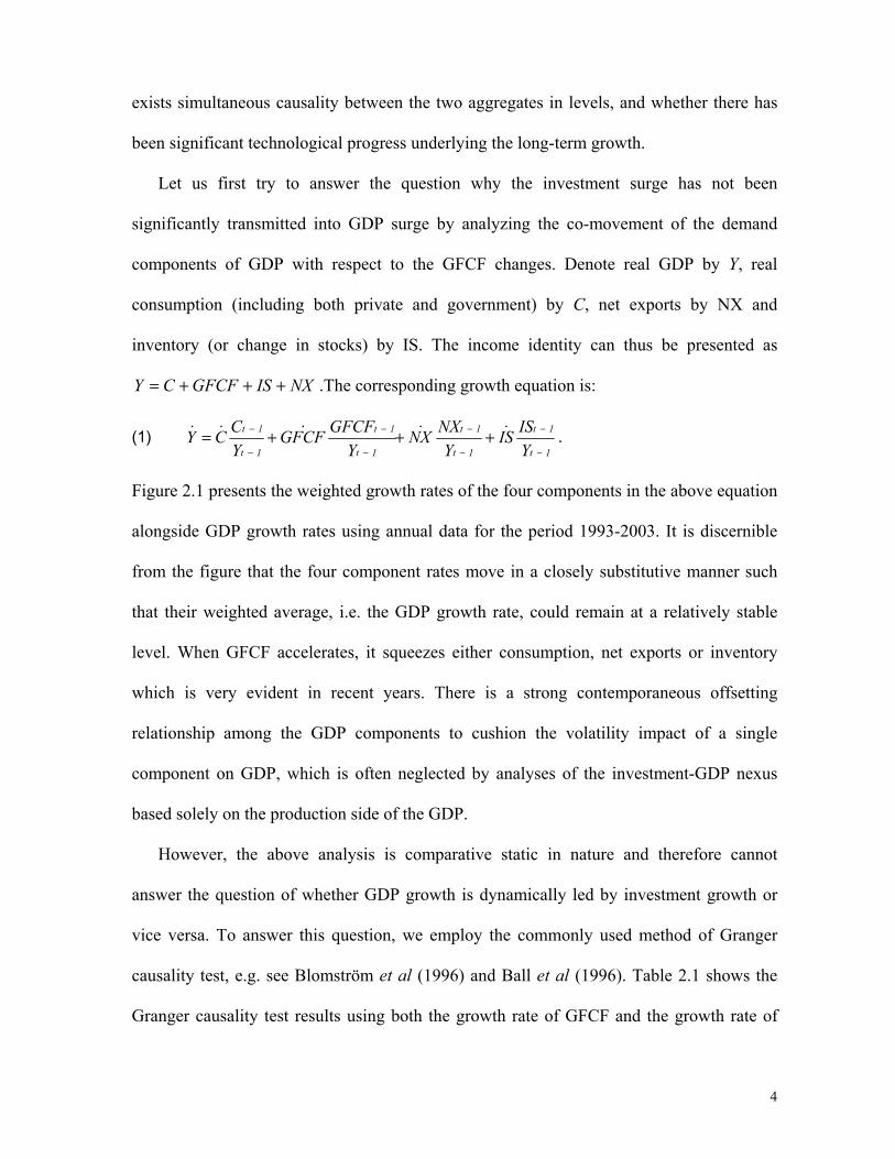
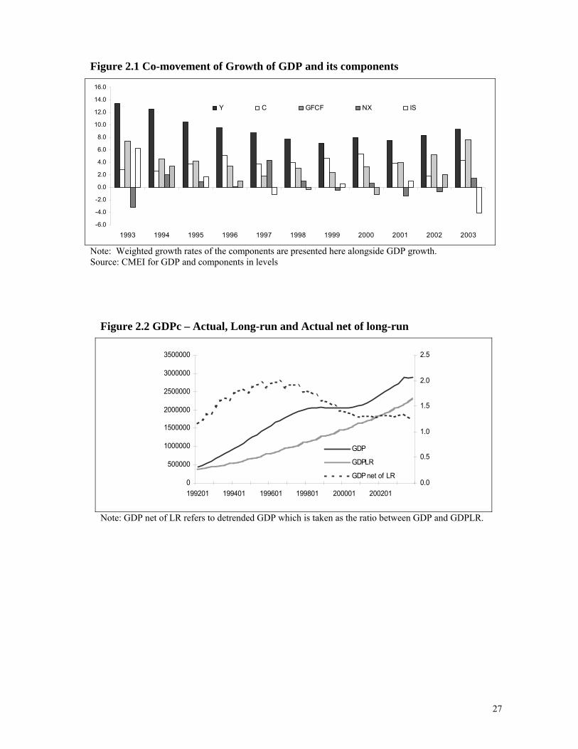
Figure 2.1 presents the weighted growth rates of the four components in the above equation
alongside GDP growth rates using annual data for the period 1993-2003. It is discernible
from the figure that the four component rates move in a closely substitutive manner such
that their weighted average, i.e. the GDP growth rate, could remain at a relatively stable
level. When GFCF accelerates, it squeezes either consumption, net exports or inventory
which is very evident in recent years. There is a strong contemporaneous offsetting
relationship among the GDP components to cushion the volatility impact of a single
component on GDP, which is often neglected by analyses of the investment-GDP nexus
based solely on the production side of the GDP.
However, the above analysis is comparative static in nature and therefore cannot
answer the question of whether GDP growth is dynamically led by investment growth or
vice versa. To answer this question, we employ the commonly used method of Granger
causality test, e.g. see Blomström et al (1996) and Ball et al (1996). Table 2.1 shows the
Granger causality test results using both the growth rate of GFCF and the growth rate of
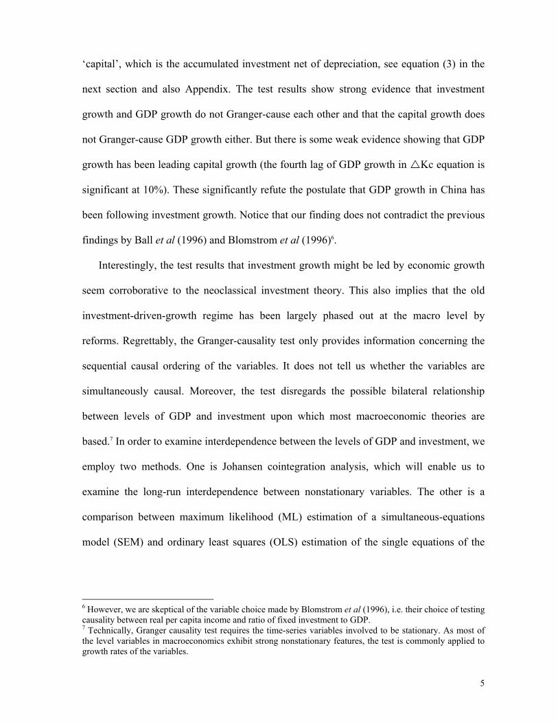
5
‘capital’, which is the accumulated investment net of depreciation, see equation (3) in the
next section and also Appendix. The test results show strong evidence that investment
growth and GDP growth do not Granger-cause each other and that the capital growth does
not Granger-cause GDP growth either. But there is some weak evidence showing that GDP
growth has been leading capital growth (the fourth lag of GDP growth in Kc equation is
significant at 10%). These significantly refute the postulate that GDP growth in China has
been following investment growth. Notice that our finding does not contradict the previous
findings by Ball et al (1996) and Blomstrom et al (1996)6.
Interestingly, the test results that investment growth might be led by economic growth
seem corroborative to the neoclassical investment theory. This also implies that the old
investment-driven-growth regime has been largely phased out at the macro level by
reforms. Regrettably, the Granger-causality test only provides information concerning the
sequential causal ordering of the variables. It does not tell us whether the variables are
simultaneously causal. Moreover, the test disregards the possible bilateral relationship
between levels of GDP and investment upon which most macroeconomic theories are
based.7 In order to examine interdependence between the levels of GDP and investment, we
employ two methods. One is Johansen cointegration analysis, which will enable us to
examine the long-run interdependence between nonstationary variables. The other is a
comparison between maximum likelihood (ML) estimation of a simultaneous-equations
model (SEM) and ordinary least squares (OLS) estimation of the single equations of the
6 However, we are skeptical of the variable choice made by Blomstrom et al (1996), i.e. their choice of testing causality between real per capita income and ratio of fixed investment to GDP. 7 Technically, Granger causality test requires the time-series variables involved to be stationary. As most of the level variables in macroeconomics exhibit strong nonstationary features, the test is commonly applied to growth rates of the variables.
6
model, which will enable us to examine contemporaneous interdependence, or simultaneity
as commonly called in econometrics.
Dickey-Fuller unit root test is carried out on GFCF, capital and GDP before Johansen
cointegration analysis is applied. There is fairly strong evidence showing that GDP and
GFCF are nonstationary I(1) variables from the test results (see Table 2.2). Being basically
accumulated investment, capital should be an I(2) variable. However, we find no adequate
evidence to show capital is I(2) rather than I(1). As unit root tests tend to have low power
when sample sizes are relatively small, we shall apply cointegration analysis on two pairs
of variables respectively, i.e. GDP versus GFCF and GDP versus capital, out of the
consideration that it is capital stock, rather than investment, which forms a key component
of aggregate production functions. It is evident from Table 2.3 that cointegration is not
rejected for either pair of variables. We can thus be fairly confident that GDP and GFCF, as
well as GDP and capital, are mutually interdependent in the long run, irrespective of the
difficulty in determining the exact degrees of nonstationarity of each variables involved.
Let us now examine whether the two pairs of variables are also contemporaneously
interdependent. A simple two-equation VAR (vector autoregression) system is set up for
this purpose. A SEM is then specified within the VAR and estimated first using ML
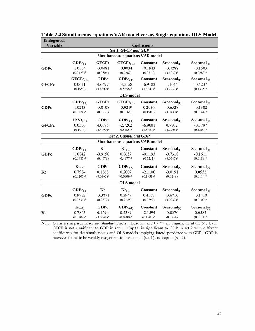
estimator and then single-equation OLS estimators. Table 2.4 reports the estimation results.
Set 1 in the table shows that GDP contemporaneously explains GFCF but not vice versa. In
other words, GDP appears to be weakly exogenous to GFCF. Set 2 on the other hand
indicates a fairly strong presence of simultaneity between capital and GDP (as ML
estimates are very different from OLS estimates). Interestingly, the simultaneity in the
GDP equation is essentially between GDP growth and capital growth which is roughly the
GFCF (i.e. the coefficient estimates support a growth model). The OLS estimates in the

7
capital equation of set 2 are statistically similar to those ML estimates, reinforcing the
above inference that GDP is weakly exogenous to capital or GFCF rather than vice versa.
These results enhance the inferences based on the Granger causality test, and provide
strong support to the claim that the Chinese economy is already out of the old investment-
led growth regime.
The view of investment-driven growth also faces the theoretical challenge that long-
term growth is independent of capital accumulation, unless there exist either increasing
returns to scale due to capital or technological progress. Empirical evidence shows that
increasing returns to capital is normally long-run untenable, see e.g. (Temple 1999). To
examine whether there has been significant technological progress underlying China’s
economic growth, we utilize the long-run GDP equation proposed by He and Qin (2004),
which assumes that the long-run GDP follow a simple Cobb-Douglas production function
with constant returns to scale. If there were significant technological progress, the actual
GDP de-trended by this long-run GDP should carry a visible upward trend. The actual
GDP, the long-run GDP and the de-trended GDP are plotted in Figure 2.2. Interestingly,
the de-trended GDP shows a slow cycle, with a significant downward movement since the
late 1990s, corresponding to the noticeable rise in the GFCF/GDP ratio as shown in Table
1.1. Thus, we do not reject the constant return to scale assumption — long-run economic
growth may not be dependent upon investment growth.
III. What does macroeconometric model tell us about the investment-GDP nexus?
The data evidence of the previous section shows that in comparative static terms, there
are counterbalancing demand factors that offset the impact of investment volatility on
GDP; that, in the long run, there has not been discernable trend of long-lasting
technological progress to reject the constant return to scale condition; and that there is
8
fairly strong evidence of simultaneity between investment and GDP although the causal
direction in terms of growth rates is more of GDP → investment than vice versa. However,
examination of data alone is inadequate for us to synthesize the above results and to
evaluate how much and in what way investment drives GDP growth both in the short run
and in the long run. To achieve these, one has to resort to the use of macro models.
A common type of macro model for this purpose is the endogenous or semi-
endogenous growth model, see (George et al 2003) for a recent survey and (Li 2000) for
semi-endogenous growth models. However, most of these models are still too theoretical
and too abstract to enable sound empirical inferences. For example, Agénor (2000, Chapter
13) points out how growth models are plagued by methodological problems in applications;
Temple (2003) warns applied economists against taking growth models too literally.
Therefore, we choose to use a full-fledged macro-econometric model of China as it is more
comprehensive and closer to the Chinese economy than any growth-theory based structural
models. The China model is a quarterly model built by the Economics and Research
Department of Asian Development Bank jointly with the Institute of World Economics and
Politics of the Chinese Academy of Social Sciences. The model contains 75 endogenous
variables and 16 non-modeled variables. It is estimated based on a data sample starting
from 1992Q1, see (He et al 2004) and (Qin et al 2005) for more detailed description of the
model and our modeling strategy.
As the investment-GDP nexus is the present focus, this entails a brief description of the
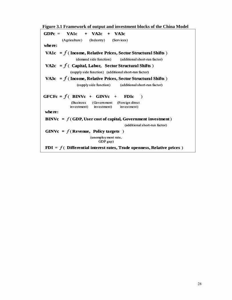
investment block and the output block of the model.8 There are four key equations in this
8 The basic structure of the investment block is first reported in He and Qin (2004). However, the block has been substantially revised since that paper was written, due mainly to changes in the data series used for aggregate investment. The current model uses the TIFA as the sum of government budgetary investment and business sector investment (see the Appendix). However, the sum of the TIFA and FDI is generally smaller than GFCF, though the two series have very similar dynamic patterns.
9
block: the first three equations explain government budgetary investment, business sector
investment, and foreign direct investment (FDI) respectively, and the last equation links
aggregate investment (i.e. the sum of government budgetary investment, business sector
investment and FDI) to GFCF in the GDP expenditure composition. Capital stock is
derived from GFCF. As for the output block, GDP is explained via its three sectors: the
primary sector, the secondary sector and the tertiary sector.9
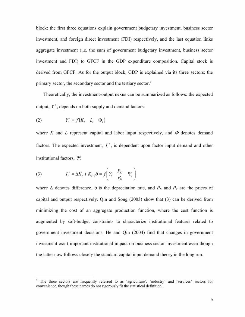
Theoretically, the investment-output nexus can be summarized as follows: the expected
output, etY , depends on both supply and demand factors:
(2) ( )ttte
t LKfY Φ=
where K and L represent capital and labor input respectively, and Φ denotes demand
factors. The expected investment, etI , is dependent upon factor input demand and other
institutional factors, Ψ:
(3) ⎟⎟⎠
⎞⎜⎜⎝
⎛Ψ=+∆= − t
Yt
Ktttt
et P
PYfKKI δ1
where ∆ denotes difference, δ is the depreciation rate, and PK and PY are the prices of
capital and output respectively. Qin and Song (2003) show that (3) can be derived from
minimizing the cost of an aggregate production function, where the cost function is
augmented by soft-budget constraints to characterize institutional features related to
government investment decisions. He and Qin (2004) find that changes in government
investment exert important institutional impact on business sector investment even though
the latter now follows closely the standard capital input demand theory in the long run.
9 The three sectors are frequently referred to as ‘agriculture’, ‘industry’ and ‘services’ sectors for convenience, though these names do not rigorously fit the statistical definition.
10
Two issues are in need of clarification with equation (2). First, it does not contain an
explicit technological progress factor. This is due to two reasons. One is data evidence, i.e.
the lack of observable long-run trend shown in Figure 2.2 of the previous section. The other
is the lack of robust empirical evidence identifying total factor productivity, see e.g. (Chen
1997), (Easterly and Levine 2002) and (Carlaw and Lipsey 2003). One alternative is to
endogenize technological progress with respect to capital, as widely adopted in endogenous
growth theories. For example, King and Robson (1993) assume that it is a nonlinear
function of It. Since the dynamics of It is adequately incorporated in the econometric
specification of the equations corresponding to (3), our model has not ruled out the
possibility of investment-led technological changes.10 The second issue is concerned with
the feasibility of a production function dominant output equation to explain the output of
the three sectors individually. Apart from data unavailability with respect to disaggregate
capital inputs, it is questionable whether output of services is dominantly supply driven. In
the China model, only the secondary sector follows a long-run production function. The
other two sectors are explained mainly from the demand side, considering that labor input
does not serve as a constraint to either sector. A more detailed sketch of the output block,
as well as the investment block of the China model is given in Figure 3.1.
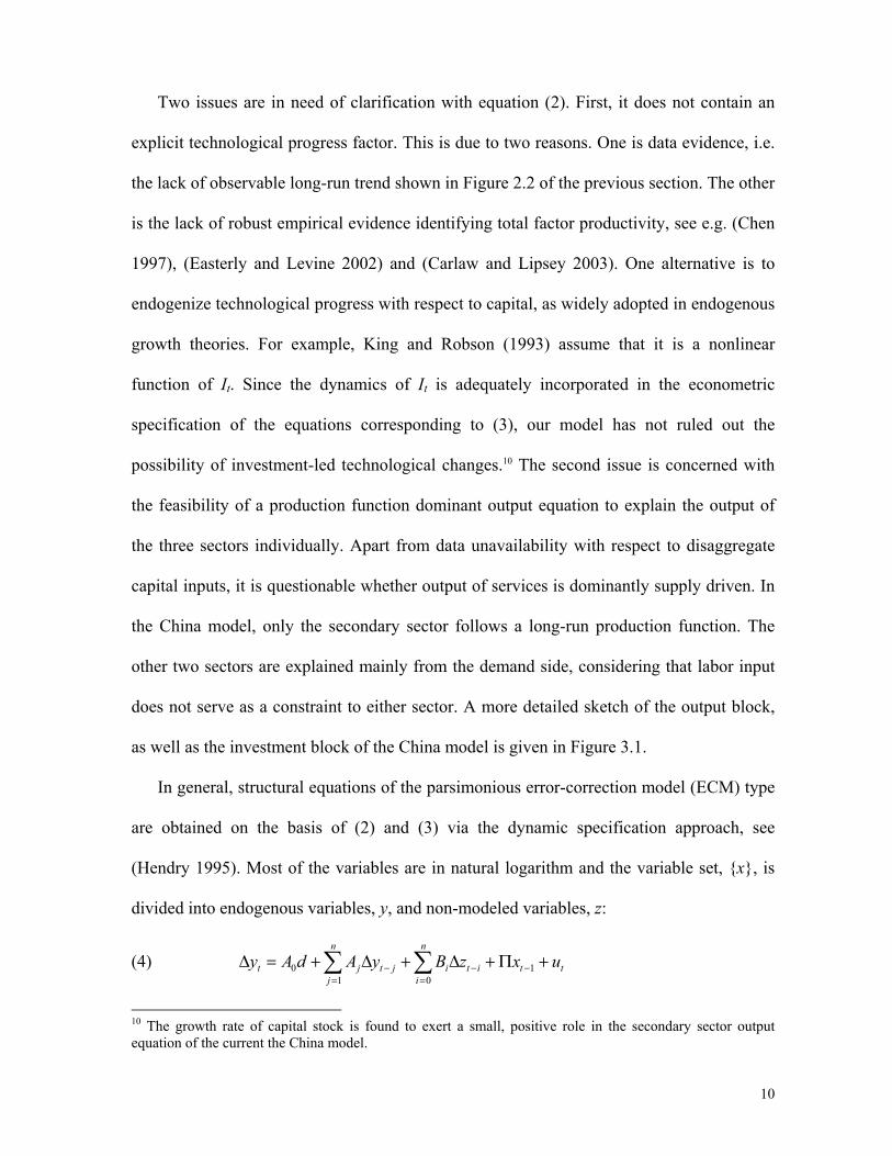
In general, structural equations of the parsimonious error-correction model (ECM) type
are obtained on the basis of (2) and (3) via the dynamic specification approach, see
(Hendry 1995). Most of the variables are in natural logarithm and the variable set, {x}, is
divided into endogenous variables, y, and non-modeled variables, z:
(4) ttit
n
iijt
n
jjt uxzByAdAy +Π+∆+∆+=∆ −−
=−
=∑∑ 1
010
10 The growth rate of capital stock is found to exert a small, positive role in the secondary sector output equation of the current the China model.
11
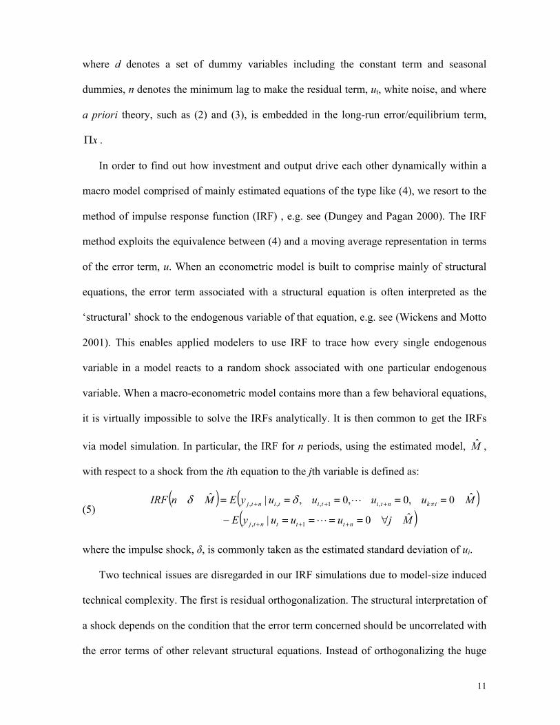
where d denotes a set of dummy variables including the constant term and seasonal
dummies, n denotes the minimum lag to make the residual term, ut, white noise, and where
a priori theory, such as (2) and (3), is embedded in the long-run error/equilibrium term,
xΠ .
In order to find out how investment and output drive each other dynamically within a
macro model comprised of mainly estimated equations of the type like (4), we resort to the
method of impulse response function (IRF) , e.g. see (Dungey and Pagan 2000). The IRF
method exploits the equivalence between (4) and a moving average representation in terms
of the error term, u. When an econometric model is built to comprise mainly of structural
equations, the error term associated with a structural equation is often interpreted as the
‘structural’ shock to the endogenous variable of that equation, e.g. see (Wickens and Motto
2001). This enables applied modelers to use IRF to trace how every single endogenous
variable in a model reacts to a random shock associated with one particular endogenous
variable. When a macro-econometric model contains more than a few behavioral equations,
it is virtually impossible to solve the IRFs analytically. It is then common to get the IRFs
via model simulation. In particular, the IRF for n periods, using the estimated model, M̂ ,
with respect to a shock from the ith equation to the jth variable is defined as:
(5) ( ) ( )
( )MjuuuyE
MuuuuyEMnIRF
ntttntj
ikntititintj
ˆ0|
ˆ0,0,0,|ˆ
1,
,1,,,
∀====−
=====
+++
≠+++
L
Lδδ
where the impulse shock, δ, is commonly taken as the estimated standard deviation of ui.
Two technical issues are disregarded in our IRF simulations due to model-size induced
technical complexity. The first is residual orthogonalization. The structural interpretation of
a shock depends on the condition that the error term concerned should be uncorrelated with
the error terms of other relevant structural equations. Instead of orthogonalizing the huge

12
residual matrix of the model, we simply check the sample covariance of those residuals
relevant to our IRF simulations. In most cases, the covariance is negligibly small. The
second issue is estimating confidence intervals for the IRFs. Although various methods are
available, it is practically infeasible for us to implement them on a model of this size.
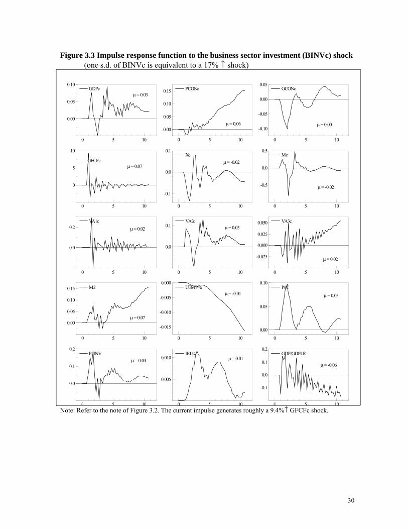
Three sets of IRFs are simulated to examine how much investment shocks impact on
the output. The first corresponds to a government budgetary investment shock, the second
to the business sector investment shock and the third to the combined shocks of the first
two. The results of IRFs relating to the major variables are illustrated in Figures 3.2, 3.3
and 3.4 respectively. In these figures, all the level variables are divided by population,
which is exogenous in the model to facilitate the interpretation of the simulation results
with respect to growth theories.
Several interesting observations can be made out of these IRF graphs. First, there is a
visible, though very small, lasting output gain from one-off investment shocks. Roughly, a
10% one-off increase in GFCF generates around 0.05% long-term GDP growth (see the
average as well as the end-of-sample value of GDPc in Figure 3.4). Second, the growth is
predominantly from the secondary sector (i.e. GDP growth path closely follows secondary
sector growth path), followed by a rising tertiary sector output. The primary sector enjoys
the least growth from the investment shocks. Third, the increase in the output of the tertiary
sector is accompanied by a decline in unemployment and a subsequent rise in private
consumption, implying certain long-term welfare gain of the shocks. This also shows that
the long-term growth effect can be sustained by enhanced, though delayed, demand factors,
even in the absence of technological progress (i.e. the graphs in the bottom right panels of
13
these figures show no discernible upward movement to indicate technological progress)11.
Fourth, government investment plays a pivotal role in the increase in output even though its
one-off increase is roughly equivalent to 0.4% GFCF shock, its long-term output impact is
as large as a 9.4% GFCF shock from the business sector investment. This is because an
increase in government investment signals expansionary fiscal policy to the economy,
invoking stronger growth in GFCF in the subsequent years (see Figure 3.2). Finally, there
are visible lags of reaction as well as substantial dampening of the initial investment shocks
(if the scales of volatility between the IRFs of GDP and GFCF are compared), which
further explains why investment volatilities are not visible in the output volatilities,
especially the simultaneous volatilities.
Since the increase in private consumption appears to play a crucial role in sustaining
the long-term GDP growth in the above scenarios, we experiment on a scenario where the
initial shock comes from private consumption in order to see if such a shock has similar
growth effect, see Figure 3.5. It is discernible from the IRFs in Figure 3.5 that the answer is
negative. A one-off increase in private consumption exerts no permanent effect on GDP
growth. This is not very surprising though as a one-off consumption increase does not have
the cumulative effect that a one-off investment increase has via capital stock.
Next, we simulate four sets of IRFs to output shocks. The first three sets correspond to
an impulse shock of the primary sector, the secondary sector and the tertiary sectors
respectively. The last set corresponds to combined shocks of these three sectors. The IRFs
of GFCF as well as the government investment and business investment are plotted in
Figure 3.6. In order to make the effects comparable across sectors, we normalized the
effects of sectoral shocks in Figure 3.6 by converting each sector shock into an equivalent 11 GDP/GDPLR in the bottom right panel is the de-trended GDP defined in Figure 2.2 and discussed in section II.
14
1% GDP growth shock.12 Notice that the output shocks virtually have no permanent effect
on investment. More interestingly, the volatilities that the output shocks induce on
investment variables are far smaller than those induced by investment shocks on output
variables. In particular, the primary sector is the sector that invokes the largest output-led
temporary investment spikes among the three sectors, whereas the temporary output rise in
the secondary and the tertiary sectors even results in negative investment demand in the
long run. In other words, only the agricultural sector appears relatively in need of further
investment. This is mainly due to the fact that nominal responses to each shock differ
across sectors because of different implicit impact on the three sectoral deflators, which
transmits onto various prices and interest rates. Figure 3.7 illustrates these differences
embodied in inflation (both in terms of consumer price and investment price indices),
nominal and real lending rates. It is discernible from the figure that agriculture is the only
sector whose shock dampens the real lending rate to stimulate investment. Taken as a
whole, the simulation results suggest that output-led investment is far more efficient than
autonomous investment rises if judged on the basis of relative incremental changes of
investment versus output growth. In other words, if investment depends purely on factor
input demand as shown in equation (2), less investment would be needed to sustain the
growth. The existing capacity in the economy appears to have room for further growth
without investment growth, e.g. see similar views by Wolf (2005).
The IRF results clearly show why the recent investment boom in China has not been
transmitted into the country’s GDP growth and why GDP growth has been more or less
12 After the normalization, the primary sector impulse shock generates roughly a 5% temporary rise and 0.25% permanent rise in GFCF; the secondary sector shock generates roughly a 2% temporary rise and 0.1% permanent fall in GFCF; the tertiary sector shock generates 2% temporary rise and 0.04% permanent fall in GFCF.
15
immune to investment fevers. It also substantiates the data evidences presented in the
previous section.
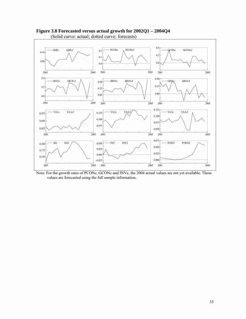
Would the recent investment boom have occurred if the economy did not encounter any
autonomous policy changes or internal shocks? To examine this we run a model forecast
for the period 2002Q1 to 2004Q4 and assumed zero shocks for all equations, with the
domestic and exogenous variables following their 2001 dynamics, and allowed the world
exogenous variables to take their observed values. The forecasted values of key variables
are plotted in Figure 3.8, together with the actual values. As seen from this figure, the
economy would have run slightly smoother, the GDP would have grown at 8.4% on
average instead of 9%, and the growth in GFCF would have been 18% instead of above
21% on average for the three years. It appears that GDP growth is certainly hardly affected
by a much reduced investment speed (about 15% drop).
IV. Conclusions
This paper assesses empirically the validity of the belief that the Chinese economy still
follows largely the investment-led growth paradigm. The paradigm is scrutinized from
several aspects of the investment-output nexus: the lead-lag relationship between the
growth rates of the pair, the simultaneity and long-run interdependency between the pair in
levels, and the combined long-run and short-run interactions between them when both are
endogenized within a macroeconometric model. The effects of investment are considered
not only as GFCF flows but also as cumulated capital stock. Furthermore, the nexus is
examined at a disaggregate level by means of impulse response function analysis of a
macroeconometric model. Specifically, the dynamics of the nexus is examined through the
impacts of random shocks via government budgetary investment, business sector
investment, as well as three output sectors.

16
The data analyses and model simulations yield a number of interesting results with
important policy implications:
1. Empirical results show the existence of a long-run positive relationship between
investment and economic growth, but the causality runs from the latter to the
former. In other words, the growth of capital stock and/or growth of investment
does not lead or exogenously drive output growth regularly either in short run or in
long run. Rather, it is output that drives investment demand in the economy. This
implies the applicability of market-based growth theories.
2. Analysis of the long-run GDP trend shows that the Chinese economy has not been
an exception to the East Asian ‘miracle’, in the sense that there lacks evidence of
noticeably long-lasting technological progress to refute the constant return to scale
condition in the long run. Indeed, rapid investment growth has resulted in rising
capital-output ratio rather than output growth acceleration — another reason why
investment is not really driving growth.
3. Rising capital-output ratio indicates the problem of overinvestment, a problem
impinging on the issue of investment efficiency at a macro level. The severity of the
problem is further highlighted by the model simulation results. Specifically, the
investment growth to output growth ratio is significantly higher when the random
shock originates from investment than when the shock originates from output; a
random increase of investment leads to further rise in capital-output ratio over a
long period. Overinvestment in the sense of increasing investment irrespective of
output expectations would give rise to more efficiency loss and structural imbalance
in the economy than to more economic growth, especially when there is surplus

17
capital capacity. This helps explain why investment-led overheating would heat
inflation far more easily than output.
4. The model simulation results at the sectoral level shed further light to the above
point. Among the three sectors, agriculture is the sector whose growth would
demand the highest investment incremental. In contrast, the secondary sector can
sustain further growth even with a slight reduction in investment, implying that
surplus capital capacity is more prevalent in this sector.
5. Disaggregate model simulation on the investment side also shows that the
government budgetary investment plays a key role in generating investment fever,
i.e. overinvestment irrespective of output expectations. As government investment
serves as an important signal of fiscal policy, a small increase could trigger sizeable
domestic investment expansion, resulting in a much amplified investment
oscillation. The ensuing long-run overcapacity in terms of GDP gap can be more
severe than that induced by an increase originated from the business-sector
investment. On the other hand, the positive effect of government investment on
GDP growth endorses the recent theoretical studies on fiscal policy and economic
growth, e.g. see (Zagler and Dürnecker 2003). It raises an importance issue of how
policy makers should balance the goals of reducing unemployment and enhancing
aggregate efficiency in investment and capital utilization. In principle, policy
makers need to give far more attention to the efficiency/productivity of investment
than to the magnitude of investment; they should provide the enabling environment
that would allow the economy to take advantage of expanded opportunities. This
entails sound measures to encourage technological progress and human capital
improvement, to enhance existing capacity utilization and to balance development
18
strategies among sectors, as well as to speed up capital market and banking sector
reforms.
6. Nevertheless, the view that investment drives output growth is verified in one
aspect, namely that a one-off increase in aggregate investment could generate
relatively long-lasting impact on the growth of output, albeit very small. More
interestingly, the growth is sustained by a much lagged rising consumption
response. This result reveals the long-term welfare gain that investment shocks
could generate, a practically more important issue, but somewhat less investigated,
than the existence of long-run balance growth, see (Temple 2003). It also shows
how the consumption side of an economy can play an important role, an area not
yet adequately explored in growth theories, see (George et al 2003). Moreover, it
offers a plausible way of demystifying the East Asian ‘miracle’. Therefore, it
appears right to say ‘yes’ to the investment-led growth view under this
circumstance, although such a growth strategy may not be optimal for the Chinese
economy.
Acknowledgements
This paper is an extension of a short piece, originally written by Qin and Quising as a
Policy Brief at ADB. Thanks are due to I. Ali, D. Brooks, X.-Q. Fan, C.-Y, Park, J.-P.
Verbiest, and Y.-D. Yu for their valuable comments on that short piece. We are also
grateful to G. Ducanes, S.-G. Liu, and N. Magtibay-Ramos for their substantial help in
developing the ADB China model. Thanks should also be extended to participants of
EcoMod2005 Conference, where the paper was presented and received helpful
comments.

19
Appendix: Data Description and Sources
Variables Description Source*
BINV Business Sector Investment The total investment in fixed assets (TIFA) net of the
government investment (see below) CMEI
FDI Foreign Direct Investment FDI (Actually utilized), CMEI
GCF Gross Capital Formation Identity: GCFC + IS
GCON Government Consumption Computed from nominal annual data in CSY with
seasonal interpolations provided by NSBC GDP Gross Domestic Product CMEI GDPLR Long-run GDP Computed by Identity in the China Model
GFCF Gross Fixed Capital Formation Interpolated from nominal annual data in CSY using
the seasonal patterns of TIFA
GINV Government investment Sum of expenditure for capital construction and innovation funds of enterprises from the table of the government budgetary expenditures, CMEI
IRL% Lending Rate PBC
IS Computed from nominal annual data in CSY with
seasonal interpolations provided by NSBC
K Capital Computed by equation (3); the depreciation rate is
taken as 5% quarterly in the China Model M2 Broad Money PBC
M Imports Converted from nominal data in $ into RMB by spot
exchange rate, CMEI P#C Consumer Price Index Deflator for GCON and PCON, CMEI P#GDP GDP deflator CMEI P#INV Investment Price Index Deflator for investment series, CMEI
PCON Private Consumption Computed from nominal annual data in CSY with
seasonal interpolations provided by NSBC TIFA The total investment in fixed assets, CMEI
UEMP% Unemployment Rate Computed from labor force and employment; these
two series are computed from CSY
VA1 Value Added from the Primary
Sector CMEI
VA2 Value Added from the Secondary
Sector CMEI
VA3 Value Added from the Tertiary
Sector CMEI
X Exports Converted from nominal data in $ into RMB by spot
exchange rate, CMEI
All data series are quarterly. To denote variables of constant price, a lower case ‘c’ is added at the end of the variable names. * CMEI stands for China Monthly Economic Indicators. CSY stands for China Statistical Yearbook. NSBC
stands for National Statistical Bureau of China. PBC stands for People’s Bank of China.

20
References Agénor, P. R. (2000) The Economics of Adjustment and Growth, San Diego: Academic
Press.
Ball, M., Morrison, T. and Wood, A. (1996) Structures investment and economic growth:
A long-term international comparison, Urban Studies, 33, 1687-706.
Blomström, M., Lipsey, R. E. and Zejan, M. (1996) Is fixed investment the key to
economic growth? Quarterly Journal of Economics, 111, 269-76.
Carlaw, K. I. and Lipsey, R. G. (2003) Productivity, technology and economic growth:
What is the relationship? Journal of Economic Surveys, 17, 457-95.
Chen, E. K. Y. (1997) The total factor productivity debate: Determinants of economic
growth in East Asia, Asian-Pacific Economic Literature, 11, 18-38.
Dungey, M. and Pagan, A. (2000) A structural VAR model of the Australian economy, The
Economic Record, 76, 321-42.
Easterly, W. and Levine, R. (2002) It’s not factor accumulation: Stylized facts and growth
models, Central Bank of Chile Working Papers, no. 164.
George, D. A. R., Oxley, L. and Carlaw, K. (2003) Economic growth in transition, Journal
of Economic Surveys, 17, 227-37.
Goldstein, M. and Lardy, N. R. (2004) What kind of landing for the Chinese economy?
Institute for International Economics Policy Briefs, 04-7.
He, X.-H. and Qin, D. (2004) Aggregate investment in People’s Republic of China: Some
empirical evidence, Asian Development Review, 21, 99-117.
He, X.-H., Qin, D. and Quising, P. (2004) Macroeconometric model of China: Summary
Report, mimeo, ERMF, Asian Development Bank.
Hendry, D. F. (1995) Dynamic economics, Oxford: Oxford University Press.
Imai, H. (1994) China’s endogenous investment cycle, Journal of Comparative Economics,
19, 188-216.
King, M. A. and Robson, M. H. (1993) A dynamic model of investment and endogenous
growth, Scandinavian Journal of Economics, 95, 445-66.
Kornai, J. (1980) The Economics of Shortage, Amsterdam: North-Holland.
Li, C.-W. (2000) Endogenous vs. Semi-Endogenous Growth in a Two-R&D-Sector Model,
Economic Journal, 110, 109-22.
21
Lin, J. Y. (2004) Is China’s growth real and sustainable? Working Paper Series E2004003,
China Center for Economic Research, Peking University.
Kwan, A. C. C., Wu, Y.-R. and Zhang, J.-X. (1999) Fixed investment and economic
growth in China, Economics of Planning, 32, 67-79.
Qin, D. and Song, H.-Y. (2003) Excess Investment and Efficiency Loss during Reforms:
The Case of Provincial-level Fixed-asset Investment in China, ADB ERD Working
Paper Series, no 47; also (in Chinese) China Economics Quarterly, 2, 807-32.
Qin, D., He, X-H, Liu, S-G and Quising, P. (2005) Modelling Monetary Transmission and
Policy in People’s Republic of China, Journal of Policy Modeling, 27, 157-75.
Rebelo, S. T. (1991) Long run policy analysis and long run economic growth, Journal of
Political Economy, 99, 500-21.
Senhadji, A. (2000) Sources of economic growth: An extensive growth accounting
exercises, IMF Staff Papers, 47, 129-57.
Temple, J. (1999) The new growth evidence, Journal of Economic Literature, 37, 112-56.
Temple, J. (2003) The long-run implications of growth theories, Journal of Economic
Surveys, 17, 497-514.
Wichens, M. R. and Motto, R. (2001) Estimating shocks and impulse response functions,
Journal of Applied Econometrics, 16, 371-87.
Wolf, M. (2005) China has further to grow to catch up with the world, Financial Times,
April 13, p13.
Young, A. (1995) The tyranny of numbers: Confronting the statistical realities of the East
Asian growth experience, Quarterly Journal of Economics, 110, 641-80.
Yu, Q. (1998) Capital investment, international trade and economic growth in China:
Evidence in the 1980-90s, China Economic Review, 9, 73-84.
Zagler, M. and Dürnecker, G. (2003) Fiscal policy and economic growth, Journal of
Economic Surveys, 17, 397-418.
Zhang, J. (2003) Investment, investment efficiency, and economic growth in China, Journal
of Asian Economics, 14, 713-34.
22
Table 1.1 China's Investment Ratios, 1978-2004
Year GFCF % to GDP
GCF % to GDP Year GFCF% to
GDP GCF % to
GDP
1978 29.8 38.2 1992 32.2 37.3 1979 28.3 36.2 1993 37.6 43.5 1980 29.0 34.9 1994 36.1 41.3 1981 25.6 32.3 1995 34.7 40.8 1982 27.2 32.1 1996 34.2 39.3 1983 28.1 33.0 1997 33.6 38.0 1984 29.7 34.5 1998 35.0 37.4 1985 30.0 38.5 1999 35.7 37.1 1986 30.6 38.0 2000 36.5 36.4 1987 31.8 36.7 2001 37.3 38.0 1988 31.4 37.4 2002 38.9 39.2 1989 26.4 37.0 2003 42.2 42.3 1990 25.8 35.2 2004 /a 44.0 44.1 1991 27.9 35.3
AVERAGE 32.6 37.5 a/ ADB Staff Estimate Note: GCF denotes GFCF plus inventory or change in stocks; Source: China Statistical Yearbook, 2004; "Stable and Rapid Development of the National Economy in 2004" available at http://www/stats.gov.cn; ADB Database
Table 1.2 Average Investment Ratios for Selected Economies
GFCF % to GDP GCF % to GDP
Sample: 1978—2004 Hong Kong, China 27.2 28.4 Korea, Rep of 30.7 31.1 Singapore 35.5 36.0 Taiwan 20.0 20.6 USA 15.9 19.8 Sample: 1980—2004 Japan 27.7 28.0 Source: CEIC Data Company Ltd.

23
Table 2.1 Granger-Causality tests on GFCF & GDP and Capital & GDP Endogenous Variable F-statistic Lag coefficients Investment and GDP growth rates (in real terms) GDPc(-1) GDPc(-2) GDPc(-3) GDPc(-4)
GFCFc 0.9892 1.5596 -0.585 -2.2139 0.7603 [0.4280] (1.3950) (1.4860) (1.5600) (1.4280)
GFCFc(-1) GFCFc(-2) GFCFc(-3) GFCFc(-4) GDPc 1.3944 0.0235 0.0185 -0.0056 0.0283
[0.2589] (0.0250) (0.0194) (0.0188) (0.0186)
Capital and GDP growth rates (in real terms) GDPc(-1) GDPc(-2) GDPc(-3) GDPc(-4)
Kc 2.6077 0.0392 -0.0337 0.0052 0.1929 [0.0547] (0.1004) (0.1068) (0.1107) (0.0934)*
Kc(-1) Kc(-2) Kc(-3) Kc(-4) GDPc 1.3117 0.0752 -0.0233 -0.0513 -0.0733
[0.2874] (0.2175) (0.3519) (0.3302) (0.1773) Note: indicates growth rate. Statistics in parentheses are standard errors while those in brackets
are probabilities. Those marked by ‘*’ are significant at 5% level. F-statistic indicates no granger-causality between GFCF growth and GDP growth or capital growth and GDP growth. GDP growth marginally granger-causes capital growth (the significant level is 5.5%).
Table 2.2 Dickey-Fuller (DF) and Augmented Dickey-Fuller (ADF) unit-root tests Full sample Sub-sample
DF [-2.92 at 5%]
ADF(3) [-2.93 at 5%]
DF [-2.94 at 5%]
ADF(3) [-2.94 at 5%]
( )GDPcln4∆ -2.508 -2.919 -4.112 -3.601 ( )GFCFcln4∆ -5.004 -3.462 -4.843 -1.95 ( )Kcln4∆ -2.823 -6.368 -0.8857 -1.245
( )GDPcln -1.423 -4.619 -0.6333 -1.071 ( )GFCFcln -1.793 -1.531 -1.366 -2.616 ( )Kcln 1.889 -0.2317 -2.147 -4.791
Note: Full sample for GDPc: 1992 – 2004, for GFCFc and Kc: 1992 – 2003; Sub-sample cuts off the first three years: 1992 – 1994. Seasonal dummies are included for all the level variable tests. Critical values are in squared brackets.

24
Table 2.3 Cointegration Analysis Model includes: Constant & Seasonals Constant, Trend & Seasonals Set 1. GFCF and GDP rank = 0 Trace test 33.16** 48.77** Maximum Eigenvalue test 29.54** 36.44** rank = 1 Trace test 3.63 12.34 Maximum Eigenvalue test 3.63 12.34 Unit Root test on residuals Durbin-Watson 2.44 2.26 t-ADF -8.866** -6.528** Set 2. Capital and GDP rank = 0 Trace test 56.37 64.20** Maximum Eigenvalue test 55.67 60.85** rank = 1 Trace test 0.7 3.35 Maximum Eigenvalue test 0.7 3.35 Unit Root test on residuals Durbin-Watson 2.41 1.92 t-ADF 7.120** -4.763** Note: There is at least one cointegrating equation for GFCF and GDP and capital and GDP. Due to
small sample size, some residuals were found to be non-stationary depending on the numberof lags included in the ADF test. For the purposes of this study, only the results which include lags that render the t-ADF statistics significant are reported.
25
Table 2.4 Simultaneous equations VAR model versus Single equations OLS Model
Endogenous Variable Coefficients
Set 1. GFCF and GDP Simultaneous equations VAR model
GDPc(-1) GFCFc GFCFc(-1) Constant Seasonal(1) Seasonal(3) GDPc 1.0504 -0.0481 -0.0034 -0.1943 -0.7288 -0.1503 (0.0423)* (0.0506) (0.0282) (0.2314) (0.1037)* (0.0283)*
GFCFc(-1) GDPc GDPc(-1) Constant Seasonal(1) Seasonal(3) GFCFc 0.0611 4.6497 -3.3158 -6.9182 1.1044 -0.4237 (0.1992) (0.4800)* (0.5658)* (1.6240)* (0.2937)* (0.1335)*
OLS model GDPc(-1) GFCFc GFCFc(-1) Constant Seasonal(1) Seasonal(3) GDPc 1.0243 -0.0108 -0.0219 0.2950 -0.6528 -0.1302 (0.0274)* (0.0230) (0.0168) (0.1909) (0.0480)* (0.0144)*
INVc(-1) GDPc GDPc(-1) Constant Seasonal(1) Seasonal(2) GFCFc 0.0506 4.0685 -2.7202 -6.9001 0.7702 -0.3797 (0.1948) (0.4390)* (0.5265)* (1.5880)* (0.2708)* (0.1300)*
Set 2. Capital and GDP Simultaneous equations VAR model
GDPc(-1) Kc Kc(-1) Constant Seasonal(1) Seasonal(3) GDPc 1.0842 -0.9150 0.8657 -0.1193 -0.7318 -0.1611 (0.0985)* (0.4679) (0.4177)* (0.5251) (0.0547)* (0.0189)*
Kc(-1) GDPc GDPc(-1) Constant Seasonal(1) Seasonal(2) Kc 0.7924 0.1868 0.2007 -2.1100 -0.0191 0.0532 (0.0206)* (0.0365)* (0.0609)* (0.1931)* (0.0249) (0.0114)*
OLS model
GDPc(-1) Kc Kc(-1) Constant Seasonal(1) Seasonal(3) GDPc 0.9762 -0.3871 0.3947 0.4507 -0.6710 -0.1410 (0.0534)* (0.2377) (0.2125) (0.2899) (0.0287)* (0.0109)*
Kc(-1) GDPc GDPc(-1) Constant Seasonal(2) Seasonal(3) Kc 0.7863 0.1594 0.2389 -2.1594 -0.0370 0.0582 (0.0202)* (0.0341)* (0.0580)* (0.1903)* (0.0234) (0.0111)*
Note: Statistics in parentheses are standard errors. Those marked by ‘*’ are significant at the 5% level. GFCF is not significant to GDP in set 1. Capital is significant to GDP in set 2 with different coefficients for the simultaneous and OLS models implying interdependence with GDP. GDP is however found to be weakly exogenous to investment (set 1) and capital (set 2).
26
Figure 1.1 Average Growth of Real GFCF for Selected Economies
1995-2004
0
2
4
6
8
10
12
Hong Kon
g, C
hina
Japa
n
Korea
Singa
pore
Taipei,C
hina
PRC
%
Source: CEIC Data Company Ltd.; China Statistical Yearbook, 2004
Figure 1.2 Growth rates of GDP, GFCF and TIFA (all in constant prices)
-10.0%
0.0%
10.0%
20.0%
30.0%
40.0%
1990 1991 1992 1993 1994 1995 1996 1997 1998 1999 2000 2001 2002 2003 2004
GDPc GFCFc TIFAc
Data source: See the Appendix.
27
Figure 2.1 Co-movement of Growth of GDP and its components
-6.0
-4.0
-2.0
0.0
2.0
4.0
6.0
8.0
10.0
12.0
14.0
16.0
1993 1994 1995 1996 1997 1998 1999 2000 2001 2002 2003
Y C GFCF NX IS
Note: Weighted growth rates of the components are presented here alongside GDP growth. Source: CMEI for GDP and components in levels
Figure 2.2 GDPc – Actual, Long-run and Actual net of long-run
0
500000
1000000
1500000
2000000
2500000
3000000
3500000
199201 199401 199601 199801 200001 2002010.0
0.5
1.0
1.5
2.0
2.5
GDP
GDPLR
GDP net of LR
Note: GDP net of LR refers to detrended GDP which is taken as the ratio between GDP and GDPLR.
28
Figure 3.1 Framework of output and investment blocks of the China Model
where:
BINVc = f ( GDP, Government investment )
FDI = f ( Differential interest rates, Trade openness, Relative prices )
User cost of capital,
GINVc = f ( Revenue, )(unemployment rate,
GDP gap)
Policy targets
GFCFc FDIcGINVc(Government investment)
BINVc(Business
investment)
= f ( )++(Foreign direct
investment)
(additional short-run factor)
GDPc(Serv ices)
VA3cVA2c +(Industry)
+VA1c(Agriculture)
=
where:
VA1c = f ( Income, Relative Prices, Sector Structural Shifts )(demand side function) (additional short-run factor)
VA2c = f ( Capital, Labor, Sector Structural Shifts )(supply side function) (additional short-run factor)
VA3c = f ( Income, Relative Prices, Sector Structural Shifts )(supply side function) (additional short-run factor)

29
Figure 3.2 Impulse response function to government investment (GINVc) shock
(one standard deviation (s.d.) of GINVc is equivalent to a 10% ↑ shock)
0 5 10
0.000
0.025
0.050
0.075
µ = 0.03GDPc
0 5 10
0.0
0.1
0.2
µ = 0.07
PCONc
0 5 10
-0.05
0.00
0.05
µ = -0.01
GCONc
0 5 10
0
1
2
µ = 0.09---- GFCFc
0 5 10
-0.10
-0.05
0.00
0.05
µ = -0.02
Xc
0 5 10
-0.2
0.0
0.2 µ = -0.02Mc
0 5 10
0.00
0.05
0.10 µ = 0.02VA1c
0 5 10
0.00
0.05
0.10 µ = 0.04VA2c
0 5 10
0.000
0.025
0.050
0.075
µ = 0.02
VA3c
0 5 10
0.1
0.2
µ = 0.07M2
0 5 10
-0.015
-0.010
-0.005
0.000
µ = -0.01UEMP%
0 5 10
0.05
0.10
µ = 0.03P#C
0 5 10
0.05
0.10
0.15µ = 0.05
P#INV
0 5 10
0.005
0.010
0.015µ = 0.01
IRL%
0 5 10
-0.2
-0.1
0.0
0.1
µ = -0.05GDP/GDPLR
Note: The experiment is carried out for an 11-year (44 quarters) period. The impulse is imposed at quarter 5 and there are 40 quarters of response time. The unit of the vertical axis is in percentage. All the level variables are divided by population. The curves capture the difference of annual growth rates of the variables concerned and the µ ’s are estimated average values. See the appendix for detailed definitions of the variables. The current impulse generates roughly a 0.4%↑ GFCFc shock.
30
Figure 3.3 Impulse response function to the business sector investment (BINVc) shock
(one s.d. of BINVc is equivalent to a 17% ↑ shock)
0 5 10
0.00
0.05
0.10
µ = 0.03GDPc
0 5 10
0.00
0.05
0.10
0.15
µ = 0.06
PCONc
0 5 10
-0.10
-0.05
0.00
0.05
µ = 0.00
GCONc
0 5 10
0
5
10
µ = 0.07----- GFCFc
0 5 10
-0.1
0.0
0.1
µ = -0.02Xc
0 5 10
-0.5
0.0
0.5
µ = -0.02
Mc
0 5 10
0.0
0.2 µ = 0.02VA1c
0 5 10
0.0
0.1 µ = 0.03VA2c
0 5 10
-0.025
0.000
0.025
0.050
µ = 0.02
VA3c
0 5 10
0.00
0.05
0.10
0.15
µ = 0.07
M2
0 5 10
-0.015
-0.010
-0.005
0.000
µ = -0.01UEMP%
0 5 10
0.00
0.05
0.10
µ = 0.03
P#C
0 5 10
0.0
0.1
0.2
µ = 0.04P#INV
0 5 10
0.005
0.010 µ = 0.01IRL%
0 5 10
-0.1
0.0
0.1
0.2
µ = -0.06
GDP/GDPLR
Note: Refer to the note of Figure 3.2. The current impulse generates roughly a 9.4%↑ GFCFc shock.

31
Figure 3.4 Impulse response function to the combined investment shocks
(10% ↑ shock in GINVc; 17% ↑ shock in BINVc)
0 5 10
0.00
0.05
0.10
µ = 0.06
GDPc
0 5 10
0.0
0.1
0.2
0.3
µ = 0.13
PCONc
0 5 10
-0.1
0.0
0.1
µ = -0.01
GCONc
0 5 10
0
5
10
µ = 0.16
------- GFCFc
0 5 10
-0.1
0.0
µ = -0.05Xc
0 5 10
-0.5
0.0
0.5 Mc
0 5 10
0.0
0.2
0.4
µ = 0.04VA1c
0 5 10
0.0
0.1
0.2µ = 0.07
VA2c
0 5 10
0.00
0.05
0.10
µ = 0.03
VA3c
0 5 10
0.0
0.1
0.2
0.3
0.4
µ = 0.14
M2
0 5 10
-0.03
-0.02
-0.01
0.00
µ = -0.01UEMP%
0 5 10
0.05
0.10
0.15
µ = 0.06P#C
0 5 10
0.0
0.1
0.2 µ = 0.09P#INV
0 5 10
0.01
0.02 µ = 0.01IRL%
0 5 10
-0.25
0.00µ = -0.11
GDP/GDPLR
Note: The same as the note of Figure 3.2. The current impulse generates roughly a 9.8%↑ GFCFc shock.

32
Figure 3.5 Impulse response function to the private consumption shocks
(4% ↑ shock in PCCONr; 3% ↑ shock in PCCONu)
0 5 10
0.00
0.02
0.04
µ = 0.00GDPc
0 5 10
-2.5
0.0
2.5µ = 0.00
PCONc
0 5 10
-0.01
0.00
0.01
µ = 0.00
GCONc
0 5 10
-0.1
0.0
0.1
µ = 0.00
------- GFCFc
0 5 10
-0.01
0.00
0.01
µ = 0.00
Xc
0 5 10
0.000
0.025
0.050
µ = 0.00Mc
0 5 10
0.0
0.1
0.2 µ = 0.00VA1c
0 5 10
-0.02
-0.01
0.00
0.01
µ = 0.00
VA2c
0 5 10
-0.0025
0.0000
0.0025
µ = 0.00VA3c
0 5 10
-0.2
0.0
µ = -0.02
M2
0 5 10
0.0000
0.0005
0.0010
µ = 0.00
UEMP%
0 5 10
-0.01
0.00
0.01
µ = 0.00
P#C
0 5 10
-0.01
0.00
0.01
µ = 0.00
P#INV
0 5 10
0.0000
0.0025
0.0050 µ = 0.00IRL%
0 5 10
0.000
0.025
0.050
µ = 0.01GDP/GDPLR
Note: The same as the note of Figure 3.2.

33
Figure 3.6 Impulse response function to GDPc impulse shock
1st row: 1 s.d. shock from VA1c generates roughly 0.044% ↑ GDP shock 2nd row: 1 s.d. shock from VA2c generates roughly 1.17% ↑ GDP shock 3rd row: 1 s.d. shock from VA3c generates roughly 0.45% ↑ GDP shock 4th row: combination of the three generates roughly 1.68% ↑ GDP shock
0 5 10
-1
0
1
µ = -0.07
µ = 0.16
µ = -0.15
GFCFc1
0 5 10
-2.5
0.0
µ = 0.14BINVc1
0 5 10
-0.5
0.0
0.5
1.0µ = -0.03
GINVc1
0 5 10
-1
0
1
2µ = -0.09
µ = 0.14
GFCFc2
0 5 10
-2.5
0.0
2.5 µ = -0.19BINVc2
0 5 10-0.5
0.0
0.5 µ = -0.05
µ = -0.02
GINVc2
0 5 10
-1
0
µ = -0.05GFCFc3
0 5 10
-2
0
µ = -0.08BINVc3
0 5 10-0.5
0.0
0.5 µ = 0.04GINVc3
0 5 10-1
0
1GFCFc123
0 5 10
-2.5
0.0
2.5 BINVc123
0 5 10-0.5
0.0
0.5GINVc123
Note: Refer to the note of Figure 3.2. The number added to the variable notation indicates the sector where shock is originated. To make the three sector shocks comparable, all the IRFs are rescaled to correspond to 1% of GDPc growth.

34
Figure 3.7 Nominal response to impulse shocks of the three sectors
(solid curve: by VA1c; dotted curve: by VA2c; dashed curve: by VA3c)
0 5 10
-0.1
0.0
0.1
0.2
0.3 Inflation_consumer
0 5 10-0.2
0.0
0.2
0.4Inflation_investment
0 5 10
-0.01
0.00
0.01
0.02Lending rate
0 5 10
-0.2
0.0
0.2 Real lending rate
Note: The unit of the vertical axis is in percentage. Inflation is calculated as y-o-y growth rates. See Figure
3.6 for the details of the impulse shock scenarios.
35
Figure 3.8 Forecasted versus actual growth for 2002Q1 – 2004Q4 (Solid curve: actual; dotted curve: forecasts)
2001 2005
0.08
0.10GDPc GDPcf
2001 2005
0.0
0.1
0.2 PCONc PCONcf
2001 2005
0.0
0.2
0.4GCONc GCONcf
2001 2005
0.0
0.2
0.4GFCFc GFCFcf
2001 2005
0.00
0.25
0.50 BINVc BINVcf
2001 2005
0.00
0.25
0.50GINVc GINVcf
2001 2005
0.025
0.050
0.075 VA1c VA1cf
2001 2005
0.075
0.100
0.125 VA2c VA2cf
2001 2005
0.050
0.075
0.100
0.125VA3c VA3cf
2001 2005
0.150
0.175
0.200 M2 M2f
2001 2005
-0.025
0.000
0.025
0.050 P#C P#Cf
2001 2005
0.000
0.025
0.050
0.075P#INV P#INVf
Note: For the growth rates of PCONc, GCONc and INVc, the 2004 actual values are not yet available. These values are forecasted using the full sample information.

This working paper has been produced bythe Department of Economics atQueen Mary, University of London
Copyright © 2005 Duo Qin, Marie Anne Cagas,
Department of Economics Queen Mary, University of LondonMile End RoadLondon E1 4NSTel: +44 (0)20 7882 5096Fax: +44 (0)20 8983 3580Web: www.econ.qmul.ac.uk/papers/wp.htm
Pilipinas Quising and Xin-Hua He. All rights reserved
Top Related