


Línguas
Páginas
Legal


Attitude Determination Using Multiple L1 GPS Receivers
João Miguel Mendes Cóias
Dissertação para obtenção do Grau de Mestre em Engenharia Aeroespacial
Júri
Presidente: Prof. Doutor João Manuel Lage de Miranda Lemos
Orientador: Prof. Doutor Paulo Jorge Coelho Ramalho Oliveira
Co-orientador: Prof. Doutor José Eduardo Charters Ribeiro da Cunha Sanguino
Vogal: Prof. Doutor Fernando Duarte Nunes
Maio 2012

i

ii
AGRADECIMENTOS
O concluir de uma tese de mestrado é o culminar de um processo, repleto de obstáculos, que nunca
seria possível de alcançar por conta própria. Assim, é inevitável endereçar os meus agradecimentos a
todos os que, com o seu importante contributo, tornaram possível chegar até aqui.
Ao Professor Paulo Oliveira e ao Professor José Sanguino, que sempre se mostraram disponíveis
para partilhar o seu conhecimento e cuja orientação foi essencial para seguir sempre o caminho certo
e ultrapassar os mais difíceis obstáculos.
À namorada, aos pais, à irmã e à restante família, que demonstraram sempre apoio incondicional e
ajudaram a ter uma visão mais optimista nos momentos mais difíceis.
Aos colegas de laboratório pelo companheirismo e entreajuda durante esta dura jornada.
A todos os restantes amigos que, perto ou longe, sempre demonstraram total apoio.
A todos, um sincero obrigado.
Esta tese de mestrado foi elaborada com o apoio parcial do Instituto de Telecomunicações (IT) e da
Fundação para a Ciência e Tecnologia (FCT), no âmbito do projecto PTDC/EEA-TEL/122086/2010.
iii
RESUMO
O uso de múltiplos receptores de GPS (Global Positioning System) permite a determinação de
posicionamento relativo, isto é, a determinação do vector posição entre a antena de referência e as
restantes. Para atingir níveis elevados de exatidão e precisão é necessário o uso de medições de
fase. Contudo, estas medições contêm uma ambiguidade inteira. A determinação da ambiguidade de
fase é um problema normalmente resolvido recorrendo a receptores de dupla frequência L1/L2.
Devido ao elevado custo destes receptores, existe uma necessidade de desenvolver técnicas para
resolver este problema usando receptores mais baratos de frequência única L1. Com o intuito de
determinar correctamente a ambiguidade de fase com receptores de frequência única, nesta
dissertação é proposto o uso do método de LAMBDA e o uso do Ambiguity Filter, permitindo a
determinação do vector de posicionamento relativo com precisões milimétricas. As melhorias do
Ambiguity Filter, propostas nesta dissertação, demonstraram um aumento da confiança na correcta
determinação da ambiguidade de fase e, consequentemente, na determinação do vector de
posicionamento relativo, e permitiram a adaptação às variações na constelação de satélites sem que
fosse perdida a solução milimétrica do vector de posicionamento relativo.
Através da combinação de diversos vectores de posicionamento relativo, com normas conhecidas,
obtidos utilizando quatro receptores L1, colocados em posições previamente conhecidas, é possível
determinar os ângulos de atitude de um corpo rígido com elevados níveis de exatidão e precisão.
Assim, são propostos dois modelos, um utilizando o método dos mínimos quadrados e a matriz de
rotação, e o segundo utilizando um Filtro de Kalman Estendido para estimar o quaternião de rotação.
As duas técnicas demonstraram bons resultados, permitindo a determinação dos ângulos de atitude
com precisões inferiores a 1°, em cenários susceptíveis à presença de multi-percurso.
Todos os resultados apresentados foram obtidos com recurso a dados reais.
Palavras-chave: ambiguidade de fase inteira, Ambiguity Filter, determinação de atitude, duplas
diferenças, GPS, método LAMBDA.

iv
ABSTRACT
The use of multiple Global Positioning System (GPS) receivers allows the determination of relative
position, that is, the baseline vector between a reference antenna and the remaining ones. To achieve
high levels of accuracy and precision it is mandatory the use of the carrier-phase measurements.
However, these measurements are biased by an unknown integer ambiguity. The integer ambiguity
determination problem is usually addressed in a context of dual-frequency L1/L2 receivers. Due to the
high cost of these receivers, strong motivations exist to explore techniques with cheaper single-
frequency L1 receivers. In order to correctly solve the integer ambiguity problem with L1 GPS
receivers, this thesis proposes the use of the LAMBDA method and the Ambiguity Filter, allowing the
determination of the baseline vector with millimeter level precision. Improvements proposed within the
Ambiguity Filter showed an increased confidence in the determination of the correct integer ambiguity,
and hence the baseline vector, and the adaptation to the dynamic variation of the satellites’
constellation, without the loss of the baseline solution with millimeter precision.
By combining multiple baselines, with known lengths, obtained by four L1 GPS receivers, placed in
known positions, it is possible to determine a rigid body’s attitude angles with high accuracy and
precision levels. Thus, two attitude determination techniques are presented, one using a Least
Squares estimation algorithm and the rotation matrix, and the second one using the rotation
quaternion that is determined resorting to an Extended Kalman Filter. Both techniques showed good
results allowing the determination of the attitude angles with precisions smaller than 1°, in scenarios
affected by multipath.
All the presented results were obtained with real data.
Keywords: Ambiguity Filter, attitude determination, double differences, GPS, integer ambiguity,
LAMBDA method.

v
ACRONYMS
ECEF Earth-Centered Earth-Fixed
EKF Extended Kalman Filter
ENU East North Up
GNSS Global Navigation Satellite Systems
GPS Global Positioning System
INS Inertial Navigation Systems
KF Kalman Filter
LoS Line of Sight
LS Least Squares
NED North East Down
RTK Real Time Kinematics
SBAS Satellite-Based Augmentation System
TD Triple Difference
UERE User Equivalent Range Error
WLS Weighted Least Squares
SYMBOLS
∆ Double Difference
Δ Single Difference
Pitch Angle
Mean
Standard Deviation
Heading Angle
Roll Angle

vi
INDEX AGRADECIMENTOS ............................................................................................................................................... ii
RESUMO ................................................................................................................................................................... iii
ABSTRACT .............................................................................................................................................................. iv
ACRONYMS .............................................................................................................................................................. v
SYMBOLS ................................................................................................................................................................. v
LIST OF FIGURES ................................................................................................................................................. viii
LIST OF TABLES ..................................................................................................................................................... xi
1 INTRODUCTION ............................................................................................................................................. 1
1.1 Motivation ................................................................................................................................................. 1
1.2 State of the Art .......................................................................................................................................... 1
1.3 Objectives and Structure ........................................................................................................................... 3
2 BASIC CONCEPTS .......................................................................................................................................... 5
2.1 Introduction ............................................................................................................................................... 5
2.2 Global Positioning System: Fundamentals and Operation ...................................................................... 5
2.3 Measurement Errors.................................................................................................................................. 7
2.3.1 Satellite Clock Error ............................................................................................................................. 7
2.3.2 Ephemeris Error ................................................................................................................................... 7
2.3.3 Relativistic Effects ............................................................................................................................... 7
2.3.4 Ionospheric Effects ............................................................................................................................... 8
2.3.5 Tropospheric Delay .............................................................................................................................. 8
2.3.6 Receiver Noise ..................................................................................................................................... 8
2.3.7 Multipath .............................................................................................................................................. 9
2.3.8 Pseudorange Error Budget ................................................................................................................... 9
2.4 Single Point Positioning ........................................................................................................................... 9
2.5 Coordinate Systems and Euler Angles ................................................................................................... 10
2.6 Accuracy and Precision .......................................................................................................................... 12
3 BASELINE DETERMINATION AND INTEGER AMBIGUITY RESOLUTION .................................... 13
3.1 Introduction ............................................................................................................................................. 13
3.2 System Definition ................................................................................................................................... 13
3.2.1 Observables ........................................................................................................................................ 13
3.2.2 Observation Model ............................................................................................................................. 15
3.2.3 Observables Covariance ..................................................................................................................... 17
3.3 Integer Ambiguity Resolution ................................................................................................................ 18
3.3.1 Float Solution ..................................................................................................................................... 19
3.3.2 Code Smoothing ................................................................................................................................. 19
3.3.3 LAMBDA Method ............................................................................................................................. 22
3.3.4 Ambiguity Filter ................................................................................................................................. 23
3.3.5 Constellation Changes: Recovery Techniques .................................................................................. 25
4 ATTITUDE DETERMINATION ................................................................................................................... 31
4.1 Introduction ............................................................................................................................................. 31

vii
4.2 Attitude Determination Using a Rotation Matrix .................................................................................. 31
4.3 Quaternion-Based Extended Kalman Filter for Attitude Determination ............................................... 33
4.3.1 Quaternion and Euler Angles ............................................................................................................. 33
4.3.2 Extended Kalman Filter ..................................................................................................................... 34
4.3.3 Reachability and Observability .......................................................................................................... 37
5 SOLUTION IMPLEMENTATION ................................................................................................................ 41
5.1 Introduction ............................................................................................................................................. 41
5.2 GPS Receivers and Antennas ................................................................................................................. 41
5.2.1 Magellan AC12 GPS Receivers ......................................................................................................... 41
5.2.2 U-Blox 6 GPS Receivers .................................................................................................................... 42
5.2.3 Antennas ............................................................................................................................................. 42
5.3 Algorithm Overview ............................................................................................................................... 43
5.4 Trials Description ................................................................................................................................... 45
5.4.1 Static Trials ......................................................................................................................................... 45
5.4.2 Dynamic Trial..................................................................................................................................... 47
6 RESULTS ........................................................................................................................................................ 49
6.1 Introduction ............................................................................................................................................. 49
6.2 Static Trials Results ................................................................................................................................ 49
6.2.1 Single Baseline Results ...................................................................................................................... 49
6.2.2 Multiple Baselines Results ................................................................................................................. 55
6.3 Dynamic Trial Results ............................................................................................................................ 66
7 CONCLUSIONS ............................................................................................................................................. 73
REFERENCES ......................................................................................................................................................... 75

viii
LIST OF FIGURES
Figure 1.1 – Illustration of the baselines’ definition .................................................................................................. 1
Figure 2.1 – Trilateration’s principle [18] ............................................................................................................... 10
Figure 2.2 – Body fixed frame ( ) ....................................................................................................................... 10
Figure 2.3 – ECEF frame and ENU frame, [24] ...................................................................................................... 11
Figure 2.4 – Euler angles: a) Body fixed frame rotation about the East axis (pitch angle); b) Body fixed frame
rotation about the North axis (roll angle); c) Body fixed frame rotation about the Down axis (heading angle). .. 12
Figure 2.5 – Illustration of both accuracy and precision concepts .......................................................................... 12
Figure 3.1 – Comparison between the triple differences of both carrier phase and code double differences ........ 15
Figure 3.2 – Zoom of the carrier-phase triple differences ....................................................................................... 15
Figure 3.3 – GPS interferometer for one satellite [1] .............................................................................................. 16
Figure 3.4 – Illustration of the KF loop ................................................................................................................... 20
Figure 3.5 – Carrier phase double differences evolution with a cycle slip, in static environment ......................... 26
Figure 3.6 – Carrier phase triple difference evolution with a cycle slip, in static environment ............................. 27
Figure 3.7 – Carrier phase double differences evolution without cycle slips, in static environment ..................... 27
Figure 3.8 – Carrier phase triple differences evolution without cycle slips, in static environment ....................... 28
Figure 3.9 – Histogram of triple differences without cycle slips, in static environment ........................................ 28
Figure 5.1 – a) AC12 sensor evaluation and development kit; b) AC12 OEM board [36] .................................... 41
Figure 5.2 – U-Blox 6 GPS receiver [37] ................................................................................................................ 42
Figure 5.3 – Novatel model 531 GPS antenna with Chocke Ring Model A032 [38] ............................................. 42
Figure 5.4 – NAIS magnetic antenna [36] ............................................................................................................... 43
Figure 5.5 – Flowchart of the developed algorithm................................................................................................. 44
Figure 5.6 – Top view of the antennas’ position, for the single baseline static trial (Google Earth, [40]) ............ 46
Figure 5.7 – GPS receivers’ disposition and baseline vectors ................................................................................. 46
Figure 5.8 – Top view of the platform’s orientation for the multiple baselines static trial (Google Earth, [40]) .. 47
Figure 5.9 – Top view of the platform’s path and orientation, for initial and final position, for the dynamic trial
(Google Earth, [40]) ................................................................................................................................................. 48
Figure 6.1 – Baseline length evolution, using the Ambiguity Filter’s metrics 1 and 2 to solve the integer
ambiguity problem for the single baseline static trial .............................................................................................. 50
Figure 6.2 – Baseline ENU coordinates evolution, using the Ambiguity Filter metrics 1 and 2 to solve the integer
ambiguity problem for the single baseline static trial .............................................................................................. 50
Figure 6.3 – Zoom of the baseline ENU coordinates evolution, using the metric 2 of the Ambiguity Filter to
solve the integer ambiguity problem for the single baseline static trial .................................................................. 51
Figure 6.4 – Number of satellites visible during the data acquisition in the single baseline static trial ................ 51
Figure 6.5 – Baseline length evolution using different techniques to solve the integer ambiguity problem ......... 52
Figure 6.6 – Baseline ENU coordinates evolution using different techniques to solve the integer ambiguity
problem ..................................................................................................................................................................... 53
ix
Figure 6.7 – Heading angle evolution using different techniques to solve the integer ambiguity problem ........... 54
Figure 6.8 – Pitch angle evolution using different techniques to solve the integer ambiguity problem ................ 54
Figure 6.9 – Zoom of the heading and pitch angles, using the solution from the Ambiguity Filter ...................... 55
Figure 6.10 – Baseline ENU coordinates evolution, between the GPS receivers 1 and 2, with the Ambiguity
Filter solution using metrics 1 and 2 ........................................................................................................................ 56
Figure 6.11 – Baseline ENU coordinates evolution, between the GPS receivers 1 and 3, with the Ambiguity
Filter solution using metrics 1 and 2 ........................................................................................................................ 56
Figure 6.12 – Baseline ENU coordinates evolution, between the GPS receivers 1 and 4, with the Ambiguity
Filter solution using metrics 1 and 2 ........................................................................................................................ 57
Figure 6.13 – Zoom of the baseline ENU coordinates evolution, between the GPS receivers 1 and 2, with the
Ambiguity Filter solution using metrics 2 ............................................................................................................... 58
Figure 6.14 – Zoom of the baseline ENU coordinates evolution, between the GPS receivers 1 and 3, with the
Ambiguity Filter solution using metrics 2 ............................................................................................................... 58
Figure 6.15 – Zoom of the baseline ENU coordinates evolution, between the GPS receivers 1 and 4, with the
Ambiguity Filter solution using metrics 2 ............................................................................................................... 59
Figure 6.16 – Number of visible satellites for the three baseline vectors ............................................................... 59
Figure 6.17 – Baseline ENU coordinates evolution, between the GPS receivers 1 and 2, using different
techniques to solve the integer ambiguity problem ................................................................................................. 60
Figure 6.18 – Baseline ENU coordinates evolution, between the GPS receivers 1 and 3, using different
techniques to solve the integer ambiguity problem ................................................................................................. 61
Figure 6.19 – Baseline ENU coordinates evolution, between the GPS receivers 1 and 4, using different
techniques to solve the integer ambiguity problem ................................................................................................. 61
Figure 6.20 – Comparison between the attitude angles obtained with the rotation matrix technique and with the
quaternion based EKF .............................................................................................................................................. 63
Figure 6.21 – Zoom of the comparison between the attitude angles obtained with the rotation matrix technique
and with the quaternion based EKF ......................................................................................................................... 63
Figure 6.22 – Angular velocities estimated with the quaternion base EKF during the static trial ......................... 64
Figure 6.23 – Innovation process between the measured baseline 1-2 and the one obtained with the estimated
quaternion ................................................................................................................................................................. 65
Figure 6.24 – Innovation process between the measured baseline 1-3 and the one obtained with the estimated
quaternion ................................................................................................................................................................. 65
Figure 6.25 – Innovation process between the measured baseline 1-4 and the one obtained with the estimated
quaternion ................................................................................................................................................................. 66
Figure 6.26 – Comparison between the attitude angles obtained with the rotation matrix technique and with the
quaternion based EKF, for the dynamic trial ........................................................................................................... 67
Figure 6.27 – Zoom of pitch and roll angles obtained with the rotation matrix technique and with the quaternion
based EKF, for the dynamic trial ............................................................................................................................. 67
Figure 6.28 – Up coordinate evolution of the three baselines after stabilization .................................................... 68

x
Figure 6.29 – Zoom of heading and roll angles, during a positive rotation about the axis (positive roll angle),
obtained with the rotation matrix technique and with the quaternion based EKF, for the dynamic trial ............... 68
Figure 6.30 – Evolution of the angular velocities estimated by the EKF during the dynamic trial ....................... 69
Figure 6.31 – Evolution of the innovation process between the measured baseline1-2 and the one obtained by the
estimated quaternion, during the dynamic trial........................................................................................................ 70
Figure 6.32 – Evolution of the innovation process between the measured baseline1-3 and the one obtained by the
estimated quaternion, during the dynamic trial........................................................................................................ 70
Figure 6.33 – Evolution of the innovation process between the measured baseline1-4 and the one obtained by the
estimated quaternion, during the dynamic trial........................................................................................................ 71

xi
LIST OF TABLES
Table 2.1 – Pseudorange typical error budget, [1] ..................................................................................................... 9
Table 6.1 – Performance of the baseline length using different techniques to solve the integer ambiguity problem
................................................................................................................................................................................... 52
Table 6.2 – Performance of the baseline ENU coordinates in the single baseline static trial using different
techniques to solve the integer ambiguity problem ................................................................................................. 53
Table 6.3 – Heading and pitch angles’ performance using different techniques to solve the integer ambiguity
problem ..................................................................................................................................................................... 55
Table 6.4 – Performance of the baseline ENU coordinates in the multiple baseline static trial using different
techniques to solve the integer ambiguity problem ................................................................................................. 62
Table 6.5 – Performance of the attitude angles estimation, using the rotation matrix technique and the quaternion
based EKF ................................................................................................................................................................. 64
Table 6.6 – Performance of the innovation process for each baseline, during the static trial ................................ 66
Table 6.7 – Performance of the innovation process for each baseline, during the dynamic trial ........................... 71

1
1 INTRODUCTION
1.1 Motivation
The Global Positioning System (GPS) is a powerful navigation tool that falls within the Global
Navigation Satellite System (GNSS). The GPS may be used in numerous applications, such as the
single point positioning (i.e. the position determination of a single GPS receiver). The GPS also allows
high accuracy and precision in the determination of the vector between different antennas, which is
called the baseline vector, [1], as illustrated in Figure 1.1.
Figure 1.1 – Illustration of the baselines’ definition
By placing multiple GPS antennas (at least three) along a vehicle or a rigid body in known positions
and combining the corresponding baselines, it is possible to fully estimate the vehicles’ orientation
angles in space, known as the attitude angles or the Euler angles (i.e. heading, pitch and roll angles),
with high accuracy and precision levels. The attitude determination is an important issue for the
navigation and control of vehicles and rigid bodies.
1.2 State of the Art
In the recent decades, following the path started by the USA with the GPS, completely operational
since 1995, a great effort has been employed by numerous governmental authorities, like Russia, the
European Union, China, Japan and India, which have embraced their own GNSS programs. The
Russian GLONASS, with 24 operational satellites since 2011, aims a worldwide coverage. The
European Galileo positioning system is intended for a worldwide coverage, like the GPS and the
GLONASS, and is projected to be fully operational on 2019 and to have a constellation with 30
satellites. The first Galileo’s satellite was launched in 2011, [2]. The Chinese BeiDou (Compass) and
the Indian IRNSS are regional GNSS systems that are being developed. In the future, the integration
between different GNSS systems could be a powerful tool in different precise positioning techniques,
from the stand-alone user to differential scenarios (i.e. with multiple GNSS antennas).

2
State of the art GPS receivers are able to tracking and read the GPS signals, which are provided by
the GPS satellites’ constellation. The GPS signals are transmitted at a carrier frequency L1 or at a
carrier frequency L2. Some GPS receivers are capable of tracking both carrier frequencies and are
called dual-frequency L1/L2 receivers, [1], [3]. Despite the higher precision levels that may be
achieved by tracking the carrier signal with frequency L2, these receivers have higher costs than the
single-frequency L1 devices. Resorting to Real Time Kinematic (RTK) techniques, [3], it is possible to
estimate the baseline vector by using the carrier cycles information provided by the GPS receiver –
carrier-phase measurements. However, this information is biased by an unknown integer number of
cycles, which is called the integer ambiguity, [1], [3].
In order to determine the unknown integer ambiguity, and hence determine the baseline vector, many
techniques have been developed. Accordingly to [4], the more common techniques are: the Least-
Squares Ambiguity Search Technique (LSAST); the Fast Ambiguity Resolution Approach (FARA); the
modified Cholesky decomposition method; the Least-Squares AMBiguity Decorrelation Adjustment
(LAMBDA); the null space method; the Fast Ambiguity Search Filter (FASF); and the Optimal Method
for Estimating GPS Ambiguities (OMEGA). From all the existing search techniques in the ambiguity
domain, the LAMBDA method proposed in [5], is considered the most efficient one, accordingly to [6]
and [4]. Recently, constrained versions of the LAMBDA method (C-LAMBDA), that take into account
the baseline length have been proposed, [7], leading to faster and better solutions for the integer
ambiguity, and hence to the baseline vector between two GPS antennas. The constraint imposed by
the baseline length is also used in the Ambiguity Filter, which selects the best solution provided by the
standard LAMBDA method, as described in [8], [9], [10] and [11] .
For attitude determination Inertial Navigation Systems (INS) may be used, combined or not with
different sensors, such as vision sensors and range finders, [12], [13], [14]. Regarding the GPS based
attitude determination, different types of techniques have been proposed through time. There are
solutions using the INS/GPS coupling with a single-antenna configuration, like [15], where the position
and velocity broadcasted by the GPS receiver is coupled with the measurements of acceleration and
angular velocity from an accelerometer and a gyroscope. Other solutions use the coupling INS/GPS
but with a multiple-antenna configuration, [16], where the baseline vector between GPS antennas is
obtained, neglecting the determination of the integer ambiguity, and coupled with the measurements
given by a gyroscope and an accelerometer. Finally, some solutions make use of multiple GPS
receivers without the aid of INS sensors, as described in [17], where the technique proposed makes
use of a constrained version of the LAMBDA method for the integer ambiguity resolution, and hence
determine the Euler angles.
The work developed in this thesis falls within the attitude determination techniques using multiple
single-frequency L1 GPS receivers, without INS sensors’ aiding, using the LAMBDA method and the
Ambiguity Filter for the integer ambiguity determination.
3
1.3 Objectives and Structure
The main objective of this thesis is the implementation of a tool, in MatLab environment, that is
capable of determining the attitude of a vehicle by combining multiple single frequency L1 GPS
receivers. This is done following the research line that led to the development of the Ambiguity Filter
for the correct determination of the integer ambiguity, [8]. With that in mind, this thesis follows a
structure that allows the understanding of fundamental concepts and implementation of important tools
aiming the final goal of a GPS based attitude determination algorithm.
The Chapter 2 is the starting point of the developed work, where the basic principles underlying this
thesis are presented, from the fundamentals of GPS operation to the concepts behind the attitude
angles (i.e. the Euler angles).
In Chapter 3 the developed systems, using RTK techniques are presented, along with different types
of solutions for the integer ambiguity resolution. New additions and improvements in the
implementation of the Ambiguity Filter are proposed for the correct determination of the integer
ambiguity.
In Chapter 4 the two proposed techniques regarding the attitude determination, using the baselines’
solutions as observations, are presented in detail.
More practical issues in the implementation of the proposed algorithms are presented in Chapter5,
with focus on the used GPS receivers and the description of the executed trials. This chapter also
includes a general characterization of the implemented tool.
In Chapter 6 the practical results are presented and discussed. The main focus of this chapter is the
performance evaluation of the Ambiguity Filter, regarding the improvements made in the algorithm, the
comparison between different techniques that allows the integer ambiguity determination and the
performance analyzes of the used techniques for attitude determination. The presented test results
were obtained resorting to real data acquisition and respective post-processing, for static and dynamic
environments.
Finally, the results depicted in Chapter 6 are used as support for the conclusions presented in Chapter
7. Along with the conclusions of this thesis, topics for future work regarding the improvement to the
used techniques and possible applications are proposed.
After the conclusions, are presented the references that were used as support for the developed work.

4

5
2 BASIC CONCEPTS
2.1 Introduction
In this chapter the reader is presented with the basic concepts regarding GPS based attitude
determination. It introduces fundamental topics that are essential for a better understanding of this
thesis’ work. With that in mind, the fundamentals of GPS technology are briefly presented, from the
operational basis to its measurements and characteristics. Finally, the definition of the Euler angles is
presented, along with the characterization of the coordinate systems used during this work.
2.2 Global Positioning System: Fundamentals and Operation
The GPS operation is well documented in a great number of bibliographies related to Geodesy and
Navigation Systems, such as [1], [3] and [18]. It provides raw code and carrier-phase measurements,
which may be used for single point positioning and precise point positioning algorithms. The system is
constituted by three segments: space segment, control segment, and user segment.
The space segment comprises the constellation of satellites in orbit that transmits the ranging signals
and the constellation ephemerides to the passive user receiver. The constellation ephemerides consist
in a series of parameters that describe the orbital movement of the respective satellite and are used to
compute the satellite position. Presently, there are 31 healthy satellites in operation, [19], flying in
medium Earth orbits at an altitude approximately 20,200 , in six different orbital planes with a
nominal inclination of 55°, relative to the equator, [1], [3].
The control segment is responsible for tracking the GPS satellites, monitoring their status, and
sending commands (to keep them in the ideal orbital position) and data (such as clock, ephemeris and
almanac updates) to each satellite. For this, the control segment comprises a master control station
located in the United Sates territory, responsible for uploading navigation messages to update each
satellite parameters, and monitoring the system integrity, sixteen monitoring stations around the world
responsible for tracking the satellites and sending status reports to the master control station.
The user segment comprises the hardware devices, portable or fixed, that are able to processing the
signals transmitted by GPS satellites, which are called GPS receivers, in the L-band, that comprises
frequencies between 1 and 2 .
The GPS carrier signals are centered in two frequencies: L1 ( 1575.42 ), intended for civil
and military use; and L2 ( 1227.60 ), planned for military use and with better accuracy when
compared with L1. However, due to the GPS modernization program, new civil signals, such as the
L2C, the L5 and the L1C, are being developed, accordingly with [20]. Each signal is constituted by
three components: the carrier, the ranging code, and the navigation data, [3]. The carrier is the

6
sinusoidal signal with frequency L1 or L2. The ranging code is a set of binary PRN codes, where PRN
stands for pseudo-random noise, which allows accurate range measurements and the transmission of
multiple signals in the same carrier having different spreading sequences (code division multiple
access – CDMA). The C/A code (standing for course/acquisition code) and P(Y) code (standing for
precise and encrypted code) are transmitted in L1 frequency, while only P(Y) code is transmitted in L2
frequency. Each C/A code is a unique sequence of 1023 , with a chipping rate of 1.023 /
and a chipping width of 300 . The P code is a unique sequence of approximately 10 , with a
chipping rate of 10.23 / and a chipping width of 30 . With a smaller wavelength, represented
by the chipping width, the P code allow a higher accuracy than the C/A code, [3]. Finally, the
navigation data is a binary message containing the satellite information, such as the ephemeris, status
and clock correction, essential information to compute each satellite’s position.
After the characterization of the GPS operational system, a briefly description of the concepts behind
the code and carrier-phase measurements is presented
Code measurements (or pseudoranges) are obtained measuring the time of arrival (TOA) of the GPS
signals, that is, the time that required for the signal to travel from the satellite to the receiver. That is,
the TOA is defined as the difference between the signal reception time, TR, as determined by the
receiver clock, and the transmission time at the satellite, TT, which is generated by the receiver’s code
loops based on replicas of the code transmitted by the satellite. After the estimation of the satellites’
transmission time, it is possible to compute the respective pseudorange between the satellite and the
receiver, knowing that GPS signals travel at the speed of light, (where 3 10 / ), given by,
(2.1)
Note that these two time measurements are in different timescales, which are asynchronous.
The carrier phase measurement is the accumulated phase variation from an initial phase offset, and it
is measured in cycles (i.e. modulo 2 ), that is, for an error-free model at a generic instant the carrier
phase measurement is given by
, (2.2)
where is the time-varying frequency and is the initial phase that contains an unknown
number of cycles, which are referred to as the integer ambiguity. It is obtained resorting to a phase
lock loop that monitors the phase changes from the initial phase difference measurement. The carrier
phase measurement has a centimeter level precision, better than the code measurement that has a
meter level precision.
As aforementioned, this work focuses on techniques using L1 singe-frequency GPS receivers. Thus
from this point, all GPS related topics are discussed regarding single-frequency L1 GPS receivers.

7
2.3 Measurement Errors
In order to solve the attitude determination problem with high levels of precision, precise positioning
techniques regarding the GPS measurements may be used. The knowledge of the main disturbances
that affect those measurements is mandatory.
2.3.1 Satellite Clock Error
The GPS time estimated by the satellite is obtained with atomic clocks, which are stable and highly
accurate. However, atomic clocks drift over time leading to errors in the measured TOA of the
transmitted signal. A drift of 1 in the satellite clock leads to an error of 300 in the code
measurement, [1]. The satellite clock drift may be corrected resorting to a second-order polynomial.
The Control Segment is responsible for the determination and transmission, in the navigation
message, of the correction polynomial parameters for the satellite clock drift.
2.3.2 Ephemeris Error
The ephemerides of each satellite are generated by the Control Segment, and transmitted in the
navigation message, using a curve-fit, which leads to residual errors in the satellites positioning.
These error in the satellites position could be translated in code errors on the order of 0.8 (1 ), [1].
To minimize the effect of errors in the ephemerides’ parameters, the Control Segment updates the
contents of the navigation message at two-hour intervals.
2.3.3 Relativistic Effects
There are several errors in the GPS measurements associated to the satellite’s orbit and to the Earth’s
rotation. The first effect is based on Einstein’s general and special theories of relativity. Since the two
clocks are at different gravitational potentials and moving at different velocities, both clocks will have
different rates. To correct this effect, accordingly to [1], before launch the satellite clock frequency is
set to 10.22999999543 , so that the frequency observed at sea level is 10.23 .
The second effect arises from the fact that the satellite’s orbit is not circular, having a small
eccentricity. This leads to different velocities and gravitational potentials along the satellite’s trajectory,
which is translated in differential velocity of the satellite clock through time. This effect is corrected by
a parameter that is in the navigation message, along with the ephemerides.
The Earth’s rotation during the GPS signal transmission, from the satellite to the receiver, leads to
errors in the computation of the satellites’ position at the user level, since the observed signal does not
match the actual positions but the positions at the time of transmission. This effect is known as the
Sagnac effect and it is corrected in the positioning iterative process, until the correct satellite positions
at the time of transmission are obtained.

8
2.3.4 Ionospheric Effects
The ionosphere is a layer of the atmosphere, approximately between heights 70 and 1,000 ,
composed by ions and free electrons originated by sun’s ultraviolet rays. Since it is a dispersive
medium affects the electromagnetic waves’ propagation by delaying the group velocity and advancing
the signal’s carrier-phase. That is, the ionospheric error in code measurements is symmetric to the
ionospheric error present in carrier-phase measurements.
The values of the ionospheric delay are function of the satellite’s elevation angle, since for small
elevation angles (less than 10°) the electromagnetic waves path inside the ionosphere is bigger than
the path for high elevation angles. An average value, for all elevation angles, for the ionospheric delay
is approximately 7 (1 ), [1].
For single-frequency GPS receivers, the ionospheric delay correction is obtained resorting to the
Klobuchar model, as characterized in [21], by using the Klobuchar coefficients that are included in the
navigation message.
2.3.5 Tropospheric Delay
The troposphere is the first layer of the atmosphere and is not a dispersive medium for the GPS
signals. However, due to the refraction phenomenon both phase and group velocities are equally
delayed. Thus, the delay imposed by the troposphere, supported by the Snell’s law [22], is function of
the refractive index, which depends on the conditions of the medium (such as temperature, pressure
and humidity), and function of the signal’s angle of refraction, which is equal to the satellite’s elevation
angle. The troposphere is composed of dry gases and water vapor, and hence the troposphere delay
comprises both dry and wet components. This delay is typically translated in an error of 0.2 (1 ) in
code measurements, [1]. This delay is corrected using mapping functions relating the local
meteorological parameters and the satellite’s elevation angle. One example of such technique is the
Hopfield model, described in [1], [3] and [23].
2.3.6 Receiver Noise
The measurements are affected by noise present in the signal acquisition process, induced by the
thermal noise caused by the used hardware and by the interference between the GPS signals and
other signals in the same band. Typically, the values of the error in the code measurements are on the
order of the decimeter (1 ) and in the carrier phase measurements on the order of the millimeter (1 ),
[1].

9
2.3.7 Multipath
In real environments multiple versions of the same signal reach the GPS receiver. Besides the direct
signal (i.e. the one received from the line-of-sight path), reflected versions (on natural or man-made
surfaces) of the same signal reach the antenna, versions that have longer paths than the direct one
and smaller amplitudes, which introduces errors in both code and carrier phase measurements. This
phenomenon is highly related with the scenario surrounding the receiving device. Urban scenarios are
rich in multipath sources, since there are multiple surfaces that allow the reflection of the GPS signal
before reaching the antenna. Also the satellites’ elevation angle may influence the multipath error,
since signals transmitted by satellites with smaller elevation angles are more likely to be reflected. The
multipath effect can be reduced by applying specific techniques in the antenna design and in the
signal processing of the GPS signal, as described in [3].
2.3.8 Pseudorange Error Budget
After the description of each error source, it is possible to determine the User Equivalent Range Error
(UERE), which is a estimation of the pseudorange error and is given by the root-sum-squared
between all error components. Thus, the 1 typical value for each error source and the UERE are
present in Table 2.1.
Table 2.1 – Pseudorange typical error budget, [1]
Error Source 1 Error (m)
Satellite Clock 1.1
Ephemeris 0.8
Ionospheric Delay 7.0
Tropospheric Delay 0.2
Receiver Noise 0.1
Multipath 0.2
UERE .
2.4 Single Point Positioning
Code measurements allow the determination of the receiver’s position by using the trilateration’s
principle, which basic idea is illustrated in Figure 2.1. However, along with the three coordinates of the
user position, it is also necessary to estimate the receiver clock offset, leading to a system where all
unknowns are only determined with at least four code measurements, that is, four satellites.
Thus, a Weighted Least Squares (WLS) algorithm, using the code measurements, the satellites’
positions and the geometric range, allows the estimation of the user position. Note that in order to
improve the estimation’s accuracy, the code measurements may be corrected using some of the
techniques previously presented. The geometric range, , between the satellite and the receiver is

10
given by
, (2.3)
where the terms , and represent the coordinates of the satellite position, and the terms ,
and represent the coordinates of the user position. The coordinates of the satellite position are
obtained by using the respective satellite’s ephemeris for a specific time instant, taking into account
the correction of the relativistic effect due to the Earth’s rotation.
Figure 2.1 – Trilateration’s principle [18]
The single point positioning is not the main focus of this thesis, but it is an essential step in the
definition of the reference position to the local coordinate system, as presented in next section.
2.5 Coordinate Systems and Euler Angles
In attitude determination problems using multiple GPS receivers, the first step is to place the receivers
in specific positions along the test platform, defined in the body fixed frame. In the body fixed frame,
depicted in Figure 2.2, the axis is pointing in the movement direction, the axis is pointing down
and the axis is pointing in the right side of the platform, forming a right handed coordinate system.
The term fixed frame entails that the reference frame follows the platform movement, in terms of
translation and rotation. Thus, the positions of the receivers will be constant in the body fixed frame.
Figure 2.2 – Body fixed frame ( )

11
The attitude angles characterize the transformation of the receivers’ positions in the body fixed frame
to the reference space frame. In the previous chapter, the reference space frame used was the ENU
(East-North-Up) coordinate system, which is represented in Figure 2.3 along with the ECEF (Earth-
Centered Earth-Fixed) coordinate system. In the ECEF system the axis is pointing in the direction
of the null longitude (0°) position, the axis is pointing in the direction of the longitude 90° and the
axis is perpendicular to the equatorial plane, pointing in the direction of the North Pole. The ECEF
coordinate system rotates with the Earth’s motion and is used in the determination of the user position.
Figure 2.3 – ECEF frame and ENU frame, [24]
The ENU coordinate system is a local system and it is appropriate to describe the relative position
between two stations. As the name states, the axis is pointing in the East direction (i.e. along a
fixed latitude line), the axis is pointing in the North direction (i.e. along a fixed longitude line) and
the axis is pointing in the geodetic Up direction. However, in attitude determination problems the
reference space frame used is the NED (North-East-Down) coordinate system. As it looks, it is an
alternative form to compute the ENU coordinates. Thus, the transformation between the two
coordinate systems is straightforward, that is
0 1 01 0 00 0 1
. (2.4)
The attitude angles (or the Euler angles) relate the orientation of the body frame to the reference
space frame. These two frames are related by the pitch, roll and heading angles, respectively, ,
and . As depicted in Figure 2.4, the pitch angle relates the about the axis, the roll angle relates the
rotation about the axis and the heading angle relates the rotation about the axis.
12
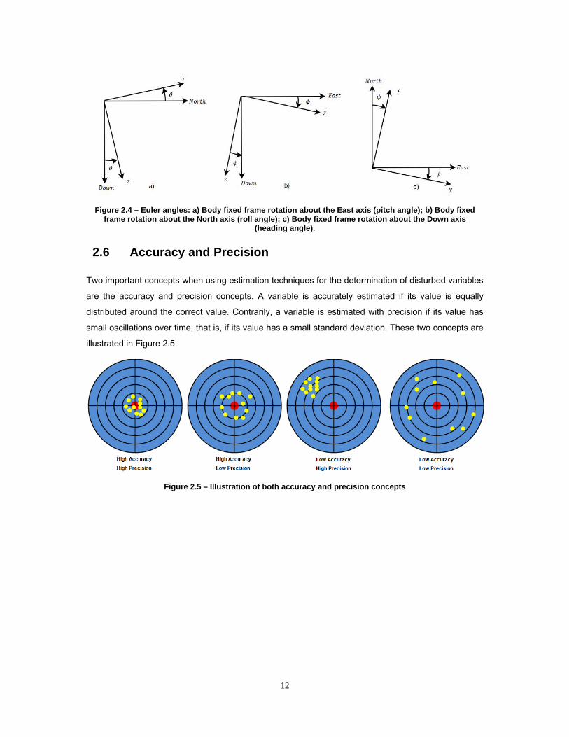
Figure 2.4 – Euler angles: a) Body fixed frame rotation about the East axis (pitch angle); b) Body fixed frame rotation about the North axis (roll angle); c) Body fixed frame rotation about the Down axis
(heading angle).
2.6 Accuracy and Precision
Two important concepts when using estimation techniques for the determination of disturbed variables
are the accuracy and precision concepts. A variable is accurately estimated if its value is equally
distributed around the correct value. Contrarily, a variable is estimated with precision if its value has
small oscillations over time, that is, if its value has a small standard deviation. These two concepts are
illustrated in Figure 2.5.
Figure 2.5 – Illustration of both accuracy and precision concepts

13
3 BASELINE DETERMINATION AND INTEGER AMBIGUITY RESOLUTION
3.1 Introduction
The determination of the baseline vector is done by using interferometric techniques. This technique
consists on the differentiation of two receivers’ measurements. Thus, in the GPS case the
measurements at hand lead to both carrier phase and code (pseudoranges) double differences, which
are used as observations in the developed system. However, to use carrier phase measurements the
integer ambiguities must be determined. In this chapter the developed system and the techniques
used for the baseline determination are presented.
3.2 System Definition
3.2.1 Observables
Generation of both carrier-phase and code double differences is essential for the determination of the
baseline vector between two GPS antennas. The double differences allow the cancellation of the
receiver and satellite clock biases and great part of ionospheric propagation delay. Considering that
the distance between both antennas is small, when compared with the receiver-satellite distance, one
may assume that the elevation angle is the same for both receivers. Hence, the tropospheric
propagation delay will largely cancel as well.
The carrier phase measured, in meters, for satellite and receiver has the form
, (3.1)
where,
is the geometric distance between the satellite and the receiver (in meters);
is the carrier wavelength (in meters);
is the unknown integer ambiguity (in cycles);
is the speed of light in vacuum (meters per second);
and are the satellite and the receiver clock offset (in seconds), respectively;
and are the tropospheric and ionospheric delay (in seconds), respectively;
is unmodeled noise due to different factors (hardware, multipath).
The carrier phase integer ambiguity, , is kept constant within the receiver as long as the satellite is
continuously tracked.

14
Adding another receiver measurement (let the new receiver be ) and assuming that both phase
measurements Φ and Φ correspond to the same instant, it is possible to generate a single
difference by subtracting both measurements. That is, the single difference for phase measurements
(ΔΦ ) would have the form
Δ Δ Δ Δ Δ . (3.2)
Equation (3.2) proves the cancellation of the satellite clock bias and the tropospheric and ionospheric
delays, since they are common term between the two receivers. However, the receiver clock bias is
not cancelled by operation (3.2). This can be done by double differencing.
Adding a new satellite ( ) it is possible to generate a double difference. This is done by subtracting
two single differences, the first one relative to receivers , and satellite and the second one
relative to the same set of receivers but for satellite . That is,
∆ . (3.3)
As previously said, the formation of double differences the receiver clock bias now cancelled. In order
to use the carrier phase double differences it is necessary the integer ambiguity determination.
The same process can be applied to code measurements that are defined as
, (3.4)
and the code double difference generation is straightforward, based on the process presented above.
Thus, code double differences are given by
∆ . (3.5)
Despite unambiguous, code double differences are noisier when compared whit carrier phase double
differences. Accordingly with [3] and [1], the standard deviation of the error in code double differences
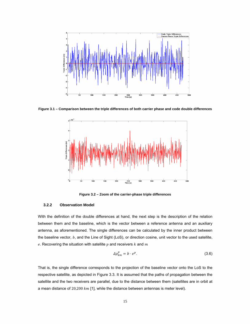
is meter level, while in the carrier phase double differences is centimeter level, as illustrated in Figure
3.1 where the triple differences, that consist in the differentiation through time and whose definition is
presented in the following sections, are used for comparison the precision levels between carrier
phase and code double differences. In Figure 3.2 is presented a zoom of the carrier-phase triple
differences depicted in Figure 3.1. Thus, for a precise baseline determination, one must make use of
carrier phase double differences and, consequently, calculate the integer ambiguities.
15
Figure 3.1 – Comparison between the triple differences of both carrier phase and code double differences
Figure 3.2 – Zoom of the carrier-phase triple differences
3.2.2 Observation Model
With the definition of the double differences at hand, the next step is the description of the relation
between them and the baseline, which is the vector between a reference antenna and an auxiliary
antenna, as aforementioned. The single differences can be calculated by the inner product between
the baseline vector, , and the Line of Sight (LoS), or direction cosine, unit vector to the used satellite,
. Recovering the situation with satellite and receivers and
⋅ . (3.6)
That is, the single difference corresponds to the projection of the baseline vector onto the LoS to the
respective satellite, as depicted in Figure 3.3. It is assumed that the paths of propagation between the
satellite and the two receivers are parallel, due to the distance between them (satellites are in orbit at
a mean distance of 20,200 [1], while the distance between antennas is meter level).

16
By differentiating equation (3.6) for satellites and , the double difference obtained would have the
form
∆ ⋅ ⋅ . (3.7)
The determination of the direction cosines and , which are assumed to be equal for both
receivers due to the big difference between the baseline length and the satellite-receiver distance, is
done by computing the user position and the respective satellite position.
Figure 3.3 – GPS interferometer for one satellite [1]
Combining (3.3) and (3.5) with (3.7), and expanding to a case with satellites, one would obtain the
system
∆∆⋮
∆∆∆⋮
∆
⋮ ⋮ ⋮
⋮ ⋮ ⋮
0 0 ⋯ 00 0 ⋯ 0⋮ ⋮ ⋱ ⋮0 0 … 0
0 … 00 … 0⋮ ⋮ ⋱ ⋮0 0 0
∆∆⋮
∆
⋮
⋮
. (3.8)
Note that the superscript 1 present in all differential terms is relative to the reference satellite, which is
the one with highest elevation. This definition of reference satellite is in order to maximize the
constellation geometry and stability.
The system (3.8) can be reduced to the form
, (3.9)
in which the subscript in each matrix represents its dimension and,

17
is the measured double differences’ vector;
is the system matrix for the baseline coordinates, containing the differenced direction
cosines;
is the baseline coordinates’ vector;
is the system matrix for the ambiguity set, containing the carrier wavelength;
is the aforementioned ambiguity set;
is the measurement noise vector.
Defining the augmented system matrix , with dimension 2 1 1 3 , one
would have an augmented state vector , with dimension 1 3 1. Analyzing the
augmented system is possible to conclude that there are enough equations to estimate all the states
(i.e. baseline vector coordinates and the double differences integer ambiguities), if the full rank of the
augmented system matrix is equal to the number of states, that is, equal to 1 3 . This
equality is only verified when the constellation has, at least, four satellites, that is for 4.
To use the system defined above, one must define the covariance matrix of the measurement error, ,
which is the next step of this thesis.
3.2.3 Observables Covariance
Both carrier phase and code measurements’ noise is assumed to be Gaussian distributed, with
expected value zero and variance and , respectively and assumed to be equal for all satellites.
Considering that measurements from different satellites are independent, this entails that those
measurements are uncorrelated. Hence, for a generic set of measurements, given by the column
vector and with the disturbance column vector , distributed like code and carrier phase (with
expected value zero and variance ), the respective covariance matrix is defined by,
, (3.10)
for a constellation with satellites and where represents the identity matrix.
By the definition of single difference, as shown in equation (3.2) for receivers and (which for each
satellite leads to measurement error Δ ), the derivation of the corresponding covariance
matrix is straightforward
2 . (3.11)

18
Equation (3.11) results in a diagonal matrix and this shows that the single differences are
uncorrelated.
As showed in the two previous sections, double differences are formed by the difference between the
single difference of the reference satellite and the single difference of the other satellites. Thus, the
double differences’ vector, for satellites, is given by
(3.12)
where
1 1 0 … 01 0 1 … 0⋮ ⋮ ⋮ ⋱ 01 0 0 … 1
. Finally, it is possible to determinate the double differences’
covariance matrix
2
2
2 1 … 11 2 … 1⋮ ⋮ ⋱ ⋮1 1 1 2
.
(3.13)
Thus, one may conclude that the double differences are correlated, which is evident since all double
differences are generated for the same reference satellite.
To conclude, both carrier phase and code double differences have the following covariance matrices,
correspondingly,
2 , (3.14)
2 . (3.15)
3.3 Integer Ambiguity Resolution
The system defined in (3.9) can be solved by a weighted least squares algorithm. From [6] it is known
that the usual problem in WLS is to minimize the error norm of the type ‖ ‖ , that is
, ‖ ‖ , (3.16)
where is the weight matrix.
The minimization gives floating point solutions that are highly contaminated by code’s noise and we
know that the correct ambiguities are integers, which is called the fixed solution. Such estimates are
called float solutions. This noisy solution can be improved by smoothing code double differences. The
correct integer ambiguities can be determined by search techniques that make use of the float
solution. All these tools will be better explained in next subsections.

19
3.3.1 Float Solution
As aforementioned, the system (3.9) can be solved by a weighted least squares estimator. For a
generic system , the estimator is given by, [6],
. (3.17)
Remembering the notion of augmented system introduced before, where and
, the estimator (3.17) can be applied to the problem at hand. The weight matrix is given
by the inverse of the measurements covariance matrices (3.14) and (3.15), that is
00
. (3.18)
Thus, our estimator should have the form
. (3.19)
It is important to obtain the float solution estimation’s covariance matrix, since it will have an important
role on fixed solution determination. Defining the estimation error as and using some
mathematical manipulation, one should obtain
, (3.20)
where represents the double differences’ noise with covariance matrix , as defined above. The
covariance matrix for the estimation error can be calculated from (3.20) with the form
. (3.21)
3.3.2 Code Smoothing
In this section, a code smoothing technique to improve the accuracy of the float solution is presented.
But for a better comprehension of this technique, the Kalman Filter will be briefly described.
Kalman Filter
The Kalman Filter (KF), introduced by [25], is a recursive mathematical model to estimate the state of
a system minimizing the mean of the squared error. In a first step, the filter “predicts” the system’s
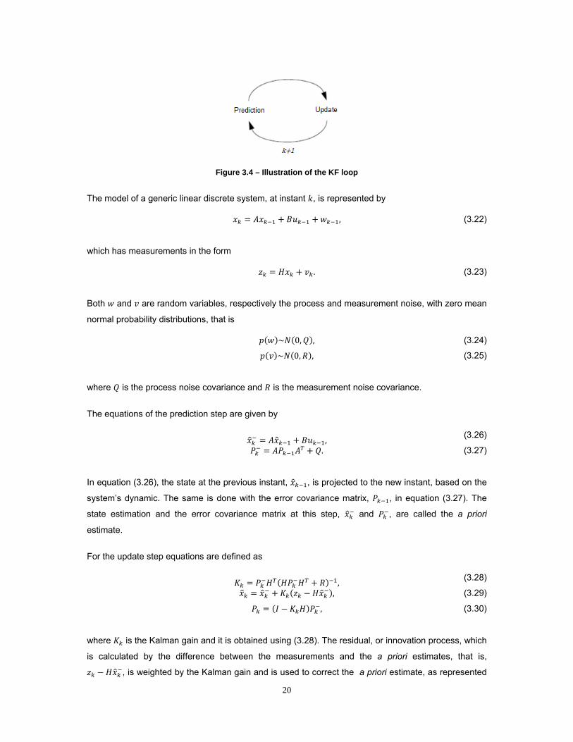
state in that instant, and then in a second step using a feedback control, based on the noisy
measurements, the filter “updates” the system’s state. Thus, two different steps constitute the KF: the
prediction step, and the update step, as depicted in Figure 3.4.
20
Figure 3.4 – Illustration of the KF loop
The model of a generic linear discrete system, at instant , is represented by
, (3.22)
which has measurements in the form
. (3.23)
Both and are random variables, respectively the process and measurement noise, with zero mean
normal probability distributions, that is
~ 0, , (3.24)
~ 0, , (3.25)
where is the process noise covariance and is the measurement noise covariance.
The equations of the prediction step are given by
,
(3.26)
. (3.27)
In equation (3.26), the state at the previous instant, , is projected to the new instant, based on the
system’s dynamic. The same is done with the error covariance matrix, , in equation (3.27). The
state estimation and the error covariance matrix at this step, and , are called the a priori
estimate.
For the update step equations are defined as
,
(3.28)
, (3.29)
, (3.30)
where is the Kalman gain and it is obtained using (3.28). The residual, or innovation process, which
is calculated by the difference between the measurements and the a priori estimates, that is,
, is weighted by the Kalman gain and is used to correct the a priori estimate, as represented
21
in equation (3.29). In equation (3.30) the new error covariance matrix is obtained. Note that the term
is the identity matrix. After these two steps, the process is repeated for a new instant, 1, using the
previous estimated state, , and the estimation covariance matrix, , as inputs for the new prediction
step.
For linear systems, the KF ensures stability, reachability and observability, and converges to the
optimal solution, [26] and [27]. However, for non-linear systems the direct application of the algorithm
presented above is not possible. The estimation for non-linear systems will be addressed during this
thesis.
Complementary Kalman Filter
Based on the KF, described in the previous section, the reader is now presented with the technique
used for code smoothing. This technique, used by [28], makes use of the combination between the
noisy code double differences and the less noisy carrier phase double differences with a
Complementary Kalman Filter. The technique uses the average of the noisier measurement to center
the quieter one, limiting the size of the integer ambiguity. Thus, the filter’s output, at instant, , is a
smoothed (less noisier) code double difference, ∆ .
For that, the filter has the form
∆ ∆ ∆ ∆ , (3.31)
∆ , (3.32)
∆ , (3.33)
∆ ∆ ∆ ∆ , (3.34)
. (3.35)
The first two lines (equations (3.31) and (3.32)) compose the prediction step. In the first one, the
smoothed code double differences are propagated from the previous instant with the change rate of
the carrier phase double differences. By differencing two carrier phase double differences, the integer
ambiguity is canceled, hence the propagated ∆ is unambiguous. In the second line, the error
covariance matrix is obtained by adding the new covariance matrix of the carrier phase measurements
to the previous error covariance.
For the update step, the Kalman gain is calculated as described in equation (3.33). In equation (3.34),
the predicted smoothed code double differences are propagated with the weighted residual between
the measured code double differences and the smoothed code double differences. Finally, in equation
(3.35) the estimation error covariance is propagated to the new instant, maintaining the balance
between the unambiguous but noisier code measurements and the ambiguous but smoother carrier
phase measurements.

22
3.3.3 LAMBDA Method
As aforementioned, the LAMBDA method was chosen as the search technique to use in this thesis
and it will be presented in detail. It has three steps: float solution, integer ambiguity estimation, and
fixed solution, [29].
The float solution step consists in the initialization of the LAMBDA method. The inaccurate solution
obtained by the weighted least squares estimator, in equation (3.19), is used in the search process
as the central point. The error estimation covariance, , defines the search space to finding the
correct integer ambiguity vector, , that minimizes the cost function,
∈ ‖ ‖ , (3.36)
that is the integer ambiguity estimation step.
Note that, the float solution obtained using the code smoothing technique, instead of the unsmoothed
float solution, could be used as an input in the LAMBDA method. However, it was decided to use the
unsmoothed float solution as an input rather than the smoothed float solution, which is only used as
comparison in the results section
The correlated nature of double differences leads to a non diagonal covariance matrix, as depicted in
the derivation of (3.13), which entails that the covariance matrix of the float solution is also not
diagonal, leading to an elliptical search space. This means that the search space can be more
elongated in one direction than in another, which results in integer ambiguity sets that have lower
values of the cost function but appear much farther away than those which appear nearby but are
outside of the search space. To fix this issue, the LAMBDA method uses a transformation matrix to
decorrelate the error and, therefore, diagonalizing (as much as possible, where the non diagonal
elements are close to zero) the covariance matrix of the float solution. This process will create a
search space that is nearly spherical, leading to an easier and faster search process.
This diagonalization process is accomplished by a transformation defined as
, (3.37)
where both and must have integer entries, so that the original and the transformed ambiguities
remain integer.
Next, the covariance matrix of the float solution can be decomposed as
, (3.38)
where is a lower matrix and is a diagonal matrix. Assuming that is close to one must have

23
, (3.39)
where the non diagonal elements of this new covariance matrix, represented by , are close to zero,
leading to a nearly diagonal covariance matrix.
After the transformation and the decorrelation process, the new cost function is defined as
‖ ‖ , (3.40)
where and .
The volume of the search space is controlled by the value , that is constant during the search
process and takes into account the new nearly diagonal covariance matrix and the number of
candidates desired by the user. That is, the LAMBDA method outputs those ambiguities that verify the
inequality
. (3.41)
The number of candidates selected by the user must consider the distance between the float solution
and the true integer solution, and the computation time available. That is, a number of candidates too
small could lead to a solution that do not include the true integer solution and a number of candidates
too big won’t permit the adaptation to real-time applications. A study on the influence of the number of
candidates is presented in [8].
At the end of the LAMBDA method, the required number of candidates is transformed back to the
initial form, resorting to
, (3.42)
where the solution remains integer, due to the aforementioned nature of and . Note that the
candidates outputted from the LAMBDA method are sorted in ascending order of the distance to the
float solution.
3.3.4 Ambiguity Filter
Following the methodology developed in [8], the Ambiguity Filter developed in this thesis chooses the
best integer ambiguity set from LAMBDA method’s output. For each candidate set , as resulting from
LAMBDA method, the corresponding baseline, , is computed with the objective of attributing merit
to each candidate. For that, the developed method has three steps: validation, selection and
stabilization. Before the description of these three steps, the tests used in this thesis for merit
attribution are presented.
24
Merit Attribution
In merit attribution were used three types of metrics. The first two, also present in [8], were the
residual ratio and the baseline length constraint. The third one, proposed in this thesis, makes use of
the Up coordinate while the ambiguity set is not stabilized.
The residual ratio: for each ambiguity set and the respective baseline solution, the phase residual
vector is calculated as the difference between the estimated phase double differences and the
measured ones. That is, the phase residual vector is given by
∆ , (3.43)
and its Euclidean norm is obtained by
‖ ‖ ΔΦ . (3.44)
The baseline length constraint: with the knowledge of the truth baseline distance, , the error of the
estimated baseline is obtained as
. (3.45)
The Up coordinate constraint: this test is similar to the previous one, but only considers the Up
coordinate resulting from the candidate set that is being tested. It is assumed that during the
initialization (i.e. while there is no stabilized solution) the platform is stopped, which leads to a constant
baseline vector. By measuring the altitude difference between the reference antenna and the auxiliary
antenna, it is possible to obtain the real Up coordinate, . Thus, the Up coordinate error is given by
| |. (3.46)
For each of the three tests defined above, the errors of the candidates are grouped in a vector with
ascending order of the respective error, which is the descending order of merit. So, the merit, , of a
candidate set will be attributed according with the position, , of the error in the sorted vector, that is
1. (3.47)
Validation Step
The validation step makes use of the baseline length error, described in (3.45), and defining a
threshold. This threshold was set to be 10 , due to the nature of the errors present in the baseline
vector. That is,
0.1. (3.48)

25
The candidates that have a baseline length error bigger than the threshold are excluded.
Selection Step
This step is where the merit is attributed. This is done by combining two of the tests defined previously
in two different metrics:
1. Residual ratio and baseline length constraint;
2. Baseline length constraint and Up coordinate constraint.
The candidate set with higher merit, using the metric 1 or the metric 2, will be selected as the fixed
solution for the respective epoch.
Stabilization Step
The candidate set selected as the fixed solution by the Ambiguity Filter in each epoch is stored in a
data base. As debated in [8], the ambiguity set that first achieves 50 occurrences as the fixed solution
(i.e. a candidate is selected as the fixed solution in 50 different epochs) is the correct fixed solution.
Thereafter the correct baseline vector will be determined by the best fixed solution.
In dynamic environments variations in the satellite constellation occur quite often (i.e. change of the
reference satellite, loss of lock, cycle slips), that entails to the lost of the correct ambiguity set. The
algorithm proposed in this thesis uses the same constellation in the maximum number of epochs.
Even if a new satellite becomes visible, the algorithm uses those satellites for which the correct integer
ambiguity set is known. When the number of satellites falls to less than four, the algorithm uses the
last baseline’s estimate (i.e. calculated using the correct ambiguity set) and recovers the correct
ambiguity set for the new constellation. Then the recovered ambiguity set is used to calculate the
present baseline vector. This adaptation to a new constellation represents an improvement in the use
of the Ambiguity Filter and the techniques used will be presented next. If neither of the recovery
techniques is capable of maintaining the integer ambiguity solution, the Ambiguity Filter must be
reinitialized and start the process from the beginning.
3.3.5 Constellation Changes: Recovery Techniques
As said before, constellation changes lead to the loss of both correct ambiguity set, obtained after
stabilization, and the ambiguities stored through the different epochs. However, some techniques can
be used to recover from this scenario, without resetting the system.
Reference Satellite Transformation
As aforementioned, the reference satellite is the one with highest elevation. However, during the
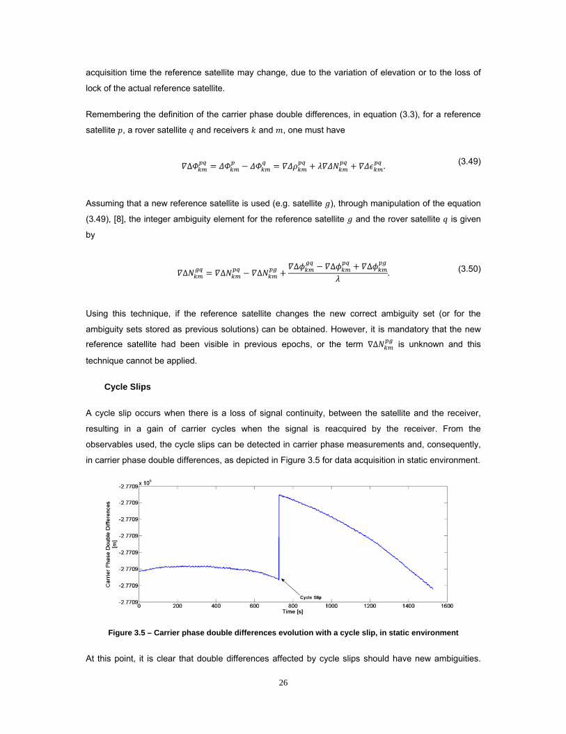
26
acquisition time the reference satellite may change, due to the variation of elevation or to the loss of
lock of the actual reference satellite.
Remembering the definition of the carrier phase double differences, in equation (3.3), for a reference
satellite , a rover satellite and receivers and , one must have
∆ . (3.49)
Assuming that a new reference satellite is used (e.g. satellite ), through manipulation of the equation
(3.49), [8], the integer ambiguity element for the reference satellite and the rover satellite is given
by
∆ ∆ ∆∆ ∆ ∆
. (3.50)
Using this technique, if the reference satellite changes the new correct ambiguity set (or for the
ambiguity sets stored as previous solutions) can be obtained. However, it is mandatory that the new
reference satellite had been visible in previous epochs, or the term ∆ is unknown and this
technique cannot be applied.
Cycle Slips
A cycle slip occurs when there is a loss of signal continuity, between the satellite and the receiver,
resulting in a gain of carrier cycles when the signal is reacquired by the receiver. From the
observables used, the cycle slips can be detected in carrier phase measurements and, consequently,
in carrier phase double differences, as depicted in Figure 3.5 for data acquisition in static environment.
Figure 3.5 – Carrier phase double differences evolution with a cycle slip, in static environment
At this point, it is clear that double differences affected by cycle slips should have new ambiguities.
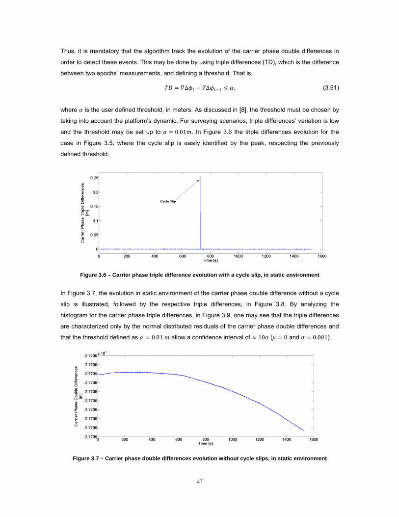
27
Thus, it is mandatory that the algorithm track the evolution of the carrier phase double differences in
order to detect these events. This may be done by using triple differences (TD), which is the difference
between two epochs’ measurements, and defining a threshold. That is,
∆ ∆ , (3.51)
where is the user defined threshold, in meters. As discussed in [8], the threshold must be chosen by
taking into account the platform’s dynamic. For surveying scenarios, triple differences’ variation is low
and the threshold may be set up to 0.01 . In Figure 3.6 the triple differences evolution for the
case in Figure 3.5, where the cycle slip is easily identified by the peak, respecting the previously
defined threshold.
Figure 3.6 – Carrier phase triple difference evolution with a cycle slip, in static environment
In Figure 3.7, the evolution in static environment of the carrier phase double difference without a cycle
slip is illustrated, followed by the respective triple differences, in Figure 3.8. By analyzing the
histogram for the carrier phase triple differences, in Figure 3.9, one may see that the triple differences
are characterized only by the normal distributed residuals of the carrier phase double differences and
that the threshold defined as 0.01 allow a confidence interval of 10 ( 0 and 0.001).
Figure 3.7 – Carrier phase double differences evolution without cycle slips, in static environment

28
Figure 3.8 – Carrier phase triple differences evolution without cycle slips, in static environment
Figure 3.9 – Histogram of triple differences without cycle slips, in static environment
As described in [8], the worst scenario is the type of movement with high angular velocities, which
imposes a sinusoidal evolution to the double differences, that is,
∆ , (3.52)
where is the baseline length and is the maximum angular velocity of the vehicle. Thus from the
conclusions described in [8], the maximum value for the TD in this type of scenario is function of the
baseline length and the vehicle’s angular velocity, that is,
22
. (3.53)
Since the dynamic trials were performed with slow movements, a small value for the vehicle’s angular
velocity ( 0.5 / ) was considered. However, improvements in the estimation of the vehicle’s
angular velocity could be addressed, in order to validate this technique for different dynamics.
When a cycle slip is detected in an explicit double difference, the stored integer ambiguities and the
correct integer ambiguity, if known, must be corrected. In this thesis, the recovery of an ambiguity set

29
from a cycle slip is done by adding the rounded triple difference to the previous integer ambiguity. That
is,
∆ ∆ . (3.54)
Variation in the Number of Satellites
During the data acquisition in real environments the number of satellites used to compute the baseline
vector changes quite often, due to the loss of signal or even loss of data in the interface. Instead of
resetting the Ambiguity Filter, the algorithm deletes the ambiguity component relative to the lost
satellite and keeps tracking the remaining satellites with the previously obtained ambiguities.
As aforementioned, the algorithm uses the same satellites as much as possible, so that the stability is
maximized, that is, even if a new satellite becomes visible the algorithm uses the satellites for which
the correct ambiguities are known.
When the number of used satellites falls to less than four, the algorithm uses the last estimation of the
baseline vector to estimate the ambiguity set for all visible satellites, that is, from (3.19) one may
obtain
∆ , (3.55)
where is the last baseline’s estimation. It is assumed that between two epochs the baseline vector
has small changes and can be used to estimate the new ambiguity set.

30

31
4 ATTITUDE DETERMINATION
4.1 Introduction
The configuration of multiple baselines allows the attitude determination. By using the Ambiguity Filter,
described in the previous chapter, for baseline determination, two techniques for attitude
determination are proposed.
With the definition of the Euler angles presented in the Chapter 2 in mind, two techniques for the
attitude determination are presented. First, a simple technique using rotation matrices is presented.
Finally, a more complex solution using a rotation quaternion and a generalization of the Kalman Filter
(KF) is proposed.
4.2 Attitude Determination Using a Rotation Matrix
As discussed in [1] and in [28], among other possible solutions assume that the attitude is defined by
the rotation transformation which relates a coordinate frame fixed in space NED to a coordinate frame
fixed in the body ( ). Due to its nature, the coordinates of the baselines will be constant in the body
frame and are known.
The rotation of the body fixed frame can be represented as a series of rotations from the body fixed
frame to the reference space frame. First a rotation about the axis (angle ), followed by a rotation
about the new axis (angle ) and , finally, a rotation about the newest axis (angle ). That is,
, , , (4.1)
where each rotation matrix is a 3 3 square matrix and with | | | | 1
The resulting rotation matrix, also a 3 3 square matrix and with | , , | 1, is represented
by
, , ⋯
cos cossin cos
cos sin sinsin sin
cos sin cos
sin coscos cos
sin sin sincos sin
sin sin cossin cos sin cos cos
.
(4.2)
The transformation from the body fixed frame to the space frame is given by

32
, , , (4.3)
where | … |
…| ⋯ |
and
| … |…
| ⋯ | are matrices of baselines (as columns) in
the respective coordinate frame.
Thus, using the baselines vectors, in the space frame, calculated in each epoch, the rotation matrix at
each epoch may be calculated by solving as a simple Least Squares (LS) problem, that is
, , . (4.4)
After the determination of the rotation matrix, one may obtain the attitude angles using simple
trigonometric relations, as represented next
, (4.5)
cos ,
(4.6)
cos ,
(4.7)
where the subscript in the rotation matrix represents its index. The expressions for the pitch and roll
angles (equations and (4.6), respectively) assume a rotation between 2⁄ ; 2⁄ , and the
expression for the heading angle (equation (4.7)) assume a rotation between 0; , thus one cannot
have all possible orientations. To correct this issue, depending on the signal of the baselines’
coordinates the attitude angles must be corrected to the real quadrant.
This approach has singularities for pitch angles of 2⁄ . However, it is easy to obtain the attitude
angles for situations where such attitude is not experienced. For a more robust and stable
implementation, a rotation quaternion may be used.

33
4.3 Quaternion-Based Extended Kalman Filter for Attitude Determination
4.3.1 Quaternion and Euler Angles
As described in [30], instead of rotation matrices, a quaternion may be used as rotation operator. A
quaternion is a hyper-complex number of rank 4, and it is defined as
, (4.8)
where is called the scalar part and are called the vector part.
The computation of a baseline vector in the coordinate frame NED from the Body fixed frame, in terms
of a rotation quaternion, is given by
∗ , (4.9)
where ∗ represents the complex conjugate of the quaternion . An important
property is that the quaternion is a unit vector, that is
‖ ‖ 1, (4.10)
which consists in a crucial constraint when using a quaternion for attitude determination, as presented
in the development of the Extended Kalman Filter (EKF) proposed in next section.
Thus, the rotation matrix , in terms of quaternions is represented by
1 2 2 22 1 2 22 2 1 2
.
By substituting the matrix , , with the quaternion matrix, , equation should have the new
form
. (4.11)
The Euler angles can be obtained from the quaternion matrix as
, (4.12)
34
,
(4.13)
,
(4.14)
where the superscript in the matrix represents its index.
4.3.2 Extended Kalman Filter
Instead of the LS presented in Section 4.2, which provide an epoch-by-epoch solution, the KF allow
better results since it is a recursive estimation algorithm. However, with the observables at hand it is
not possible to apply the linear KF due to the measurement model, as depicted during this section.
To obtain the Euler angles based on the rotation quaternion it is necessary to estimate the parameters
, , and . The system dynamics of the quaternion is represented by
12Ω , (4.15)
where is the vector with the quaternion components, that is, , and Ω is the skew-
symmetric matrix, defined as
Ω
00
00
, (4.16)
where are the angular velocities in the body frame axis. The observations of angular
velocities may be provided by a rate gyro. However, in this thesis only GPS observables and its
derivations are used as observations. Thus, the angular velocities must be estimated along with the
quaternion components. It is assumed a constant angular velocity model, which is a good
approximation for a short measurement interval and for a vehicle with low dynamics, [31], with the
disturbances being interpreted as inputs to the system.

35
So, this leads to a linear time-varying discrete system defined as
, (4.17)
with each component being
,
(4.18)
12Δ Ω , (4.19)
12Ξ 0
0,
(4.20)
Ξ ,
(4.21)
where Δ is the sampling time (Δ 1 for the GPS case), is the process noise, Gaussian
distributed with zero mean and covariance , and Ξ Ω , accordingly with [32].
By using the baselines’ coordinates, from the previously presented Ambiguity Filter, as
measurements, the relation between measurements and the system’s sate vector is given by equation
(4.11). In addition, the measurement model takes into account the constraint imposed by the
quaternion nature, which is a unit vector as represented in equation (4.10). This is done by using this
constraint as a perfect measurement, as described in [27]. So, the measurement model is non linear
time-varying and has the form
, (4.22)
where is the measurement noise, Gaussian distributed with zero mean and covariance , and
1
, (4.23)
36
.
(4.24)
Since the system model is linear time-varying and the observation model is non linear time-varying, to
estimate the quaternion components and the angular velocities it is necessary to implement an EKF.
The EKF consists in the system’s linearization around the nominal solution that results from the KF
estimation.
Thus with the system at hand, it is mandatory the linearization of the measurement model. This is
done by Taylor Series expansions, where neglecting the high order terms (assumed to have small
numeric value), [33], leads to the Jacobian matrix defined as
.
(4.25)
The process noise characterizes the small disturbance in the system’s dynamics and is given by, [33]
and [34],
, , , (4.26)
where , accordingly with [32], is a diagonal matrix and containing the covariance of the disturbances
present in the angular velocities, that is,
0
0 , (4.27)
where is the covariance of the angular velocity noise and is the covariance of the angular
velocity bias noise. These two parameters must be tuned in order to obtain the best solution, but since
it is not used any rate gyro, it is assumed that the value of is close to zero.
To solve the equation (4.26), in order to obtain the process covariance matrix, it is assumed that the
time interval between two measurements (1 for the GPS) is small enough to use the approximation
∆ . (4.28)

37
Since the measurements used are the coordinates of the baseline vectors (assumed to be
independent), the measurement covariance matrix is diagonal with each component regarding the
corresponding coordinate, that is for a single baseline observation one must have
0 0
0 00 0
. (4.29)
Thus, for three baselines and the quaternion-norm perfect measurement, the observation covariance
matrix of the EKF is defined as
0 0 0
0 0 00 0 00 0 0 0
. (4.30)
Finally, the EKF should have the form
,
(4.31)
. (4.32)
,
(4.33)
, (4.34)
. (4.35)
where, as previously described, the first two lines are the prediction step, where the state vector and
the respective covariance matrix, estimated in the previous instant, are propagated to the new time
step. The remaining lines correspond to the update step, where the Kalman gain is determined and is
used to weight the state prediction, based on the innovation process given by the difference between
the measured baseline vectors and the ones obtained from the estimated quaternion, .
This innovation process is used in the results section as a tool to evaluate the performance of the
EKF.
Instead of the linear KF, the EKF solution is optimal only around the linearization nominal point and
the conditions for stability are not necessarily sufficient. The stability in non-linear systems is possible
only inside bounded regions, [27] and [33]. The reachability and observability will be addressed in next
section.
4.3.3 Reachability and Observability
The concept of reachability for a discrete-time system, which is analogous to controllability for a
continuous-time system, defines how well the system is reachable (or controllable). Thus, accordingly
38
with [27], a discrete-time system is reachable if for any initial state and some final time there
exists a control that transfers the state to any desired value at time .
Accordingly with [35], this may be verified by the rank of the reachability matrix, which for the system
defined in the previous section and for the time interval , is defined by
, 1 , 1 2 … , 1 . (4.36)
That is, the linear time-varying system by (4.17), with state variables, is reachable on the time
interval , , if and only if the reachability matrix verifies
, . (4.37)
The next important concept is the observability, that relates how well it is possible to determinate the
initial conditions through the observations. Thus, accordingly with [27], a discrete-time system is
observable if for any initial state and some final time , the initial state can be uniquely determined
by the corresponding zero-input response .
Accordingly with [35], this may be verified by the rank of the observability matrix, which for the system
at hand and for the time interval , is defined by
,1 1,
⋮1 1,
. (4.38)
That is, the linear time-varying system by (4.17), with state variables, is observable on the time
interval , , if and only if the observability matrix verifies
, . (4.39)
In the system (4.17) the state variables are the quaternion elements and the angular velocities
components, thus it is a system with 7 state variables. By computing the desired matrices for
formation of both reachability and observability matrices, in a significant time interval, it was possible
to verify that the conditions for reachability and observability were respected, that is,
, 7, (4.40)

39
, 7.
(4.41)
Finally, based on the results of (4.40) and (4.41), it is possible to conclude that the EKF implemented
can provide a solution for the problem at hand and is unique.

40

41
5 SOLUTION IMPLEMENTATION
5.1 Introduction
After the description of the tools used to solve the problem of the attitude determination using multiple
baselines, and how to determine those baselines, this section addresses the practical issues of this
thesis. Two types of GPS receivers were used: Magellan AC12 and U-Blox 6. Thus, it is important to
introduce a general description for both receivers and the antennas used. Following the receivers’
introduction, a description of the developed algorithm, using the previously discussed tools, is
presented. Finally, the reader is presented with the description of the trials, static and dynamic, used
to validate the developed algorithm.
5.2 GPS Receivers and Antennas
5.2.1 Magellan AC12 GPS Receivers
In order to have a three baselines system, four Magellan AC12 GPS receivers were used, two
evaluation and development kits and two OEM boards as illustrated in Figure 5.1, [36], respectively.
Figure 5.1 – a) AC12 sensor evaluation and development kit; b) AC12 OEM board [36]
The receiver processes signals, on the L1 frequency band, from the GPS satellite constellation, for
which uses ten channels, and SBAS, in two channels, leading to a total of twelve signal tracking
channels. The receiver provides real-time position, velocity, and time measurement, amongst other
significant information, in NMEA format. The receiver also provides the satellites ephemeris, which are
essential for the development of single positioning algorithms, through a binary message. However,
this receiver does not provide the ionospheric correction parameters, which allow an improvement on
the single positioning. Regarding the double differences computation, the AC12 receiver provides a
binary message containing both carrier phase and code raw measurements. The communication with
the receiver is made with RS-232 interface.

42
5.2.2 U-Blox 6 GPS Receivers
The single positioning of the reference antenna is part of the developed algorithm. In order to improve
the positioning accuracy, one may use the ionospheric parameters to correct the code measurements.
Since the Magellan AC12 receivers do not provide such parameters, one U-Blox 6 GPS receiver,
illustrated in Figure 5.2, was used for this purpose, [37]. As for the AC12, the U-Blox provides real-
time positioning, velocity, and time measurements, amongst other significant information, through
NMEA messages, and binary messages containing raw measurements, satellite ephemeris and
ionospheric corrections, and along with other important information.
Figure 5.2 – U-Blox 6 GPS receiver [37]
The reader may ask why not use only U-Blox receivers. However, the performance of the Ambiguity
Filter, using these receivers, was lower than the performance when using AC12 receivers. For this
reason, it was decided to adopt the described set of GPS receivers.
The communications with the receiver is made using the RS-232 interface and through USB
connection.
5.2.3 Antennas
For the Magellan AC12 GPS receivers presented above, three types of antennas were used. For static
(or survey) tests with two GPS receivers, two Novatel model 531 GPS antennas with Chocke Ring
model A032 [38], depicted in Figure 5.3. This type of antenna operates at the L1 frequency. Antenna
optimization in the shape of the radiation pattern along with the Chocke Ring allows the minimization
of multipath and interference errors.
Figure 5.3 – Novatel model 531 GPS antenna with Chocke Ring Model A032 [38]

43
For multiple baselines (more than two receivers) in static and dynamic trials, the AC12 receivers used
a NAIS Magnetic antenna, [36], illustrated in Figure 5.4. Smaller than the previous antenna, allow
more versatility in the set up. However, is subject to higher levels of interference and multipath errors.
Figure 5.4 – NAIS magnetic antenna [36]
Finally, the U-Blox 6 receiver uses an ANN-MS-0-005 magnetic antenna, [39], which is similar to the
NAIS magnetic antenna depicted in Figure 5.4.
5.3 Algorithm Overview
Using the techniques presented so far in this thesis, the algorithm illustrated by the flowchart of Figure
5.3 was developed in MatLab. Note that the data acquisition of the GPS measurements was done
previously and then inputted to the algorithm in post-processing mode. So, the first process with the
name “Data Acquisition” regards the acquisition of the raw data previously stored. However, this
program could be adapted in order to use data in real time, being the “Data Acquisition” process
responsible for reading the measurements provided by the GPS receiver. With the data at hand, it is
mandatory that measurements from different receivers are synchronized, which is done by the “Data
Synchronization” process. This is done by comparing the measured time of week of each receiver,
which represents the number of seconds passed since the beginning of the corresponding week
(beginning at Saturday/Sunday midnight).
To determine the baseline vector coordinates it is mandatory to know the origin of the local coordinate
system (ENU or NED) in the ECEF coordinate system, which coincides with the position of the
reference antenna. This is done in the “Reference Antenna Stand-Alone Positioning” process,
resorting to code measurements, code corrections and satellite ephemeris, as described in [21]. The
“Double Differences Formation” process is responsible for the selecting satellites, common to the
receivers that compose the baseline vector, and computing the double differences. For the satellite
selection process an elevation mask of 5° was used, which neglect noisier satellite measurements.

44
Figure 5.5 – Flowchart of the developed algorithm
After computing the double differences some tests must be accomplished. The first test is to verify of
there is any change in the number of satellites. If this test output the logic value “true”, the respective
algorithm correct this issue by excluding the ambiguity (from the correct ambiguity set and from the
stored ambiguities) corresponding to the lost satellite. After this correction, the flowchart converges
with the node that would be reached if the tested turned out “false”. The second test verifies if there is
a new reference satellite. If the output is the logic true, the transformation of equation (3.50) must be

45
applied. The last test that is applied to the double differences is the cycle slip verification. If a cycle slip
is detected, returning the logic true in the detection test, the respective correction is applied.
With the double differences accomplishing the previous tests, the algorithm determines the float
solution of both baseline vector and ambiguity set, in “Float Solution” process, by solving the WLS
defined in equation (3.19). An alternative float solution is obtained by smoothing the code double
differences using the respective algorithm, and then determining the corresponding float solution.
By using the non-smoothed float solution as an input, the LAMBDA method outputs the intended
number of candidates sorted by the distance from the float solution, as described in Section 3.3.3.
From these candidates, the Ambiguity Filter selects the one with highest merit/confidence as the
correct fixed ambiguity set, which is outlined in Section 3.3.4. The ambiguity set selected by the
Ambiguity Filter is then stored in a data base, where is verified if the correct solutions was already
achieved, which consists on the stabilization process of the Ambiguity Filter. If there is not an optimal
solution, the Algorithm proceeds to the next iteration from this point. However, if the optimal solution
was already achieved, the attitude angles are obtained resorting to one of the two methods presented
in Sections 4.3 and 4.4. After obtaining the attitude angles, the algorithm proceeds to the next
iteration.
Note that in multiple baseline scenarios, each vector is calculated separately and only in the attitude
determination step all the baselines are computed to obtain the Euler angles.
5.4 Trials Description
To validate the developed algorithm, static and dynamic trials were made. For the static trials, the first
type is a test using a single baseline (i.e. two GPS receivers), and the second type is a test using
three baselines (i.e. four GPS receivers). For the dynamic trials, the platform using multiple baselines
was in motion along a route.
5.4.1 Static Trials
Single Baseline
The objective of this first type of static test is the performance evaluation of the Ambiguity Filter. For
high accuracy in the baseline determination, minimizing the multipath effect, the Novatel 531 antennas
with Chocke Ring were used. These antennas are placed in the rooftop of the North Tower, at Instituto
Superior Técnico, as depicted in Figure 5.6, which allow a scenario with very low levels of multipath.
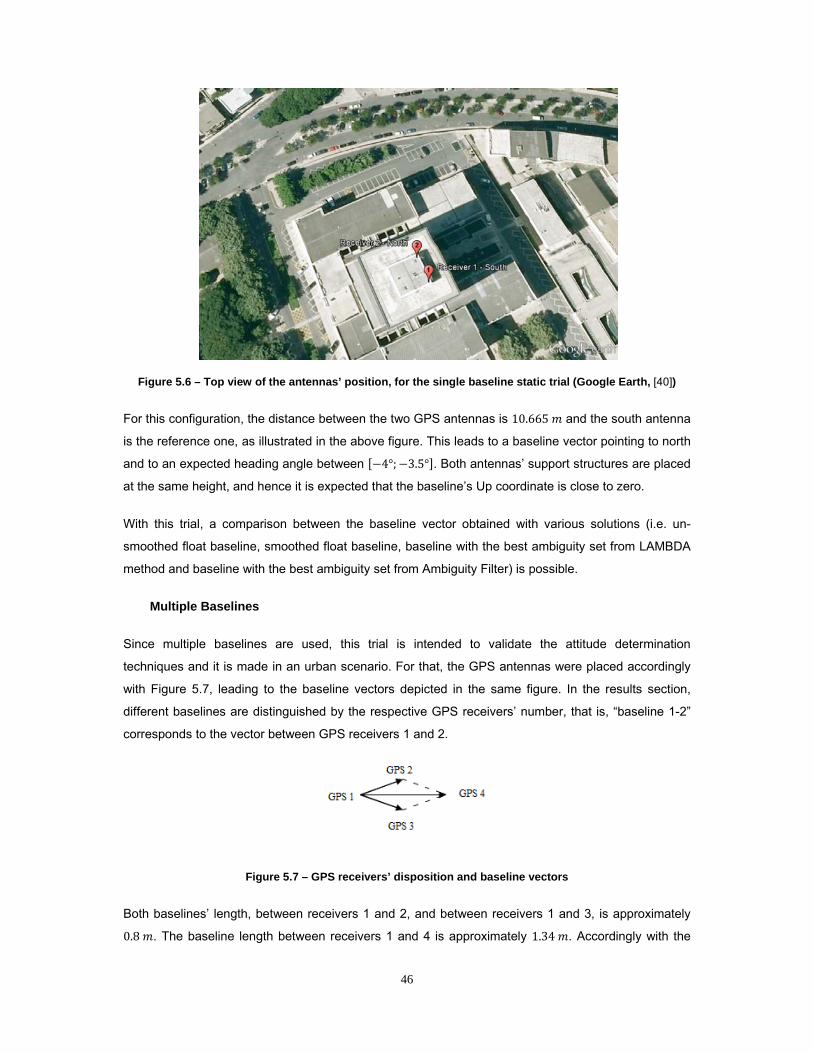
46
Figure 5.6 – Top view of the antennas’ position, for the single baseline static trial (Google Earth, [40])
For this configuration, the distance between the two GPS antennas is 10.665 and the south antenna
is the reference one, as illustrated in the above figure. This leads to a baseline vector pointing to north
and to an expected heading angle between 4°; 3.5° . Both antennas’ support structures are placed
at the same height, and hence it is expected that the baseline’s Up coordinate is close to zero.
With this trial, a comparison between the baseline vector obtained with various solutions (i.e. un-
smoothed float baseline, smoothed float baseline, baseline with the best ambiguity set from LAMBDA
method and baseline with the best ambiguity set from Ambiguity Filter) is possible.
Multiple Baselines
Since multiple baselines are used, this trial is intended to validate the attitude determination
techniques and it is made in an urban scenario. For that, the GPS antennas were placed accordingly
with Figure 5.7, leading to the baseline vectors depicted in the same figure. In the results section,
different baselines are distinguished by the respective GPS receivers’ number, that is, “baseline 1-2”
corresponds to the vector between GPS receivers 1 and 2.
Figure 5.7 – GPS receivers’ disposition and baseline vectors
Both baselines’ length, between receivers 1 and 2, and between receivers 1 and 3, is approximately
0.8 . The baseline length between receivers 1 and 4 is approximately 1.34 . Accordingly with the

47
studies presented in [11], these values for the baseline length allow high accuracy in the baseline
determination.
For this trial, four NAIS magnetic antennas were used. Since the data acquisition was made in an
urban scenario and the antennas used are more exposed to multipath, than the ones used in the
single baseline trial, it is expected to increase the multipath effect, when compared with the single
baseline test. The scenario in which the data acquisition took place and the platform’s orientation, with
an expected heading angle between 120°; 110° , are depicted in Figure 5.8. Since the platform
was stopped in a flat surface, it is expected that the Up coordinate of each baseline is close to zero.
Figure 5.8 – Top view of the platform’s orientation for the multiple baselines static trial (Google Earth, [40])
5.4.2 Dynamic Trial
This trial intended to evaluate the performance of the attitude determination techniques in a dynamic
environment, that is, for data acquired in a moving platform. The GPS receivers and the antennas’
disposition used were the same as presented in the previous section, that is, for the static trial in the
multiple baselines case. The platform was in motion along a flat surface and with considerable
variation on the heading angle, as depicted in Figure 5.9. The maneuvers made by the platform along
the trajectory were slow, so it is not excepted very aggressive angular velocities estimated by the EKF.
During the trajectory it was imposed to the platform a positive rotation about the axis, that is, a
positive roll angle. This test was made between epochs ∈ 235; 255 , when the platform’s heading
was 30°. Despite this test, the remaining variations in pitch and roll angles are due to surface
irregularities and multipath noise.

48
The orientation of the initial and the final position, as depicted in Figure 5.9, is expected to be between
30°; 20° and 115°; 110° , respectively.
Figure 5.9 – Top view of the platform’s path and orientation, for initial and final position, for the dynamic trial (Google Earth, [40])

49
6 RESULTS
6.1 Introduction
In this chapter the results from the trials previously described are presented. Along with the results, a
critical discussion is made to evaluate the performance of the developed techniques.
The single baseline static trial is used to evaluate the Ambiguity Filter performance, by analyzing the
corresponding baseline solution. This solution is compared with the one obtained from LAMBDA
method’s best candidate integer ambiguity set, with the float solution and with the smoothed version of
the float solution. This performance evaluation is done by comparing the evolution and the precision
levels given by the mean ( ) and standard deviation ( ) – with a confidence interval of 68.2%. The
same is done with pitch and heading angles, which can be determined with a single baseline
configuration.
In the multiple baseline static trial it is done the same performance evaluation made in the single
baseline case, for a more conclusive and robust evaluation of the developed techniques since the
scenario introduces higher disturbance levels. Along with the comparison between the different
techniques for baseline determination, the multiple baselines configuration allows the full
determination of the attitude angles. Thus the performance of the developed algorithms for attitude
determination is discussed. For the EKF, the respective innovation process, between the measured
baseline coordinates and the ones estimated based in the quaternion elements, and the estimated
angular velocities are analyzed.
Finally, the dynamic trial is analyzed in terms of the attitude angles’ performance. This is done by
comparing both attitude solutions, along with the performance of the EKF, that is given by the
innovation process and the performance of the estimated angular velocities.
6.2 Static Trials Results
6.2.1 Single Baseline Results
Ambiguity Filter Performance
The first exercise is the performance comparison between the Ambiguity Filter’s metrics. Using the
metric 1, taking into account the carrier-phase residual ratio and the knowledge of the baseline length,
or the metric 2, with the previous knowledge of the baseline Up coordinate in the place of the carrier-
phase residual ratio, the evolution of the baseline solution may be different. As depicted in Figure 6.1,
both metrics have different baseline lengths through time. While the baseline length of the solution
using metric 2, characterized by the red line, instantaneously converges to the correct solution, the
first metric’s solution, sketched by the blue line, takes more epochs to stabilize. However, both

50
solutions converge to the correct solution, despite the longer time needed by the first metric’s solution.
Figure 6.1 – Baseline length evolution, using the Ambiguity Filter’s metrics 1 and 2 to solve the integer ambiguity problem for the single baseline static trial
This is emphasized by the evolution of the baseline coordinates for both metrics, illustrated in Figure
6.2. As presented during the trials description, both GPS antennas are at the same height, and thus it
is expected that the correct solution is the one with an Up coordinate close to zero. Since the baseline
solution using the metric 2, again depicted by the red line, shows a better performance than the
solution using metric 1 (blue line), since converges faster to the correct solution (with the Up
coordinate being close to zero). In Figure 6.3 is presented a zoom of the baseline ENU coordinates
using metric 2. By analyzing it, along with the evolution of the number of visible satellites in Figure 6.4,
it is possible to verify that the baseline solution is not affected, despite the variation in the number of
visible satellites. This is possible due to technique developed to manage the stored ambiguity
candidates and the correct solution determined by the Ambiguity Filter.
Figure 6.2 – Baseline ENU coordinates evolution, using the Ambiguity Filter metrics 1 and 2 to solve the integer ambiguity problem for the single baseline static trial

51
Figure 6.3 – Zoom of the baseline ENU coordinates evolution, using the metric 2 of the Ambiguity Filter to solve the integer ambiguity problem for the single baseline static trial
Figure 6.4 – Number of satellites visible during the data acquisition in the single baseline static trial
Comparison between Ambiguity Filter, LAMBDA Method, Float Solution and Smoothed
Float Solution
At this point, it is important the comparison between the Ambiguity Filter’s solution, using the better
solution given by metric 2, with other techniques for the integer ambiguity resolution, as described in
this thesis. From Figure 6.5, where the evolution of the baseline length is depicted, and from Figure
6.6, where the evolution of the baseline ENU coordinates is illustrated, it is possible to verify that the
solution obtained from the LAMBDA method’s best candidate in this, method’s sense, and the float
solution are very similar. In fact, the float solution has better precision, which is proved by the
performance results present in Table 6.1, for the baseline length, and in Table 6.2, for the baseline
ENU coordinates. This approximation between the two solutions is expected, since the best integer
ambiguity candidate of the LAMBDA method is the integer that is close to the center of the search

52
space, which is defined by the float solution. As expected the smoothed float solution has a better
precision than the first two techniques since it uses a smoothed version of the code measurements.
However, the technique that has better precision is the solution using the Ambiguity Filter. Comparing
the four techniques, in the scale of the Figure 6.5, the baseline length is noise free, which is not
completely correct as depicted in Figure 6.3 with the appropriate scale. The same fact is illustrated by
Figure 6.6 with the baseline’s ENU coordinates.
Figure 6.5 – Baseline length evolution using different techniques to solve the integer ambiguity problem
Table 6.1 – Performance of the baseline length using different techniques to solve the integer ambiguity problem
Ambiguity Filter LAMBDA method Float Solution Smoothed Float Solution
(m) 10.660 11.411 11.329 10.274
(m) 0.002 2.308 2.210 0.745

53
Figure 6.6 – Baseline ENU coordinates evolution using different techniques to solve the integer ambiguity problem
Table 6.2 – Performance of the baseline ENU coordinates in the single baseline static trial using different techniques to solve the integer ambiguity problem
Ambiguity Filter LAMBDA method Float Solution Smoothed Float Solution
(m) 0,713 0,371 0,346 0,327
(m) 0,002 1,953 1,889 0,804
(m) 10,636 9,981 9,977 9,935
(m) 0,002 1,878 1,809 0,816
(m) 0,007 0,446 0,414 0,408
(m) 0,007 5,311 5,149 2,247
By analyzing both tables above, for the baselines’ length and ENU coordinates, it is possible to
evaluate quantitatively each technique. The Ambiguity Filter solution has millimeter level precision,
which is much better than any of the other techniques. With the smoothed float solution it is possible to
achieve a centimeter level horizontal precision ( 80 ), that is, with the East and North coordinates.
A common characteristic to all the techniques is the degradation of the Up coordinate when compared
with the horizontal precision, from a decrease of few millimeters with the Ambiguity Filter to several
meters with the other techniques. These results ensure a great confidence in the use of the Ambiguity
Filter to determine the integer ambiguity and hence use the baseline vectors in attitude determination.
Single-Baseline Attitude: Heading and Pitch Angles
A single baseline configuration allows the determination of pitch and heading, since these two angles
relate the rotation of the baseline vector in both vertical and horizontal planes. The heading angle is

54
obtained with the baseline’s North and East coordinates, that is, the components in the horizontal
plane. The pitch angle is calculated using the baseline’s projection in the horizontal plane and the Up
coordinate. Heading and pitch angles’ evolution is depicted in Figure 6.7 and in Figure 6.8,
respectively.
Figure 6.7 – Heading angle evolution using different techniques to solve the integer ambiguity problem
Figure 6.8 – Pitch angle evolution using different techniques to solve the integer ambiguity problem
As expected, the solution obtained by the Ambiguity Filter, which is zoomed in Figure 6.9, has higher
precision than the other solutions. The dispersion of several centimeters, for the smoothed float
solution, and a few meters for the LAMBDA method and the float solution is projected in heading and
pitch angles with a precision of several degrees, which is not the best scenario when trying to
determine a rigid body orientation. The worst case is the pitch angle that is obtained using the Up

55
coordinate, which is the component that is most affected by disturbances, as previously discussed.
These results are resumed in Table 6.3.
Figure 6.9 – Zoom of the heading and pitch angles, using the solution from the Ambiguity Filter
Table 6.3 – Heading and pitch angles’ performance using different techniques to solve the integer
ambiguity problem
Ambiguity Filter LAMBDA method Float Solution Smoothed Float Solution
(°) 3.836 2.466 2.363 1.867
(°) 0.011 11.679 11.319 4.801
(°) 0.037 2.382 2.322 2.368
(°) 0.035 25.533 24.975 12.291
These results show that the best solution for attitude determination is the Ambiguity Filter, despite of
only pitch and heading angles are considered in this single baseline case. The baseline vector
obtained with the Ambiguity Filter allows the determination of angles with centesimal precision (in
degrees).
6.2.2 Multiple Baselines Results
Ambiguity Filter Performance
The first exercise is, once again, the evaluation of the Ambiguity Filter’s performance, but in this case
with multiple baselines. As described in the algorithm overview, each baseline is calculated
separately. However, it is important to test again the ambiguity Filter performance since the scenario is
more exposed to different types of disturbances, such as multipath, than the scenario of the single

56
baseline static trial.
In previous results it demonstrated that the Ambiguity Filter metric 2 gives more confidence (in
accuracy) than the metric 1 in the determination of the correct integer ambiguity set. In the multiple
baseline static trial, both Ambiguity Filter solutions using metric 1 and metric 2 converge to the correct
integer ambiguity, which is proved by the Up coordinate that is expected to be close to zero, as
depicted in Figure 6.10 and in Figure 6.11.
Figure 6.10 – Baseline ENU coordinates evolution, between the GPS receivers 1 and 2, with the Ambiguity Filter solution using metrics 1 and 2
Figure 6.11 – Baseline ENU coordinates evolution, between the GPS receivers 1 and 3, with the Ambiguity Filter solution using metrics 1 and 2

57
However, for the baseline 1-4 only the solution obtained by metric 2 is correct. The solution obtained
using the metric 1 stabilizes in an incorrect integer ambiguity set, since the baseline Up coordinate is
40 , as depicted in Figure 6.12, which is not the correct baseline vector as presented in the
trials description section. Thus these results prove that, in a scenario exposed to bigger disturbances,
the metric 2 has better chances to determine the correct integer ambiguity, and hence is more
accurate.
From the results presented in these two static trials, it was decided to use the Ambiguity Filter
resorting only to metric 2, since in both scenarios are better with this technique. The following results
presented in this thesis take into account this decision, and the results obtained resorting to metric 1
are neglected.
Figure 6.12 – Baseline ENU coordinates evolution, between the GPS receivers 1 and 4, with the Ambiguity Filter solution using metrics 1 and 2
In contrast with the results presented for the single baseline static trial, in this environment the
baseline coordinates are more affected by the variation in the number of visible satellites. However, by
comparing the ENU coordinates of each baseline vector in Figures 6.13, 6.14 and 6.15 with the
evolution in the number of visible satellites in Figure 6.16, the oscillation is not bigger than a few
centimeters, which guarantee that the precise and accurate solution is not lost. This oscillation may be
seen in Figure 6.13 for the baseline 1-2 ENU coordinates, where the North component has a small
increment due to the reduction of the number of visible satellites from 8 to seven before the instant
100 , and where the East component is increased and Up component decreases few centimeters
almost instantaneously between epochs 200; 300 , which is coincident with the reduction in the
number of visible satellites from 6 to 5, as represented in Figure 6.16 for the respective baseline.
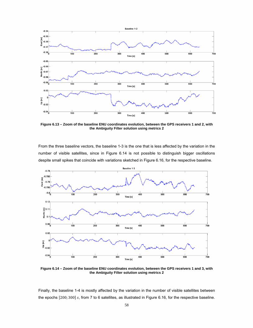
58
Figure 6.13 – Zoom of the baseline ENU coordinates evolution, between the GPS receivers 1 and 2, with the Ambiguity Filter solution using metrics 2
From the three baseline vectors, the baseline 1-3 is the one that is less affected by the variation in the
number of visible satellites, since in Figure 6.14 is not possible to distinguish bigger oscillations
despite small spikes that coincide with variations sketched in Figure 6.16, for the respective baseline.
Figure 6.14 – Zoom of the baseline ENU coordinates evolution, between the GPS receivers 1 and 3, with the Ambiguity Filter solution using metrics 2
Finally, the baseline 1-4 is mostly affected by the variation in the number of visible satellites between
the epochs 200; 300 , from 7 to 6 satellites, as illustrated in Figure 6.16, for the respective baseline.

59
This centimeter-level oscillation is verified in an instantaneous increment of the East component and a
decrease of the Up component.
Figure 6.15 – Zoom of the baseline ENU coordinates evolution, between the GPS receivers 1 and 4, with the Ambiguity Filter solution using metrics 2
Figure 6.16 – Number of visible satellites for the three baseline vectors

60
These results prove that, even in noisier environments, the technique used to avoid the lost of the
correct integer ambiguity set solution, by resetting the Ambiguity Filter, is a big addition to the
algorithm improving the results presented in [8], keeping a precise and accurate solution for the
baseline vectors.
Comparison between Ambiguity Filter, LAMBDA Method, Float Solution and Smoothed
Float Solution
For the comparison between the Ambiguity Filter and the remaining techniques, the baseline vectors’
ENU coordinates, obtained with different methods, are presented in Figures 6.17, 6.18 and 6.19, for
the respective baseline.
Figure 6.17 – Baseline ENU coordinates evolution, between the GPS receivers 1 and 2, using different techniques to solve the integer ambiguity problem

61
Figure 6.18 – Baseline ENU coordinates evolution, between the GPS receivers 1 and 3, using different techniques to solve the integer ambiguity problem
Figure 6.19 – Baseline ENU coordinates evolution, between the GPS receivers 1 and 4, using different techniques to solve the integer ambiguity problem
For the three baselines the results are analogous to the ones presented for the same comparison for
the single baseline case. In fact, due to higher disturbances present in this scenario, there is
degradation in the precision level, which may be verified by comparing Tables 6.2 and 6.4. By
analyzing the Up coordinates’ performance, in Table 6.4, for all techniques it is possible to
demonstrate that in this case the precision of the solution obtained by using the Ambiguity Filter is
close to 1.3 , which is worst when compared with an accuracy of 7 for the single baseline case.
However this loss of precision is small when compared with the precision of the remaining solutions

62
that have levels in the order of several meters. This fact is illustrated in above Figures, where the
Ambiguity Filter solution is almost undisturbed when compared with the remaining ones.
Table 6.4 – Performance of the baseline ENU coordinates in the multiple baseline static trial using different techniques to solve the integer ambiguity problem
Ambiguity
Filter
LAMBDA
method
Float
Solution
Smoothed Float
Solution
Baseline
1-2
(m) 0.368 0.306 0.262 0.202
(m) 0.005 4.855 4.820 3.861
(m) -0.675 0.999 1.017 1.199
(m) 0.005 4.232 4.176 3.489
(m) 0.005 0.964 1.096 1.131
(m) 0.015 8.034 7.991 6.217
Baseline
1-3
(m) 0.793 0.687 0.677 0.645
(m) 0.003 3.201 3.183 2.373
(m) 0.103 0.328 0.327 0.326
(m) 0.003 3.422 3.372 2.608
(m) 0.009 0.487 0.544 0.550
(m) 0.010 6.727 6.662 5.003
Baseline
1-4
(m) 1.166 1.353 1.328 1.355
(m) 0.006 4.005 3.976 3.013
(m) 0.597 0.891 0.895 0.893
(m) 0.003 3.508 3.413 2.455
(m) 0.036 2.189 2.241 2.152
(m) 0.013 6.638 6.579 4.936
From these results, along with the ones presented for the single baseline trial, it is proved that from
the presented techniques only the Ambiguity Filter allow solutions with good precision to estimate the
platform’s attitude correctly
Attitude Determination
Using the baseline vectors obtained with the Ambiguity Filter as measurements, after the algorithm’s
stabilization, the attitude angles were obtained by employing both the rotation matrix technique and
the quaternion based EKF. In Figure 6.20 both solutions are presented. The blue line illustrates the
evolution of the Euler angles estimated by the rotation matrix LS. The red line depicts the evolution of
the Euler angles obtained by the quaternion based EKF. Since this is a recursive algorithm, it takes a
few seconds to stabilize in the correct values, which corresponds to the transitory in the EKF’s
solution.

63
In Figure 6.21 is presented a zoom of the attitude angles’ evolution, where it is possible to see that
both solutions are similar. However, the solution obtained through time by the EKF is smoother than
the one obtained directly from the rotation matrix, which is emphasized by the numerical performance
results depicted in Table 6.5. These results are expected, due to the recursive nature of the EKF.
Figure 6.20 – Comparison between the attitude angles obtained with the rotation matrix technique and with the quaternion based EKF
Figure 6.21 – Zoom of the comparison between the attitude angles obtained with the rotation matrix technique and with the quaternion based EKF

64
Table 6.5 – Performance of the attitude angles estimation, using the rotation matrix technique and the quaternion based EKF
Rotation Matrix Quaternion Based EKF
Pitch Angle (°) 0.666 1.007
(°) 1.001 0.708
Roll Angle (°) 0.277 0.147
(°) 0.709 0.751
Heading Angle (°) 115.193 117.008
(°) 0.261 0.212
As aforementioned, only the baseline vectors are used as measurements. Thus, the angular velocities
are estimated in the EKF, and its evolution is depicted in Figure 6.22. As expected, the presented
results for the angular velocities converge to zero, since the platform has no motion. This fact
demonstrates that the dynamic system is correctly design, since the angular velocities are correctly
estimated by using only the baseline vectors’ measurements.
Figure 6.22 – Angular velocities estimated with the quaternion base EKF during the static trial
Since there is not information about the real value of the attitude angles, the innovation process may
be used to evaluate the EKF performance. The evolution of the innovation for each baseline is
depicted in Figures 6.23, 6.24 and 6.25, and the respective performance is resumed in Table 6.6. The
results present that the mean value of the innovation process is close to zero and that its precision is
close to the millimeter-level.

65
Figure 6.23 – Innovation process between the measured baseline 1-2 and the one obtained with the estimated quaternion
Figure 6.24 – Innovation process between the measured baseline 1-3 and the one obtained with the estimated quaternion

66
Figure 6.25 – Innovation process between the measured baseline 1-4 and the one obtained with the estimated quaternion
Table 6.6 – Performance of the innovation process for each baseline, during the static trial
Baseline 1-2 Baseline 1-3 Baseline 1-4
. ( ) 0.020 0.011 0.004
. ( ) 0.003 0.006 0.008
. ( ) 0.033 0.003 0.032
. ( ) 0.004 0.004 0.005
. ( ) 0.009 0.009 0.017
. ( ) 0.008 0.010 0.008
6.3 Dynamic Trial Results
At this point it is clear that only the baseline solution obtained with the best integer ambiguities,
provided by the Ambiguity Filter, allow high levels of confidence in attitude determination. As
aforementioned, the same platform used for the multiple baseline static trial was in motion with the
trajectory previously depicted by Figure 5.9. The corresponding Euler angles are depicted in Figure
6.26. The attitude algorithms’ solution is only available after the correct integer ambiguity is known,
that is, when the stabilization of the Ambiguity Filter is achieved. Around the epoch 150 the
platform starts moving, which is characterized by the heading variation and the increase in the
disturbances present in both pitch and roll angles. As for the static case, in the first epochs the EKF’s
solution is characterized by a transitory preceding the convergence of the state variables around the
correct solution.

67
Figure 6.26 – Comparison between the attitude angles obtained with the rotation matrix technique and with the quaternion based EKF, for the dynamic trial
By analyzing Figure 6.26 along with the zoom of pitch and roll angles in Figure 6.27, one may verify
that at the beginning, around epoch 150 , of the trajectory the roll angle estimated by the EKF is
highly disturbed when compared with the solution obtained by the rotation matrix. This fact is
emphasized by the term of the angular velocity after the platform start moving in Figure 6.30, which
is not exact since the maneuvers made during the trial were with small accelerations. This may be
explained by the decrease of precision in the Up coordinate after the platform started moving, which is
represented in Figure 6.28. This could be improved by using an accelerometer output as
measurement of the EKF and hence to better estimate the angular velocities.
Figure 6.27 – Zoom of pitch and roll angles obtained with the rotation matrix technique and with the quaternion based EKF, for the dynamic trial

68
Figure 6.28 – Up coordinate evolution of the three baselines after stabilization
During this trial a positive roll angle was imposed to the car used as platform by climbing the side walk
only with the left side wheels, between epochs ∈ 235; 245 and when the vehicle’s heading was
30°. This test’s result is depicted in Figure 6.29, where it is possible to see that the roll angle
evolution is approximately 5° for both techniques at epoch 240 , which corresponds to the positive
rotation about the -axis applied to the vehicle.
Figure 6.29 – Zoom of heading and roll angles, during a positive rotation about the axis (positive roll angle), obtained with the rotation matrix technique and with the quaternion based EKF, for the dynamic
trial

69
Figure 6.30 – Evolution of the angular velocities estimated by the EKF during the dynamic trial
As for the static case, the innovation process is used to evaluate the performance of the EKF. But in
the dynamic trial case, the movement increased the disturbances present in the measurements as
already illustrated in Figure 6.28 for the baselines’ Up coordinates. This fact is illustrated too in the
evolution of the innovation process, where the initial instant 1 corresponds to the epoch when the
Ambiguity Filter achieved the optimal solution, that is 57 . So the vehicle starts moving when the
innovation process is close to 100 in Figures 6.31, 6.32 and 6.33, for the respective baselines.
As expected the innovation of each baseline coordinate is zero mean but in contrast with the static
case higher residual levels are indentified, which are recursively compensated by the Kalman gain.
Despite the good results presented by the EKF in this dynamic trial, this solution could not be
applicable with highly disturbed measurements that lead to residual levels outside the boundaries of
the stability region. The performance of the EKF is resumed in Table 6.7, where it is possible to
confirm that the average innovation for each baseline is around zero and that the standard deviation
varies from several millimeters to several centimeters, representing a slight degradation as expected
when comparing with the results for the static trial in Table 6.6.

70
Figure 6.31 – Evolution of the innovation process between the measured baseline1-2 and the one obtained by the estimated quaternion, during the dynamic trial
Figure 6.32 – Evolution of the innovation process between the measured baseline1-3 and the one obtained by the estimated quaternion, during the dynamic trial

71
Figure 6.33 – Evolution of the innovation process between the measured baseline1-4 and the one obtained by the estimated quaternion, during the dynamic trial
Table 6.7 – Performance of the innovation process for each baseline, during the dynamic trial
Baseline 1-2 Baseline 1-3 Baseline 1-4
. ( ) 0.015 0.007 0.021
. ( ) 0.066 0.070 0.107
. ( ) 0.007 0.002 0.006
. ( ) 0.076 0.069 0.125
. ( ) 0.011 0.011 0.015
. ( ) 0.027 0.024 0.033
Despite the degradation of the disturbances in a dynamic trial, the EKF performance is good and the
results validate this technique. The direct use of the rotation matrix allow similar results, however lacks
in the stability that is allowed by a recursive algorithm (i.e. inside the stability region of the EKF) and in
the presence of singularities. Better results could be achieved by GNSS/INS coupling techniques.

72

73
7 CONCLUSIONS
The implementation of an attitude determination algorithm, using multiple L1 GPS receivers and RTK
techniques, was the main objective of this thesis. Based on the results presented in the previous
chapter, it is possible to conclude that this objective was successfully achieved.
The static trial results showed that resorting to both the algorithm using the rotation matrix and the
quaternion based EKF, it was possible to estimate the Euler angles with precisions smaller than 1°
(1 ). However, the quaternion based EKF showed slight improvements regarding the estimation of
both pitch and heading angles with an increased precision in the order of approximated 0.3° and 0.05°,
respectively, which is understandable since it is a recursive estimation algorithm. The good
performance of the EKF is visible in the innovation results, which have millimeter level errors (1 )
Despite the disturbances augmentation, the dynamic results are representative of the successfully
implementation of the attitude determination algorithms, capable of detecting attitude variations along
the path made by the test platform. This fact was visible in the detection of a positive roll angle (of
approximately 6°), imposed by climbing a sidewalk with the test vehicle. The increase in the level of
disturbances is visible in the attitude angles that are function of the Up coordinate (which is more
sensible to noise), that is, pitch and roll angles. For the EKF the roll angle is more affected by this
phenomenon, since the highly disturbed Up coordinate led to a highly disturbed angular velocity about
the axis. However these disturbances do not affect the correct determination of the Euler angles,
which is proved by the performance of the EKF innovation. Despite the disturbances’ augmentation,
the innovation has errors in the order of the centimeter (1 ).
The static trials showed that the use of the LAMBDA method along with the Ambiguity Filter allows
higher confidence in the determination of the correct integer ambiguity, and hence a millimeter level
precision in the determination of the baseline vector. In contrast, the baseline solution of the remaining
methods (stand alone LAMBDA method, Float Solution and Smoothed Float Solution) was obtained
with a meter level precision.
The static results, for single and multiple baselines showed that the proposed improvements within the
Ambiguity Filter offer an increase of this algorithm’s accuracy. The metric 2, using the baseline length
and the Up coordinate in an initial state, offered more confidence in determining the correct integer
ambiguity than the metric 1, using the baseline length along with the carrier phase residuals. The
introduction of a technique able to keep the correct integer ambiguity solution despite the variation in
the satellites’ constellation is another improvement within the Ambiguity Filter. This technique avoids
resetting the algorithm and hence the restart of the search process for the integer ambiguity
determination, which permits the loss of precision in the baseline solution. The results showed that,
despite some oscillations due to variations in the satellites’ constellation, it is possible to obtain a

74
millimeter level precision, and hence a precision smaller than 1° (1 ) in the determination of the Euler
angles. In the low multipath scenario of the single baseline static trial, the precision of both heading
and pitch angles was approximately 0.01° and 0.03°, respectively.
Despite the good results, there are topics that could be improved. Thus some topics regarding future
work are presented:
The research for better metrics and stabilization procedures for the Ambiguity Filter. Despite of
the great precision, the technique responsible for avoiding the loss of solution could be
improved and tested for longer periods for a more robust validation;
The research and test of different estimation techniques and different dynamic systems for
comparison with the ones implemented in this thesis, in order to improve the presented
results;
The use of techniques like the Constrained Kalman Filter, that allow a coupled estimation of all
baselines, making use of the dynamic information given by the GPS receivers’ Doppler effect
and the satellites’ velocity;
In order to avoid the verified disturbances in the Up coordinate, that were translated in a
precision degradation on the estimated angular velocity about the axis, and consequently in
roll angle, the integration of the developed technique with INS sensors (accelerometers in
order to improve the estimation of the angular velocities) could lead to great improvements;
Real time implementation and test in more aggressive environments of the proposed
algorithms;
Even though is not present in this thesis, research regarding the development of an attitude
test platform has already been started. A test platform that allows the imposition of different
attitude angles could be a great advantage in algorithms validation.

75
REFERENCES
[1] E. D. Kaplan and C. J. Hegarty, Understanding GPS: principles and applications, 2nd ed. Artech House Publishers, 2006.
[2] ESA “Galileo fact sheet,” 2011.
[3] P. Misra and P. Enge, Global Positioning System : Signals , Measurements , and Performance, 2nd ed. Ganga-Jamuna Press, 2006.
[4] D. Kim and R. B. Langley, “GPS Ambiguity Resolution and Validation : Methodologies , Trends and Issues,” International Symposium on GPS/GNSS, Seoul, Korea, 2000.
[5] P. Teunissen, “Least-Squares Estimation of the Integer GPS Ambiguities,” Delft Geodetic Computing Centre LGR series, no 6., 1993.
[6] G. Strang and K. Borre, Linear algebra, geodesy, and GPS. Wellesley Cambridge Pr, 1997.
[7] G. Giorgi, P. J. G. Teunissen, and P. J. Buist, “A Search and Shrink Approach for the Baseline Constrained LAMBDA Method : Experimental Results,” International Symposium GPS/GNSS, pp. 797-806, Tokyo, 2008.
[8] J. Reis, “Real-time GPS Heading Determination,” MSc Thesis, Instituto Superior Técnico, Technical University of Lisbon, November 2009.
[9] J. Reis, J. Sanguino, and A. Rodrigues, “Impact of Satellite Coverage in Single-Frequency Precise Heading Determination,” in Position Location and Navigation Symposium (PLANS), 2010 IEEE/ION, Indian Wells, USA, 3-6 May 2010, pp. 592-597.
[10] J. Reis, J. Sanguino, and A. Rodrigues, “Baseline Influence on Single-Frequency GPS Precise Heading Estimation,” in Wireless Personal Communications Journal, Springer, Netherlands, 2012.
[11] J. Reis, J. Sanguino, A. Rodrigues, “Influence of Baseline Length in Single-Frequency Real-Time Vehicle Heading Estimation,” in The 13th International Symposium on Wireless Personal Multimedia Communications (WPMC), Recife, Brazil, 11-14 October 2010.
[12] P. Batista, C. Silvestre, and P. Oliveira, “Partial Attitude and Rate Gyro Bias Estimation: Observability Analysis, Filter Design, and Performance Evaluation,” International Journal of Control, vol. 84, no. 5, pp. 895-903, May 2011.
[13] S. Brás, R. Cunha, J. F. Vasconcelos, C. Silvestre, and P. Oliveira, “A Nonlinear Attitude Observer Based on Active Vision and Inertial Measurements,” IEEE Transactions on Robotics, vol. 27, no. 4, pp. 664-677, 2011.
[14] S. Brás, C. Silvestre, P. Oliveira, J. F. Vasconcelos, and R. Cunha, “An Experimentally Validated Attitude Observer Based on Range and Inertial,” IFAC World Congress, Italy, September 2011.
[15] E. Edwan, S. Knedlik, J. Zhou, and O. Loffeld, “A Constrained GPS / INS Integration Based on Rotation Angle for Attitude Update and Dynamic Models for Position Update,” International Technical Meeting of The Institute of Navigation pp. 736-743, Anaheim, CA,2009.

76
[16] J. F. M. Lorga , P. F. Silva, J. S. Silva, and A. Fernández, “Attitude Determination Using a Multi-antenna GNSS Receiver Tightly Integrated with a MEMS IMU,” 20th International Technical Meeting of the Satellite Division of the Institute of Navigation, September 2007. September, pp. 25-28, 2007.
[17] G. Giorgi, P. J. Buist, S. Verhagen, P.J.G. Teunissen, “GNSS-Based Attitude Determination,” InsideGNSS, July/August 2011.
[18] J. Tsui, “Fundamentals of Global Positioning System Receivers, A Software Approach. 2nd edition,” John Wiley & Sons, New York, vol. 2, no. 4, 2005.
[19] Colonel B. Gruber “Status and Modernization of the US Global Global Positioning System,” Satellite Navigation Summit, Munich, Germany, March 2012.
[20] GPS official website, www.gps.gov, visited on April 2012.
[21] Global Positioning System Wing Systems Engineering & Integration, “Interface Specification IS-GPS-200 (Revision E),” El Segundo, CA, June, 2010.
[22] R. A. Serway and J. W. Jewett, Physics for scientists and engineers, vol. 1. Brooks/Cole Pub Co, 2009.
[23] B. Hoffmann-Wellenhof, H. Lichtenegger, and J. Collins, “GPS: Theory and practice,” Springer-Verlag, New York, pp. 2-5, 1994.
[24] J. Sanguino, Lecture Notes on: "Navigation System,” 2010.
[25] R. E. Kalman, “A New Approach to Linear Filtering and Prediction Problems,” Transactions of the ASME - Journal of Basic Engineering, vol. 82, no. Series D, pp. 35-45, 1960.
[26] G. Welch and G. Bishop, “An Introduction to the Kalman Filter,”, 2006.
[27] D. Simon, Optimal state estimation: Kalman, H [infinity] and nonlinear approaches. John Wiley and Sons, 2006.
[28] F. V. Graas and M. Braasch, “GPS Interferometric Attitude and Heading Determination: Initial Flight Test Results,” The Institute of Navigation, vol. IV, pp. 359-378, 1991.
[29] P. J. D. Jonge, C. C. J. M. Tiberius, P. J. G. Teunissen, and G. C. Centre, “Computational Aspects of the LAMBDA Method for GPS Ambiguity Resolution,” Proceedings of ION GPS-96, 9th International Technical Meeting of the Satellite Division of the Institute of Navigation, Kansas City, Missouri, Sept.17-20, pp 935-944.
[30] J. B. Kuipers, Quaternions and rotation sequences, vol. 1. Princeton university press Princeton, NJ, 1999.
[31] J. B. Schleppe, “Development of a Real-Time Attitude System Using a Quaternion Parameterization and Non-Dedicated GPS Receivers,” Master Thesis, Department of Geomatics Engineering, University of Calgary, 1996.
[32] Y. T. Chiang, L. S. Wang, F. R. Chang, and H. M. Peng, “Constrained Filtering Method for Attitude Determination using GPS and Gyro,” IEE Proceedings - Radar, Sonar and Navigation, vol. 149, no. 5, p. 258, 2002.
[33] Y. Bar-Shalom, X. Li, and T. Kirubarajan, Estimation with applications to tracking and navigation, vol. 9. 2001.

77
[34] F. Nunes, Lecture Notes on: “Sistemas de Controlo de Tráfego,” 2010.
[35] Wilson J.Rugh, Linear system theory, Second. 1996.
[36] Magellan, "A12, B12 & AC12 Reference Manual," 2005.
[37] U-Blox, “u-blox 6 Receiver Description,” 2010.
[38] Novatel, "531 Rev. 2 and A032 Data Sheets", 1999.
[39] U-Blox, “ANN Active GPS Antenna,” 2003.
[40] KML Documentation, https://developers.google.com/kml/documentation/, visited on April 2012.
Top Related