
Yoan David Ribeiro -...
118
Universidade do Minho Escola de Engenharia Departamento de Informática Yoan David Ribeiro Validation of IEC 61131-3 Programmable Logical Controllers in KeYmaera October 2015
Transcript of Yoan David Ribeiro -...

Universidade do MinhoEscola de EngenhariaDepartamento de Informática
Yoan David Ribeiro
Validation of IEC 61131-3Programmable Logical Controllers in KeYmaera
October 2015

Universidade do MinhoEscola de EngenhariaDepartamento de Informática
Yoan David Ribeiro
Validation of IEC 61131-3Programmable Logical Controllers in KeYmaera
Master dissertationMaster Degree in Computing Engineering
Dissertation supervised byLuís Soares BarbosaAlexandre Madeira
October 2015


AC K N OW L E D G E M E N T S
This page is always a little awkward and some might think embarrassing but let me tell you:
There is no shame in being grateful for someone or something, on the contrary, gratitude is what
makes us happy, it is what make us bond with one another, it enriches our lives. I could go on with
the benefits of gratitude but I would not be thanking anyone that way.
So, this dissertation would not be possible without the careful watch of my supervisors Prof. Luís
Barbosa and Alexandre Madeira. I have learnt greatly with them and I am grateful for the opportunity
that they gave me, their patience and positive input, many thanks. I have to thank Prof. José Nuno
Oliveira for the inspiration that he continuously gives me and so many other students, to do our best
and pursue our passions. I am also grateful to Prof. António Martins and Renato for their opinions,
positive feedback and being always ready to help.
Of course I am grateful for my friends and their will to help me whenever they can, specially to the
MFES Way crew, with no particular order: Ana, Damien, Paulo, Lobo, Luís, Vitor, Fábio Fernandes,
Catarina, Fábio Esteves, João, Telma, Nuno, Miguel, Rogério thank you so much for helping me and
becoming a better version of myself!
And last but definitely not least, my family. Without them I would not be where I am; they are the
foundation of the person I am today. Dad, Nela, Sara, Diego, Patrícia, Ruben and so on. I am lucky to
call you my Family, thank you for everything, I am forever grateful for what you have done for me.
Thank you very much to everyone that in one way or another helped me in this journey so far and
do not forget there is no shame in being grateful because, as Cicero said:
"Gratitude is not only the greatest virtue, but the parent of all the others"
a


AC K N OW L E D G E M E N T S
This work is financed by the ERDF - European Regional Development Fund through the COM-
PETE Programme (operational programme for competitiveness) and by National Funds through the
FCT - Fundação para a Ciência e a Tecnologia (Portuguese Foundation for Science and Technology)
within project FCOMP-01-0124- FEDER-028923
c


A B S T R AC T
PLCs (Programmable Logical Controllers) are embedded computers built specifically for the indus-
trial environment, and used for the automation of industrial processes. These systems are typically
developed resorting to programming languages defined in the IEC 61131-3 standard, which includes
two textual and three graphical programming languages. IEC 61131-3 has become widely established
in recent years as the programming standard for industrial automation. Actually, a wide range of small
to large PLC manufacturers offer programming systems that are based on it. Methods to formally anal-
yse PLCs developed in this framework are needed, namely to provide timing guarantees as well as to
quantify the dependability parameters of the resulting applications. In this dissertation we propose to
tackle these issues resorting to the KEYMAERA verification tool and its associated dynamic logic for
hybrid systems. KEYMAERA is a verification tool for hybrid systems supporting differential dynamic
logic (dL), which combines deductive, real algebraic, and computer algebraic prover technologies. dL
is a suitable logic to deal with hybrid systems, that combines first-order dynamic logic, whose atomic
programs are variables assignments (to represent discrete evolutions), with ordinary differential equa-
tions (to represent continuous evolutions). The dissertation is devoted to the design and development
of a practical validation framework for IEC 61131-3 PLCs based on KEYMAERA. This involves
the development of a translator from the controller program to the discrete (cyber) component of a
KEYMAERA model and the specification of contextual conditions (e.g. measured by sensors in real
scenarios) as the continuous (physical) component of the model. The whole research guided guided
by some case studies.
e


R E S U M O
PLC (Programmable Logical Controllers) são computadores embebidos construídos para o ambiente
industrial, e usados em automação de processos industriais. Estes sistemas são tipicamente progra-
mados recorrendo às linguagens de programação definidas na norma IEC 61131-3, que inclui duas
linguagens de programação textuais e três gráficas. Actualmente, uma grande variedade de pequenos
e grandes construtores de PLC oferecem sistemas de programação baseados nessas linguagens. Méto-
dos para uma análise formal de PLCs construídos nessa framework são necessários, nomeadamente
para providenciar garantias de tempo assim como a quantificação de parâmetros de confiança das
aplicações resultantes. Nesta dissertação abordam-se estes problemas recorrendo à ferramenta de ver-
ificação KEYMAERA e à sua lógica dinâmica associada para os sistemas híbridos. KEYMAERA é uma
ferramenta de verificação para sistemas híbridos que suporta lógica dinâmica diferencial (dL), combi-
nando tecnologias prover deductive, real algebraic e computer algebraic. dL é uma lógica dinâmica
de primeira ordem para programas híbridos. dL é uma lógica adequada ao tratamento de sistemas
híbridos, que combina lógica dinâmica de primeira ordem, cujos programas atómicos consistem em
valorações de variáveis (para modelar evoluções discretas) com equações diferenciais ordinárias (para
modelar evoluções contínuas). Esta dissertação foca-se na concepção de um framework de validação
prática para PLCs IEC 61131-3 baseada em KEYMAERA. Tal envolve a construção de um tradutor
para o programa do controlador para um componente discreto (cíber) de um modelo KEYMAERA e
a especificação de condições de contexto (e.g. em casos reais, medidas por sensores) como a compo-
nente contínua (física) do modelo. A investigação foi guiada por alguns casos de estudo.
g


C O N T E N T S
Contents iii
1 I N T RO D U C T I O N 3
1.1 Motivation 3
1.2 Context 4
1.3 Contribution 5
1.4 Roadmap 5
2 B AC K G RO U N D A N D S TAT E O F T H E A RT 7
2.1 Programmable Logic Controller 7
2.1.1 IEC 61131-3 7
2.1.2 Tools to build programs for PLCs 13
2.1.3 Beremiz 13
2.2 Cyber-Physical Systems 14
2.2.1 Hybrid Automata 14
2.2.2 Specification languages for cyber-physical system 15
2.2.3 Model Checkers for Hybrid Automata 16
2.2.4 KEYMAERA 17
2.3 Formalisation of PLC programs 18
3 S F C T O K E Y M A E R A : T H E A P P RO AC H 21
3.1 Sequential Function Charts plus Differential Equations 21
3.1.1 SFC Syntax 22
3.1.2 SFC semantics 23
3.1.3 Conditional ordinary differential equations 24
3.2 Beremiz SFC to Haskell SFC 25
3.2.1 SFCHXT 25
3.3 SFC annotation 29
3.4 From SFC annotated to Hybrid Automata 31
3.4.1 From SFC to Hybrid Automaton 31
3.4.2 From SFCs and CODES to Hybrid Automaton 33
3.5 Hybrid Automata to KeYmaera 34
4 C A S E S T U DY: T H E WAT E R H E AT I N G TA N K 36
4.1 Description of the problem 36
4.2 The SFC program and the generated model 37
4.2.1 Program and annotations 37
iii
Contents
4.2.2 Model obtained 40
4.3 Verifying safety properties 44
5 C A S E S T U DY: T H E P H P L A N T 48
5.1 Description of the problem 48
5.2 The SFC program and the generated model 49
5.2.1 Program and annotations 49
5.2.2 Model obtained 51
5.3 Verifying Safety property 58
6 C O N C L U S I O N A N D F U T U R E W O R K 59
6.1 Achievements 59
6.2 Future work 59
A AU X I L A RY W O R K : S T T O K E Y M A E R A 67
B T O O L S T RU C T U R E : S F C H X T 69
C T O O L S T RU C T U R E : S F C 70
D T O O L S T RU C T U R E : H Y B R I D AU T O M AT O N 71
E C A S E S T U DY: WAT E R H E AT I N G TA N K X M L 72
F C A S E S T U DY: P H P L A N T X M L 81
iv
L I S T O F F I G U R E S
Figure 1 Roadmap of the dissertation. 6
Figure 2 An hybrid automata representing a thermostat. 15
Figure 3 Transformation of SFC XML to KEYMAERA. 21
Figure 4 Transformation SFC to Hybrid Automaton. 33
Figure 5 Adaptation of annotated step to Hybrid automaton. 33
Figure 6 SFC program of the water heating tank problem. 38
Figure 7 Water heating tank program with annotation in Beremiz IDE. 39
Figure 8 The resulting message given by the tool after processing the PLC program. 39
Figure 9 KEYMAERA window with the proof success message. 45
Figure 10 KEYMAERA window with the proof success message with the temperature
condition. 46
Figure 11 KEYMAERA window on an unsuccessful attempt to prove y = 0. 46
Figure 12 SFC program representing the pH plant problem. 50
Figure 13 pH plant program with annotation in Beremiz IDE. 51
Figure 14 KEYMAERA window proving the safety property of the pH plant. 58
v


L I S T O F TA B L E S
Table 1 ST code and explanation. 9
Table 2 SFC graphical code and explanation. 12
Table 3 dL operators and their informal meaning. 18
Table 4 ST code to KEYMAERA hybrid program 68
vii

L I S T O F L I S T I N G S
A.1 . . . . . . . . . . . . . . . . . . . . . . . . . . . . . . . . . . . . . . . . . . . . . 67
A.2 . . . . . . . . . . . . . . . . . . . . . . . . . . . . . . . . . . . . . . . . . . . . . 67
A.3 . . . . . . . . . . . . . . . . . . . . . . . . . . . . . . . . . . . . . . . . . . . . . 67
A.4 . . . . . . . . . . . . . . . . . . . . . . . . . . . . . . . . . . . . . . . . . . . . . 68
A.5 . . . . . . . . . . . . . . . . . . . . . . . . . . . . . . . . . . . . . . . . . . . . . 68
A.6 . . . . . . . . . . . . . . . . . . . . . . . . . . . . . . . . . . . . . . . . . . . . . 68
A.7 . . . . . . . . . . . . . . . . . . . . . . . . . . . . . . . . . . . . . . . . . . . . . 68
A.8 . . . . . . . . . . . . . . . . . . . . . . . . . . . . . . . . . . . . . . . . . . . . . 68
A.9 . . . . . . . . . . . . . . . . . . . . . . . . . . . . . . . . . . . . . . . . . . . . . 68
ix

1
I N T RO D U C T I O N
The world, nowadays, relies on software for everything for instance in cars, aircrafts, medical tools
and other domains of application. From this extensive use of software a question arises: Can we
trust the software running on those systems? A honest answer to this question is: it depends. Some
will be safe, and others will not and that is because not every entity responsible for building software
uses formal methods. Formal methods are more crucial than ever because we, human beings need
to be sure that the software that we use in our every day life is reliable and safe to use. This is only
possible if mathematical based techniques are used to specify and verify software. This dissertation
aims to apply formal methods to validate a subset of the IEC 61131-3 standard, for programmable
logic controllers, programming languages using KEYMAERA which is a theorem prover suitable for
some classes of cyber-physical systems.
1.1 M OT I VAT I O N
Programmable Logic Controllers (PLCs) are embedded computers used for industrial automation and
programmed according to the standard IEC 61131-3 (John and Tiegelkamp, 2010). As any other
system, PLCs have to, somehow, be verified and tested.
Simulation focuses mainly in the behavioural part of a program/system and usually provides a visual
representation of the system which makes it more tangible. Consequently, this technique constitutes
the usual method used to verify if the PLC program follows its behaviour. Note however this technique
cannot prove, for instance, that a given behaviour will always or never occur, leading to a incomplete
verification.
Besides simulation, model-checking is also widely used technique in formal methods. It focuses
on proving that a set of proprieties meets the specification given by a model. Although a powerful
method to find errors in a model, model-checking only proves correctness to a finite-state system
which implies that it is often not sufficient to prove that the model is without fault.
The technique used in this dissertation is verification through a theorem prover. When given a
model, which represents the system or more specifically the PLC program, this method goes through
all the possibilities to verify if the given model follows the set of proprieties.
3

Chapter 1. I N T R O D U C T I O N
Furthermore, it is well known that PLCs interact with the world through sensors and evaluate the
information provided by the sensor to discretely change their behaviour if necessary. Therefore, these
systems can be classified as cyber-physical systems.
Cyber-physical systems are systems which contain computational elements that interact and control
physical entities. These systems are also known as embedded systems with a emphasis in the intense
link between the computational and physical elements. Consequently, they exhibit both continuous
dynamics and a discrete dynamics. To prove specific properties about such systems, the theorem
prover KEYMAERA uses differential dynamic logic (dL) (Platzer, 2010), and combines a deductive
prover and computer algebraic solvers technologies.
After recognizing that programmable logical controllers can be seen as cyber-physical system, the
next step is to set up a framework for their validation. The step will consist of transforming the
programs which are ran by PLCs to KEYMAERA models and resort to that tool to prove them.
Summing up, this dissertation aims at showing how to verify PLC programmed according to the
standard IEC 61131-3 using KEYMAERA.
1.2 C O N T E X T
The Nasoni project, which gives the context to this dissertation, proposes to study software composi-
tion in the domain of the coordination paradigm which integrate different and often loosely coupled
software entities, as is the case of PLCs.
The focus of this dissertation is to translate the languages used to build programmable logic con-
trollers into KEYMAERA formulas. The strategy to achieve such a goal resorts to a set of case studies
to better understand the differences and, more importantly, the similarities between the languages of
the IEC-61131-3 and KEYMAERA hybrid programs, and then to design a program able to translate
most of the norm to KEYMAERA.
The IEC-61131-3 determines how PLCs are built, and not only the language in which the controllers
are programmed, but also, how the PLC programs should be designed. The norm defines five different
languages to build PLC programs:
• Instruction List;
• Structured Text;
• Function Block Diagram;
• Ladder Diagram;
• Sequential Function Charts.
The first two are textual and the remaining three are graphical (although sequential function charts has
also a textual representation).
4

1.3. Contribution
After understanding how PLC programs are built within the standard, it is necessary to design
their translation to a KEYMAERA hybrid program. Certainly, the translation process has various
steps, depending on the target language. In particular, this dissertation will focus mainly on the
graphical language sequential function charts because of its resemblance to automata, which eases
the translation process.
1.3 C O N T R I B U T I O N
The main contribution of this dissertation is to provide a basic tool to verify PLC programs by gener-
ating a KEYMAERA model based on the program. The method underlying such transformation is the
formalisation of the sequential function chart with conditional ordinary differential equations, CODE
for shorts, discussed in (Nellen and Ábrahám, 2012).
To achieve such a goal, an annotation language was designed to enrich the SFC language of
Beremiz, which is the IDE in which PLC programs are developed.
With the tool, two case studies were designed to test and evaluate its potential.
1.4 RO A D M A P
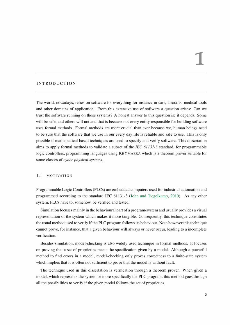
After exposing the motivation, context and contribution of this dissertation, the remaining chapters
are arranged as follows, (see Figure 1):
C H A P T E R 2 covers the background for this dissertation, namely, the languages for the PLC pro-
grams, cyber-physical systems and respective models as well as the KEYMAERA theorem
prover. Furthermore, it provides a solid overview of the tools used to build PLC programs
emphasising the Beremiz IDE since it was the one used throughout this dissertation. This in-
cludes the methods used to model cyber-physical systems and the various formalisations of the
PLC programming languages.
C H A P T E R 3 is the core chapter of this dissertation. It details the overall approach and tool to trans-
late the SFC language annotated to KEYMAERA.
C H A P T E R 4 A N D 5 are a support chapter, describing the case studies of the water heating tank and
pH plant and how to go from the SFC code with the annotations to KEYMAERA hybrid program.
The latter is used to prove a number of safety proprieties.
C H A P T E R 6 discusses the conclusions of this dissertation.
A P P E N D I X A is an auxiliary work where it is show case the translation from structured text to
KEYMAERA.
5
Chapter 1. I N T R O D U C T I O N
A P P E N D I C E S B , C A N D D contain the Haskell data structure of the different stages of the transla-
tion to build insight on how the tool was design. Appendix E and F contain the XML file of the
case studies obtained by the Beremiz IDE.
Ch.2
Ch.3
Ap.B
Ap.C
Ap.D
Ch.4 Ch.5
Ap.E Ap.F
SFC+ to KeYmaera
Figure 1.: Roadmap of the dissertation.
6
2
BAC K G RO U N D A N D S TAT E O F T H E A RT
This chapter reviews the state of the art and background which serves as a warm up for the remaining
of the dissertation. It covers the basic concepts necessary to a full understanding of this document.
As well as the different tools and ideas which have been developed and implemented in the areas
addressed this dissertation. These are the cyber-physical systems (hybrid systems), automation, more
particularly, programmable logic controllers and formalisations of standard IEC 61131-3.
2.1 P RO G R A M M A B L E L O G I C C O N T RO L L E R
Industrial automation involves the use of multiple control systems, which are devices that administer,
direct, command or adapt the behaviour of other devices or systems. For operating equipment, namely
manufacturing processes, industrial machinery and many others often requires none or minimum hu-
man intervention, the most used control systems are the programmable logic controllers.
Programmable logic controllers (John and Tiegelkamp, 2010) are digital computer devices designed
for multiple analogue and digital inputs and output arrangements. They must be resistant to vibrations
and impacts, durable to extended temperature ranges and immune to electrical noise. The programs
which are responsible for the machine usually are stored in battery-backed-up or ROM. PLCs are an
example of hard real-time systems due to the limited time in which the output must be produced in
response to input conditions.
IEC 61131-3 (John and Tiegelkamp, 2010) is the standard used to describe the PLC programming
languages. The standard provides comprehensive concepts and guidelines for creating PLC projects.
2.1.1 IEC 61131-3
Program Organisation Unit (POU)
This component may be seen as a block which runs a set of instructions. It is the smallest independent
software unit. There are three types of POU:
• Function (FUN), units of this type behave as functions, always returning the same result, for the
same input parameters, i.e. they have no memory;
7

Chapter 2. B AC K G R O U N D A N D S TAT E O F T H E A RT
• Function block (FB), units of this kind have their own data record which saves status informa-
tion that the programmer can instantiate;
• Program (PROG), the "top" POU of a PLC program, it has the ability to access the PLC I/Os
and make them accessible to other POU.
Each of these program organisation units is divided in two main parts: The declaration part which,
as the name suggests, is where the variables are declared and, the code part, where the PLC program
is coded. The variables can be global, input, output, input/output and others and have to inhabit a
specific data type: Byte, Bool, Integer etc.
The IEC 61131-3 provides three textual languages and three graphical languages for writing appli-
cation programs (the code part of a POU). The textual languages are (John and Tiegelkamp, 2010):
• Instruction List (IL);
• Structured Text (ST);
• Sequential Functional Chart (textual version of SFC).
And the graphical languages are:
• Ladder Diagram (LD);
• Function Block Diagram (FBD);
• Sequential Function Chart (graphical version of SFC).
The instruction list is an assembly like language, which gives to the programmers the opportunity
to work at a relatively low level, meaning that there is nearly no abstraction from the PLC instruction
set architecture. IL is largely used and is frequently employed as an intermediate language to which
other textual and graphical languages are translated.
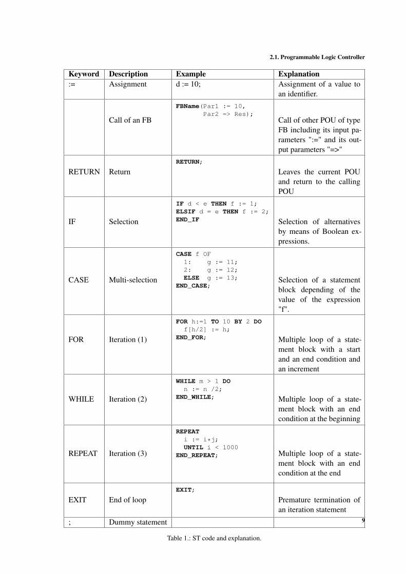
The second language, structured text, consists of a sequence of statements, just as a classic imper-
ative languages, namely, PASCAL and C. These statements consist of a combination of keywords
which control the program execution and expressions which are operators/functions and operands to
be evaluated at run time .
The Table 1 sums up the overall statements of the ST language.
8
2.1. Programmable Logic Controller
Keyword Description Example Explanation:= Assignment d := 10; Assignment of a value to
an identifier.
Call of an FB
FBName(Par1 := 10,Par2 => Res);
Call of other POU of typeFB including its input pa-rameters ":=" and its out-put parameters "=>"
RETURN ReturnRETURN;
Leaves the current POUand return to the callingPOU
IF Selection
IF d < e THEN f := 1;ELSIF d = e THEN f := 2;END_IF Selection of alternatives
by means of Boolean ex-pressions.
CASE Multi-selection
CASE f OF1: g := 11;2: g := 12;ELSE g := 13;
END_CASE;Selection of a statementblock depending of thevalue of the expression"f".
FOR Iteration (1)
FOR h:=1 TO 10 BY 2 DOf[h/2] := h;
END_FOR; Multiple loop of a state-ment block with a startand an end condition andan increment
WHILE Iteration (2)
WHILE m > 1 DOn := n /2;
END_WHILE; Multiple loop of a state-ment block with an endcondition at the beginning
REPEAT Iteration (3)
REPEATi := i*j;UNTIL i < 1000
END_REPEAT; Multiple loop of a state-ment block with an endcondition at the end
EXIT End of loopEXIT;
Premature termination ofan iteration statement
; Dummy statement
Table 1.: ST code and explanation.
9

Chapter 2. B AC K G R O U N D A N D S TAT E O F T H E A RT
The functional block diagram and the ladder diagram languages come originally from the area of
signal processing, where integer and/or floating point values are crucial.
FBD language is graphical language in which, as the name suggests, the main components are
function blocks. These represent at the left side the input gates, which are the input variables, and
output gates at the right side. Two function blocks can communicate if the output of the first is
connected to the input of the second one. This language is popular since its appearance is similar to
that of logic circuits.
The LD language is also a graphical language which was primarily designed for processing boolean
signals. The language was initially called ladder logic because the method used to document the
design and construction of relay racks, in manufacturing and process control. This logic evolved into
the programming language known today and is part of the IEC.
Finally, Sequencial Function Chart is a language defined to break down a complex program into
smaller and more manageable units, as well as to describe the control flow between those units. With
SFC, it is possible to design sequential and parallel processes (see Table 2). This graphical language
is noticeably similar to that of state machines.
Graphical object Name and explanation
ST
SB
Φ Single Sequence: Alternation of step→ transition
→ in series. ST is deactivated and SB becomes
active, as soon as Φ evaluates to TRUE
ST
*
SB1 SB2
Φ Ψ
Divergent Path: Selection of exactly one se-
quence, evaluated from left to right. The first one
which evaluates to TRUE from left to right, deacti-
vates ST and activates the corresponding step.
10

2.1. Programmable Logic Controller
ST
*2 1
SB1 SB2
Φ Ψ
Divergent path with user-defined priority: Se-
lection of exactly one sequence, evaluated by pri-
orities defined by the user. The first to evaluate to
TRUE, with the priority order defined the user, de-
activates ST and activates the corresponding step.
ST
SB1 SB2
Ψ Φ
Divergent path under user control: Selection of
exactly one sequence. Transition (Φ and Ψ) must
be mutually exclusive and the first to evaluate to
TRUE in those conditions, deactivates ST and acti-
vates the corresponding step.
SB1 SB2
SB
Ψ Φ Convergence of sequence: The divergent paths
are combined. When one of the STn is active and
the corresponding successor transition becomes
TRUE, STn deactivates and SB is initiated.
11

Chapter 2. B AC K G R O U N D A N D S TAT E O F T H E A RT
SB1 SB2
Φ
SB
Convergence of simultaneous sequences: The
path of simultaneous path are combined. When
all STn are active and the transition Φ evaluates
to TRUE then all STn are deactivated and SB is
activated.
ST
SB1 SB2
Φ Simultaneous sequences: Simultaneous activa-
tion of all connected steps. ST is deactivated when
Φ evaluates to TRUE and all subsequent steps con-
nected via Φ become active simultaneously.
ST
SM1
SB
Φ
Θ1Θ2
Sequence Loop (Branch back) Is a combination of
the already described sequences
Table 2.: SFC graphical code and explanation.
12
2.1. Programmable Logic Controller
2.1.2 Tools to build programs for PLCs
In computer programming, it makes no big difference if what is required is a program for a cloud
application or a program for controllers. Integrated Development Environment (IDE) often comes
handy and PLC programs are not too much different. For PLC development, the search of IDEs was
focused on two criteria:
1. The IDE respects the IEC 61131-3 standard;
2. The use the IDE does not rely on the existence of a PLC.
There are many IDEs which fulfil the criteria mentioned above, for instance, CODESYS (Con-
troller Development System 1), and OpenPCS Automation Suite 2. These IDEs allow programmers
to produce PLC code using the five languages of the standard and still includes a sixth one, the CFC
(Continuous Function Chart). CODESYS compiles the programs into binary code to be transferred to
a PLC. However none of these are Open Source. The one IDE which still satisfy the above criteria
and is Open Source, is Beremiz 3. Therefore, it was the chosen platform to develop PLC programs in
this dissertation.
2.1.3 Beremiz
The Open Source IDE Beremiz is a multi-platform program that allows the writing of automation
programs always in accordance with the IEC 61131-3 standard. The public availability of the software
is granted under a GNU GPLv2.1 license. The software has the following built in modules:
• PLCOpen Editor - IEC 61131-3 Program editor;
• MATIEC - Compiler of IEC 61131-3 to ANSI-C;
• CanFestival - CANOpen Framework for interface with physical I/O;
• SVGUI - Integration tool for Human-Machine Interfaces (HMIs).
The MATIEC compiler converters programs which are built using the standard languages to equiva-
lent C code, and follows four usual steps: lexical analyser, syntax parser, semantics analyser and code
generator (Tisserant et al., 2007).
1 CODESYS software: Available at: www.3s-software.com2 Open OCS Automation Suite: Available at: www.systec-electronic.com/en/products/automation-components/development-and-configuration-tools/openpcs-iec-61131-3-automation-suite
3 Beremiz website: www.beremiz.org
13

Chapter 2. B AC K G R O U N D A N D S TAT E O F T H E A RT
2.2 C Y B E R - P H Y S I C A L S Y S T E M S
Cyber-physical systems features both discrete and continuous changes. Typically, the expression
refers to systems or embedded controllers for physical systems, for instance robots, aircrafts, trains,
cars, and others, whose continuous dynamics are governed by physical principles such as fluid/thermo
dynamics or classical mechanics. These often are critical systems, since if a malfunctioning of the
system occurs, it can endanger lives.
2.2.1 Hybrid Automata
The most popular formalism behind a cyber-physical, or hybrid system is the hybrid automata (HA).
These automata exhibit on the nodes continuous behaviour, represented by differential equations,
which can be restricted by specific invariants. The edges, which may contain attributions and jump
conditions to other nodes. These additional features reflect the behaviour of the environment in each
node. Hybrid automata can be seen as a generalisation of timed automata in (Alur and Dill, 1994).
Its formal definition was proposed in (Henzinger, 1996) and the following definition is an adaptation
presented in (Nellen and Ábrahám, 2012) based in paper (Alur et al., 1995)
Definition 1 (Hybrid automata). A hybrid automaton
H = (Loc, Var, Edge, Act, Inv, Init)
consists of a tuple where
• Loc is a finite set of locations or control modes;
• Var is a finite set of real-valued variables and V a set of valuations V. A valuation v ∈ V,
v : Var → R assigns a value to each variable. A state s ∈ Loc × V pair a location and a
valuation. The set of all states is denoted by Σ;
• Edge ∈ Loc× 2V2 × Loc is a set of edges;
• Act is a function assigning a set of time-invariant activities f : R≥0 → V to each location,
which implies, ∀l∈Loc : f ∈ Act(l) → ( f + t) ∈ Act(l) where ( f + t)(t′) = f (t + t′) forall
t, t′ ∈ R≥0. These represents the f low function in a way such, that given a location it returns
the set of differential equations of the location;
• Inv : Loc→ 2V is a function assigning an invariant to each location;
• Init ⊂ Σ×V is a set of initial states.
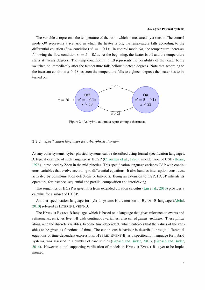
The typical example of an hybrid automata is a thermostat (Figure 2) which turns on a heater to
heat the room until the temperature is below nineteen degrees and the system turn it off the heater
whenever the latter is greater than twenty one degrees.
14
2.2. Cyber-Physical Systems
The variable x represents the temperature of the room which is measured by a sensor. The control
mode Off represents a scenario in which the heater is off, the temperature falls according to the
differential equation (flow condition) x′ = −0.1x. In control mode On, the temperature increases
following the flow condition x′ = 5− 0.1x. At the beginning, the heater is off and the temperature
starts at twenty degrees. The jump condition x < 19 represents the possibility of the heater being
switched on immediately after the temperature falls bellow nineteen degrees. Note that according to
the invariant condition x ≥ 18, as soon the temperature falls to eighteen degrees the heater has to be
turned on.
Offx′ = −0.1x
x ≥ 18x = 20
Onx′ = 5− 0.1x
x ≤ 22
x < 19
x > 21
Figure 2.: An hybrid automata representing a thermostat.
2.2.2 Specification languages for cyber-physical system
As any other systems, cyber-physical systems can be described using formal specification languages.
A typical example of such language is HCSP (Chaochen et al., 1996), an extension of CSP (Hoare,
1978), introduced by Zhou in the mid-nineties. This specification language enriches CSP with contin-
uous variables that evolve according to differential equations. It also handles interruption constructs,
activated by communication detections or timeouts. Being an extension to CSP, HCSP inherits its
operators, for instance, sequential and parallel composition and interleaving.
The semantics of HCSP is given in a from extended duration calculus (Liu et al., 2010) provides a
calculus for a subset of HCSP.
Another specification language for hybrid systems is a extension to EVENT-B language (Abrial,
2010) referred as HYBRID EVENT-B.
The HYBRID EVENT-B language, which is based on a language that gives relevance to events and
refinements, enriches Event-B with continuous variables, also called pliant variables. These pliant
along with the discrete variables, become time-dependent, which enforces that the values of the vari-
ables to be given as functions of time. The continuous behaviour is described through differential
equations or time-dependent expressions. HYBRID EVENT-B, as a specification language for hybrid
systems, was assessed in a number of case studies (Banach and Butler, 2013), (Banach and Butler,
2014). However, a tool supporting verification of models in HYBRID EVENT-B is yet to be imple-
mented.
15
Chapter 2. B AC K G R O U N D A N D S TAT E O F T H E A RT
Another example of specification language for cyber-physical systems is an extension of the AC-
TION SYSTEM language which was proposed, originally, by (Back and Kurki-Suonio, 1988), and is
based on the guarded command language of (Dijkstra, 1975) and enriched by (Rönkkö et al., 2003)
with continuous state transition (differential actions) whose behaviour is described by differential
equations. This approach creates conflict with the support system of ACTION SYSTEM for "step-
by-step" refinement, because, differential equations have usually unique solutions. This problem is
resolved with the introduction of differential predicates, proposed by the authors, hence bringing non-
deterministic continuous evolution to the specification language.
The verification of specifications, written in ACTION SYSTEM can be done up to a certain degree,
as defined in (Rönkkö and Li, 2001).
The modelling language SHIFT by (Deshpande et al., 1997) focuses on reconfigurable networks
of cyber-physical systems, more concretely on systems with a set of hybrid components whose in-
teraction patterns may change over time. Models written in SHIFT can be translated into C language,
providing a functional program which simulates the modelled system. It is also worth mentioning that,
this language was used to specify and analyse a system of vehicles in the highway system (Deshpande
et al., 1997).
And last but not least, KEYMAERA by (Platzer, 2010) is a verification tool for hybrid systems, that
blends deductive, real algebraic and computer algebraic prover technologies. It is a semi-automatic
and interactive theorem prover. KEYMAERA supports differential dynamic logic (dL). The the-
orem prover supports hybrid systems with non-linear discrete jumps, non-linear differential equa-
tions, differential-algebraic equations, differential inequalities, and systems with non-deterministic
behaviour. For automation, KEYMAERA implements a free-variable sequent calculus and automatic
proof strategies that decompose, symbolically, the system specification. Such a compositional verifica-
tion is the key to scale up verification to big systems (by verifying the properties of their subsystems).
KEYMAERA was used to verify parametric hybrid systems and has been successful in doing so, more
particularly on case studies such as train control ((Platzer and Quesel, 2009) and (Platzer, 2010)), car
control ((Loos et al., 2011) and (Loos and Platzer, 2011)) and air traffic ((Platzer and Clarke, 2009),
(Platzer, 2010) and (Jeannin et al., 2015) )
2.2.3 Model Checkers for Hybrid Automata
Model checkers are powerful tools to prove proprieties about a given model by exhaustive (or symbol-
ically controlled) search over a the state space.
This alternative verification technique is also used in cyber-physical systems, examples are HYTECH
(Henzinger et al., 1997), PHAVer (Frehse, 2005), UPPAAL-SMC (David et al., 2012). There is several
approaches, such as the decomposition of hybrid automata (Lynch et al., 2003), abstraction methods
and approximations techniques (Henzinger, 1996), (Henzinger et al., 1994) and (Alur et al., 1995), to
16
2.2. Cyber-Physical Systems
deal with state explosion problem i.e. the number of state grows exponentially, as well as complexity
of the verification procedure making the technique unusable.
2.2.4 KEYMAERA
KEYMAERA (Platzer, 2010) is a semi–automatic verification tool for hybrid systems. It uses a deduc-
tive verification approach verifying the model by proof and consequently does not require a finite-state
abstractions.
The foundation behind the tool is dL, a first–order dynamic logic whose transition semantics sub-
sumes discrete/continuous behaviour. More specifically, the dL logic is a dynamic logic (Harel et al.,
2000), i.e. a modal logic whose original purpose is to prove computer programs. Thus, dL incor-
porates the typical operators of dynamic logic. Platzer (Platzer, 2010) also proposed to introduce
differential equations in the program with their respective domain constraints or invariants. Programs
are used inside the modalities as they determine the course of action of the cyber-physical system.
The actions in dL are described by the following grammar
α, β 3 x := θ | x′ = θ & χ | ?χ | α ∪ β | α; β | α∗
The first two cases denote, respectively, the discrete and continuous transitions, while the test case
?χ blocks all transitions in which χ does not hold. The last three cases are for composition of pro-
grams: non–deterministic choice, sequential composition and non–deterministic iteration.
Observe that these regular expressions define programs as usual. In particular the usual imperative
operators can be easily defined over there. For instance
• if χ then α fi ≡ (?χ; α) ∪ (?¬χ)
• if χ then α else β fi ≡ (?χ; α) ∪ (?¬χ; β)
Actually, KEYMAERA uses some syntactic sugar from imperative languages to expresses hybrid
programs (HP). The above i f _then_else operator is an example of a common abbreviation.
As a side note, loop invariants, denoted as α∗@invariant(F), are necessary. The expression anno-
tates a loop α with a recommendation to use formula F as a loop invariant for the loop induction proof
rule.
dL formulas are given by the grammar
φ, ψ 3 θ1 = θ2 | θ1 ≤ θ2 | ¬φ | φ ∧ ψ | φ→ ψ | [α]φ
The [α] operator, the box modality, allows to refer to all transitions of a given a program α. [α]φ
means “at the end of all transitions by α, φ holds” (safety property). With the implication it is possible
to express conditions like
φ→ [α]ψ
17

Chapter 2. B AC K G R O U N D A N D S TAT E O F T H E A RT
Meaning that “if φ holds then, at the end of all transitions by α, φ holds”. This expression resembles
Hoare triples, a well-known logic for validation of imperative programs
φ{α}ψDually, there is also the diamond modality, 〈α〉, can be expressed by negation of the box modality
〈α〉ψ↔ ¬[α]¬ψ
This allows to establish liveness properties of the HP α.
Table 3 collects typical dL expressions and their informal meaning .
dL Operator Meaning
θ1 ∼ θ2 comparison The formula is true iff θ1 ∼ θ2 with ∼∈ {=,>,<,≥,≤}¬φ negation or not The formula is true if φ is falseφ ∨ ψ conjunction or and The formula is true if both φ and ψ are trueφ ∧ ψ disjunction or "or" The formula is true if φ is true or if psi is trueφ→ ψ implication or implies The formula is true if φ is false or ψ is trueφ↔ ψ bi-implication or equivalent The formula is true if both φ and ψ are true or false∀xφ universal quantifier The formula is true if φ is true for all values of the variable x∃xφ existential quantifier The formula is true if φ is true for some values of the variable x[α]φ Box modality The formula is true if φ is true after all runs α of HP〈α〉φ Diamond modality The formula is true if φ is true after at least one run α of HP
Table 3.: dL operators and their informal meaning.
2.3 F O R M A L I S AT I O N O F P L C P RO G R A M S
The term formalisation in Computer Science is increasingly more popular, nowadays. The IEC-61131-
3 standard is no exception. The two reasons for the formalisation of the PLC programs come from the
increasing strictness of safety and quality of requirements, which entail the need for formal verifica-
tion, validation or/and simulation and formal analyses. The second reason is the necessity to have a
formal representation of these programs due to the constant evolution of hardware and this may lead
to the obsolescence of existing PLC programs. The absence of a formal representation could therefore
imply a total re-implementation of the program (Younis and Frey, 2003).
PLC programs can be specified at three different levels:
• Parts of the control program (algorithms): This formalisation does not require a full description
of the language elements of the PLC, since it only focuses on the algorithms and not on the
complete programs. This approach is useful whenever a precise function of a controller must
be tested or transferred to another system.
• The complete programs: At this level of formalisation, a model of the program behaviour is
derived. After obtaining the model, it can be tested using various test methods of verification
18
2.3. Formalisation of PLC programs
and validation. This is particularly useful because a fully platform-dependent program can be
re-implemented and adapted on new hardware.
• The whole control configurations: Important formalisation for re-implementation of control
systems software on new control systems hardware. This formalisation formalises several PLC
programs on one or more controllers.
This dissertation focuses on verification and validation, a kind of formal technique which helps in
enforcing safety, liveness and timing properties. Let us now review of some formalisms proposed in
the literature for each description level/language in PLC programs:
• Programming language ST:
– In (Canet, 2001), the different construct and variables of the language are modelled using
communicating automata. These automata are composed which, usually, results in a huge
model. After optimisation they can be evaluated by a processor of SMV models.
• Programming language IL:
– The formalisation described on (Sreenivas and Krogh, 1991) uses Condition/Event sys-
tems to model the overall structure of the PLC. The use model-checker VERDICT to
verify properties of the composition of the models together with the given model of the
system is covered by (Kowalewski et al., 1999).
– Automata can be used to model PLC algorithms which are programmed in a subset of
IL which includes timers of type Time on Timer (TON) (modelled as timed automata).
However complex elements of the language, for instance function and function block calls,
are not considered in this approach. The type of variables is also restricted to the boolean
type, (Mader and Wupper, 1999) With this approach, a tool was developed which translate
IL program to timed automaton (Willems, 1999). This tool allows the use of integer
variables in addiction to the Boolean variables and the resulting model can be verified by
the UPPAAL model checker (Larsen et al., 1995).
– The use of abstract interpretation also is possible. This enables static analysis of IL pro-
grams. This method allows static checking for possible run-time errors and it provides
information about the program structure which can be useful to pinpoint dead code or
infinite loops (Bornot et al., 2000b).
– In (Canet et al., 2000), a method for translating IL programs into transition system is
considered. The behavioural properties of the controlled systems are modelled as LTL
and the operational semantics are coded to SMV for use in a model-checker.
– Petri nets are also used to model IL programs as reported in (Mertke and Menzel, 2000).
• Programming language SFC:
19

Chapter 2. B AC K G R O U N D A N D S TAT E O F T H E A RT
– The approach used in (Bornot et al., 2000a) is a translation of the SFC synstax into SMV
model checking source code. The generated SMV is then used to verify causal dependen-
cies between input variables and reachability properties (Mcmillan, 1992).
– Timed automata are also used to formalise PLC program written in SFC (Kowalewski
et al., 1998). This approach uses the tool Hytech to prove the validity of the model (Hen-
zinger et al., 1997).
– The conversion of SFC to Hybrid Automata is described in (Hassapis G., 1998). The
resulting model is then used to check for reachability problems. This method is the foun-
dation of the tool presented in this dissertation, which is based from an adaptation from
(Nellen and Ábrahám, 2012).
– The formalisation in (Brinksma and Mader, 2000) is part of a case study for the verification
of hybrid systems (Mader et al., 2001), which aims at verifying and designing a PLC
program for an experimental chemical plant. Promela/SPIN (Holzmann, 1997) is used to
the verification of the PLC program and also to obtain time optimal schedules.
– In (Roussel and Lesage, 1996), state machines are used to represent SFC programs.
• Programming language LD:
– Algorithms in LD can be translated to state automata. (Rossi and Schnoebelen, 2000)
offers a method for an automated verification of LD and timed function blocks of type
Time On Timer (TON). SMV is used as a symbolic model check to check properties.
– The LD programs can be translated to complementary-places Petri Nets (I Hatono and
Tamura, 1996).
• Programming language FBD:
– A toolset named PLCTOOLS was introduced by (Baresi et al., 2000) to model FBD pro-
grams as high level timed petri nets (Ghezzi et al., 1991). MATLAB and SIMULINK
enables suitable means for specifying and simulating the model.
– In (Glück and Krebs, 2015) Kleene algebra is used to create an interactive verification for
PLC programs mainly focused in FBD using the KIV system (Reif, 1992).
20
3
S F C T O K E Y M A E R A : T H E A P P ROAC H
As discussed in the first chapter, the focus of this dissertation is the validation of SFC program using
the KEYMAERA theorem prover. Therefore, this is the core chapter where this approach is explained
in its different stages of the translation of a subset of the SFC programming language to KEYMAERA.
The result is a tool1 that connects a SFC program int a KEYMAERA model built using HASKELL as a
programming language. The aim of this tool is to facilitate the act of proving safety properties of SFC
programs using KEYMAERA.
The chapter covers the formalisation of the SFC language and how to add the differential equations
to the program. In a second stage, the formal transformation of the SFC to hybrid automata is detailed
as well as a brief explanation of how the tool implements this transformation is exposed. Lastly, the
chapter explains how the resulting hybrid automata is translated to a KEYMAERA hybrid program.
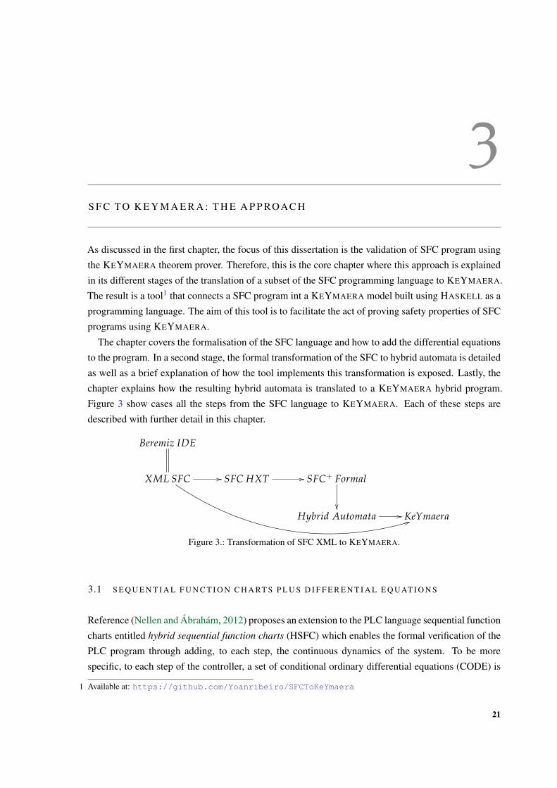
Figure 3 show cases all the steps from the SFC language to KEYMAERA. Each of these steps are
described with further detail in this chapter.
Beremiz IDE
XML SFC //
44
SFC HXT // SFC+ Formal
��Hybrid Automata // KeYmaera
Figure 3.: Transformation of SFC XML to KEYMAERA.
3.1 S E Q U E N T I A L F U N C T I O N C H A RT S P L U S D I F F E R E N T I A L E Q UAT I O N S
Reference (Nellen and Ábrahám, 2012) proposes an extension to the PLC language sequential function
charts entitled hybrid sequential function charts (HSFC) which enables the formal verification of the
PLC program through adding, to each step, the continuous dynamics of the system. To be more
specific, to each step of the controller, a set of conditional ordinary differential equations (CODE) is
1 Available at: https://github.com/Yoanribeiro/SFCToKeYmaera
21

Chapter 3. S F C T O K E Y M A E R A : T H E A P P R OAC H
added which models the behaviour of the continuous dynamics when the controller is in the specific
step in which the condition holds.
Firstly, it is necessary to define the formal syntax of the SFC language and fix the semantics since
"the semantics of SFCs given in IEC 61131-3 is ambiguous and erroneous, and PLC programming
tool developers interpret the ambiguities posed by the standard in different ways, which results in a
variety of different tool semantics" (Bauer et al., 2004).
3.1.1 SFC Syntax
The SFC syntax is defined by a set of variables which is the union of the input, output and local
variables of the program. Then, there is a set of steps and, connecting them, there is a set of guarded
transitions. A particular element of set S is initially active, i.e. the initial step. A particular transition is
taken if and only if the source step is active and the guard evaluates to true, this triggers immediately2
the inactivation of the source step and activation of the target step. Let GV be the set of guards over
the variables, which evaluates to true or false whenever the values of the variables are updated. There
is also a kind of transition which connects multiple sources/target which are the parallel branching.
Each step has a set of action blocks which indicates what must be performed upon activation. An
action block b = (q, a) is a pair with a qualifier q and an action a. The qualifier specifies when
the action must be performed, q ∈ {entry, do, exit}. In the IEC standard entry corresponds to the
qualifier P1 which is executed only the first time the step is activated, do represents the N qualifier
which is performed every time the step is activated and the exit qualifier is the P0 which is executed at
the deactivation of the step. There are other qualifiers which can be formally represented, however, in
this dissertation, they will not be considered. Similarly, an action a can only be a variable assignment,
even if it can be another SFC program. The history flag determines if the SFC program has memory,
in the case it does, in each execution cycle, the step which is activated is the step that was active in the
last cycle, otherwise, each execution cycle starts with its initial step. Formally,
Definition 2 (SFC syntax). A SFC program consists of a tuple
C = (V, S, A, s0, T, block,<,≺, Hist)
where
• V is a finite set of variables;
• S is a finite set of steps;
• A is a finite set of actions referring to variables in V in assignment and to SFCs whose variable
and actions sets are susbsets of V and A respectively,
• s0 ∈ S: represents the initial step;
2 Whenever the controller activates
22

3.1. Sequential Function Charts plus Differential Equations
• T ⊆ (2S \ {∅})× GV × (2S \ {∅}) is a finite set of transitions with multiple target/source
which define the begin/end of parallel branching;
• block : S→ 2BA is a function which assigns a set of action blocks to each step;
• < ⊆ A× A is a total order on actions;
• ≺ ⊆ T × T is a partial order on transitions;
• Hist ∈ 0, 1 is a history flag: if equal to 1 then the SFC program has active history.
3.1.2 SFC semantics
Programs running on a PLC follows these steps cyclically:
1. Checks the environment and obtains the input data which triggers the update of the values of
the variables.
2. Verifies the transitions that have to be taken and executes them.
3. Executes the actions accordingly in their priority order.
4. Sends the data to the output variable.
There is a time delay between two PLC cycles, this can be different for every other cycle, however,
the delay is delimited by a lower bound δt and an upper bound δu. The first and last step of the PLC
cycle define the communication with the environment; the remaining steps require the definition of
states and configurations. For a given SFC program E = (V, S, A, s0, T, block,<,≺, Hist), with Ddenoting the union of all type domains, a state σ ∈ Σ of E is a function σ : V → D which assigns a
value from its respective domain to each variable v ∈ V. The state transformation is also a function
f : Σ→ Σ. Then, a configuration is defined as (σ, readyS, activeS, activeA) ∈ Σ× S× S× A: the
state of the SFC, the set of ready steps; the set of active steps, the set of active actions which is sorted
by the ≺ relation.
Con f ig defines the set of configurations and the initial configuration of an SFC is defined by
(σ0, {s0}, ∅, ∅). For a SFC E and the configuration e = (σ, readyS, activeS, activeA) of E the
sets of enabled and taken transition are defined as:
enabled(E, e) = { (s, g, s′) ∈ T | s ⊆ activeS ∧ c |= g }taken(E, e) = { t = (s, g, s′) ∈ enabled(E, e) | ∀t1=(s1,g1,s1)∈enabled(E,e) • s ∩ s1 = ∅ ∨ t1 ≺ t }
This semantics focuses on computation steps inbetween the first and last step of the PLC cy-
cle: computation steps start with a configuration (σ, readyS, activeS, activeA) where σ was already
23
Chapter 3. S F C T O K E Y M A E R A : T H E A P P R OAC H
updated with new input data from the environment. The computation of the new configuration
(σ′, readyS′, activeS′, activeA′) is the result of executing the steps 2 and 3 of the PLC cycle. And
lastly, the output is sent to the environment. If the source step of all taken transitions is replaced by
the target step of those transitions afterwards, the new set of ready states is obtained. The new set of
active steps and active actions are then recursively calculated by the function computeActiveSets.
Definition 3 (SFC Semantics). Let S be a SFC without actions with nested SFC. The transition rela-
tion→⊆ Con f ig× Con f ig relates configurations
(σ, readyS, activeS, activeA)→ (σ′, readyS′, activeS′, activeA′)
as follows:
• readyS′ = (readyS \ source(taken(C, c)) ∪ target(taken(C, c)),
• (activeS′, unsortedActiveA′) = computeActiveSets(readyS′, ∅, ∅, C, c, ActivA)
• activeA′ = sort(unsortedActiveA′,<) and
• σ′ = (a1. . . . .am)(σ) where activeA′ = am. . . . .a1
The definition of the computeActiveSets can be found in the paper (Nellen and Ábrahám, 2012)
and all definition of the semantics and syntax are all excellently described and explained in (Bauer
et al., 2004).
3.1.3 Conditional ordinary differential equations
Conditional differential equation, CODE, are the ODEs which models the behaviour of the environ-
ment in which the programmable logic controller is. In (Nellen and Ábrahám, 2012) a Conditional
ODE is defined:
Definition 4 (Conditional ODE System). Let ODEVc be the set of all ordinary differential equations
over Vc (Vc is the set of continuous variables), and Conds, the set of all conditions. A conditional
ODE system consists of a pair (ODEs, cond) where cond ∈ Conds and ODEs ⊆ ODEVc . The set
of all conditional ODE system over Vc is denoted by CODEVc
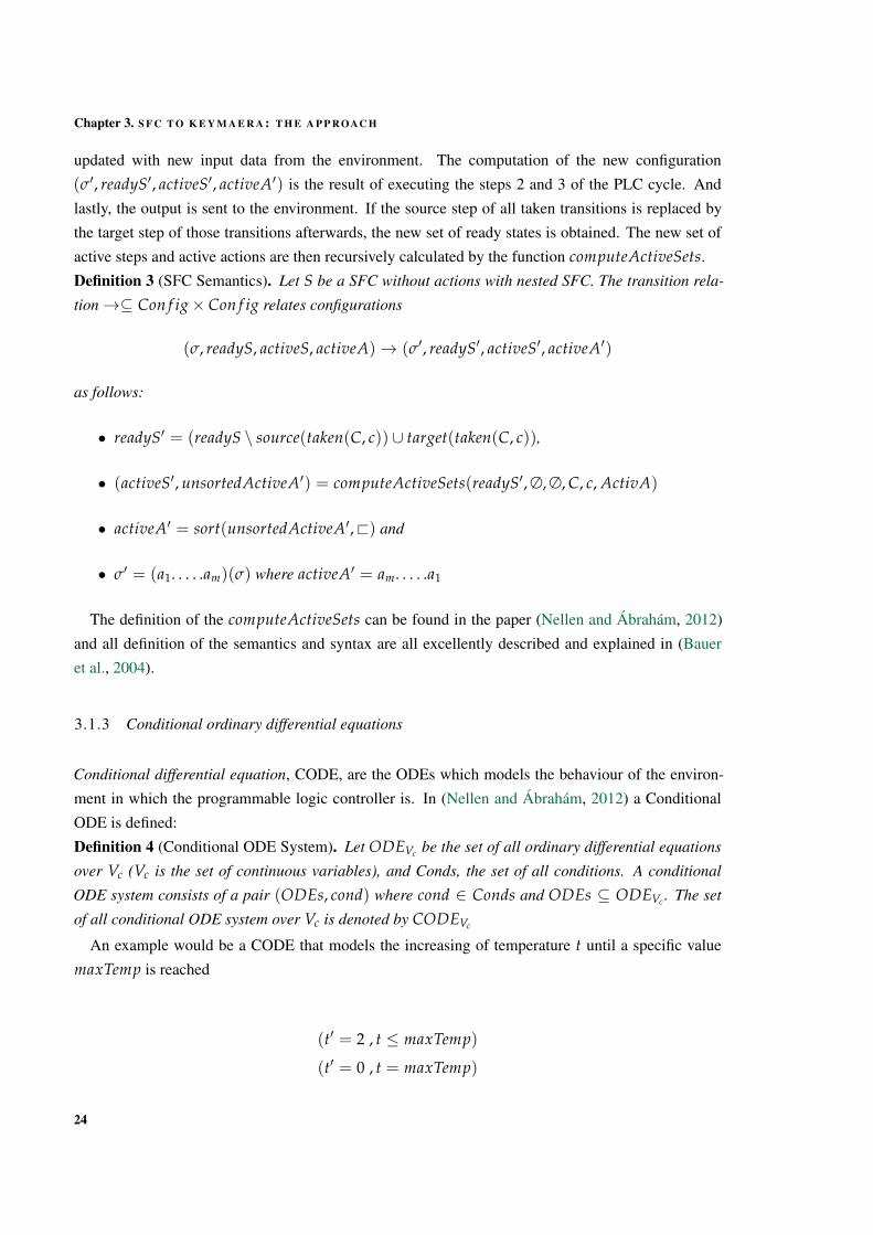
An example would be a CODE that models the increasing of temperature t until a specific value
maxTemp is reached
(t′ = 2 , t ≤ maxTemp)
(t′ = 0 , t = maxTemp)
24
3.2. Beremiz SFC to Haskell SFC
3.2 B E R E M I Z S F C T O H A S K E L L S F C
After programming a SFC program in the IDE Beremiz, the program can be compiled to C code
using the Matiec compiler, however what unifies the majority of the IDEs used by the IEC standard is
the XML representation given by PLCOpen3. It enables the exchange of programs, libraries, project
between IDEs. Therefore, the tool uses as input the XML file which contains the POU to verify.
3.2.1 SFCHXT
The component of the tool that is responsible for parsing the input resorts to the Haskell XML Toolbox
(HXT) library. The tool is responsible for parsing the file and obtaining the SFC structure in the form
of a Haskell data record. Firstly, however, it is created an intermediate structure called SFCHXT
(Appendix B) which is basically the representation of the XML constructs in Haskell, thus simplifying
the parsing process. After obtained, the SFCHXT structure, is transformed by the tool into its formal
SFC structure (Appendix C) to proceed to the translation to an hybrid automaton.
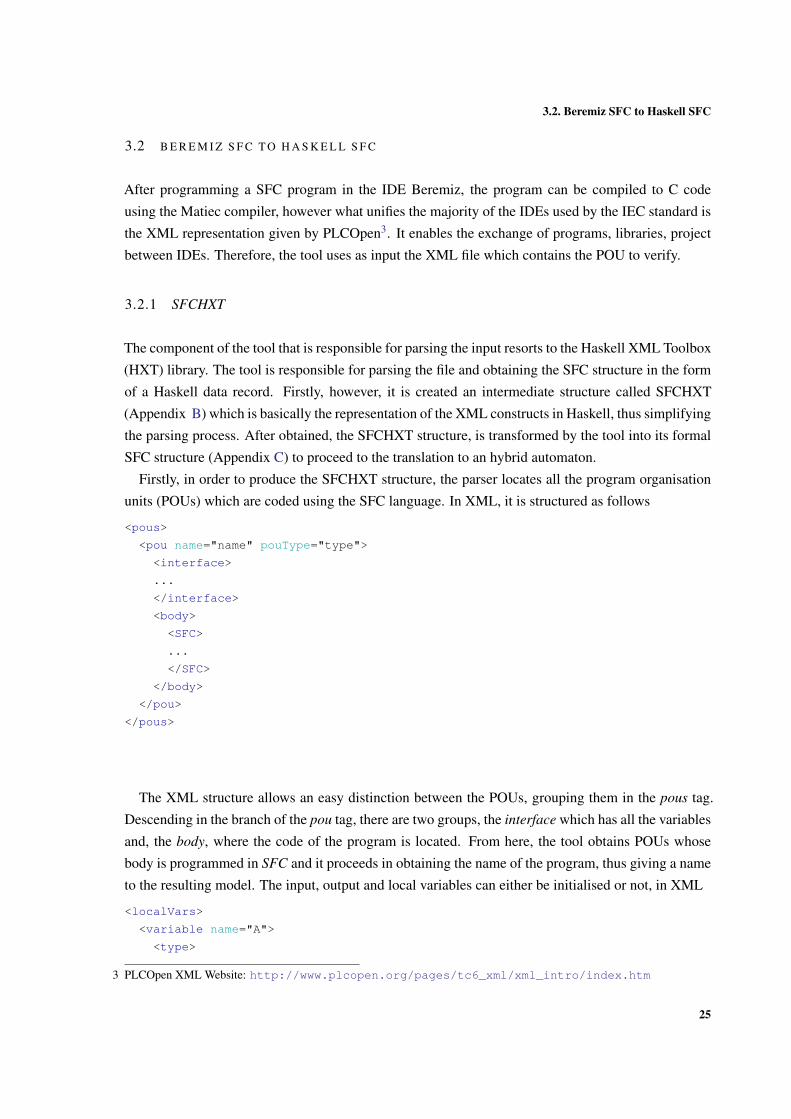
Firstly, in order to produce the SFCHXT structure, the parser locates all the program organisation
units (POUs) which are coded using the SFC language. In XML, it is structured as follows
<pous>
<pou name="name" pouType="type">
<interface>
...
</interface>
<body>
<SFC>
...
</SFC>
</body>
</pou>
</pous>
The XML structure allows an easy distinction between the POUs, grouping them in the pous tag.
Descending in the branch of the pou tag, there are two groups, the interface which has all the variables
and, the body, where the code of the program is located. From here, the tool obtains POUs whose
body is programmed in SFC and it proceeds in obtaining the name of the program, thus giving a name
to the resulting model. The input, output and local variables can either be initialised or not, in XML
<localVars>
<variable name="A">
<type>
3 PLCOpen XML Website: http://www.plcopen.org/pages/tc6_xml/xml_intro/index.htm
25

Chapter 3. S F C T O K E Y M A E R A : T H E A P P R OAC H
<TYPE1/>
</type>
</variable>
<initialValue>
<simpleValue value="val"/>
</initialValue>
</localVars>
<inputVars>
<variable name="B">
<type>
<TYPE2/>
</type>
</variable>
</inputVars>
<outputVars>
<variable name="C">
<type>
<TYPE3/>
</type>
</variable>
</outputVars>
The type of the variable must be restricted, since the variables used in hybrid automata and KEY-
MAERA are real numbers. This implies that the types allowed are integers, reals and booleans.
After obtaining the variables, the tool starts exploring the content of the SFC tag, since these ele-
ments are inside the body tag the type created was a BodyElem which is described in the Appendix B
The first step is to obtain the steps of the program. In XML, these are structured as
<step localId="id" name="nameStep" initialStep="value" height="x" width="y">
<connectionPointIn>
<connection refLocalId="refId"/>
</connectionPointIn>
</step>
The tool creates a BodyElem with type step which stores the localId if the step is a target the refId
corresponds to the component that is connected to this step.
After collecting all the steps, the actions are the next component of the SFC program to be collected
by the tool, these are structured as follows
<actionBlock localId="id" height="valHeight" width="valWidth">
<position x="valx0" y="valy0"/>
<connectionPointIn>
26

3.2. Beremiz SFC to Haskell SFC
<relPosition x="valx1" y="valx1"/>
<connection refLocalId="refId">
...
</connection>
</connectionPointIn>
<action localId="refId1" qualifier="qual">
<relPosition x="valx2" y="valy2"/>
<inline>
<ST>
<xhtml:p><![CDATA[action]]></xhtml:p>
</ST>
</inline>
</action>
</actionBlock>
Each action block has the refLocalId referring to the step where this action block is executed. The
action tag has the instruction which has to be performed and, the attribute qualifier, informs whether
the action is to be executed the first time the step is activated (P1), every time the step is activated (N),
or when this step is exited (P0).
Finally, the last component of the SFC to be dealt with are the transitions. These can be grouped in
three categories: the simple transitions, the divergence transitions and the convergence transition.
The simple transition is the component that contains the condition and a specific source and target.
The divergence selection and the convergence selection allows respectively a source to have multiple
targets and a target to have multiple sources.
<transition localId="id" height="valHeight" width="valWidth">
<position x="valx0" y="valy0"/>
<connectionPointIn>
<relPosition x="valx1" y="valy1"/>
<connection refLocalId="refID">
...
</connection>
</connectionPointIn>
<connectionPointOut>
...
</connectionPointOut>
<condition>
<inline name="">
<ST>
<xhtml:p><![CDATA[cond]]></xhtml:p>
</ST>
</inline>
</condition>
</transition>
27

Chapter 3. S F C T O K E Y M A E R A : T H E A P P R OAC H
The important information to extract from the transition is its own identifier, the refLocalId which
refers to its source and the condition in which the transition is taken.
<selectionConvergence localId="id" height="valHeight" width="valWidth">
<position x="valx1" y="valy1"/>
<connectionPointIn>
<relPosition x="valx1" y="valy1"/>
<connection refLocalId="refId1">
...
</connection>
</connectionPointIn>
<connectionPointIn>
<relPosition x="val2x" y="valy2"/>
<connection refLocalId="refId2">
...
</connection>
</connectionPointIn>
<connectionPointOut>
...
</connectionPointOut>
</selectionConvergence>
In the selectionConvergence tag, the identifier of the component must be stored and all the refLo-
calId of all the connected transitions. In the example they are refId1 and refId2.
<selectionDivergence localId="id" height="valHeight" width="valWidth">
<position x="valx0" y="valy0"/>
<connectionPointIn>
<relPosition x="valx1" y="valy1"/>
<connection refLocalId="refId">
...
</connection>
</connectionPointIn>
<connectionPointOut formalParameter="">
<relPosition x="valx2" y="valy2"/>
</connectionPointOut>
<connectionPointOut formalParameter="">
<relPosition x="valx3" y="valy3"/>
</connectionPointOut>
</selectionDivergence>
28

3.3. SFC annotation
Similarly, in the selectionDivergence, the identifier of the component and the refLocalId must be
stored, since the first will be referred in a number of transitions which diverge from this component
and the second is the source of all of those transitions.
The last important component is the comments since they contain the annotations that enrich the
SFC program.
<comment localId="id" height="valHeight" width="valWidth">
<position x="valx" y="valy"/>
<content>
<xhtml:p><![CDATA[annotation]]></xhtml:p>
</content>
</comment>
After parsing the XML structure, the direct representation of the SFC is created, the tool transforms
the SFCHXT structure into its formal representation, in Haskell (see Appendix C).
3.3 S F C A N N OTAT I O N
When the representation of SFC in XML is translated to the Haskell representation of the language,
the next step is to parse the annotations. There are five kinds of annotations that extend the SFC
language in Beremiz IDE. Note that not all the annotations are necessary to create a model from the
program, however it may require some handmade tweaks in the resulting model for it to run properly
in KEYMAERA.
1. CODE Annotation : The name is self-explanatory, for each step the CODEs are annotated.
2. Init Annotation : The pre-conditions of program can be stated in this annotation.
3. Invariant Annotation : The expression that is invariant in every execution of the program should
be stated in this annotations.
4. ToProve Annotation : The expression stated here represents the post-condition of the program
or the property to prove.
5. Extra Annotation : These annotation are basically a shortcut that can be used to swap expres-
sions that will not be useful once the program is transformed in its model by an equivalent
expression.
29
Chapter 3. S F C T O K E Y M A E R A : T H E A P P R OAC H
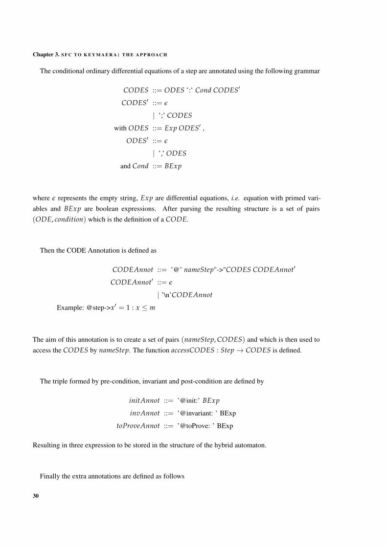
The conditional ordinary differential equations of a step are annotated using the following grammar
CODES ::= ODES ’:’ Cond CODES′
CODES′ ::= ε
| ’;’ CODES
with ODES ::= Exp ODES′ ,
ODES′ ::= ε
| ’,’ ODES
and Cond ::= BExp
where ε represents the empty string, Exp are differential equations, i.e. equation with primed vari-
ables and BExp are boolean expressions. After parsing the resulting structure is a set of pairs
(ODE, condition) which is the definition of a CODE.
Then the CODE Annotation is defined as
CODEAnnot ::= ’@’ nameStep"->"CODES CODEAnnot′
CODEAnnot′ ::= ε
| ’\n’CODEAnnot
Example: @step->x′ = 1 : x ≤ m
The aim of this annotation is to create a set of pairs (nameStep, CODES) and which is then used to
access the CODES by nameStep. The function accessCODES : Step→ CODES is defined.
The triple formed by pre-condition, invariant and post-condition are defined by
initAnnot ::= ’@init:’ BExp
invAnnot ::= ’@invariant: ’ BExp
toProveAnnot ::= ’@toProve: ’ BExp
Resulting in three expression to be stored in the structure of the hybrid automaton.
Finally the extra annotations are defined as follows
30

3.4. From SFC annotated to Hybrid Automata
extraAnnot ::= ’@Extras:\n’ swapBExp extraAnnot′
extraAnnot′ ::= ε
| swapBExp extraAnnot′
swapBExp ::= BExp ’:’ BExp
This results in set of pair (oldExp, newExp).
3.4 F RO M S F C A N N OTAT E D T O H Y B R I D AU T O M ATA
After defining the annotation language, the next step is the transformation of the annotated SFC to
Hybrid automata. This process has two steps which are based in Hybrid SFC (Nellen and Ábrahám,
2012).
1. Transform the pure SFC program into Hybrid Automata;
2. Adapt HA of step 1 with the CODEs resulting in the final HA.
As already stated in the previous section, CODEs are annotated in the SFC program using comments
of the Beremiz IDE. Moreover, there are other types of annotation which are relevant for the resulting
model in KEYMAERA.
3.4.1 From SFC to Hybrid Automaton
The SFC transformation to hybrid automaton consists of the following elements:
1. Each step of the SFC program corresponds to a location of the hybrid automaton.
2. The initial state of the HA is the initial step.
3. A clock variable is introduced, denominated t, which specifies the duration between two PLC
cycles; This implies that t must be bounded δl ≤ t ≤ δu.
4. An invariant t ≤ δu is added to every location to force the automaton to leave the location at
time δu at the latest.
5. No transition can be taken, before δl; then the guard t ≥ δl is added to all the transitions.
6. When a transition is taken the clock variable is reset.
31
Chapter 3. S F C T O K E Y M A E R A : T H E A P P R OAC H
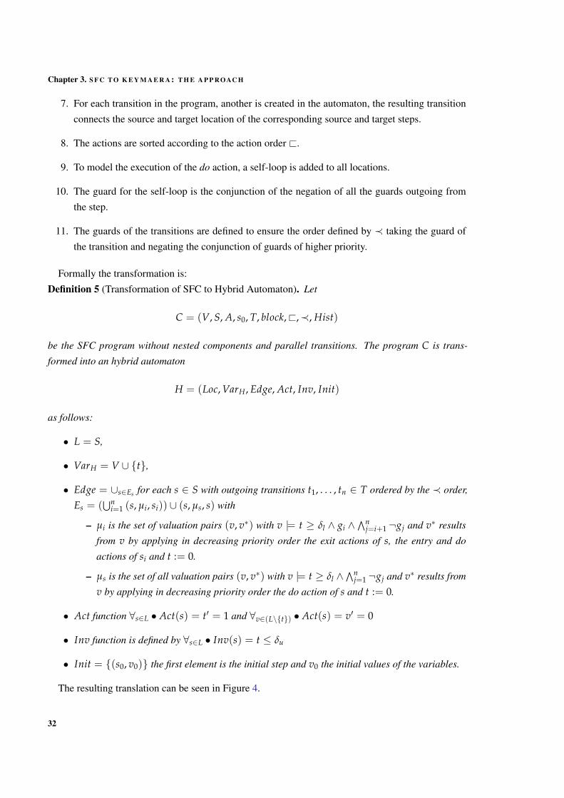
7. For each transition in the program, another is created in the automaton, the resulting transition
connects the source and target location of the corresponding source and target steps.
8. The actions are sorted according to the action order <.
9. To model the execution of the do action, a self-loop is added to all locations.
10. The guard for the self-loop is the conjunction of the negation of all the guards outgoing from
the step.
11. The guards of the transitions are defined to ensure the order defined by ≺ taking the guard of
the transition and negating the conjunction of guards of higher priority.
Formally the transformation is:
Definition 5 (Transformation of SFC to Hybrid Automaton). Let
C = (V, S, A, s0, T, block,<,≺, Hist)
be the SFC program without nested components and parallel transitions. The program C is trans-
formed into an hybrid automaton
H = (Loc, VarH, Edge, Act, Inv, Init)
as follows:
• L = S,
• VarH = V ∪ {t},
• Edge = ∪s∈Es for each s ∈ S with outgoing transitions t1, . . . , tn ∈ T ordered by the ≺ order,
Es = (⋃n
i=1 (s, µi, si)) ∪ (s, µs, s) with
– µi is the set of valuation pairs (v, v∗) with v |= t ≥ δl ∧ gi ∧∧n
j=i+1 ¬gj and v∗ results
from v by applying in decreasing priority order the exit actions of s, the entry and do
actions of si and t := 0.
– µs is the set of all valuation pairs (v, v∗) with v |= t ≥ δl ∧∧n
j=1 ¬gj and v∗ results from
v by applying in decreasing priority order the do action of s and t := 0.
• Act function ∀s∈L • Act(s) = t′ = 1 and ∀v∈(L\{t}) • Act(s) = v′ = 0
• Inv function is defined by ∀s∈L • Inv(s) = t ≤ δu
• Init = {(s0, v0)} the first element is the initial step and v0 the initial values of the variables.
The resulting translation can be seen in Figure 4.
32

3.4. From SFC annotated to Hybrid Automata
. . .
. . .
P1 entryN doP0 exit
Step
g1 gn
Step1 Stepn
. . .
. . .
s
t ≤ δut′ = 1
s1
. . .
sn
. . .
t ≥ δl ∧ g1exit(s); entry(s1); do(s1); t := 0
t ≥ δl ∧ gn ∧∧n−1
i=1 ¬giexit(s); entry(sn); do(sn); t := 0
t ≥ δl∧n
i=1 ¬gido(s); t := 0
Figure 4.: Transformation SFC to Hybrid Automaton.
3.4.2 From SFCs and CODES to Hybrid Automaton
Once the SFC is translated to an hybrid automaton, the next stage of the translation is to create the final
hybrid automaton. Firstly, the set CODES is obtained from parsing the annotations SCODES and its
respective function accessCODES. Then for each step, s ∈ S with CODEs {(ODE1, c1), . . . , (ODEn, cn)},the location resulting from the first transformation is replaced by n + 1 copies s1, . . . , sn+1; the invari-
ant of each of these copies i = 1, . . . , n is defined by ci ∧∧i−1
j=1 ¬cj; the ODE of each of the copies
is given by ODEi. To the invariant of the n + 1 copy is added the expression∧n
j=1 ¬cj. There must
be two transitions between each two copies si and sj, i 6= j, to enable the switching from one copy to
another when the evaluation of the conditions changes, the results can be seen in Figure 5
S @S− > ODE1:c1;...;ODEn:cn
s1...
ODE1
c1
...
sn...
ODEn
cn
Figure 5.: Adaptation of annotated step to Hybrid automaton.
Definition 6 (Transformation of SFC with CODEs to Hybrid Automaton). Let
C = (V, S, A, s0, T, block,<,≺, Hist)
33

Chapter 3. S F C T O K E Y M A E R A : T H E A P P R OAC H
be a SFC program without nested components and parallel transitions. The program C is transformed
into an hybrid automaton
H = (Loc, VarH, Edges, Act, Inv, Init)
together with a set of CODES = {(S, CODES)}, the respective function accessCODES and the set
of continuous variables Vc, defined as follows:
• Loc =⋃
s∈S Ls with Ls = {si | 1 ≤ i ≤ (#(accessCODES(s)) + 1)},
• VarH = V ∪Vc ∪ {t},
• For each step s ∈ S with accessCODES(s) = {(ODE1, cond1), . . . , (ODEm, condm)} and
outgoing transitions t1, . . . , tn ∈ T ordered by ≺ E =
– For each sk ∈ Ls there is an edge (sk, µ, sk) with µ the set of all (v, v∗) with v |= t ≥δl ∧
∧nj=1 ¬gj and v∗ the result from v by applying the ordered sequence of do actions of
s plus t := 0.
– For all sk, sl ∈ LS, sk 6= sl there are edges (sk, µ, sl) and (sl , µ, sk) with µ the identity
relation.
• Act function ∀s∈S, accessStep(s) = {(ODE1, cond1), . . . , (ODEm, condm)}∧ Ls = {s1, . . . , sm+1} •Act(si) = ODEi ∪ t′ = 1, i = 1, . . . , m and Act(sm+1) = t′ = 1
• Inv function ∀s∈S, accessStep(s) = {(ODE1, cond1), . . . , (ODEm, condm)}∧ Ls = {s1, . . . , sm+1} •Inv(si) = condi ∧ (
∧i−1j=1 ¬condj)∧ t ≤ δu, i = 1, . . . , m and Inv(sm+1) = (
∧mj=1 ¬condj)∧
t ≤ δu
• Init = {(s0, v0)} the first element is the initial step and v0 the initial values of the variables.
3.5 H Y B R I D AU T O M ATA T O K E Y M A E R A
The final transformation that must be done to conclude the transformation is to represent the HA in
a hybrid program for KEYMAERA. This is easily done since a hybrid automata can be represented
naturally as a hybrid program once the second is a representation of the first (Platzer, 2010).
Considering the HA H = (V, L, E, I, F, init) and the initCond, toProveandcycleInv. For the re-
sulting HP, all the variables of V are declared in the programVariable environment together with a
variable st representing the state in the automaton; the delays of SFC are represented as f unctionsenvironment. The model is defined as follows:
(initCond ∧ 0 < δl ∧ 0 < δu ∧ δl < δu)[initVariables](st = init→ [φ](postCondition))
34

3.5. Hybrid Automata to KeYmaera
The initCond and postCondition are obtained by the annotation. The initVariables is basically
the attribution of the value in which each variables is initialised. The st = initState is an abuse of
notation since the init is a location init ∈ L a st ∈ R. The φ program is defined as:
∀l∈L∧e1,...,em∈{e′|source(e)=l}•?(st = l);
?(cond(e1));
event(e1);
st := target(e1)
∪. . .
∪?(cond(en));
event(en);
st := target(en)
∪{ f low(l), inv(l)}
The functions source and target return the source and target of the transitions respectively; the
function cond is the function that, given an edge, returns the condition for the transitions to occur.
The event function gives back the set of assignments to be executed when the transitions is taken.
35


4
C A S E S T U DY: T H E WAT E R H E AT I N G TA N K
In Chapter 3, it is shown how the transformation from sequential function charts with annotations to
KEYMAERA was designed in order to implement a tool to prove safety properties of a SFC program.
The main aim of this chapter is to understand what is the actual extent of the implemented tool with
the support of a case study.
Though the water tank problem is a fairly usual (e.g (Platzer, 2010)) example used in the domain of
hybrid systems, it can be modified to a water heating tank, to further increment the complexity of the
problem. Firstly, the description of the problem is exposed, then the PLC program is designed and,
finally, the tool is used to obtain the model and prove some properties.
4.1 D E S C R I P T I O N O F T H E P RO B L E M
Consider an empty tank. The goal of this system is to heat the temperature of the water to be used in
some other task. The tank has to be fully filled and only then the controller starts the heating process.
After a while, the tank is again emptied and the process starts over.
To implement this tank, it must have a sensor which detects that it is empty giving a Empty signal.
However, the process only begins once the Start signal is given. Once both signals are received the
discharge valve is closed and the filling pump is activated. When the sensor detects that the tank is
full, Full signal is sent and the filling pump is stopped. Consequently, the heater is switched on. When
the sensors reads 90 degrees Celsius, the heater is switched off and a timer is set to 20 minutes. Once
the timer reaches 20 minutes, the controller opens the discharge valve and begin the emptying process.
Finally, when the water-tank is empty, the process begins anew.
The filling process begins and its dynamics is described by the differential equations that give the
height of the water, namely, y′ = 3. When the heater is on the differential equations that describes
its behaviour is give by temp′ = 4 knowing that the temperature of the water starts at 20 degrees
Celsius, and finally, once the controller opens the discharge valve the height of the water is given by
the equation y′ = −4.
The safety property that the program must guarantee throughout the all execution of the PLC pro-
gram is that the water level is always between Empty and Full signals.
37

Chapter 4. C A S E S T U DY: T H E WAT E R H E AT I N G TA N K
4.2 T H E S F C P RO G R A M A N D T H E G E N E R AT E D M O D E L
4.2.1 Program and annotations
From the description of the problem, the type of variables we need to declare can be easily identified.
1. The signal variables, which must be of type boolean, to represent whether a sensor or a other
controller is activated or not.
2. The quantified variables, of type real (R), represent a "sensor" which outputs real values.
The signal variables are Empty, Start, Full, the discharge valve (dv), the pump and the heater. The
quantified variables are the timer tm′ and the temperature temp.
The steps of the program are deduced from the states of the system. Therefore for this specific
program the steps are:
• Step1 represents the empty tank;
• Step2 represents the filling process;
• Step3 represents the heating process;
• Step4 represents the waiting process;
• Step5 represents the emptying process.
With respect to the actions of this program, every action has, as quantifier, P1 since they are all
executed only at the first time the step is activated. There is no actions to be executed on Step1;
on Step2 the discharge variable evaluates to f alse and the pump to true; on Step3 the pump variable
evaluates to f alse and the heater variable to true; the actions in Step4 are the deactivation of the heater
variable and the assignment to the timer 20 min; finally the last step activates discharge variable.
The transitions are the last components to be defined:
• From Step1 to Step2 Empty = True ∧ Start = True must hold.
• From Step2 to Step3 Full = True must hold.
• From Step3 to Step4 temp = 90 must hold.
• From Step4 to Step5 tm = 20 must hold.
• From Step5 to Step1 Empty = True must hold.
Formally, SFC water heating tank program is illustrated in Figure 6. The water heating tank consists
of the SFC C = (V, S, A, s0, T, block,<,≺, Hist) with
38
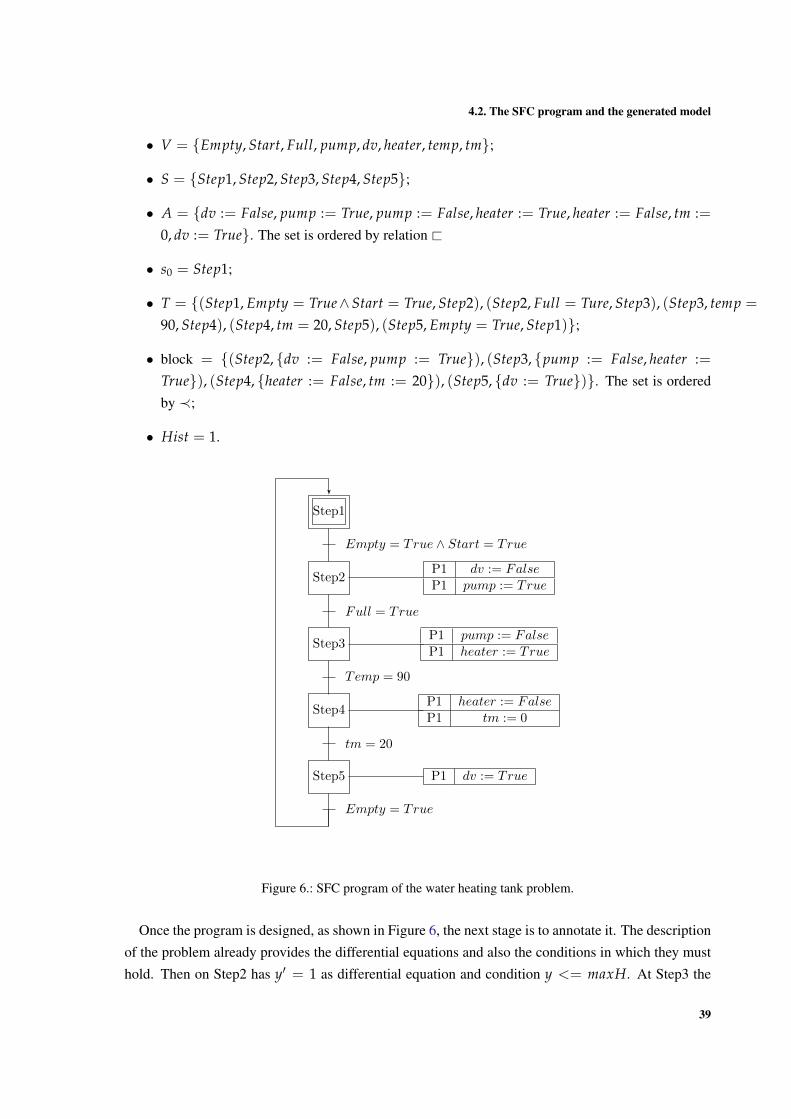
4.2. The SFC program and the generated model
• V = {Empty, Start, Full, pump, dv, heater, temp, tm};
• S = {Step1, Step2, Step3, Step4, Step5};
• A = {dv := False, pump := True, pump := False, heater := True, heater := False, tm :=0, dv := True}. The set is ordered by relation <
• s0 = Step1;
• T = {(Step1, Empty = True∧Start = True, Step2), (Step2, Full = Ture, Step3), (Step3, temp =
90, Step4), (Step4, tm = 20, Step5), (Step5, Empty = True, Step1)};
• block = {(Step2, {dv := False, pump := True}), (Step3, {pump := False, heater :=True}), (Step4, {heater := False, tm := 20}), (Step5, {dv := True})}. The set is ordered
by ≺;
• Hist = 1.
Step1
Empty = True ∧ Start = True
Step2
Full = True
Step3
Temp = 90
Step4
tm = 20
Step5
Empty = True
P1 dv := FalseP1 pump := True
P1 pump := FalseP1 heater := True
P1 heater := FalseP1 tm := 0
P1 dv := True
Figure 6.: SFC program of the water heating tank problem.
Once the program is designed, as shown in Figure 6, the next stage is to annotate it. The description
of the problem already provides the differential equations and also the conditions in which they must
hold. Then on Step2 has y′ = 1 as differential equation and condition y <= maxH. At Step3 the
39

Chapter 4. C A S E S T U DY: T H E WAT E R H E AT I N G TA N K
system dynamics is given by the set of ODEs y′ = 0 and temp′ = 2 and the temp ≤ 90 must hold
for the second ODE. Step4 has tm′ = 1 and temp′ = 0 as ODES describing its dynamics and the
condition tm ≤ 20 must be true for the first equation. At Step5 tm′ = 0 and y′ = −2 describes the
dynamics of the system and y ≥ 0 must be true for the second differential equation.
The precondition, invariant and postconditions are, respectively, maxH > 0∧ 0 <= y <= maxH.
The remaining conditions are 0 <= y <= maxH. Note that, for the extra annotation, it is necessary
to locate the conditions which are not coherent once the program is translated. These conditions are
Full = True and Empty = True, consequently these must be substituted by y = maxH and y = 0respectively. The use of maxH introduces an abstract ceiling for the height of the water, since the
maximum height was not in the description.
The resulting program in Beremiz can seen in figure 7
Figure 7.: Water heating tank program with annotation in Beremiz IDE.
The resulting XML file (see appendix E) is then given to the tool to generate the model and the tool
returns the message seen on Figure 8
Figure 8.: The resulting message given by the tool after processing the PLC program.
40

4.2. The SFC program and the generated model
4.2.2 Model obtained
The resulting model is quite large since the program has five steps and four of them have two CODE
each. Thus,
\functions{
R deltaCycleMin;
R deltaCycleMax;
}
\programVariables {
R Empty;
R Full;
R Start;
R dv;
R heater;
R maxH;
R pump;
R t;
R temp;
R tm;
R y;
R st;
}
/**Step2:0
Step20:1
Step3:2
Step30:3
Step31:4
Step4:5
Step40:6
Step41:7
Step5:8
Step50:9
Step51:10
Step1:11
**/
\problem {
(
(
maxH>0.0&y>=0.0&y<=maxH&
deltaCycleMin>0 & deltaCycleMax>0
&
deltaCycleMin < deltaCycleMax
)
->
\[
t:=0.0;
st:=11.0
\](
st=11
->
\[
(
(
?(st=0);
(
?(y=maxH);
(
pump := 0;heater :=
1;
st:=2
) ++
?(y=maxH);
(
pump := 0;heater :=
1;
st:=3
) ++
?(y=maxH);
(
pump := 0;heater :=
1;
st:=4
) ++
?(!(y=maxH));
(
st:=0
) ++
(
st:=1
) ++
{t’=1,t<=deltaCycleMax
,!(y<=maxH)}
)
)
++
41

Chapter 4. C A S E S T U DY: T H E WAT E R H E AT I N G TA N K
(
?(st=1);
(
?(y=maxH);
(
pump := 0;heater :=
1;
st:=2
) ++
?(y=maxH);
(
pump := 0;heater :=
1;
st:=3
) ++
?(y=maxH);
(
pump := 0;heater :=
1;
st:=4
) ++
?(!(y=maxH));
(
st:=1
) ++
(
st:=0
) ++
{y’=1.0,t’=1,y<=maxH,t<=
deltaCycleMax}
)
)
++
(
?(st=2);
(
?(temp=90);
(
heater := 0;tm := 0;
st:=5
) ++
?(temp=90);
(
heater := 0;tm := 0;
st:=6
) ++
?(temp=90);
(
heater := 0;tm := 0;
st:=7
) ++
?(!(temp=90));
(
st:=2
) ++
(
st:=3
) ++
(
st:=4
) ++
{t’=1,t<=deltaCycleMax
,!(temp<=90.0)}
)
)
++
(
?(st=3);
(
?(temp=90);
(
heater := 0;tm := 0;
st:=5
) ++
?(temp=90);
(
heater := 0;tm := 0;
st:=6
) ++
?(temp=90);
(
heater := 0;tm := 0;
st:=7
) ++
?(!(temp=90));
(
st:=3
) ++
(
st:=2
) ++
42
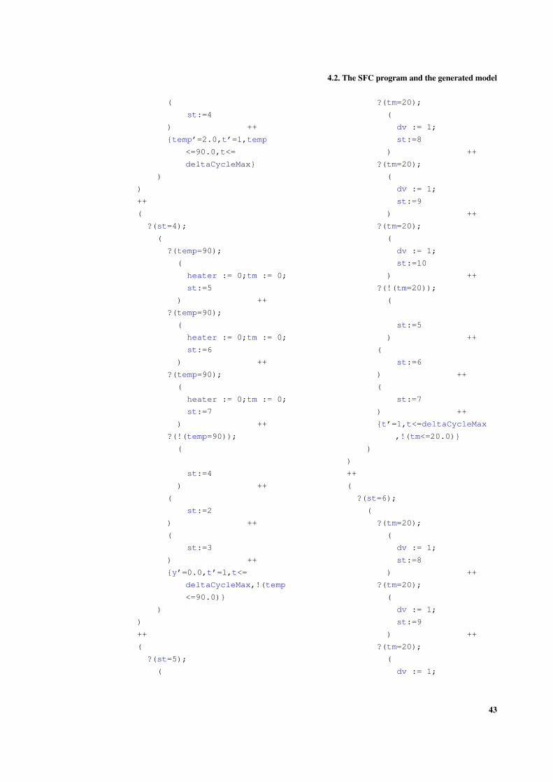
4.2. The SFC program and the generated model
(
st:=4
) ++
{temp’=2.0,t’=1,temp
<=90.0,t<=
deltaCycleMax}
)
)
++
(
?(st=4);
(
?(temp=90);
(
heater := 0;tm := 0;
st:=5
) ++
?(temp=90);
(
heater := 0;tm := 0;
st:=6
) ++
?(temp=90);
(
heater := 0;tm := 0;
st:=7
) ++
?(!(temp=90));
(
st:=4
) ++
(
st:=2
) ++
(
st:=3
) ++
{y’=0.0,t’=1,t<=
deltaCycleMax,!(temp
<=90.0)}
)
)
++
(
?(st=5);
(
?(tm=20);
(
dv := 1;
st:=8
) ++
?(tm=20);
(
dv := 1;
st:=9
) ++
?(tm=20);
(
dv := 1;
st:=10
) ++
?(!(tm=20));
(
st:=5
) ++
(
st:=6
) ++
(
st:=7
) ++
{t’=1,t<=deltaCycleMax
,!(tm<=20.0)}
)
)
++
(
?(st=6);
(
?(tm=20);
(
dv := 1;
st:=8
) ++
?(tm=20);
(
dv := 1;
st:=9
) ++
?(tm=20);
(
dv := 1;
43

Chapter 4. C A S E S T U DY: T H E WAT E R H E AT I N G TA N K
st:=10
) ++
?(!(tm=20));
(
st:=6
) ++
(
st:=5
) ++
(
st:=7
) ++
{tm’=1.0,t’=1,tm<=20.0,t
<=deltaCycleMax}
)
)
++
(
?(st=7);
(
?(tm=20);
(
dv := 1;
st:=8
) ++
?(tm=20);
(
dv := 1;
st:=9
) ++
?(tm=20);
(
dv := 1;
st:=10
) ++
?(!(tm=20));
(
st:=7
) ++
(
st:=5
) ++
(
st:=6
) ++
{temp’=0.0,t’=1,t<=
deltaCycleMax,!(tm
<=20.0)}
)
)
++
(
?(st=8);
(
?(y=0.0);
(
st:=11
) ++
?(!(y=0.0));
(
st:=8
) ++
(
st:=9
) ++
(
st:=10
) ++
{t’=1,t<=deltaCycleMax
,!(y>=0.0)}
)
)
++
(
?(st=9);
(
?(y=0.0);
(
st:=11
) ++
?(!(y=0.0));
(
st:=9
) ++
(
st:=8
) ++
(
44

4.3. Verifying safety properties
st:=10
) ++
{y’=-2.0,t’=1,y>=0.0,t<=
deltaCycleMax}
)
)
++
(
?(st=10);
(
?(y=0.0);
(
st:=11
) ++
?(!(y=0.0));
(
st:=10
) ++
(
st:=8
) ++
(
st:=9
) ++
{tm’=0.0,t’=1,t<=
deltaCycleMax,!(y
>=0.0)}
)
)
++
(
?(st=11);
(
?(y=0.0&Start=1);
(
pump := 1;dv := 0;
st:=0
) ++
?(y=0.0&Start=1);
(
pump := 1;dv := 0;
st:=1
) ++
?(!(y=0.0&Start=1));
(
st:=11
) ++
{t’=1,t<=deltaCycleMax}
)
) )*@invariant(
y>=0.0&y<=maxH
)
\](
y>=0.0&y<=maxH
)
)
)
}
4.3 V E R I F Y I N G S A F E T Y P RO P E RT I E S
The safety property to be proved in the model is that the height of the water has to remain between
Empty signal and Full signal i.e. y ≥ 0.0∧ y ≤ maxH. KEYMAERA proves it, as shown in Figure 9.
45
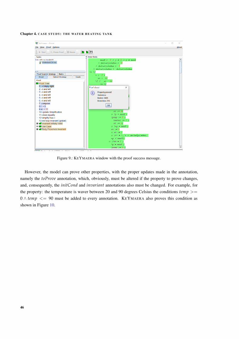
Chapter 4. C A S E S T U DY: T H E WAT E R H E AT I N G TA N K
Figure 9.: KEYMAERA window with the proof success message.
However, the model can prove other properties, with the proper updates made in the annotation,
namely the toProve annotation, which, obviously, must be altered if the property to prove changes,
and, consequently, the initCond and invariant annotations also must be changed. For example, for
the property: the temperature is waver between 20 and 90 degrees Celsius the conditions temp >=
0 ∧ temp <= 90 must be added to every annotation. KEYMAERA also proves this condition as
shown in Figure 10.
46

4.3. Verifying safety properties
Figure 10.: KEYMAERA window with the proof success message with the temperature condition.
Figure 11.: KEYMAERA window on an unsuccessful attempt to prove y = 0.
47

Chapter 4. C A S E S T U DY: T H E WAT E R H E AT I N G TA N K
Furthermore, consider how to prove that the model is not stationary, i.e. that the variables do
not always have the same value even with the correct precondition and invariant. Considering the
preconditions and invariant from the last model, the model cannot prove that the height of the water is
always zero. The condition does not hold because the invariant of the program does not imply that the
height is always equal to zero (see Figure 11). This allows to conclude that the model does not prove
the safety condition trivially, thus proving that the model is not stationary.
48

5
C A S E S T U DY: T H E P H P L A N T
This chapter discusses another case study on the use of KEYMAERA to verify SFC programs. The
case study is about a pH plant which is responsible by monitoring the pH of the water in a tank whilst
the latter is being filled.
Similarly to Chapter 4, the problem is first discribed in natural language. Then it is scrutinised to
obtain the different components to design the desired PLC program. Finally the tool is used to obtain
a corresponding hybrid program on top of which some properties of the controller can be proved.
5.1 D E S C R I P T I O N O F T H E P RO B L E M
Let us consider a water tank that is being filled. The aim of the controller is to monitor the pH level
of the water until the tank is completely full. The water pH can vary from normal, to low or high.
The controller must have a pH sensor, which provides the current value of the water pH, and a
sensor, which gives a full signal to halt the filling process. The controller can send signals to valves
which are responsible for introducing a treatment to decrease or increase the value of pH, the controller
can also send a signal to the pump to halt the filling process.
When acting to decrease the water pH, the controller state is given by the differential equation
ph′ = −0.7, which is active while the condition ph > 7.0 holds. When increasing the pH level, this
value is given by the equation ph′ = 0.9 and the treatment continues while the condition pH < 7.0holds. When the water has a neutral pH and since it is filling (causing an increase of the pH level)
the dynamics of the pH is given by the equation ph′ = 0.1 and, the pH level must stay between 6.8
and 7.2. The filling process dynamics is the same for all levels of pH and is given by the differential
equation y′ = 0.1, with the water height between 0 and 1 (0 ≤ y < 1).
The property which ensures the tank system is safe is that the tank does not overflow and the pH
level is always between 6.8 and 7.2
49

Chapter 5. C A S E S T U DY: T H E P H P L A N T
5.2 T H E S F C P RO G R A M A N D T H E G E N E R AT E D M O D E L
5.2.1 Program and annotations
After exposing the problem, the next stage is to extract the necessary components to design the SFC
program. Similarly to the water tank case study discussed in the previous chapter, there are two type
of variables, namely, the signal variables and the quantified variables. The first are the full signal given
when the water height maximum is reached, the pump signal responsible by the valve which fills the
tank, and the two valves to pump the treatment to decrease the pH level, vphm, or to increase it, the
vphp. The quantified variable is ph representing the sensor that shows the pH value.
The different steps of the program are the following:
• Step1 represents the water tank with neutral pH;
• Step2 represents the water tank with high pH (alkaline);
• Step3 represents the water tank with low pH (acidic);
• Step4 represents the full water tank.
The qualifier of every action in the PLC program is P1, entailing that they must be executed only at
the first time the step is activated. At Step1, both valves responsible for the treatment are closed, i.e.
the program sends the signal false to both variables. At Step2, the valve used to decrease the pH level
is opened, i.e. the program sends a true signal to the corresponding variable. At Step3, the valve for
increasing of the water pH is opened, i.e. true signal is sent to the corresponding variable. Finally at
Step4, the pump variable is set to false to stop the filling process.
Finally, the last component of this SFC program is the set of transitions:
• From Step1 to Step2 ph ≥ 7.2 must hold.
• From Step1 to Step3 ph ≤ 6.8 must hold.
• From Step1 to Step4 f ull = True must hold.
• From Step2 to Step4 f ull = True must hold.
• From Step2 to Step1 ph ≤ 7.0 must hold.
• From Step3 to Step4 f ull = True must hold.
• From Step3 to Step1 ph ≥ 7.0 must hold.
The SFC program is graphically represented in Figure 12.
Formally, it consists of the tuple C = (V, S, A, s0, T, block,<,≺, Hist), where
50

5.2. The SFC program and the generated model
• V = { f ull, vphp, vphm, pump, ph};
• S = {Step1, Step2, Step3, Step4};
• A = {vphp := False, vphm := False, vphm := True, vphp := True, pump := False} The
set is ordered by relation <
• s0 = Step1;
• T = {(Step1, ph ≥ 7.2, Step2), (Step1, ph ≤ 6.8, Step3), (Step1, f ull = True, Step4), (Step2, f ull =True, Step4), (Step2, ph ≤ 7.0, Step1), (Step3, f ull = True, Step4), (Step3, ph ≥ 7.0, Step1)};
• block = {(Step1, {vphp := False, vphm := False}), (Step2, {vphm := True}), (Step3, {vphp :=True}), (Step4, {pump := False})}. The set is ordered by relation ≺;
• Hist = 1.
Step1
ph ≥ 7.2 full = True ph ≤ 6.8
Step2
full = Trueph ≤ 7.0
Step3
full = True ph ≥ 7.0
Step4
P1 vphm := FalseP1 vphp := False
P1 vphm := True P1 vphp := True
P1 pump := False
Figure 12.: SFC program representing the pH plant problem.
After designing the SFC program, the step part of the process to obtain corresponding hybrid model
of the pH plant is to annotate the PLC program. Starting with the conditional differential equations
annotation, from Step1 to Step4 the equation which represents the dynamics of the water height is
y′ = 0.1 and the condition 0 ≤ y < 1 must hold. Then for Step1 the differential equation for the
dynamics of the pH level is given by ph′ = 0.1 and the condition 6.8 < ph < 7.2 must hold. For
Step2 the differential equation ph′ = −0.7 and the condition ph ≥ 7.0 must hold. For Step3 the
equation ph′ = 0.9 and the condition ph ≤ 7.0 must hold. Finally, for Step4 the relevant differential
equations are ph′ = 0 and y′ = 0.
The preconditions, invariants and postconditions are, respectively, 0 ≤ y ≤ 0.1 ∧ 7.05 ≤ ph ≤7.15 and the remaining two conditions are 0 ≤ y ≤ 1 ∧ 6.8 ≤ ph ≤ 7.2. For the extra annotation, it
51
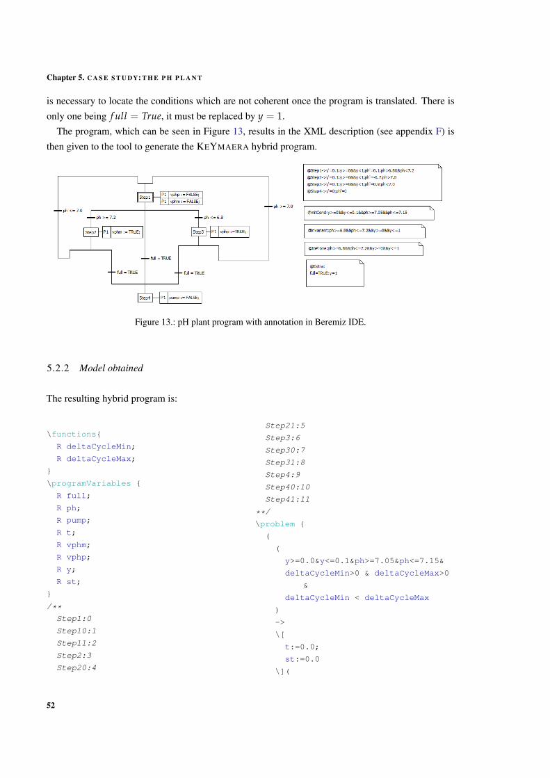
Chapter 5. C A S E S T U DY: T H E P H P L A N T
is necessary to locate the conditions which are not coherent once the program is translated. There is
only one being f ull = True, it must be replaced by y = 1.
The program, which can be seen in Figure 13, results in the XML description (see appendix F) is
then given to the tool to generate the KEYMAERA hybrid program.
Figure 13.: pH plant program with annotation in Beremiz IDE.
5.2.2 Model obtained
The resulting hybrid program is:
\functions{
R deltaCycleMin;
R deltaCycleMax;
}
\programVariables {
R full;
R ph;
R pump;
R t;
R vphm;
R vphp;
R y;
R st;
}
/**Step1:0
Step10:1
Step11:2
Step2:3
Step20:4
Step21:5
Step3:6
Step30:7
Step31:8
Step4:9
Step40:10
Step41:11
**/
\problem {
(
(
y>=0.0&y<=0.1&ph>=7.05&ph<=7.15&
deltaCycleMin>0 & deltaCycleMax>0
&
deltaCycleMin < deltaCycleMax
)
->
\[
t:=0.0;
st:=0.0
\](
52

5.2. The SFC program and the generated model
st=0
->
\[
(
(
?(st=0);
(
?(ph>=7.2&!(ph<=6.8)&!(y
=1.0));
(
vphm := 1;
st:=3
) ++
?(ph>=7.2&!(ph<=6.8)&!(y
=1.0));
(
vphm := 1;
st:=4
) ++
?(ph>=7.2&!(ph<=6.8)&!(y
=1.0));
(
vphm := 1;
st:=5
) ++
?(ph<=6.8&!(y=1.0));
(
vphp :=1;
st:=6
) ++
?(ph<=6.8&!(y=1.0));
(
vphp :=1;
st:=7
) ++
?(ph<=6.8&!(y=1.0));
(
vphp :=1;
st:=8
) ++
?(y=1.0);
(
pump := 0;
st:=9
) ++
?(y=1.0);
(
pump := 0;
st:=10
) ++
?(y=1.0);
(
pump := 0;
st:=11
) ++
?(!(ph>=7.2)&!(ph<=6.8)
&!(y=1.0));
(
st:=0
) ++
(
st:=1
) ++
(
st:=2
) ++
{t’=1,t<=deltaCycleMax
,!(y>=0.0&y<1.0),!(
ph>6.8&ph<7.2)}
)
)
++
(
?(st=1);
(
?(ph>=7.2&!(ph<=6.8)&!(y
=1.0));
(
vphm := 1;
st:=3
) ++
?(ph>=7.2&!(ph<=6.8)&!(y
=1.0));
(
vphm := 1;
st:=4
) ++
?(ph>=7.2&!(ph<=6.8)&!(y
=1.0));
(
vphm := 1;
st:=5
) ++
53
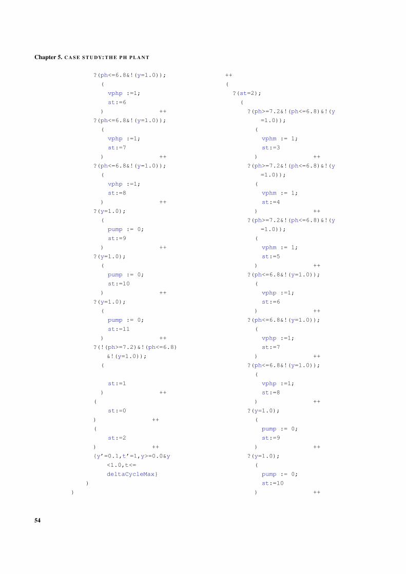
Chapter 5. C A S E S T U DY: T H E P H P L A N T
?(ph<=6.8&!(y=1.0));
(
vphp :=1;
st:=6
) ++
?(ph<=6.8&!(y=1.0));
(
vphp :=1;
st:=7
) ++
?(ph<=6.8&!(y=1.0));
(
vphp :=1;
st:=8
) ++
?(y=1.0);
(
pump := 0;
st:=9
) ++
?(y=1.0);
(
pump := 0;
st:=10
) ++
?(y=1.0);
(
pump := 0;
st:=11
) ++
?(!(ph>=7.2)&!(ph<=6.8)
&!(y=1.0));
(
st:=1
) ++
(
st:=0
) ++
(
st:=2
) ++
{y’=0.1,t’=1,y>=0.0&y
<1.0,t<=
deltaCycleMax}
)
)
++
(
?(st=2);
(
?(ph>=7.2&!(ph<=6.8)&!(y
=1.0));
(
vphm := 1;
st:=3
) ++
?(ph>=7.2&!(ph<=6.8)&!(y
=1.0));
(
vphm := 1;
st:=4
) ++
?(ph>=7.2&!(ph<=6.8)&!(y
=1.0));
(
vphm := 1;
st:=5
) ++
?(ph<=6.8&!(y=1.0));
(
vphp :=1;
st:=6
) ++
?(ph<=6.8&!(y=1.0));
(
vphp :=1;
st:=7
) ++
?(ph<=6.8&!(y=1.0));
(
vphp :=1;
st:=8
) ++
?(y=1.0);
(
pump := 0;
st:=9
) ++
?(y=1.0);
(
pump := 0;
st:=10
) ++
54

5.2. The SFC program and the generated model
?(y=1.0);
(
pump := 0;
st:=11
) ++
?(!(ph>=7.2)&!(ph<=6.8)
&!(y=1.0));
(
st:=2
) ++
(
st:=0
) ++
(
st:=1
) ++
{ph’=0.1,t’=1,ph>6.8&ph
<7.2,t<=
deltaCycleMax,!(y
>=0.0&y<1.0)}
)
)
++
(
?(st=3);
(
?(y=1.0&!(ph<=7.0));
(
pump := 0;
st:=9
) ++
?(y=1.0&!(ph<=7.0));
(
pump := 0;
st:=10
) ++
?(y=1.0&!(ph<=7.0));
(
pump := 0;
st:=11
) ++
?(ph<=7.0);
(
vphp := 0;vphm := 0;
st:=0
) ++
?(ph<=7.0);
(
vphp := 0;vphm := 0;
st:=1
) ++
?(ph<=7.0);
(
vphp := 0;vphm := 0;
st:=2
) ++
?(!(y=1.0)&!(ph<=7.0));
(
st:=3
) ++
(
st:=4
) ++
(
st:=5
) ++
{t’=1,t<=deltaCycleMax
,!(y>=0.0&y<1.0),!(
ph>7.0)}
)
)
++
(
?(st=4);
(
?(y=1.0&!(ph<=7.0));
(
pump := 0;
st:=9
) ++
?(y=1.0&!(ph<=7.0));
(
pump := 0;
st:=10
) ++
?(y=1.0&!(ph<=7.0));
(
pump := 0;
st:=11
) ++
?(ph<=7.0);
(
55

Chapter 5. C A S E S T U DY: T H E P H P L A N T
vphp := 0;vphm := 0;
st:=0
) ++
?(ph<=7.0);
(
vphp := 0;vphm := 0;
st:=1
) ++
?(ph<=7.0);
(
vphp := 0;vphm := 0;
st:=2
) ++
?(!(y=1.0)&!(ph<=7.0));
(
st:=4
) ++
(
st:=3
) ++
(
st:=5
) ++
{y’=0.1,t’=1,y>=0.0&y
<1.0,t<=
deltaCycleMax}
)
)
++
(
?(st=5);
(
?(y=1.0&!(ph<=7.0));
(
pump := 0;
st:=9
) ++
?(y=1.0&!(ph<=7.0));
(
pump := 0;
st:=10
) ++
?(y=1.0&!(ph<=7.0));
(
pump := 0;
st:=11
) ++
?(ph<=7.0);
(
vphp := 0;vphm := 0;
st:=0
) ++
?(ph<=7.0);
(
vphp := 0;vphm := 0;
st:=1
) ++
?(ph<=7.0);
(
vphp := 0;vphm := 0;
st:=2
) ++
?(!(y=1.0)&!(ph<=7.0));
(
st:=5
) ++
(
st:=3
) ++
(
st:=4
) ++
{ph’=-0.7,t’=1,ph>7.0,t
<=deltaCycleMax,!(y
>=0.0&y<1.0)}
)
)
++
(
?(st=6);
(
?(y=1.0&!(ph>=7.0));
(
pump := 0;
st:=9
) ++
?(y=1.0&!(ph>=7.0));
(
pump := 0;
st:=10
) ++
?(y=1.0&!(ph>=7.0));
56

5.2. The SFC program and the generated model
(
pump := 0;
st:=11
) ++
?(ph>=7.0);
(
vphp := 0;vphm := 0;
st:=0
) ++
?(ph>=7.0);
(
vphp := 0;vphm := 0;
st:=1
) ++
?(ph>=7.0);
(
vphp := 0;vphm := 0;
st:=2
) ++
?(!(y=1.0)&!(ph>=7.0));
(
st:=6
) ++
(
st:=7
) ++
(
st:=8
) ++
{t’=1,t<=deltaCycleMax
,!(y>=0.0&y<1.0),!(
ph<7.0)}
)
)
++
(
?(st=7);
(
?(y=1.0&!(ph>=7.0));
(
pump := 0;
st:=9
) ++
?(y=1.0&!(ph>=7.0));
(
pump := 0;
st:=10
) ++
?(y=1.0&!(ph>=7.0));
(
pump := 0;
st:=11
) ++
?(ph>=7.0);
(
vphp := 0;vphm := 0;
st:=0
) ++
?(ph>=7.0);
(
vphp := 0;vphm := 0;
st:=1
) ++
?(ph>=7.0);
(
vphp := 0;vphm := 0;
st:=2
) ++
?(!(y=1.0)&!(ph>=7.0));
(
st:=7
) ++
(
st:=6
) ++
(
st:=8
) ++
{y’=0.1,t’=1,y>=0.0&y
<1.0,t<=
deltaCycleMax}
)
)
++
(
?(st=8);
(
?(y=1.0&!(ph>=7.0));
(
pump := 0;
st:=9
) ++
57
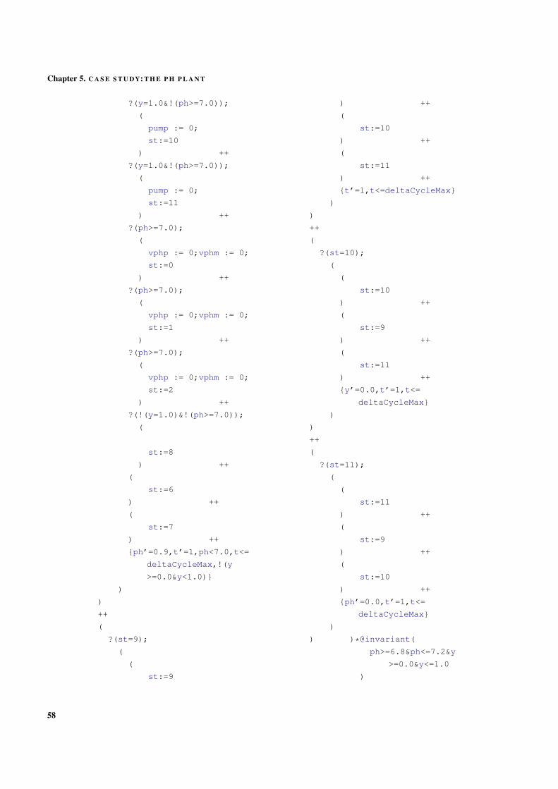
Chapter 5. C A S E S T U DY: T H E P H P L A N T
?(y=1.0&!(ph>=7.0));
(
pump := 0;
st:=10
) ++
?(y=1.0&!(ph>=7.0));
(
pump := 0;
st:=11
) ++
?(ph>=7.0);
(
vphp := 0;vphm := 0;
st:=0
) ++
?(ph>=7.0);
(
vphp := 0;vphm := 0;
st:=1
) ++
?(ph>=7.0);
(
vphp := 0;vphm := 0;
st:=2
) ++
?(!(y=1.0)&!(ph>=7.0));
(
st:=8
) ++
(
st:=6
) ++
(
st:=7
) ++
{ph’=0.9,t’=1,ph<7.0,t<=
deltaCycleMax,!(y
>=0.0&y<1.0)}
)
)
++
(
?(st=9);
(
(
st:=9
) ++
(
st:=10
) ++
(
st:=11
) ++
{t’=1,t<=deltaCycleMax}
)
)
++
(
?(st=10);
(
(
st:=10
) ++
(
st:=9
) ++
(
st:=11
) ++
{y’=0.0,t’=1,t<=
deltaCycleMax}
)
)
++
(
?(st=11);
(
(
st:=11
) ++
(
st:=9
) ++
(
st:=10
) ++
{ph’=0.0,t’=1,t<=
deltaCycleMax}
)
) )*@invariant(
ph>=6.8&ph<=7.2&y
>=0.0&y<=1.0
)
58

5.3. Verifying Safety property
\](
ph>=6.8&ph<=7.2&y>=0.0&y<=1.0
)
)
)
}
5.3 V E R I F Y I N G S A F E T Y P RO P E RT Y
The safety property to be proved by the model is that the water pH is always between 6.8 and 7.2, i.e.
0 ≤ y ≤ 1∧ 6.8 ≤ ph ≤ 7.2. The proof in KEYMAERA is shown in Figure 14.
Figure 14.: KEYMAERA window proving the safety property of the pH plant.
59

6
C O N C L U S I O N A N D F U T U R E W O R K
6.1 AC H I E V E M E N T S
PLC programs are paradigmatic in the class of safety critical software. This entails the need for
developing the methods of the verification and validation of PLC languages as proposed by the IEC
61131-3. Consequently, these languages have various formalisations. Though, most of these are
rooted in the classical techniques of verification from Computer Science, which are focusing on the
discrete dynamics of the PLC programs.
This dissertation proposed to verify PLC programs using KEYMAERA theorem prover. This lead
to the development of a tool1 based on the extension of the language SFC proposed in (Nellen and
Ábrahám, 2012), hybrid sequential function charts that also provide the translation of HSFC to hybrid
automata and on the direct representation of hybrid automata to hybrid program proposed in (Platzer,
2010). Therefore it was possible to obtain a KEYMAERA hybrid program from the each SFC programs
(detailed in Section 3.5). Consequently, this method focuses on the interaction between the discrete
and continuous dynamics of a system.
To achieve the so called hybrid sequential function charts as in the Beremiz IDE, this dissertation
proposed a series of annotations that enrich SFC programs with the conditional ordinary differential
equations and other necessary components, namely, the precondition, invariant and postcondition and
an extra annotation to trade conditions in the program, which is not translated (detailed in Section
3.3).
6.2 F U T U R E W O R K
This dissertation can be a starting point to introduce the KEYMAERA theorem prover to the industry
as a valid tool to verify and validate safety properties of PLC programs. Furthermore, several lines of
work had emerged from the work exposed in this dissertation.
• Implement the translation for the remaining languages in IEC. Evaluate IL, LD and FBD lan-
guages and find a way to translate them to KEYMAERA hybrid program.
1 Which is available at: https://github.com/Yoanribeiro/SFCToKeYmaera
61

Chapter 6. C O N C L U S I O N A N D F U T U R E W O R K
• The Structured Text language was the first language used to understand how PLC programs
work and its translation is already made to KEYMAERA. The next step is to incorporate the
annotations in the language, which entails the need for a full understanding of how the language
semantics works (the translation can be seen in Appendix A).
• Development of techniques to refine the hybrid automaton that results from HSFC translation.
In Sections 4.2.2 and 5.2.2, the resulting models are large and inelegant. This can consequently
lead to an inefficient treatment by KEYMAERA since there is a large amount of states and edges
to be considered. Furthermore, the resulting automaton can possibly be simplified to mitigate
state explosions in KEYMAERA.
• Add another annotation to enable assignment of continuous variables.
62

B I B L I O G R A P H Y
Jean-Raymond Abrial. Modeling in Event-B: System and Software Engineering. Cambridge Univer-
sity Press, New York, NY, USA, 1st edition, 2010. ISBN 0521895561, 9780521895569.
R. Alur, C. Courcoubetis, N. Halbwachs, T. A. Henzinger, P.-H. Ho, X. Nicollin, A. Olivero, J. Sifakis,
and S. Yovine. The algorithmic analysis of hybrid systems. Theoretical Computer Science, 138:
3–34, 1995.
Rajeev Alur and David L. Dill. A theory of timed automata. Theoretical Computer Science, 126:
183–235, 1994.
R. J. R. Back and F. Kurki-Suonio. Distributed cooperation with action systems. ACM Trans. Program.
Lang. Syst., 10(4):513–554, October 1988. ISSN 0164-0925. doi: 10.1145/48022.48023. URL
http://doi.acm.org/10.1145/48022.48023.
Richard Banach and Michael Butler. Cruise control in hybrid event-b. In Zhiming Liu, Jim Wood-
cock, and Huibiao Zhu, editors, Theoretical Aspects of Computing – ICTAC 2013, volume 8049 of
Lecture Notes in Computer Science, pages 76–93. Springer Berlin Heidelberg, 2013. ISBN 978-
3-642-39717-2. doi: 10.1007/978-3-642-39718-9_5. URL http://dx.doi.org/10.1007/
978-3-642-39718-9_5.
Richard Banach and Michael Butler. A hybrid event-b study of lane centering. In Marc Aigu-
ier, Frédéric Boulanger, Daniel Krob, and Clotilde Marchal, editors, Complex Systems De-
sign & Management, pages 97–111. Springer International Publishing, 2014. ISBN 978-3-
319-02811-8. doi: 10.1007/978-3-319-02812-5_8. URL http://dx.doi.org/10.1007/
978-3-319-02812-5_8.
L. Baresi, M. Mauri, A. Monti, and M. Pezze. Plctools: design, formal validation, and code gener-
ation for programmable controllers. In Systems, Man, and Cybernetics, 2000 IEEE International
Conference on, volume 4, pages 2437–2442 vol.4, 2000. doi: 10.1109/ICSMC.2000.884357.
Nanette Bauer, Ralf Huuck, Ben Lukoschus, and Sebastian Engell. A unifying semantics for sequen-
tial function charts. In Hartmut Ehrig, Werner Damm, Jörg Desel, Martin Große-Rhode, Wolfgang
Reif, Eckehard Schnieder, and Engelbert Westkämper, editors, Integration of Software Specification
Techniques for Application in Engineering, volume 3147 of Lecture Notes in Computer Science,
pages 400–418. Springer-Verlag, 2004.
63
Bibliography
Sébastien Bornot, Ralf Huuck, Ben Lukoschus, and Yassine Lakhnech. Verification of sequential func-
tion charts using smv. In In PDPTA 2000: International Conference on Parallel and Distributed
Processing Techniques and Applications, Las Vegas, pages 2987–2993, 2000a.
Sébastien Bornot, Ralf Huuck, Yassine Lakhnech, and Ben Lukoschus. Utilizing static analysis for
programmable logic controllers. In ADPM 2000 - The 4th International Conference Automation of
Mixed Processes: Hybrid Dynamic Systems, 2000b.
Ed Brinksma and Angelika Mader. Verification and optimization of a plc control schedule. In Klaus
Havelund, John Penix, and Willem Visser, editors, SPIN Model Checking and Software Verification,
volume 1885 of Lecture Notes in Computer Science, pages 73–92. Springer Berlin Heidelberg, 2000.
ISBN 978-3-540-41030-0. doi: 10.1007/10722468_5. URL http://dx.doi.org/10.1007/
10722468_5.
G. Canet, S. Couffin, J.-J. Lesage, A. Petit, and P. Schnoebelen. Towards the automatic verification of
plc programs written in instruction list. In Systems, Man, and Cybernetics, 2000 IEEE International
Conference on, volume 4, pages 2449–2454 vol.4, 2000. doi: 10.1109/ICSMC.2000.884359.
Géraud Canet. Vérification automatique des programmes écrits dans les langages de la norme IEC
61131-3. PhD thesis, 2001. URL http://www.theses.fr/2001DENS0047. Thèse de
doctorat dirigée par Petit, Antoine Informatique Cachan, Ecole normale supérieure 2001.
Zhou Chaochen, Wang Ji, and AndersP. Ravn. A formal description of hybrid systems. In Rajeev Alur,
ThomasA. Henzinger, and EduardoD. Sontag, editors, Hybrid Systems III, volume 1066 of Lecture
Notes in Computer Science, pages 511–530. Springer Berlin Heidelberg, 1996. ISBN 978-3-540-
61155-4. doi: 10.1007/BFb0020972. URL http://dx.doi.org/10.1007/BFb0020972.
Alexandre David, Dehui Du, Kim G. Larsen, Axel Legay, Marius Mikucionis, Danny Bøgsted
Poulsen, and Sean Sedwards. Statistical model checking for stochastic hybrid systems. In Ezio
Bartocci and Luca Bortolussi, editors, 1st International Workshop on Hybrid Systems and Biol-
ogy, volume 92 of Electronic Proceedings in Theoretical Computer Science, pages 122–136. Open
Publishing Association, 2012. doi: 10.4204/EPTCS.92.9.
Akash Deshpande, Aleks Göllü, and Pravin Varaiya. Shift: A formalism and a programming language
for dynamic networks of hybrid automata, 1997.
Edsger W. Dijkstra. Guarded commands, nondeterminacy and formal derivation of programs. Com-
mun. ACM, 18(8):453–457, August 1975. ISSN 0001-0782. doi: 10.1145/360933.360975. URL
http://doi.acm.org/10.1145/360933.360975.
Goran Frehse. Phaver: Algorithmic verification of hybrid systems past hytech. In Manfred Morari
and Lothar Thiele, editors, Hybrid Systems: Computation and Control, volume 3414 of Lecture
64

Bibliography
Notes in Computer Science, pages 258–273. Springer Berlin Heidelberg, 2005. ISBN 978-3-
540-25108-8. doi: 10.1007/978-3-540-31954-2_17. URL http://dx.doi.org/10.1007/
978-3-540-31954-2_17.
Carlo Ghezzi, Dino Mandrioli, Sandro Morasca, and Mauro Pezzè. A unified high-level petri net
formalism for time-critical systems. IEEE Trans. Softw. Eng., 17(2):160–172, February 1991. ISSN
0098-5589. doi: 10.1109/32.67597. URL http://dx.doi.org/10.1109/32.67597.
Roland Glück and Florian Benedikt Krebs. Towards interactive verification of programmable logic
controllers using modal kleene algebra and KIV. In Relational and Algebraic Methods in Computer
Science - 15th International Conference, RAMiCS 2015, Braga, Portugal, September 28 - October
1, 2015, Proceedings, pages 241–256, 2015. doi: 10.1007/978-3-319-24704-5_15. URL http:
//dx.doi.org/10.1007/978-3-319-24704-5_15.
David Harel, Jerzy Tiuryn, and Dexter Kozen. Dynamic Logic. MIT Press, Cambridge, MA, USA,
2000. ISBN 0262082896.
Doulgeri Z. Hassapis G., Kotini I. Validation of a sfc software specification by using hybrid automata.
In In: Proc. of INCOM 1998, pages 65—-70, 1998.
T. A. Henzinger. The theory of hybrid automata. In Proceedings of the 11th Annual IEEE Sympo-
sium on Logic in Computer Science, LICS ’96, pages 278–, Washington, DC, USA, 1996. IEEE
Computer Society. ISBN 0-8186-7463-6. URL http://dl.acm.org/citation.cfm?id=
788018.788803.
T.A. Henzinger, X. Nicollin, J. Sifakis, and S. Yovine. Symbolic model checking for real-time systems.
Information and Computation, 111(2):193 – 244, 1994. ISSN 0890-540. doi: http://dx.doi.org/
10.1006/inco.1994.1045. URL http://www.sciencedirect.com/science/article/
pii/S0890540184710455.
Thomas A. Henzinger, Pei-Hsin Ho, and Howard Wong-toi. Hytech: A model checker for hybrid
systems. Software Tools for Technology Transfer, 1:460–463, 1997.
C. A. R. Hoare. Communicating sequential processes. Commun. ACM, 21(8):666–677, August 1978.
ISSN 0001-0782. doi: 10.1145/359576.359585. URL http://doi.acm.org/10.1145/
359576.359585.
Gerard J. Holzmann. The model checker spin. IEEE Trans. Softw. Eng., 23(5):279–295, May
1997. ISSN 0098-5589. doi: 10.1109/32.588521. URL http://dx.doi.org/10.1109/
32.588521.
M Umano I Hatono, K Baba and H Tamura. Automatic generation of fault detection models for
programmable controller based manufacturing systems using complementary- places petri nets. In
13th IFAC Congress, 1996.
65

Bibliography
Jean-Baptiste Jeannin, Khalil Ghorbal, Yanni Kouskoulas, Ryan Gardner, Aurora Schmidt, and Erik
Zawadzki André Platzer. A formally verified hybrid system for the next-generation airborne col-
lision avoidance system. In Christel Baier and Cesare Tinelli, editors, TACAS, LNCS. Springer,
2015.
Karl Heinz John and Michael Tiegelkamp. IEC 61131-3: Programming Industrial Automation Sys-
tems. Springer, 2nd edition, 2010. ISBN 3642120148, 9783642120145.
S. Kowalewski, N. Bauer, J. Preussig, O. Stursberg, and H. Treseler. An environment for model-
checking of logic control systems with hybrid dynamics. In Computer Aided Control System Design,
1999. Proceedings of the 1999 IEEE International Symposium on, pages 97–102, 1999. doi: 10.
1109/CACSD.1999.808631.
Stefan Kowalewski, Sebastian Engell, Ralf Huuck, Yassine Lakhnech, Ben Lukoschus, and Luis
Urbina. Using model-checking for timed automata to parameterize logic control programs. In
In Proc. of the 8th European Symp. on Computer Computer Aided Process Engineering (ESCAPE,
pages 24–27, 1998.
Kim G. Larsen, Paul Pettersson, and Wang Yi. Model-Checking for Real-Time Systems. In Proc. of
Fundamentals of Computation Theory, number 965 in Lecture Notes in Computer Science, pages
62–88, August 1995.
Jiang Liu, Jidong Lv, Zhao Quan, Naijun Zhan, Hengjun Zhao, Chaochen Zhou, and Liang Zou. A
calculus for hybrid csp. In Kazunori Ueda, editor, Programming Languages and Systems, vol-
ume 6461 of Lecture Notes in Computer Science, pages 1–15. Springer Berlin Heidelberg, 2010.
ISBN 978-3-642-17163-5. doi: 10.1007/978-3-642-17164-2_1. URL http://dx.doi.org/
10.1007/978-3-642-17164-2_1.
Sarah M. Loos and André Platzer. Safe intersections: At the crossing of hybrid systems and verifica-
tion. In Kyongsu Yi, editor, ITSC, pages 1181–1186, 2011. doi: 10.1109/ITSC.2011.6083138.
Sarah M. Loos, André Platzer, and Ligia Nistor. Adaptive cruise control: Hybrid, distributed, and
now formally verified. In Michael Butler and Wolfram Schulte, editors, FM, volume 6664 of LNCS,
pages 42–56. Springer, 2011. doi: 10.1007/978-3-642-21437-0_6.
Nancy Lynch, Roberto Segala, and Frits Vaandrager. Hybrid i/o automata. Informa-
tion and Computation, 185(1):105–157, 2003. ISSN 0890-5401. doi: http://dx.doi.org/
10.1016/S0890-5401(03)00067-1. URL http://www.sciencedirect.com/science/
article/pii/S0890540103000671.
A. Mader and H. Wupper. Timed automaton models for simple programmable logic controllers. In
Real-Time Systems, 1999. Proceedings of the 11th Euromicro Conference on, pages 106–113, 1999.
doi: 10.1109/EMRTS.1999.777456.
66
Bibliography
A.H. Mader, H. Brinksma, H. Wupper, and N. Bauer. Design of a plc control program for a batch
plant - vhs case study 1. European Journal of Control, 7(4):416–439, 2001. URL http://doc.
utwente.nl/66969/. Imported from DIES.
K. L. Mcmillan. The smv system, 1992.
T. Mertke and Thomas Menzel. Methods and tools to the verification of safety-related control software.
In Systems, Man, and Cybernetics, 2000 IEEE International Conference on, volume 4, pages 2455–
2457 vol.4, 2000. doi: 10.1109/ICSMC.2000.884360.
Johanna Nellen and Erika Ábrahám. Hybrid sequential function charts. In Jens Brandt and
Klaus Schneider 0001, editors, MBMV, pages 109–120. Verlag Dr. Kovac, 2012. URL http:
//dblp.uni-trier.de/db/conf/mbmv/mbmv2012.html#NellenA12.
André Platzer. Logical Analysis of Hybrid Systems:Proving Theorems for Complex Dynamics.
Springer, Heidelberg, 2010. ISBN 978-3-642-14508-7. doi: 10.1007/978-3-642-14509-4.
André Platzer and Edmund M. Clarke. Formal verification of curved flight collision avoidance ma-
neuvers: A case study. In Ana Cavalcanti and Dennis Dams, editors, FM, volume 5850 of LNCS,
pages 547–562. Springer, 2009. doi: 10.1007/978-3-642-05089-3_35.
André Platzer and Jan-David Quesel. European Train Control System: A case study in formal ver-
ification. In Karin Breitman and Ana Cavalcanti, editors, ICFEM, volume 5885 of LNCS, pages
246–265. Springer, 2009. doi: 10.1007/978-3-642-10373-5_13.
Wolfgang Reif. The kiv system: Systematic construction of verified software. In Deepak Kapur, editor,
Automated Deduction—CADE-11, volume 607 of Lecture Notes in Computer Science, pages 753–
757. Springer Berlin Heidelberg, 1992. ISBN 978-3-540-55602-2. doi: 10.1007/3-540-55602-8_
218. URL http://dx.doi.org/10.1007/3-540-55602-8_218.
Mauno Rönkkö, Anders P. Ravn, and Kaisa Sere. Hybrid action systems. Theoreti-
cal Computer Science, 290(1):937–973, 2003. ISSN 0304-3975. doi: http://dx.doi.org/
10.1016/S0304-3975(02)00547-9. URL http://www.sciencedirect.com/science/
article/pii/S0304397502005479.
Mauno Rönkkö and Xuandong Li. Linear hybrid action systems. Nordic J. of Computing, 8(1):
159–177, March 2001. ISSN 1236-6064. URL http://dl.acm.org/citation.cfm?id=
774194.774202.
O. Rossi and Ph. Schnoebelen. Formal modeling of timed function blocks for the automatic verifica-
tion of ladder diagram programs, 2000.
Jean-Marc Roussel and Jean-Jacques Lesage. Validation and verification of grafcets using state
machine. In IMACS-IEEE ”CESA’96”, pages pp. 758–764, Lille, France, July 1996. URL
https://hal.archives-ouvertes.fr/hal-00353188.
67
Bibliography
R.S. Sreenivas and B.H. Krogh. On condition/event systems with discrete state realizations. Discrete
Event Dynamic Systems, 1(2):209–236, 1991. ISSN 0924-6703. doi: 10.1007/BF01805563. URL
http://dx.doi.org/10.1007/BF01805563.
E. Tisserant, L. Bessard, and M. de Sousa. An open source iec 61131-3 integrated development
environment. In Industrial Informatics, 2007 5th IEEE International Conference on, volume 1,
pages 183–187, June 2007. doi: 10.1109/INDIN.2007.4384753.
H.X. Willems. Compact timed automata for plc programs, 1999.
M. Bani Younis and G. Frey. Formalization of existing PLC programs: A survey. In Proceedings of
Computing Engineering in Systems Applications, Lille, France, 2003.
68

AAU X I L A RY W O R K : S T T O K E Y M A E R A
Keyword Description Example KeYmaera:= Assignment d := 10; d := 10.
Call of an FBFBName();
Replacement of the call
by its respective code as-
signing the input variables
with the right values
IF Selection
IF b THEN a
ELSIF d
THEN c
ELSE d
END_IF(?b);(a)
++
(?~b && d);c
++
(?~b && ~d);d
69
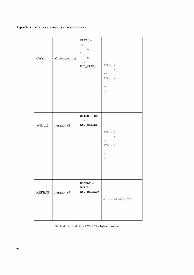
Appendix A. AU X I L A R Y W O R K : S T T O K E Y M A E R A
CASE Multi-selection
CASE(b)
1:
a
2:
b
...
END_CASE; (?b=1);
a
++
(?b=2);
b
++
...
WHILE Iteration (2)
WHILE n DO
a
END_WHILE;
(?b=1);
a
++
(?b=2);
b
++
...
REPEAT Iteration (3)
REPEAT a
UNTIL b
END_REPEAT;
a;((?~b);a)*;(?b)
Table 4.: ST code to KEYMAERA hybrid program
70
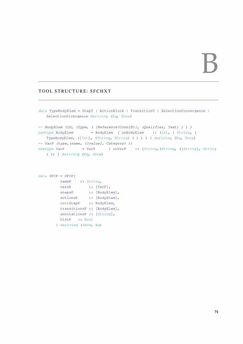
BT O O L S T RU C T U R E : S F C H X T
data TypeBodyElem = StepT | ActionBlock | TransitionT | SelectionConvergence |
SelectionDivergence deriving (Eq, Show)
-- BodyElem (ID, (Type, ( [Reference(ConnIN)], (Qualifier, Text) ) ) )
newtype BodyElem = BodyElem { unBodyElem :: (Int, ( String, (
TypeBodyElem, ([Int], (String, String) ) ) ) ) } deriving (Eq, Show)
-- VarP (type,(name, ([value], Category) ))
newtype VarP = VarP { unVarP :: (String,(String, ([String], String
) )) } deriving (Eq, Show)
data SFCP = SFCP{
nameP :: String,
varsP :: [VarP],
stepsP :: [BodyElem],
actionsP :: [BodyElem],
initStepP :: BodyElem,
transitionsP :: [BodyElem],
annotationsP :: [String],
histP :: Bool
} deriving (Show, Eq)
71

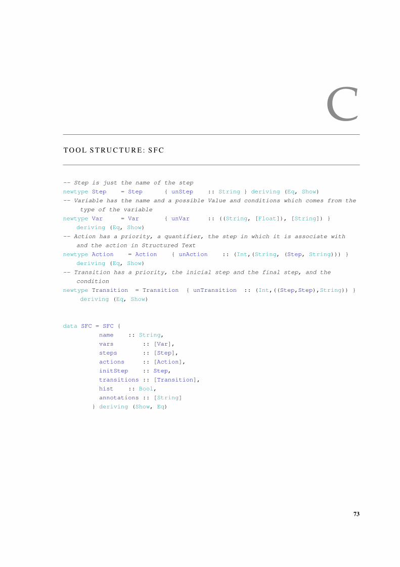
CT O O L S T RU C T U R E : S F C
-- Step is just the name of the step
newtype Step = Step { unStep :: String } deriving (Eq, Show)
-- Variable has the name and a possible Value and conditions which comes from the
type of the variable
newtype Var = Var { unVar :: ((String, [Float]), [String]) }
deriving (Eq, Show)
-- Action has a priority, a quantifier, the step in which it is associate with
and the action in Structured Text
newtype Action = Action { unAction :: (Int,(String, (Step, String))) }
deriving (Eq, Show)
-- Transition has a priority, the inicial step and the final step, and the
condition
newtype Transition = Transition { unTransition :: (Int,((Step,Step),String)) }
deriving (Eq, Show)
data SFC = SFC {
name :: String,
vars :: [Var],
steps :: [Step],
actions :: [Action],
initStep :: Step,
transitions :: [Transition],
hist :: Bool,
annotations :: [String]
} deriving (Show, Eq)
73


DT O O L S T RU C T U R E : H Y B R I D AU T O M AT O N
-- VarH represents a variable of the HA which can have a inicial value,
represented as a singleton list of Float, and it also has another singleton
list which represents extra condition about the variable
newtype VarH = VarH { unVarH :: ((String, [Float]), [String]) }
deriving (Eq, Show, Ord)
-- Loc is a Node of the HA
newtype Loc = Loc { unLoc :: String } deriving (Eq, Show)
-- Edge is self-explanatory ((source,target),(condition,assignments))
newtype Edge = Edge { unEdge :: ((Loc,Loc), (String, String)) } deriving (Eq,
Show)
-- Invariant of a Loc
newtype Inv = Inv { unInv :: (Loc,String) } deriving (Eq, Show)
-- Differential Equation for a Loc
newtype Flow = Flow { unFlow :: (Loc,String) } deriving (Eq, Show)
-- Map between [Loc] and [Int]
data HybridAutomaton = HA {
nameH :: String,
varsH :: [VarH],
locs :: [Loc],
edges :: [Edge],
invs :: [Inv],
flows :: [Flow],
initH :: Loc,
initCond :: String,
toProve :: String,
cycleInv :: String
} deriving (Show, Eq)
75


EC A S E S T U DY: WAT E R H E AT I N G TA N K X M L
<pou name="WatertankCtrl" pouType="functionBlock">
<interface>
<localVars>
<variable name="pump">
<type>
<BOOL/>
</type>
</variable>
<variable name="dv">
<type>
<BOOL/>
</type>
</variable>
</localVars>
<inputVars>
<variable name="Start">
<type>
<BOOL/>
</type>
</variable>
</inputVars>
<outputVars>
<variable name="heater">
<type>
<BOOL/>
</type>
</variable>
<variable name="Full">
<type>
<BOOL/>
</type>
</variable>
<variable name="Empty">
<type>
<BOOL/>
77

Appendix E. C A S E S T U DY: WAT E R H E AT I N G TA N K X M L
</type>
</variable>
</outputVars>
<localVars>
<variable name="tm">
<type>
<INT/>
</type>
</variable>
</localVars>
<outputVars>
<variable name="temp">
<type>
<INT/>
</type>
</variable>
</outputVars>
</interface>
<body>
<SFC>
<step localId="1" name="Step0" initialStep="true" height="27" width="
42">
<position x="348" y="31"/>
<connectionPointIn>
<relPosition x="21" y="0"/>
<connection refLocalId="10">
<position x="369" y="31"/>
<position x="369" y="21"/>
<position x="299" y="21"/>
<position x="299" y="380"/>
<position x="370" y="380"/>
<position x="370" y="370"/>
</connection>
</connectionPointIn>
<connectionPointOut formalParameter="">
<relPosition x="21" y="27"/>
</connectionPointOut>
</step>
<step localId="2" name="Step1" initialStep="false" height="23" width=
"38">
<position x="350" y="109"/>
<connectionPointIn>
<relPosition x="19" y="0"/>
<connection refLocalId="6">
<position x="369" y="109"/>
<position x="369" y="84"/>
</connection>
78
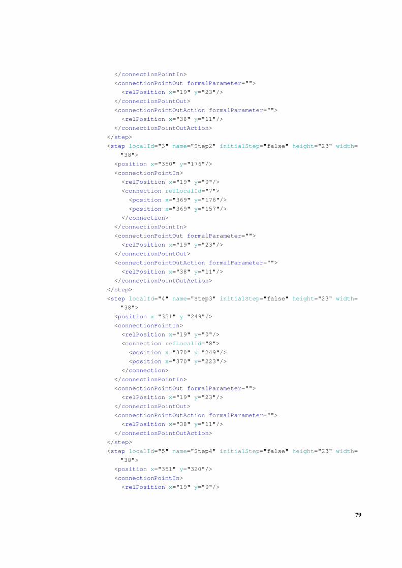
</connectionPointIn>
<connectionPointOut formalParameter="">
<relPosition x="19" y="23"/>
</connectionPointOut>
<connectionPointOutAction formalParameter="">
<relPosition x="38" y="11"/>
</connectionPointOutAction>
</step>
<step localId="3" name="Step2" initialStep="false" height="23" width=
"38">
<position x="350" y="176"/>
<connectionPointIn>
<relPosition x="19" y="0"/>
<connection refLocalId="7">
<position x="369" y="176"/>
<position x="369" y="157"/>
</connection>
</connectionPointIn>
<connectionPointOut formalParameter="">
<relPosition x="19" y="23"/>
</connectionPointOut>
<connectionPointOutAction formalParameter="">
<relPosition x="38" y="11"/>
</connectionPointOutAction>
</step>
<step localId="4" name="Step3" initialStep="false" height="23" width=
"38">
<position x="351" y="249"/>
<connectionPointIn>
<relPosition x="19" y="0"/>
<connection refLocalId="8">
<position x="370" y="249"/>
<position x="370" y="223"/>
</connection>
</connectionPointIn>
<connectionPointOut formalParameter="">
<relPosition x="19" y="23"/>
</connectionPointOut>
<connectionPointOutAction formalParameter="">
<relPosition x="38" y="11"/>
</connectionPointOutAction>
</step>
<step localId="5" name="Step4" initialStep="false" height="23" width=
"38">
<position x="351" y="320"/>
<connectionPointIn>
<relPosition x="19" y="0"/>
79

Appendix E. C A S E S T U DY: WAT E R H E AT I N G TA N K X M L
<connection refLocalId="9">
<position x="370" y="320"/>
<position x="370" y="299"/>
</connection>
</connectionPointIn>
<connectionPointOut formalParameter="">
<relPosition x="19" y="23"/>
</connectionPointOut>
<connectionPointOutAction formalParameter="">
<relPosition x="38" y="11"/>
</connectionPointOutAction>
</step>
<transition localId="6" height="2" width="20">
<position x="359" y="82"/>
<connectionPointIn>
<relPosition x="10" y="0"/>
<connection refLocalId="1">
<position x="369" y="82"/>
<position x="369" y="58"/>
</connection>
</connectionPointIn>
<connectionPointOut>
<relPosition x="10" y="2"/>
</connectionPointOut>
<condition>
<inline name="">
<ST>
<xhtml:p><![CDATA[Empty = TRUE & Start = TRUE]]></xhtml:p>
</ST>
</inline>
</condition>
</transition>
<transition localId="7" height="2" width="20">
<position x="359" y="155"/>
<connectionPointIn>
<relPosition x="10" y="0"/>
<connection refLocalId="2">
<position x="369" y="155"/>
<position x="369" y="132"/>
</connection>
</connectionPointIn>
<connectionPointOut>
<relPosition x="10" y="2"/>
</connectionPointOut>
<condition>
<inline name="">
<ST>
80

<xhtml:p><![CDATA[Full = TRUE]]></xhtml:p>
</ST>
</inline>
</condition>
</transition>
<transition localId="8" height="2" width="20">
<position x="360" y="221"/>
<connectionPointIn>
<relPosition x="10" y="0"/>
<connection refLocalId="3">
<position x="370" y="221"/>
<position x="370" y="210"/>
<position x="369" y="210"/>
<position x="369" y="199"/>
</connection>
</connectionPointIn>
<connectionPointOut>
<relPosition x="10" y="2"/>
</connectionPointOut>
<condition>
<inline name="">
<ST>
<xhtml:p><![CDATA[temp = 90]]></xhtml:p>
</ST>
</inline>
</condition>
</transition>
<transition localId="9" height="2" width="20">
<position x="360" y="297"/>
<connectionPointIn>
<relPosition x="10" y="0"/>
<connection refLocalId="4">
<position x="370" y="297"/>
<position x="370" y="272"/>
</connection>
</connectionPointIn>
<connectionPointOut>
<relPosition x="10" y="2"/>
</connectionPointOut>
<condition>
<inline name="">
<ST>
<xhtml:p><![CDATA[tm = 20]]></xhtml:p>
</ST>
</inline>
</condition>
</transition>
81
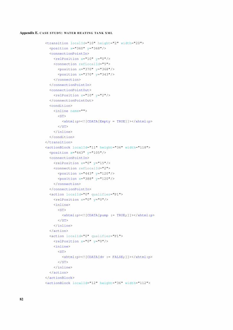
Appendix E. C A S E S T U DY: WAT E R H E AT I N G TA N K X M L
<transition localId="10" height="2" width="20">
<position x="360" y="368"/>
<connectionPointIn>
<relPosition x="10" y="0"/>
<connection refLocalId="5">
<position x="370" y="368"/>
<position x="370" y="343"/>
</connection>
</connectionPointIn>
<connectionPointOut>
<relPosition x="10" y="2"/>
</connectionPointOut>
<condition>
<inline name="">
<ST>
<xhtml:p><![CDATA[Empty = TRUE]]></xhtml:p>
</ST>
</inline>
</condition>
</transition>
<actionBlock localId="11" height="36" width="118">
<position x="443" y="105"/>
<connectionPointIn>
<relPosition x="0" y="15"/>
<connection refLocalId="2">
<position x="443" y="120"/>
<position x="388" y="120"/>
</connection>
</connectionPointIn>
<action localId="0" qualifier="P1">
<relPosition x="0" y="0"/>
<inline>
<ST>
<xhtml:p><![CDATA[pump := TRUE;]]></xhtml:p>
</ST>
</inline>
</action>
<action localId="0" qualifier="P1">
<relPosition x="0" y="0"/>
<inline>
<ST>
<xhtml:p><![CDATA[dv := FALSE;]]></xhtml:p>
</ST>
</inline>
</action>
</actionBlock>
<actionBlock localId="12" height="36" width="112">
82

<position x="468" y="172"/>
<connectionPointIn>
<relPosition x="0" y="15"/>
<connection refLocalId="3">
<position x="468" y="187"/>
<position x="388" y="187"/>
</connection>
</connectionPointIn>
<action localId="0" qualifier="P1">
<relPosition x="0" y="0"/>
<inline>
<ST>
<xhtml:p><![CDATA[pump := FALSE;]]></xhtml:p>
</ST>
</inline>
</action>
<action localId="0" qualifier="P1">
<relPosition x="0" y="0"/>
<inline>
<ST>
<xhtml:p><![CDATA[heater := TRUE;]]></xhtml:p>
</ST>
</inline>
</action>
</actionBlock>
<actionBlock localId="13" height="36" width="116">
<position x="463" y="245"/>
<connectionPointIn>
<relPosition x="0" y="15"/>
<connection refLocalId="4">
<position x="463" y="260"/>
<position x="389" y="260"/>
</connection>
</connectionPointIn>
<action localId="0" qualifier="P1">
<relPosition x="0" y="0"/>
<inline>
<ST>
<xhtml:p><![CDATA[heater := FALSE;]]></xhtml:p>
</ST>
</inline>
</action>
<action localId="0" qualifier="P1">
<relPosition x="0" y="0"/>
<inline>
<ST>
<xhtml:p><![CDATA[tm := 0;]]></xhtml:p>
83
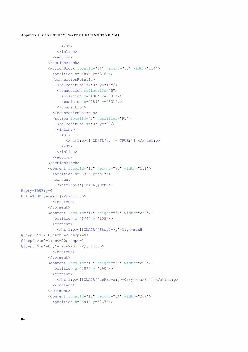
Appendix E. C A S E S T U DY: WAT E R H E AT I N G TA N K X M L
</ST>
</inline>
</action>
</actionBlock>
<actionBlock localId="14" height="30" width="114">
<position x="480" y="316"/>
<connectionPointIn>
<relPosition x="0" y="15"/>
<connection refLocalId="5">
<position x="480" y="331"/>
<position x="389" y="331"/>
</connection>
</connectionPointIn>
<action localId="0" qualifier="P1">
<relPosition x="0" y="0"/>
<inline>
<ST>
<xhtml:p><![CDATA[dv := TRUE;]]></xhtml:p>
</ST>
</inline>
</action>
</actionBlock>
<comment localId="15" height="70" width="151">
<position x="636" y="51"/>
<content>
<xhtml:p><![CDATA[@Extra:
Empty=TRUE:y=0
Full=TRUE:y=maxH]]></xhtml:p>
</content>
</comment>
<comment localId="16" height="36" width="264">
<position x="670" y="153"/>
<content>
<xhtml:p><![CDATA[@Step2->y’=1:y<=maxH
@Step3->y’= 0;temp’=2:temp<=90
@Step4->tm’=1:tm<=20;temp’=0
@Step5->tm’=0;y’=-2:y>=0]]></xhtml:p>
</content>
</comment>
<comment localId="17" height="36" width="200">
<position x="707" y="300"/>
<content>
<xhtml:p><![CDATA[@toProve:y>=0&&y<=maxH ]]></xhtml:p>
</content>
</comment>
<comment localId="18" height="36" width="207">
<position x="694" y="237"/>
84

<content>
<xhtml:p><![CDATA[@invariant:h>=0&&h<=maxH]]></xhtml:p>
</content>
</comment>
<comment localId="19" height="36" width="275">
<position x="699" y="209"/>
<content>
<xhtml:p><![CDATA[@initCond:maxH>0&&y>=0&&y<=maxH]]></xhtml:p>
</content>
</comment>
</SFC>
</body>
</pou>
85

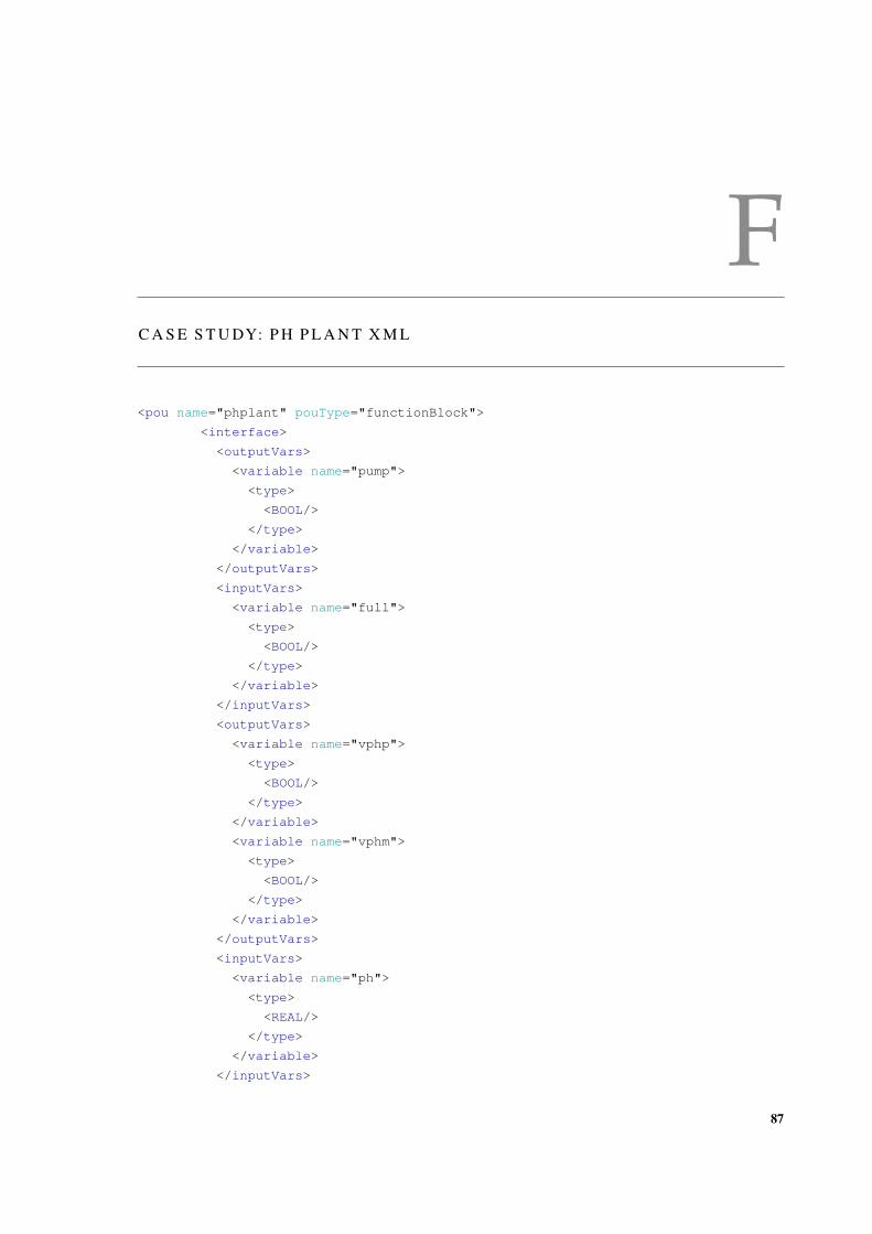
FC A S E S T U DY: P H P L A N T X M L
<pou name="phplant" pouType="functionBlock">
<interface>
<outputVars>
<variable name="pump">
<type>
<BOOL/>
</type>
</variable>
</outputVars>
<inputVars>
<variable name="full">
<type>
<BOOL/>
</type>
</variable>
</inputVars>
<outputVars>
<variable name="vphp">
<type>
<BOOL/>
</type>
</variable>
<variable name="vphm">
<type>
<BOOL/>
</type>
</variable>
</outputVars>
<inputVars>
<variable name="ph">
<type>
<REAL/>
</type>
</variable>
</inputVars>
87
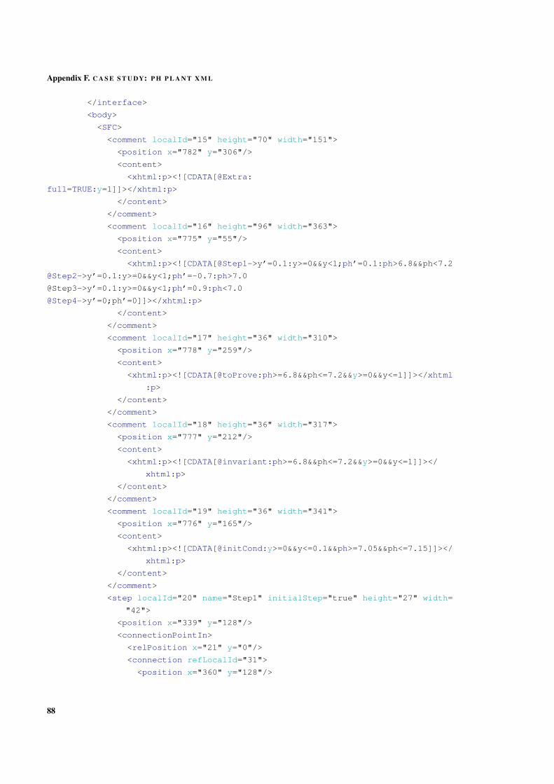
Appendix F. C A S E S T U DY: P H P L A N T X M L
</interface>
<body>
<SFC>
<comment localId="15" height="70" width="151">
<position x="782" y="306"/>
<content>
<xhtml:p><![CDATA[@Extra:
full=TRUE:y=1]]></xhtml:p>
</content>
</comment>
<comment localId="16" height="96" width="363">
<position x="775" y="55"/>
<content>
<xhtml:p><![CDATA[@Step1->y’=0.1:y>=0&&y<1;ph’=0.1:ph>6.8&&ph<7.2
@Step2->y’=0.1:y>=0&&y<1;ph’=-0.7:ph>7.0
@Step3->y’=0.1:y>=0&&y<1;ph’=0.9:ph<7.0
@Step4->y’=0;ph’=0]]></xhtml:p>
</content>
</comment>
<comment localId="17" height="36" width="310">
<position x="778" y="259"/>
<content>
<xhtml:p><![CDATA[@toProve:ph>=6.8&&ph<=7.2&&y>=0&&y<=1]]></xhtml
:p>
</content>
</comment>
<comment localId="18" height="36" width="317">
<position x="777" y="212"/>
<content>
<xhtml:p><![CDATA[@invariant:ph>=6.8&&ph<=7.2&&y>=0&&y<=1]]></
xhtml:p>
</content>
</comment>
<comment localId="19" height="36" width="341">
<position x="776" y="165"/>
<content>
<xhtml:p><![CDATA[@initCond:y>=0&&y<=0.1&&ph>=7.05&&ph<=7.15]]></
xhtml:p>
</content>
</comment>
<step localId="20" name="Step1" initialStep="true" height="27" width=
"42">
<position x="339" y="128"/>
<connectionPointIn>
<relPosition x="21" y="0"/>
<connection refLocalId="31">
<position x="360" y="128"/>
88
<position x="360" y="117"/>
<position x="360" y="117"/>
<position x="360" y="105"/>
</connection>
</connectionPointIn>
<connectionPointOut formalParameter="">
<relPosition x="21" y="27"/>
</connectionPointOut>
<connectionPointOutAction formalParameter="">
<relPosition x="42" y="13"/>
</connectionPointOutAction>
</step>
<actionBlock localId="21" height="36" width="110">
<position x="400" y="126"/>
<connectionPointIn>
<relPosition x="0" y="15"/>
<connection refLocalId="20">
<position x="400" y="141"/>
<position x="381" y="141"/>
</connection>
</connectionPointIn>
<action localId="0" qualifier="P1">
<relPosition x="0" y="0"/>
<inline>
<ST>
<xhtml:p><![CDATA[vphp := FALSE;]]></xhtml:p>
</ST>
</inline>
</action>
<action localId="0" qualifier="P1">
<relPosition x="0" y="0"/>
<inline>
<ST>
<xhtml:p><![CDATA[vphm := FALSE;]]></xhtml:p>
</ST>
</inline>
</action>
</actionBlock>
<selectionDivergence localId="22" height="1" width="282">
<position x="218" y="175"/>
<connectionPointIn>
<relPosition x="142" y="0"/>
<connection refLocalId="20">
<position x="360" y="175"/>
<position x="360" y="157"/>
<position x="360" y="157"/>
<position x="360" y="165"/>
89

Appendix F. C A S E S T U DY: P H P L A N T X M L
<position x="360" y="165"/>
<position x="360" y="155"/>
</connection>
</connectionPointIn>
<connectionPointOut formalParameter="">
<relPosition x="0" y="1"/>
</connectionPointOut>
<connectionPointOut formalParameter="">
<relPosition x="142" y="1"/>
</connectionPointOut>
<connectionPointOut formalParameter="">
<relPosition x="282" y="1"/>
</connectionPointOut>
</selectionDivergence>
<step localId="23" name="Step2" initialStep="false" height="23" width
="38">
<position x="199" y="222"/>
<connectionPointIn>
<relPosition x="19" y="0"/>
<connection refLocalId="24">
<position x="218" y="222"/>
<position x="218" y="196"/>
</connection>
</connectionPointIn>
<connectionPointOut formalParameter="">
<relPosition x="19" y="23"/>
</connectionPointOut>
<connectionPointOutAction formalParameter="">
<relPosition x="38" y="11"/>
</connectionPointOutAction>
</step>
<transition localId="24" height="2" width="20">
<position x="208" y="194"/>
<connectionPointIn>
<relPosition x="10" y="0"/>
<connection refLocalId="22">
<position x="218" y="194"/>
<position x="218" y="184"/>
<position x="218" y="184"/>
<position x="218" y="176"/>
</connection>
</connectionPointIn>
<connectionPointOut>
<relPosition x="10" y="2"/>
</connectionPointOut>
<condition>
<inline name="">
90
<ST>
<xhtml:p><![CDATA[ph >= 7.2]]></xhtml:p>
</ST>
</inline>
</condition>
</transition>
<step localId="25" name="Step3" initialStep="false" height="23" width
="38">
<position x="481" y="221"/>
<connectionPointIn>
<relPosition x="19" y="0"/>
<connection refLocalId="26">
<position x="500" y="221"/>
<position x="500" y="211"/>
<position x="500" y="211"/>
<position x="500" y="196"/>
</connection>
</connectionPointIn>
<connectionPointOut formalParameter="">
<relPosition x="19" y="23"/>
</connectionPointOut>
<connectionPointOutAction formalParameter="">
<relPosition x="38" y="11"/>
</connectionPointOutAction>
</step>
<transition localId="26" height="2" width="20">
<position x="490" y="194"/>
<connectionPointIn>
<relPosition x="10" y="0"/>
<connection refLocalId="22">
<position x="500" y="194"/>
<position x="500" y="184"/>
<position x="500" y="184"/>
<position x="500" y="176"/>
</connection>
</connectionPointIn>
<connectionPointOut>
<relPosition x="10" y="2"/>
</connectionPointOut>
<condition>
<inline name="">
<ST>
<xhtml:p><![CDATA[ph <= 6.8]]></xhtml:p>
</ST>
</inline>
</condition>
</transition>
91
Appendix F. C A S E S T U DY: P H P L A N T X M L
<step localId="27" name="Step4" initialStep="false" height="23" width
="38">
<position x="341" y="394"/>
<connectionPointIn>
<relPosition x="19" y="0"/>
<connection refLocalId="28">
<position x="360" y="394"/>
<position x="360" y="370"/>
</connection>
</connectionPointIn>
<connectionPointOutAction formalParameter="">
<relPosition x="38" y="11"/>
</connectionPointOutAction>
</step>
<selectionConvergence localId="28" height="1" width="175">
<position x="272" y="369"/>
<connectionPointIn>
<relPosition x="0" y="0"/>
<connection refLocalId="32">
<position x="272" y="369"/>
<position x="272" y="345"/>
</connection>
</connectionPointIn>
<connectionPointIn>
<relPosition x="88" y="0"/>
<connection refLocalId="33">
<position x="360" y="369"/>
<position x="360" y="303"/>
</connection>
</connectionPointIn>
<connectionPointIn>
<relPosition x="175" y="0"/>
<connection refLocalId="1">
<position x="447" y="369"/>
<position x="447" y="342"/>
</connection>
</connectionPointIn>
<connectionPointOut>
<relPosition x="88" y="1"/>
</connectionPointOut>
</selectionConvergence>
<selectionDivergence localId="29" height="1" width="110">
<position x="162" y="280"/>
<connectionPointIn>
<relPosition x="56" y="0"/>
<connection refLocalId="23">
<position x="218" y="280"/>
92

<position x="218" y="270"/>
<position x="218" y="270"/>
<position x="218" y="245"/>
</connection>
</connectionPointIn>
<connectionPointOut formalParameter="">
<relPosition x="0" y="1"/>
</connectionPointOut>
<connectionPointOut formalParameter="">
<relPosition x="110" y="1"/>
</connectionPointOut>
</selectionDivergence>
<selectionDivergence localId="30" height="1" width="106">
<position x="447" y="268"/>
<connectionPointIn>
<relPosition x="53" y="0"/>
<connection refLocalId="25">
<position x="500" y="268"/>
<position x="500" y="250"/>
<position x="500" y="250"/>
<position x="500" y="260"/>
</connection>
</connectionPointIn>
<connectionPointOut formalParameter="">
<relPosition x="0" y="1"/>
</connectionPointOut>
<connectionPointOut formalParameter="">
<relPosition x="106" y="1"/>
</connectionPointOut>
</selectionDivergence>
<selectionConvergence localId="31" height="1" width="40">
<position x="340" y="104"/>
<connectionPointIn>
<relPosition x="0" y="0"/>
<connection refLocalId="35">
<position x="340" y="104"/>
<position x="340" y="86"/>
<position x="131" y="86"/>
<position x="131" y="237"/>
<position x="131" y="237"/>
<position x="131" y="178"/>
</connection>
</connectionPointIn>
<connectionPointIn>
<relPosition x="40" y="0"/>
<connection refLocalId="36">
<position x="380" y="104"/>
93
Appendix F. C A S E S T U DY: P H P L A N T X M L
<position x="380" y="86"/>
<position x="683" y="86"/>
<position x="683" y="302"/>
<position x="683" y="302"/>
<position x="683" y="167"/>
</connection>
</connectionPointIn>
<connectionPointOut>
<relPosition x="20" y="1"/>
</connectionPointOut>
</selectionConvergence>
<transition localId="32" height="13" width="20">
<position x="262" y="332"/>
<connectionPointIn>
<relPosition x="10" y="0"/>
<connection refLocalId="29">
<position x="272" y="332"/>
<position x="272" y="281"/>
</connection>
</connectionPointIn>
<connectionPointOut>
<relPosition x="10" y="13"/>
</connectionPointOut>
<condition>
<inline name="">
<ST>
<xhtml:p><![CDATA[full = TRUE]]></xhtml:p>
</ST>
</inline>
</condition>
</transition>
<transition localId="1" height="3" width="20" executionOrderId="0">
<position x="437" y="339"/>
<connectionPointIn>
<relPosition x="10" y="0"/>
<connection refLocalId="30">
<position x="447" y="339"/>
<position x="447" y="269"/>
</connection>
</connectionPointIn>
<connectionPointOut>
<relPosition x="10" y="3"/>
</connectionPointOut>
<condition>
<inline name="">
<ST>
<xhtml:p><![CDATA[full = TRUE]]></xhtml:p>
94
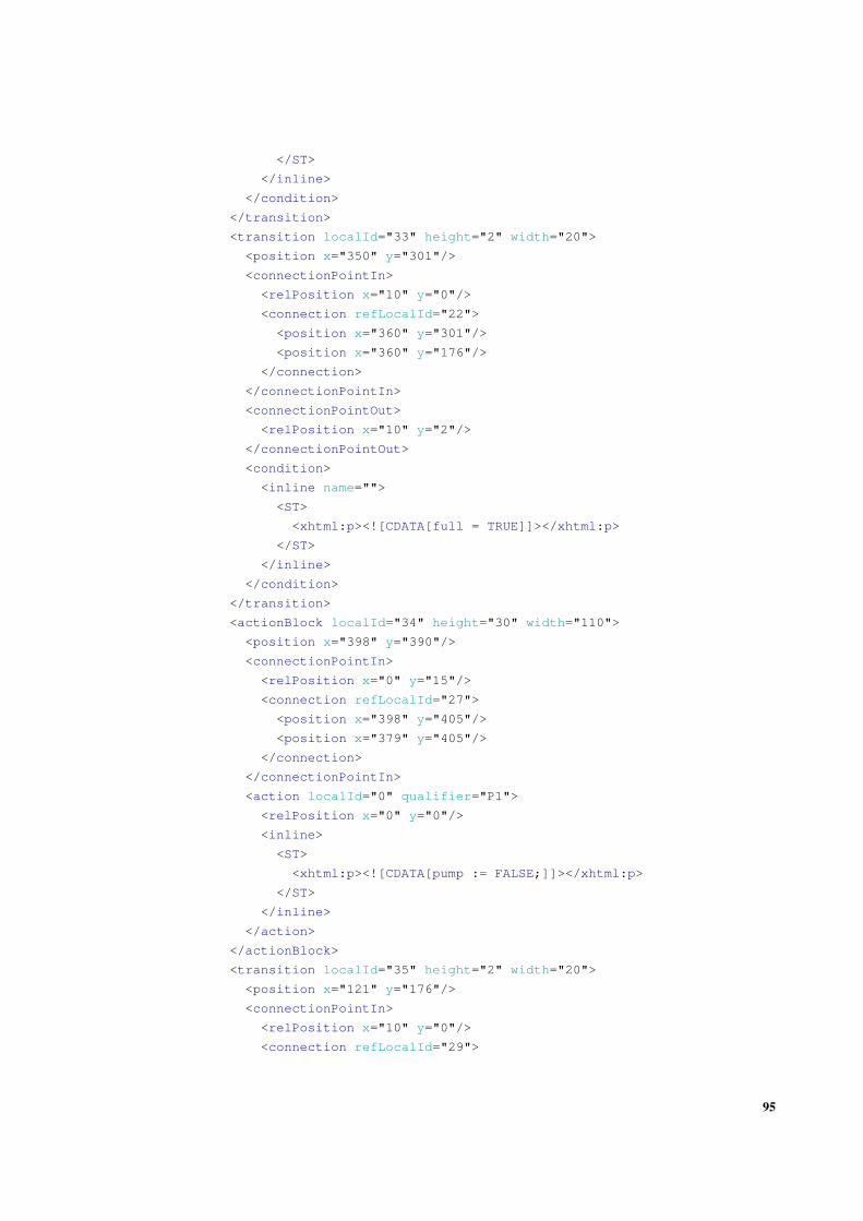
</ST>
</inline>
</condition>
</transition>
<transition localId="33" height="2" width="20">
<position x="350" y="301"/>
<connectionPointIn>
<relPosition x="10" y="0"/>
<connection refLocalId="22">
<position x="360" y="301"/>
<position x="360" y="176"/>
</connection>
</connectionPointIn>
<connectionPointOut>
<relPosition x="10" y="2"/>
</connectionPointOut>
<condition>
<inline name="">
<ST>
<xhtml:p><![CDATA[full = TRUE]]></xhtml:p>
</ST>
</inline>
</condition>
</transition>
<actionBlock localId="34" height="30" width="110">
<position x="398" y="390"/>
<connectionPointIn>
<relPosition x="0" y="15"/>
<connection refLocalId="27">
<position x="398" y="405"/>
<position x="379" y="405"/>
</connection>
</connectionPointIn>
<action localId="0" qualifier="P1">
<relPosition x="0" y="0"/>
<inline>
<ST>
<xhtml:p><![CDATA[pump := FALSE;]]></xhtml:p>
</ST>
</inline>
</action>
</actionBlock>
<transition localId="35" height="2" width="20">
<position x="121" y="176"/>
<connectionPointIn>
<relPosition x="10" y="0"/>
<connection refLocalId="29">
95
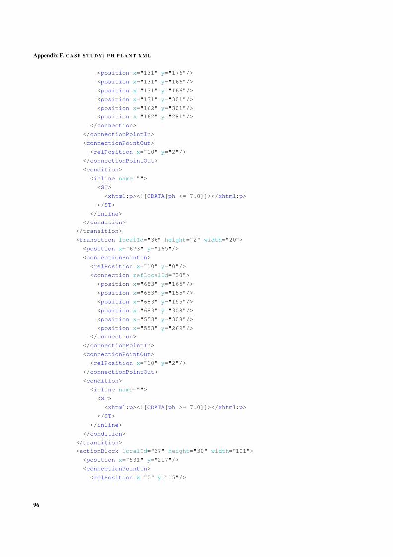
Appendix F. C A S E S T U DY: P H P L A N T X M L
<position x="131" y="176"/>
<position x="131" y="166"/>
<position x="131" y="166"/>
<position x="131" y="301"/>
<position x="162" y="301"/>
<position x="162" y="281"/>
</connection>
</connectionPointIn>
<connectionPointOut>
<relPosition x="10" y="2"/>
</connectionPointOut>
<condition>
<inline name="">
<ST>
<xhtml:p><![CDATA[ph <= 7.0]]></xhtml:p>
</ST>
</inline>
</condition>
</transition>
<transition localId="36" height="2" width="20">
<position x="673" y="165"/>
<connectionPointIn>
<relPosition x="10" y="0"/>
<connection refLocalId="30">
<position x="683" y="165"/>
<position x="683" y="155"/>
<position x="683" y="155"/>
<position x="683" y="308"/>
<position x="553" y="308"/>
<position x="553" y="269"/>
</connection>
</connectionPointIn>
<connectionPointOut>
<relPosition x="10" y="2"/>
</connectionPointOut>
<condition>
<inline name="">
<ST>
<xhtml:p><![CDATA[ph >= 7.0]]></xhtml:p>
</ST>
</inline>
</condition>
</transition>
<actionBlock localId="37" height="30" width="101">
<position x="531" y="217"/>
<connectionPointIn>
<relPosition x="0" y="15"/>
96

<connection refLocalId="25">
<position x="531" y="232"/>
<position x="521" y="232"/>
<position x="521" y="232"/>
<position x="519" y="232"/>
</connection>
</connectionPointIn>
<action localId="0" qualifier="P1">
<relPosition x="0" y="0"/>
<inline>
<ST>
<xhtml:p><![CDATA[vphp :=TRUE;]]></xhtml:p>
</ST>
</inline>
</action>
</actionBlock>
<actionBlock localId="38" height="30" width="106">
<position x="248" y="218"/>
<connectionPointIn>
<relPosition x="0" y="15"/>
<connection refLocalId="23">
<position x="248" y="233"/>
<position x="232" y="233"/>
<position x="232" y="233"/>
<position x="237" y="233"/>
</connection>
</connectionPointIn>
<action localId="0" qualifier="P1">
<relPosition x="0" y="0"/>
<inline>
<ST>
<xhtml:p><![CDATA[vphm := TRUE;]]></xhtml:p>
</ST>
</inline>
</action>
</actionBlock>
</SFC>
</body>
</pou>
97


This work is financed by the ERDF - European Regional Development Fund through the COMPETE Pro-gramme (operational programme for competitiveness) and by National Funds through the FCT - Fundação paraa Ciência e a Tecnologia (Portuguese Foundation for Science and Technology) within project FCOMP-01-0124-FEDER-028923