VII Simpósio Brasileiro de Arquitetura de Computadores -Processamento de Alto Desempenho 581

A Tool for Modeling and Simulation of Computer Architectures Using1

Petri Nets

Marcelo H. Cintra1

Wilson V. Ruggiero11

'Laboratório de Sistemas Integráveis e-mail: mcintra@lsi.usp.br

11Laboratório de Arquiteturas e Redes de Computador e-mail: wilson@larc.usp.br

Universidade de São Paulo

Abstract

The developments in the field of computer architecture, especially parallel systems, lead to the design of even more complex architectures, making it difficult to take decisions that would increase the performance of the system. In order to analyze objectively the advantages of ditferent architectural choices, it is important to have modeling and analysis techniques and tools that can efficiently acquire data about the system's performance.

Petri nets have been used successfully as a modeling tool for computer architectures. However, the analysis of the complex nets needed to model real systerns has become a lirniting factor for using Petri nets. To efficiently use Petri nets for modeling these complex systems, one needs powerful computer simulation tools.

In this pape r we present the program RP _SIM, an object oriented tool for the simulation ofPetri nets. We use this simulator to analyze a simple computer architecture model, showing the viability o f the use o f Petri nets, together with the tool presented, to model general computer architectures.

1 Introduction

In the pursuit of more powerful computers, many ditferent architectures have been proposed. Those computers have great ditferences with respect to the number and type of processors, memory configuration and hierarchy, interconnection network, synchronization support, and many other factors that atfect the overall performance of the computer system.

To make an objective analysis of the advantages of a given architecture over other proposals, both to help in the design and to compare existing machines, it is convenient to use models and simulations. With this approach one can accelerate the design of new machines and reduce the need for experiments with real systems, which are usually expensive and time-consurning.

1 This research was supported in part by Conselho Nacional de Desenvolvimento Cientifico e Tecnológico (CNPq - Brazil)

582 XV Congr~ da s-ade "'"'""do Computação

Petri nets have been used successfully to ode! computer arehitectures. This technique has proven itself adequate to model th parallelism and conflict[ll, two important eharaeteristies present in modem compu r systems. Besides the capacity of the original net to model the flow of control and ata, extensions sueh as timed and stoehastie Petri nets are also powerful techniqu for analyzing the performance of systems. Zuberek[l6) used timed Petri nets to get pe ormance indices of some computer arehitectures. Shaefer{l4] used basie Petri nets to m el the control of massively parallel computers. Petri nets can also be used to modela eroprocessor's internai operation, as was done by Razouk[ll).

The complexity o f the analysis o f the Petri ets ereated to model real computer systems requires the use of computer simulation too s. Many tools for that purpose have been proposed in the literature, as in [2] [3] [6] [9].-lfhese tools were developed to run in different platforms and have distinct features and f"sphical user interfaces. We believe that an important feature that will prove to be ext~ely useful is the possibility of step­by-s~ep simulation, as is done in [6). By doing ste -by-step simulation, one can analyze very complex Petri nets without the need to u traditional analytical methods that involve the computation of the net's reaehability se~t, whose complexity tends to grow exponentially with the problem size.

In this paper we present the simulator RP _ S as an object oriented tool that can solve complex Petri nets, step-by-step, in non- xpensive personal computers. The organization of this paper is as follows: in section we present a short introduction to Petri nets, in section 3 we present an overview o f the simulator and its features, and in seetion 4 we use the simulator to analyze a queuing system MIM/2/B. In section 5 we use the simulator in a simple model of a compute arehitecture, mostly to demonstrate the potential of the use of Petri net modeling an the tool presented. In section 6 we present some conclusions and final remarks and w discuss some desired improvements in the program, which shall be implemented in the ture.

2 Petri Nets

A basic Petri net may be defined as a gr ph created with three sets: a set of places P, a set of transitions T and a set of dir~ted ares A Ares rnay link places to transitions o r transitions to places. A formal defini on o f a basic Petri net would be:

PN = {P, T, A} P = {Pl. P2. P3 •... , Pn} T = {ti, t2, t3, ... , tm} A c {TxP} u {PxT} A place Pi is said to be an input place o a given transition tj if there is an are

directed from Pi to tj. Sirnilarly a place Pi is said o be an output place of tj if there is a directed are from tj to Pi·

l(t) = {p I (p, t) e A} O(t) = {p I (t, p) e A} Besides the sets defined above, a marked etri net is also identified by a marking

M. Tokens are assigned to places and the markin , in a given state o f the net is defined by the set o f ali tokens currently assigned to each pia in the net:

Ms = {msl, ms2, msJ, ... , msn}

VII Simpósio Brasileiro de Arquitetura de Computadores· Processamento de Alto Desempenho 583

where msi represents the number of tokens in place i in the marking M5. Mo represents the initial state o f the net. o

The execution o f a Petri net is done by the firing o f transitions. A transition may fire if it is enabled, a situation that happens when ali its input places have at least one token. The firing of a transition involves removing a token from ali the input places and putting a token in each output place, thus generating a new marking M. Based on this definition, one can see that the number of tokens in the net changes when I l(tj) I ~I O(tj) I.

With respect to these basic transitions, the firing is immediate and in the case that two transitions be in conflict, i.e., both are enabled in a given marking M5 and the firing of one transition disables the other, the choice ofwhich one to fire is non deterrninistic.

Many extensions have been proposed to increase the modeling power o f the basic Petri nets. Some extensions are: • Ares with multiplicity k: in this case a transition is enabled only ifthe number oftokens in each ofits input places is greater than or equal to the multiplicity ofthe are linking the place to the transition. The firing of a transition, then, involves removing from the input places as many tokens as the multiplicity o f the incoming are, and assigning to the output places as many tokens as the multiplicity o f the outgoing are. •lnhibitor ares: inhibitor ares indicate that the absence oftokens in an input place enables the transition and the presence of a token disables the transition. The firing of the transition follows the same rules ofthe basic net except that the input place connected to the inhibitor are remains untouched. • Colored nets: in this special net, the tokens may be assigned an identification (color) and the enabling of a transition may depend on the colors of the tokens in the input places. The firing of a transition may remove tokens of a given color from the input places and put tokens of a different color in the output places, thus changing the colors ofthe tokens as they move through the net. • Timed nets: the time factor may be introduced in the places so that a new token is only available to a transition after some time delay. More commonly, one associates time to transitions in which case there are two possibilities: a transition may require a given enabling time, after which the firing is immediate; or the transition may tire as soon as it is enabled but the firing may take some time. • Stochastic nets: in this case one associates a random time to the firing or enabling tir1e o f transitions. In the GSPN model, transitions can also be defined as immediate, and they have priority of firing over transitions with non zero time. There is also the DSPN net that is a GSPN net that can handle both random and deterrninistic firing times.

For more details about Petri nets the reader is referred to Peterson's book[IOJ.

3 The Simulator RP _SIM

The simulator RP _SIM is a tool for simulation o f Petri nets that is capable o f dealing with deterrninistic and stochastic Petri nets (DSPN) and which also supports colored tokens and ares with multiplicity. This program was initially developed by Sangiorgio!I2J and is currently being improved and extended. Different from the majority of the existing tools, this simulator presents an open architecture, allowing the user to extend the tool by adding its own code, written in a language developed with some features offered by the object oriented prograrnming language C++[ISJ. This particular

584 da Sociedade Brasileira de Computação

feature of the sirnulator makes it highly tlexible, in easing, however, the complexity of its use.

Due to its open architecture, the sirnulator is not an executable program, but consists of codes written in C++ - RP SIM.CP and SIM OBS.H - that must be compiled along with the user' s code, ~ed SIM.H. The executable program generated may be run in PC-type computers, 'thout demanding requirements of hardware and software.

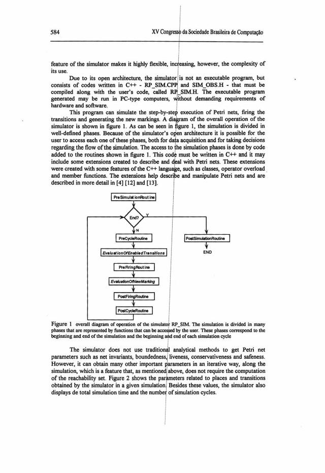
This program can sirnulate the step-by-ste execution of Petri nets, firing the transitions and generating the new markings. A di of the overall operation of the sirnulator is shown in figure 1. As can be seen in gure I, the sirnulation is divided in well-defined phases. Because of the sirnulator's o n architecture it is possible for the user to access each one ofthese phases, both for d acquisition and for taking decisions regarding the flow ofthe simulation. The access to he simulation phases is done by code added to the routines shown in figure I. This codp must be written in C++ and it may include some extensions created to describe and ~ with Petri nets. These extensions were created with some features of the C++ language, such as classes, operator overload . and member functions. The extensions help d · and manipulate Petri nets and are described in more detail in [4] [12] and [13].

END

Figure 1 overall diagram of opcration of the simulator RP SIM. The simulation is divided in many I -

phases that are rcpresentcd by functions that can be ~ by lhe user. These phases correspond to the beginning and end of the simulation and the beginning aiKI end of each simulation cycle

The simulator does not use traditio analytical methods to get Petri net parameters such as net invariants, boundedness liveness, conservativeness and safeness. However, it can obtain many other important arameters in an iterative way, along the simulation, which is a feature that, as mentioned above, does not require the computation of the reachability set. Figure 2 shows the par eters related to places and transitions obtained by the sirnulator in a given simulation Besides these values, the sirnulator also disptays de total simulation time and the numbe o f simulation cycles.

VII Simpósio Brasileiro de Arquitetura de Computadores -Processamento de Alto Desempenho 585

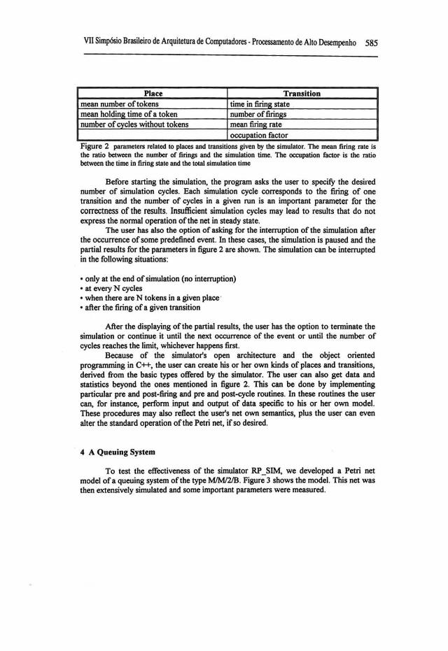
Place Transition mean number oftokens time in firing state mean holding time o f a token number offirings number o f cycles without tokens mean firing rate

occupation factor .. Ftgure 2 parameters related to places and transitJons giVen by the s•mulator. The mean firing rate is

the ratio between the number of firings and the simulation time. The occupation facto!' is lhe ratio between lhe time in firing state and the total simulation time

Before starting the simulation, the program asks the user to specifY the desired number of simulation cycles. Each simulation cycle corresponds to the firing of one transition and the number of cycles in a given run is an important parameter for the correctness o f the results. Insufficient simulation cycles may lead to results that do not express the normal operation ofthe net in steady state.

The user has also the option of asking for the interruption of the simulation after the occurrence o f some predefined event. In these cases, the simulation is paused and the partia! results for the parameters in figure 2 are shown. The simulation can be interrupted in the following situations:

• only at the end of simulation (no interruption) • at every N cycles • when there are N tokens in a given place · • after the firing o f a given transition

After the displaying o f the partia! results, the user has the option to termina te the simulation or continue it until the next occurrence of the event or until the number of cycles reaches the limit, whichever happens first .

Because of the simulator's open architecture and the object oriented prograrnming in C++, the user can create his or her own kinds of places and transitions, derived from the basic types offered by the simulator. The user can also get data and statistics beyond the ones mentioned in figure 2. This can be done by implementing particular pre and post-firing and pre and post-cycle routines. In these routines the user can, for instance, perforrn input and output of data specific to his or her own model. These procedures may also reflect the user's net own semantics, plus the user can even alter the standard operation o f the Petri net, i f so desired.

4 A Queuing System

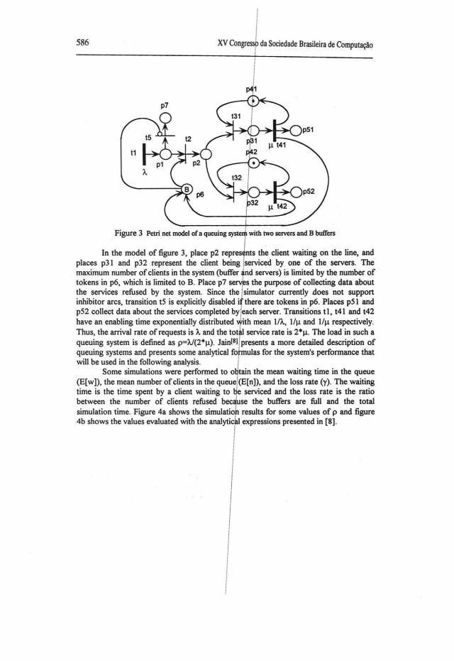
To test the effectiveness of the simulator RP _SIM, we developed a Petri net model ofa queuing system ofthe type M/M/2/B. Figure 3 shows the model. This net was then extensively simulated and some important parameters were measured.

586 da Sociedade Brasileira de Computação

In the model of figure 3, place p2 repr nts the client waiting on the Jine, and places p31 and p32 represent the client being serviced by one of the servers. The maxirnum number of clients in the system (butfer d servers) is lirnited by the number of tokens in p6, which is limited to B. Place p7 se 1 the purpose of collecting data about the services refused by the system. Since the sirnulator currently .does not support inhibitor ares, transition tS is explicitly disabled · there are tokens in p6. Places pS 1 and p52 collect data about the services completed by each server. Transitions t1, t41 and t42 have an enabling time exponentially distributed "th mean 1/Ã., 111-1 and 1/1-1 respectively. Thus, the arrival rate ofrequests is À. and the tot service rate is 2*1-1· The load in such a queuing system is defined as p=Ã./(2*!-1). Jain[BJ presents a more detailed description of queuing systems and presents some analytical fo ulas for the system's performance that will be used in the following analysis.

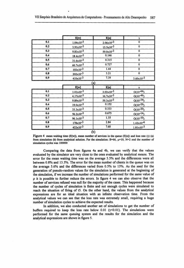
Some simulations were performed to o tain the mean waiting time in the queue (E[w]), the mean number ofclients in the queue (E[n)), and the loss rate (y). The waiting time is the time spent by a client waiting to serviced and the loss rate is the ratio between the number of clients refused se the butfers are full and the total simulation time. Figure 4a shows the simulatio results for some values of p and figure 4b shows the values evaluated with the analytic expresslons presented in [8].

VII Simpósio Brasileiro de Arquitetura de Computadores • Processamento de Alto Desempenho 587

E[w) Efn) y

0.1 1.04xl0·3 2.06xl0·3 o

0.1 3.91xto·3 1S.Sx1o·3 o

0.3 9.81xto·3 S9.0xlo·3 o

0.4 18.4x1o·3 0. 146 o

o.s 31.6xl0"3 0.31S o

0.6 60.7x1o·3 0.727 o

0.7 102x1o·3 1.44 o

0.8 202x1o·3 3.21 o

0.9 410x1o·3 7.39 3.6oxio·3

(a)

Elwl Elnl y

0.1 1.01x1o·3 2.02x1o·3 0(10-66) O.l 4.17x1o·3 16.7x1o·3 ooo-46> 0.3 9.89x1o·3 S9.3x1o·3 ooo·34>

0.4 19.0xl0"3 O.IS2 ooo·26> o.s 33.3x1o·3 0.333 ooo·20> 0.6 S6.2xl0"3 0.67S 0<1o·14> 0.7 96.1x1o·3 1.3S 0<1o·10)

0.8 178xl0"3 2.84 1.42xlo-6 0.9 422x1o·3 7.60 1.81x10"3

(b) Figure 4 mean waiting time (E[w)), mean numbcr of services in lhe queue (E[n]) and loss rate (y) (a) from simulation (b) from analytical solution. For lhe simulation: 8=66, 14=10, N"'l and lhe numbcr of simulation cycles was 100000

Comparing the data from figures 4a and 4b, we can verify that the values evaluated by the simulator are very close to the ones evaluated by analytical means. The error for the mean waiting time was on the average 5.5% and the differences were ali between 0.8% and 13.5%. The error for the mean number of clients in the queue was on the average 5.6% and the differences varied from 0.5% to 13%. As the seed for the generation of pseudo-random values for the simulation is generated at the beginning of the simulation, ifwe increase the number of simulations performed for the same value of p it is possible to further reduce the errors. In figure 4 we can also observe that the number o f services refused was null for the majority o f the cases. This happened because the number of cycles of simulation is finite and not enough cycles were simulated to reach the situation of firing of tS. On the other hand, the values from the analytical expressions are for an ideal situation with an infinite observation time. From the analytical values we can see that the loss rate was extremely small, requiring a huge number o f simulation cycles to achieve the expected results.

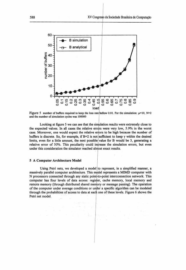
In addition, we also conducted another set of simulations to get the number of buffers required to keep the loss rate below 0.01 (y<O.Ol). The simulations were performed for the same queuing system and the results for the simulation and the analytical expressions are shown in figure S.

588 XV Congr da Sociedade Brasileira de Computação

60

-e- B simulation 50 B analytical -e-

~40 ~ J:l

Õ30 .... ~ § 20 c:

10

o I'- LOCO LO Ol .,.... . """ . co c)

c) o . o c) o

Figure 5 number of buffers required to keep lhe loss rale bellow 0.0 I. For lhe simulation: j!• IO, N=2 and lhe number of simulation cycles was 100000

Looking at figure 5 we can see that the si lation results were extremely close to the expected values. In ali cases the relative err rs were very low, 5.90/o in the worst case. Moreover, one would expect the relative e ors to be high because the number of buffers is discrete. So, for exarnple, if B=2 is not sufficient to keep y within the desired limits, even for a little arnount, the next possible value for B would be 3, generating a relative error of 50%. This peculiarity could in rease the simulation errors, but even under this consideration the simulator reached ai ost exact results.

!5 A Computer Arcbitecture Model

Using Petri nets, we developed a model to represent, in a simplified manner, a massively parallel computer architecture. This m · del represents a MIMD computer with N processors connected through any static poi~to-point interconnection network. This computer has four leveis of data access: regis er, cache memory, local memory and remote memory (through distributed shared me ory or message passing). The operation of the computer under average conditions or un er a specific algorithm can be modeled through the probabilities o f access to data at eac one o f these leveis. Figure 6 shows the Petri net model.

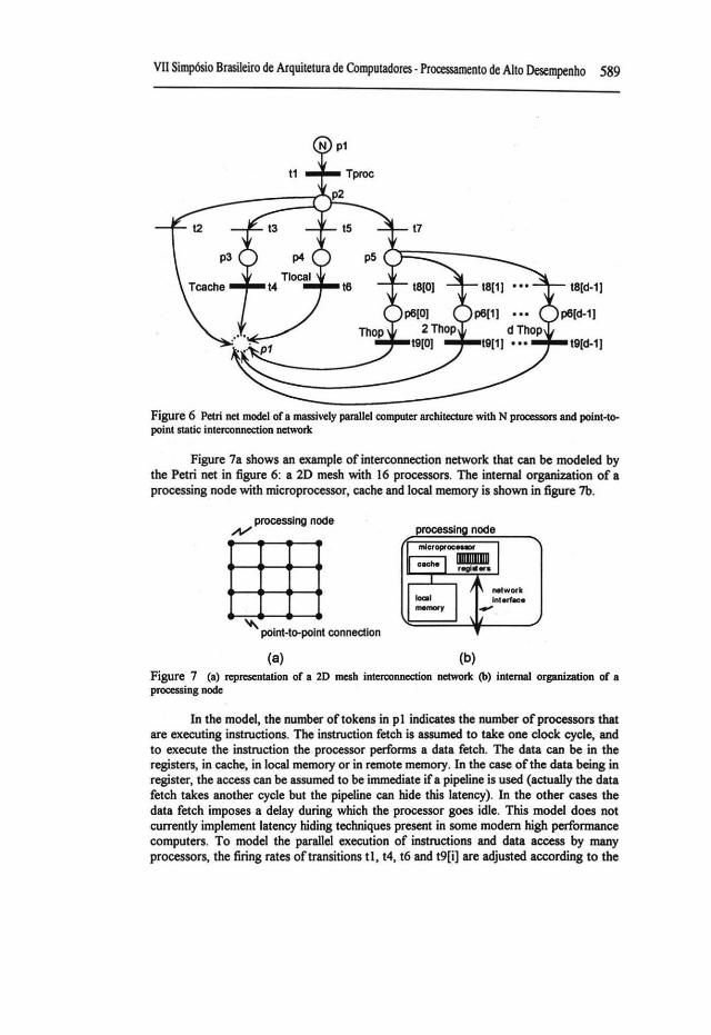
VII Simpósio Brasileiro de Arquitetura de Computadores -Processamento de Alto Desempenho 589

Figure 6 Petri net model of a massively parallel computer architecture with N processors and point-to­point static interconnection networlc

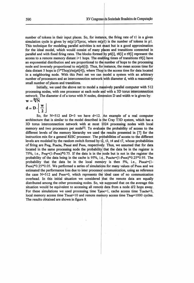
Figure 7a shows an example of interconnection network that can be modeled by the Petri net in figure 6: a 20 mesh with 16 processors. The internai organization of a processing node with microprocessor, cache and local memory is shown in figure 7b.

processing node A/

Em point-to-polnt connectlon

(a) (b) Figure 7 (a) represcntation of a 20 mcsh interconncction networlc (b) internai organization of a processing node

In the model, the number of tokens in p 1 indicates the number of processors that are executing instructions. The instruction fetch is assumed to take one clock cycle, and to execute the instruction the processor performs a data fetch. The data can be in the registers, in cache, in local memory or in remote memory. In the case ofthe data being in register, the access can be assumed to be immediate if a pipeline is used (actually the data fetch takes another cycle but the pipeline can hide this Jatency). In the other cases the data fetch imposes a delay during which the processor goes idle. This model does not currently implement latency hiding techniques present in some modem high performance computers. To model the parallel execution of instructions and data access by many processors, the firing rates oftransitions tl, t4, t6 and t9[i] are adjusted according to the

590 XV Congresso da Sociedade Brasileira de Computação

number of tokens in their input places. So, for instan~, the firing rate of tl in a given simulation cycle is given by m(pl)ffproc, where m(pf ) is the number of tokens in pl. This technique for modeling parallel activities is not but is a good approximation for the ideal model, which would consist of many p ces and transitions connected in parallel and with fixed firing rates. The blocks formed y p6[i], t8[i] e t9[i] represent the access to a remo te memory distant i+ I hops. The e ling times o f transitions t9[i] have an exponential distribution and are proportional to th number o f hops to the processing node and inversely proportional to m(p6[i]). Thus, for instance, the mean access time for data distant 5 hops is (5•Thop)/m(p6[4]), where ThoA is the access time for data located in a neighboring node. With this Petri net we can lnodel a system with an arbitrary number ofprocessors and an interconnection netwoí'th diameter d, with a reasonably small number o f places and transitions.

lnitially, we used the above net to modela ively parallel computer with 512 processing nodes, with one processor at each node d with a 3D torus intercoMection network. The diameter d o f a torus with N nodes, dim nsion D and width w is given by:

w = J>JN

d=n·l~J So, for N=Sl2 and D=3 we have d=l2. ~ example of a real computer

architecture that is similar to the model described is f!l: Cray T3D system, which has a 3D torus interconnection network with at most ~024 processing nodes with local memory and two processors per nodeiSJ. To evalua e the probability of access to the different leveis of the memory hierarchy we used e results presented in [7] for the instruction mix for a general RISC processor. The pr babilities of acce~s to the different leveis are modeled by the random switch formed by ·, t3, t4 and t7, whose probabilities of firing are Preg, Pcache, Plocal and Prem, respective y. Thus, we assumed that for data located in the same processing node the probability that the data be in the register is 75%, i.e., Preg=(l-Prem)•0.7S. Ifthe datais in the ode but is not in the register the probability of the data being in the cache is 95%, i. ., Pcache=(l-Prem)•0.25•0.95. The probability that the data be in the local mem ry is then 5%, i.e., Plocal={l ­Prem)•0.2S•0.05. We performed a series ofsimulati ns for many values ofPrem and we estimated the performance loss due to inter processo communication, using as reference the case N=512 and Prem=O, which represents th ·ideal case of no communication overhead. In this initial situation we considered hat the remote data are equally distributed among the other processing nodes. So, supposed that on the average this situation would be equivalent to accessing ali remot data from a node d/2 hops away. For these simulations we used processing time Tpioc=( cache access time Tcache=3, local memory access time nocai=lO and remote merbory access time Thop=IOOO cycles. The results obtained are shown in figure 8.

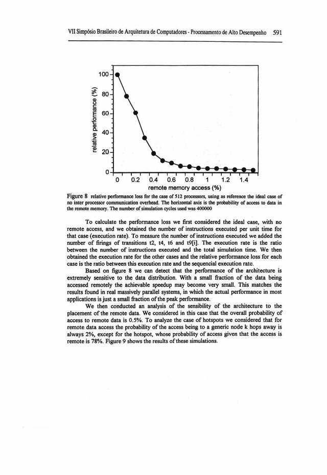
VII Simpósio Brasileiro de Arquitetura de Computadores- Processamento de Alto Desempenho 591

100

~ 80 ~ c (1J

E 60 .g ~ 40 Q) > i e 20

o 0.2 0.4 0.6 0.8 1 1.2 1.4 remota memory access (%)

Figure 8 relative perfonnance Joss for lhe case of S 12 processors, using as reference lhe ideal case of no inter processor c:ommunlc:ation overhead. Tbe horizontal axis is lhe probability of access to data in lhe remotc memory. Tbe nwnber of simulation cycles used was 400000

To calculate the perfonnance loss we first considered the ideal case, with no remote access, and we obtained the number of instructions executed per unit time for that case (execution rate). To measure the number ofinstructions executed we added the number of firings of transitions t2, t4, t6 and t9(i]. The execution rate is the ratio between the number of instructions executed and the total simulation time. We then obtained the execution rate for the other cases and the relative perfonnance loss for each case is the ratio between this execution rate and the sequencial execution ratc.

Based on figure 8 we can detect that the perfonnance of the architecture is extremely sensitive to the data distribution. With a small fraction of the data being accessed remotely the achievable speedup may become very small. This matches the results found in real massively parallel systems, in which the actual perfonnance in most applications is just a small fraction o f the peak perfonnance.

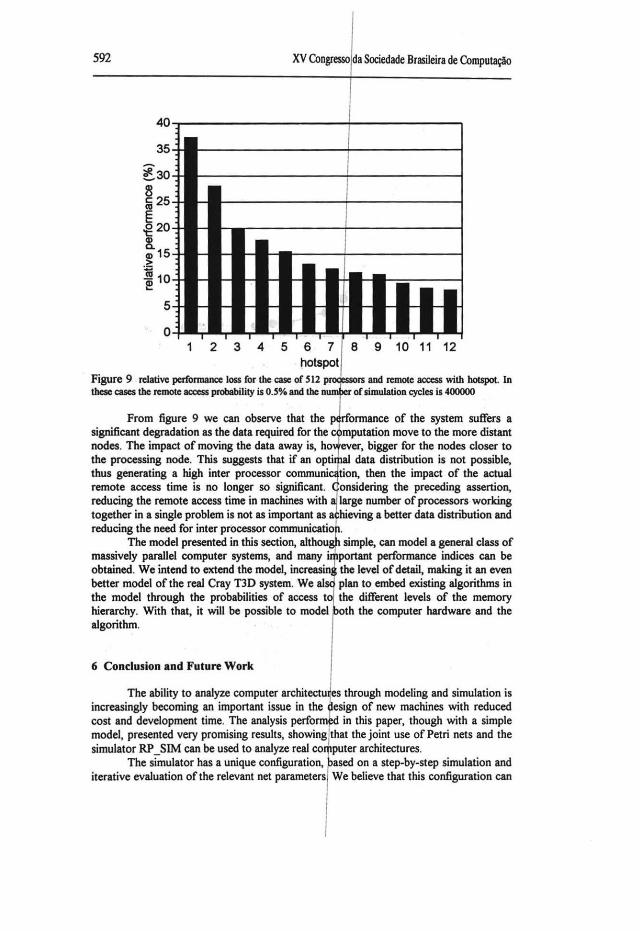
We then conducted an analysis of the sensibility of the architecture to the placement ofthe remote data. We considered in this case that the overall probability of access to remote data is 0.5%. To analyze the case of hotspots we considered that for remote data access the probability o f the access being to a generic node k hops away is always 2%, except for the hotspot, whose probability of access given that the access is remote is 78%. Figure 9 shows the results ofthese simulations.

592 X.V Congresso da Sociedade Brasileira de Computação

40,-------------------+-----------~

35

~30 -g25 111

E .g 20

~15 -~ ~ 10 e

5

o

r-

-

-

-

-

1

1-

r- - ~

r- -;- r-

r- - r-

2 3 4 5

r- - r-

r- - r- - r- ~

"" 6 7 8 9 10 11 12 tlotspot

Figure 9 rdative performance Ioss for lhe case of 512 proc essors and rcmote acx:ess with hotspot. In these cases lhe remote acx:ess probability is O.S% and lhe num ler of simulation cycles is 400000

From figure 9 we can observe that the p rformance of the system suffers a significant degradation as the data required for the o mputation move to the more distant nodes. The impact of moving the data away is, hov ever, bigger for the nodes closer to the prooessing node. This suggests that if an opti fuu data distribution is not possible, hus generating a high inter processor communiel tion, then the impact of the actual

remote aocess time is no longer so significant. ( onsidering the preoeding assertion, reducing the remote access time in machines with a large number o f prooessors working together in a single problem is not as important as a hieving a better data distribution and reducing the need for inter processor oommunicatioll.

The model presented in this section, althou~ 11 simple, can model a general class of massively parallel oomputer systems, and many ir portant performance indioes can be obtained. We intend to extend the model, increasin the levei of detail, making it an even better model of the real Cray TIO system. We aiS< plan to embed existing algorithms in the model through the probabilities of acoess to the different leveis of the memory hierarchy. With that, it will be possible to model both the oomputer hardware and the algorithm.

6 Condusion and Future Work

The ability to analyze oomputer architectu~s through modehng and s1mulauon 1s increasingly beoorning an important issue in the esign of new machines with reduoed oost and development time. The analysis perform in this paper, though with a simple model, presented very prornising results, showing that the joint use o f Petri nets and the simulator RP _SIM can be used to analyze real oo pu ter architectures.

The simulator has a unique configuration, ased on a step-by-step simulation and iterative evaluation ofthe relevant net parameters We believe that this oonfiguration can

VII Simpósio Brasileiro de Arquitetura de Computadores • Processamento de Alto Desempenho 593

solve nets with a higher degree of complexity than current Petri net tools can. Despite this unique configuration, the correctness of the simulator was verified through the analysis o f a queuing system, whose analytical solution is known.

Though the simulator proved to be a powerful tool, its user interface still needs some refinements, specially the addition of a graphical user interface. The fact that the simulator uses an unusual method for solving the Petri net, does not discard the possibility of inclusion, in future versions, of traditional methods based on the reachability set. These additions would greatly improve the simulator's power and ease of use.

With the current features and future improvements we hope to offer a powerful tool both for teaching purposes and for helping in the development of new complex computer architectures.

References

[1] Agerwala, T., "Putting Petri Nets to Work", Computer, December 1979, pp. 85-94

[2] Atamna, Y., "RPTS: A Tool for Stochastic Timed Petri Nets", Proceedings ofthe 5th Intemational Workshop on Petri Nets and Performance Models, 1993

[3) Ceska, M. and Skacel, M., "Petri Net Tool PESIM: the tool for Petri net drawing, simulation and analysis", Proceedings of the 5th Intemational Workshop on Petri Nets and Performance Models, 1993

[4) Cintra, M. H., Manual do Usuário do Programa RP_SIM- Simulador de Redes de Petri Interpretadas, Technical Report, Universidade de São Paulo, 1994

[5] Cray, Cray T3D System Architecture Overview Manual, Cray Research, 1993

[6] Gellot, F., Carre-Menetrier, V., Lecolier, G. V., "PETRILAM: A Tool for Petri Nets Analysis and Simulation", Proceedings ofthe 5th lntemational Workshop on Petri Nets and Performance Models, 1993

[7] HeMessy, J. and Patterson, D., Computer Architecture a Quantitative Approach, Morgan Kaufinann, 1990

[8) Jain, R., The Arl oj Computer Systems Performance Analysis: Techniques for Experimental Design, Measurement, Simulation, and Modeling, John Wiley & Sons, 1992

[9] Lindemann, C., "DSPNexpress: A Software Package for the Efficient Solution of Deterrninistic and Stochastic Petri Nets", Proceedings ofthe 5th lntemational Workshop on Petri Nets and Performance Models, 1993

[10] Peterson, J. L., Petri Net Theoryand the Mode/ingojSystems, Prentice-Hall, 1981