Universidade ederalF de Santa Catarina Biblioteca ... · for the Embedded Parallel Operating System...

Universidade Federal de Santa CatarinaBiblioteca Universitária

Davi Resner

Performance Evaluation of the Trustful Space-Time Protocol

Florianópolis

2018

Davi Resner


Dissertatação submetida ao Programade Pós-Graduação em Ciência da Com-putação da Universidade Federal deSanta Catarina para a obtenção doGrau de Mestre em Ciência da Com-putação.Orientador: Prof. Dr. Antônio Au-gusto Fröhlich

Florianópolis

2018

Ficha de identificação da obra elaborada pelo autor, através do Programa de Geração Automática da Biblioteca Universitária da UFSC.

Resner, Davi Performance Evaluation of the Trustful SpaceTime Protocol / Davi Resner ; orientador, AntônioAugusto Fröhlich, 2018. 190 p.

Dissertação (mestrado) - Universidade Federal deSanta Catarina, Centro Tecnológico, Programa de PósGraduação em Ciência da Computação, Florianópolis,2018.

Inclui referências.

1. Ciência da Computação. 2. Protocolos deComunicação. 3. Internet das Coisas. 4. Design crosslayer. 5. Avaliação de desempenho. I. Fröhlich,Antônio Augusto. II. Universidade Federal de SantaCatarina. Programa de Pós-Graduação em Ciência daComputação. III. Título.

Davi Resner


Esta dissertação foi julgada adequada para obtenção do título de mestre e aprovada em sua forma final pelo Programa de Pós-Graduação em Ciência da Computação.

Florianópolis, 02 de março de 2018.

__________________________Prof. José Luís Almada Güntzel, Dr.

Coordenador do Programa

Banca Examinadora:

_________________________Prof. Antônio Augusto Fröhlich, Dr.

Universidade Federal de Santa CatarinaOrientador

_________________________Prof. Wolfgang Schröder-Preikschat, Dr.

Friedrich-Alexander-Universität

_________________________Prof. Antonio Alfredo Ferreira Loureiro, Dr.

Universidade Federal de Minas Gerais

_________________________Prof. Gustavo Medeiros de Araujo, Dr.Universidade Federal de Santa Catarina

_________________________Prof. Paulo José de Freitas Filho, Dr.

Universidade Federal de Santa Catarina

À Julia.

Abstract

Wireless Sensor Networks (WSN) have been implemented in manydi�erent forms over the years. Buildings, homes, farms, rivers, theweather, assembly lines, and many more physical environments, can allbe monitored and sometimes controlled by a wireless network of cheapcomputing devices equipped with di�erent sensors and actuators. Asthese networks get connected to the Internet of Things (IoT), it is evermore important that they operate trustfully, with carefully-designedand -implemented domain-oriented operating systems and network pro-tocols.The Trustful Space-Time Protocol (TSTP) is a cross-layer WSN pro-tocol designed to deliver authenticated, encrypted, timed, and geo-referenced messages containing data compliant with the InternationalSystem of Units (SI) in a resource-e�cient way. By integrating shareddata from multiple networking services into a single communicationinfrastructure, TSTP is able to eliminate replication of informationacross services, achieving small overhead in terms of control messages.However, the complexity of TSTP's features, its broad range - fromapplication to Medium Access Control, - and its experimental naturebring diverse requirements beyond those usually considered in mostsoftware designs.In this dissertation, the protocol design of TSTP is presented in de-tail, with a description of the message formats and algorithms used formedium access control, geographic routing, spatial localization, timesynchronization, and security. Then, an implementation is developedfor the Embedded Parallel Operating System (EPOS) and the EPOS-Mote III WSN platform. To avoid a monolithic implementation ofthe cross-layer approach, a component-based design is used, explor-ing template metaprogramming techniques to adapt and combine basicbuilding blocks. An event-driven architecture that makes use of zero-copy bu�ers and metadata is used to handle crosscutting concerns. Thedesign and implementation are assessed with experiments on the EPOS-Mote III platform, with a port for the OMNeT++ simulator, and withan analytic model of network behavior. With the experiments and datacollected from various evaluation tools, parameters of the protocol areadjusted and optimized, improving TSTP and taking it one step closerto its goal of being a complete, e�cient solution for IoT-ready WSNs.

Keywords: Cross-layer design; Performance evaluation; Communi-

cation protocols; Internet of Things; Wireless Sensor Networks

Resumo

Redes de Sensores Sem Fios (RSSF) têm sido implementadas de muitasformas diferentes ao longo dos últimos anos. Prédios, casas, fazendas,rios, o clima, chãos de fábrica, e muitos outros tipos de ambiente, podemtodos ser monitorados e controlados por uma rede sem �os compostade dispositivos computacionais baratos equipados com diferentes sen-sores e atuadores. Com estas redes conectando-se à Internet das Coisas(IoT, do inglês Internet of Things), torna-se cada vez mais importanteque as mesmas operem de maneira con�ável, com sistemas operacio-nais e protocolos de comunicação orientados ao domínio de aplicação ecuidadosamente implementados.O Trustful Space-Time Protocol (TSTP) é um protocolo cross-layerpara RSSF projetado para enriquecer dados com semântica de unida-des do Sistema Internacional (SI), autenticação, criptogra�a, tempora-lidade e georeferenciamento de forma e�ciente. Através da integraçãode dados compartilhados por múltiplos serviços de rede em uma únicainfraestrutura de comunicação, TSTP é capaz de eliminar a replica-ção de informação entre serviços, atingindo um sobrecusto modesto emtermos de mensagens de controle. Porém, a complexidade das funciona-lidades do TSTP, seu amplo escopo - da aplicação ao controle de acessoao meio, - e sua natureza experimental trazem requerimentos diversos,além daqueles normalmente considerados na maioria dos projetos desoftware.Nesta dissertação, o projeto de protocolo do TSTP é exposto em deta-lhes, com uma descrição dos formatos de mensagem e algoritmos usadospara controle de acesso ao meio, roteamento geográ�co, localização es-pacial, sincronização temporal e segurança. Então, uma implementaçãodesenvolvida para o Embedded Parallel Operating System (EPOS) e aplataforma de RSSF EPOSMote III é apresentada. Para evitar uma im-plementação monolítica da abordagem cross-layer, um projeto baseadoem componentes é utilizado, explorando técnicas de metaprogramaçãocom templates para adaptar e combinar blocos básicos. Uma arquite-tura orientada a eventos que gerencia bu�ers enriquecidos com meta-dados sem gerar cópias de memória é aplicada para tratar de requisitostransversais. O projeto e a implementação do protocolo são avaliadoscom experimentos na plataforma EPOSMote III, com um porte para osimulador OMNeT++ e com um modelo analítico de comportamentoda rede. Com base nos experimentos e dados coletados por meio de

várias ferramentas de avaliação, parâmetros do protocolo são ajustadose otimizados, melhorando o TSTP e trazendo-o um passo mais pertode seu objetivo de prover uma solução completa e e�ciente para RSSFintegradas à IoT.

Palavras-chave: Design cross-layer; Avaliação de desempenho; Pro-tocolos de comunicação; Internet das Coisas; Redes de Sensores SemFios

Resumo Expandido

IntroduçãoRedes de Sensores Sem Fios (RSSF) têm sido implementadas de muitasformas diferentes ao longo dos últimos anos. Prédios, casas, fazendas,rios, o clima, chãos de fábrica, e muitos outros tipos de ambiente, podemtodos ser monitorados e controlados por uma rede sem �os compostade dispositivos computacionais baratos equipados com diferentes sen-sores e atuadores. Com estas redes conectando-se à Internet das Coisas(IoT, do inglês Internet of Things), torna-se cada vez mais importanteque as mesmas operem de maneira con�ável, com sistemas operacionaise protocolos de comunicação orientados ao domínio e cuidadosamenteimplementados. Este trabalho avalia e melhora o Trustful Space-TimeProtocol (TSTP) (RESNER; FRÖHLICH, 2015a; RESNER; ARAUJO; FRÖH-LICH, 2017), trazendo-o um passo mais perto de seu objetivo de proveruma solução completa e e�ciente para RSSF integradas à IoT.A IoT destaca desa�os que estiveram presentes em RSSF desde o iní-cio, mas que puderam ser ignorados até certo ponto em redes e sistemasauto-contidos. Maior atenção deve ser dada à segurança da comunica-ção. Mensagens devem ser autenticadas, com integridade veri�cável,imunes a replays, e às vezes con�denciais. Dados devem ser univer-salmente interpretáveis em termos de o quê está sendo medido, bemcomo quando e onde cada medição foi feita. Deve-se ter evidência paracon�ar nos dados. Garantir todos esses requerimentos adicionais podeter um preço proibitivo para os dispositivos de RSSF de baixo custo senão houver cuidado no projeto e implementação otimizada do SistemaOperacional e do protocolo de rede.Há uma vasta disponibilidade de trabalhos na literatura para cumprircada um destes requerimentos. Muitas camadas físicas foram propos-tas, juntamente com uma miríade de protocolos de roteamento e acessoao meio (HUANG et al., 2013; PATIL; BIRADAR, 2012). Tais protocolosforam feitos conscientes de energia (LONARE; WAHANE, 2013); estraté-gias de agregação e fusão de dados foram utilizadas (LEVIS et al., 2004);infraestruturas básicas foram enriquecidas com protocolos de localiza-ção (NIAN; SIVA; POELLABAUER, 2017), temporização (DJENOURI; BA-GAA, 2016) e segurança (GRANJAL; MONTEIRO; SILVA, 2015); sistemasoperacionais foram enriquecidos para dar suporte a abstrações de altonível (DIXON et al., 2012), juntamente com sistemas de gerenciamentode dados de larga escala (HULBERT et al., 2016). Muitos pesquisadores

têm trabalhado com otimizações cross-layer para protocolos de RSSF(MENDES; RODRIGUES, 2011).Aplicações de RSSF muitas vezes requerem muitas ou todas estas funci-onalidades. Se estas não são garantidas arquiteturalmente, muitas vezescamadas heterogêneas e auto-contidas de middleware são adicionadasao sistema. Tal adição traz um custo de integração e frequentementeresulta em replicação desnecessária de dados. Um projeto de proto-colo cross-layer pode eliminar esse sobrecusto, economizar um grandenúmero de mensagens de controle e melhorar os processos de tomadade decisão no protocolo anexando informação de controle em pacotesde dados comuns, subsequentemente organizando e compartilhando talinformação com todos os componentes do protocolo.O Trustful Space-Time Protocol tem o objetivo de prover uma solu-ção completa de comunicação para RSSF/IoT, combinando técnicaspara contemplar todos os requerimentos mencionados. O TSTP éum protocolo cross-layer orientado a aplicações de RSSF integradasà IoT. O protocolo e�cientemente provê funcionalidades recorrente-mente necessárias em tais sistemas: dados con�áveis, temporizados,geo-referenciados, conformante com unidades SI, que são e�cientementeentregues a um sink. O TSTP provê tais funcionalidades diretamenteà aplicação na forma de uma entidade completa de rede, o que per-mite o projeto de cooperações próximas, otimizadas e sinergísticas entresub-componentes enquanto elimina camadas de software heterogêneasadicionais. TSTP integra sincronização temporal, localização espacial,segurança, controle de acesso ao meio (MAC, do inglês Medium Ac-cess Control), roteamento e uma API focada nos dados. O projetode protocolo fortemente acoplado é mapeado em uma implementaçãomodular de baixo sobrecusto, explorando técnicas de metaprogramaçãode templates para adaptar e combinar blocos básicos. Uma arquiteturaorientada a eventos que usa bu�ers zero-cópia e metadados é usadapara lidar com requisitos transversais.

ObjetivosO principal objetivo deste trabalho é avaliar o desempenho do Trust-ful Space-Time Protocol. Isto é feito por meio dos seguintes objetivosespecí�cos:

• Implementar o TSTP para hardware de RSSF e um simulador deRSSF. As escolhas de implementação serão documentadas, comdescrição de técnicas, algoritmos e formatos de mensagens. Aimplementação deve ser adequada para controlar ambientes físicosdo mundo real com sensores e atuadores, bem como disponibilizar

os dados gerados para aplicações de mais alto nível;

• Executar experimentos para analizar vários aspectos das imple-mentações. O comportamento do protocolo em termos de preci-são da sincronização, latência e consumo de energia será carac-terizado para diferentes cenários de aplicação. Os sobrecustos deimplementação serão medidos para justi�car as técnicas aplica-das;

• Otimizar parâmetros e propor melhorias no protocolo para cadacenário baseado nos resultados das análises.

MetodologiaNeste trabalho, a implementação do TSTP para um dispositivo deRSSF real é apresentada em detalhes. Esta implementação é validadacom experimentos controlados, com diferentes ferramentas de análise edebug e a observação de diferentes redes TSTP reais. As análises domundo real são complementadas por experimentos de simulação queinvestigam cenários diferentes e de maior escala, bem como uma avali-ação mais controlada de aspectos especí�cos. As análises permitem umajuste �no e a melhoria de diferentes aspectos do protocolo para cadacenário.Primeiramente, o TSTP foi implementado em C++ no sistema operaci-onal EPOS para a plataforma EPOSMote III, um dispositivo para IoTbaseado no System-on-Chip CC2538 da Texas Instruments, com umprocessador ARM Cortex-M3 a 32MHz. A implementação modulardo TSTP e uma compatibilidade de linguagem de programação per-mitiram que o mesmo fosse portado sem muitas alterações do EPOSpara o simulador OMNeT++ com o framework Castalia. As princi-pais mudanças estão no mediador de interface de rede do EPOS paralidar com o framework de rádio do Castalia e no método de noti�caçãodo componente API do TSTP para interagir com a camada de aplica-ção do Castalia. Como resultado, o simulador implementa um modelomuito detalhado de uma rede TSTP real, com dispositivos simuladosrodando código muito similar ao que é de fato rodado em dispositivosEPOSMote III reais.

Resultados e DiscussãoOs principais resultados provenientes das análises de desempenho doprotocolo são:

• Os tamanhos de código para ambas as implementações do TSTP(simulador e EPOSMote III), incluindo todas as funcionalidades,são comparáveis a duas implementações de terceiros do protocoloAODV para o mesmo framework de simulação. AODV imple-menta somente roteamento de mensagens;

• O sobrecusto de tempo para alocação de bu�ers zero-cópia noEPOSMote III é 2.31µs. O mecanismo de noti�cação usado parapropagação dos bu�ers é responsável por 11.60% do tempo totalde processamento de bu�ers por todos os componentes;

• O código responsável pela sincronização temporal no EPOSMoteIII é altamente determinístico temporalmente. O atraso entre en-viar e receber Start-of-Frame Delimiters (SFD) entre dois dispo-sitivos tem uma variação de 93.5ns, incluindo atrasos de softwaree do rádio. Isso leva a um protocolo de sincronização temporal al-tamente preciso que é capaz de atingir sincronização instantâneade sub-microsegundos, como medido em dispositivos EPOSMoteIII reais;

• Há um ponto ótimo no tamanho do preâmbulo do MAC que de-pende da topologia e do tráfego da rede. Selecionando os parâme-tros do MAC corretamente, redes de larga escala atingem ciclosativos dos rádios menores do que 1% enquanto mantém 100% detaxa de entrega de mensagens, com latências médias em torno de0.5s;

• Incluir leituras de tempo em cada mensagem para habilitar sincro-nização especulativa de relógios é bené�co em todos os cenáriosconsiderados quando comparado a estratégias explícitas de sin-cronização. Para redes pequenas de tráfego intenso, a redução nonúmero de mensagens leva a um aumento na e�ciência energética.Para redes maiores com menor tráfego, a inclusão de leituras detempo em mensagens de dados melhora levemente as latências ee�ciência energética, enquanto mantem um melhor limite inferiorna precisão dos relógios da rede;

• Quando a rede não está saturada, o modelo analítico simplistaapresenta resultados similares às simulações detalhadas, sendomuito mais rápido para executar. Tal modelo é então um pri-meiro passo apropriado para analizar o comportamento esperadode novas redes.

O componente de MAC atualmente utilizado pelo TSTP, baseado noRB-MAC, apresenta muitos benefícios: baixos ciclos ativos; resiliência acanais ruidosos, melhorada pela possibilidade de utilização de múltiploscanais sem sobrecusto; habilitar roteamento geográ�co reativo e sincro-nização especulativa; e permitir que dispositivos com maiores restriçõesenergéticas economizem mais energia não retransmitindo mensagens deterceiros. Além disso, o RB-MAC não impõe requerimentos de sincro-nização de relógio ou escalonamento e estruturamento da rede. Apesardisso e dos resultados positivos das análises em muitos casos, em ou-tros o MAC mostrou mau desempenho em termos de taxa de entrega,e�ciência energética e latência, tornando-o inapropriado dependendodos requerimentos da rede. Como trabalhos futuros para melhoria doMAC, parece promissora a investigação de protocolos síncronos, ha-bilitados pela sincronização de tempo precisa do TSTP, bem como oaproveitamento de conhecimento espacial da estrutura da rede, dadopelas coordenadas TSTP. Outras escolhas de camadas físicas tambémteriam um impacto signi�cativo nos gargalos de desempenho, visto quea maior parte dos parâmetros do TSTP MAC são especi�camente de-rivados de características de uma camada física IEEE 802.15.4.

Considerações FinaisEste trabalho proporcionou muitas contribuições para o projeto Trust-ful Space-Time Protocol. Apesar de todos os sub-protocolos que fazemparte do TSTP terem existido de alguma forma no passado, esta é a pri-meira vez que o protocolo como um todo foi detalhadamente documen-tado, implementado e avaliado. Muitas ferramentas reusáveis diferentesforam desenvolvidas em conjunto com a implementação do protocolopara ajudar no desenvolvimento, depuração, validação e projeto de no-vas redes. Hoje, o TSTP é utilizado em duas salas automatizadas e emuma rede de estações de monitoramento hidrológico, alimentando umaso�sticada arquitetura de IoT com dados veri�cavelmente autênticosenriquecidos com semântica de unidades SI, bem como temporizaçãoprecisa e coordenadas de criação.

Palavras-chave: Design cross-layer; Avaliação de desempenho; Pro-tocolos de comunicação; Internet das Coisas; Redes de Sensores SemFios

List of Figures

Figure 1 TSTP component interactions and Bu�er life-cycle. . . . . 43

Figure 2 HECOPS deviation heuristic. A and B are anchor nodesthat detect a deviation between them. C is inside the tri(A,B)area and compensates for the deviation. Figure from (REGHELIN;FRÖHLICH, 2006) . . . . . . . . . . . . . . . . . . . . . . . . . . . . . . . . . . . . . . . . . . . . . . . . . 45

Figure 3 Accuracy and Stability of Crystal Oscillators. . . . . . . . . . . 46

Figure 4 Clock drift of four di�erent EPOSMote III devices inrelation to a �fth. One of the motes (in blue) diverged particularlyquick in this scenario. . . . . . . . . . . . . . . . . . . . . . . . . . . . . . . . . . . . . . . . . . . . . 47

Figure 5 Example of clock synchronization with PTP. cM (t1) andcM (t′2) are transmitted with the sync and delay resp messages,respectively. . . . . . . . . . . . . . . . . . . . . . . . . . . . . . . . . . . . . . . . . . . . . . . . . . . . . . . 48

Figure 6 Example of clock synchronization between A and B withSPTP. Nodes to the right are closer to the sink. m1 and m2 areregular data messages being routed towards the sink. m2 can alsobe triggered by setting the Time Request bit in m1. . . . . . . . . . . . . . . 50

Figure 7 Example of an RB-MAC message forwarding. Figurefrom (STEINER et al., 2013).. . . . . . . . . . . . . . . . . . . . . . . . . . . . . . . . . . . . . . . 52

Figure 8 Possible cases for Algorithm 1. In each case, node s sendsa message with d as the destination, which is overheard by node n. 55

Figure 9 TSTP key bootstrapping overview. . . . . . . . . . . . . . . . . . . . . 58

Figure 10 TSTP key bootstrapping message exchange. . . . . . . . . . . . 58

Figure 11 SmartData SI unit encoding. . . . . . . . . . . . . . . . . . . . . . . . . . . 60

Figure 12 SmartData interface. . . . . . . . . . . . . . . . . . . . . . . . . . . . . . . . . . . 60

Figure 13 TSTP architecture overview.. . . . . . . . . . . . . . . . . . . . . . . . . . . 62

Figure 14 EPOS zero-copy bu�er optimized by protocol. . . . . . . . . . 64

Figure 15 Sequence diagram for message allocation and transmis-sion. . . . . . . . . . . . . . . . . . . . . . . . . . . . . . . . . . . . . . . . . . . . . . . . . . . . . . . . . . . . . . 68

Figure 16 Sequence diagram for message reception and processing. 69

Figure 17 TSTP common message Header format.. . . . . . . . . . . . . . . . 71

Figure 18 TSTP Interest message format. . . . . . . . . . . . . . . . . . . . . . . . . 72

Figure 19 TSTP Response message format. . . . . . . . . . . . . . . . . . . . . . . 73

Figure 20 TSTP Command message format. . . . . . . . . . . . . . . . . . . . . . 73

Figure 21 TSTP Control sub-header format. . . . . . . . . . . . . . . . . . . . . . 74

Figure 22 TSTP Report message format. . . . . . . . . . . . . . . . . . . . . . . . . . 74

Figure 23 TSTP Epoch message format. . . . . . . . . . . . . . . . . . . . . . . . . . 75

Figure 24 3D geometry class diagram. . . . . . . . . . . . . . . . . . . . . . . . . . . . . 76

Figure 25 3D trilateration for �nding p4's coordinates in a coordi-nate system relative to p1 and p2, given three known points andtheir distances to p4. . . . . . . . . . . . . . . . . . . . . . . . . . . . . . . . . . . . . . . . . . . . . . 76

Figure 26 TSTP MAC's activity diagram. . . . . . . . . . . . . . . . . . . . . . . . . 81

Figure 27 Microframe timing. If tr ≥ 2ts + ti, it is guaranteedthat receiving nodes will have enough listening time to detect andreceive at least one microframe. . . . . . . . . . . . . . . . . . . . . . . . . . . . . . . . . . . 82

Figure 28 TSTP MAC implementation's automaton. t transitionsare triggered by timer interrupts, r denotes radio interrupts, and εrepresents a transition that happens without a hardware interrupt(e.g. a function call at the end of the previous state's function). . . 82

Figure 29 TSTP microframe format. . . . . . . . . . . . . . . . . . . . . . . . . . . . . . 83

Figure 30 TSTP MAC transmission example with NMF = 3. Re-ceiver 2 might wake up late due to clock drift and miss the �rstMicroframe, but it receives the second one if tr ≥ 2ts + ti. . . . . . . . . 84

Figure 31 Single message routed from node 4 to node 0. Eachnode can only reach its immediate neighbors. Red bars representtime spent sending microframes by the node in the correspondingY coordinate. Black bars represent time spent sending data by thenode in the corresponding Y coordinate. . . . . . . . . . . . . . . . . . . . . . . . . . . 85

Figure 32 Network tra�c with permanent collisions. Di�erent col-ors represent messages with a di�erent ID. Shorter red bars repre-sent collisions. All sensor nodes generate messages at t=0, but theircontention o�sets may di�er. At t≥0.5, nodes 1 and 2 are hiddennodes. Node 1 transmits the purple message, which is received bythe sink (node 0). Then, the sink ACKs it, but node 2 is transmit-ting at the same time, causing a collision at node 1. Then, node 1retransmits it for not receiving an ACK, and so on. This continuesuntil the message expires, as contention o�sets are not changed. . . 86

Figure 33 Network tra�c with random backo�. After each trans-mission, a random component is added to the contention o�set ofnon-ACK transmissions, so that hidden node situations eventuallyend. . . . . . . . . . . . . . . . . . . . . . . . . . . . . . . . . . . . . . . . . . . . . . . . . . . . . . . . . . . . . . . 87

Figure 34 Collisions with sink at the middle with backo�. Nodes1 and 3 are often occupying the channel at the same time, so that

Node 2 (the sink) has a very small chance of correctly receiving amessage. . . . . . . . . . . . . . . . . . . . . . . . . . . . . . . . . . . . . . . . . . . . . . . . . . . . . . . . . . 88

Figure 35 Collisions with sink at the end with backo� and silence.After a transmission, a node will not transmit anything for a ran-domized number of MAC periods. This gives nodes more time toACK the messages, and hidden node situations are solved quicker. 89

Figure 36 Collisions with sink at the middle with backo� and si-lence. At around t=0.7, the periods of silence from nodes 1 and 3are long enough that node 2 has the chance to correctly receive andacknowledge the messages. . . . . . . . . . . . . . . . . . . . . . . . . . . . . . . . . . . . . . . . 90

Figure 37 Security component's Peer data structure. . . . . . . . . . . . . . 92

Figure 38 Security component's Pending_Key data structure. . . . . . 92

Figure 39 TSTP ECDH Request message format. . . . . . . . . . . . . . . . . 92

Figure 40 TSTP ECDH Response message format. . . . . . . . . . . . . . . . 93

Figure 41 TSTP Auth Request message format. . . . . . . . . . . . . . . . . . . 93

Figure 42 TSTP Auth Granted message format. . . . . . . . . . . . . . . . . . . 93

Figure 43 Analyzing a TSTP pcap trace with Wireshark.. . . . . . . . . 98

Figure 44 Jitter in Start of Frame Delimiter transmission. . . . . . . . . 102

Figure 45 Actual o�set from the master before calibration, esti-mated correction value based on previous observations and its cor-responding error for Node 1 in Figure 46. . . . . . . . . . . . . . . . . . . . . . . . . . 104

Figure 46 Three EPOSMote III devices synchronizing with a fourth.Messages with timestamp are sent by the synchronizer node every3 seconds. . . . . . . . . . . . . . . . . . . . . . . . . . . . . . . . . . . . . . . . . . . . . . . . . . . . . . . . . 104

Figure 47 Three EPOSMote III devices synchronizing with a fourth.Messages with timestamp are sent by the synchronizer node every15 seconds. . . . . . . . . . . . . . . . . . . . . . . . . . . . . . . . . . . . . . . . . . . . . . . . . . . . . . . . 105

Figure 48 Three EPOSMote III devices synchronizing with a fourth.Messages with timestamp are sent by the synchronizer node every30 minutes. . . . . . . . . . . . . . . . . . . . . . . . . . . . . . . . . . . . . . . . . . . . . . . . . . . . . . . 105

Figure 49 Environment monitoring node map. The sink is close tothe middle, marked with an X. . . . . . . . . . . . . . . . . . . . . . . . . . . . . . . . . . . . 113

Figure 50 Delivery ratio for environment monitoring scenario. Ev-ery line other than d=60s is constant at 100%. . . . . . . . . . . . . . . . . . . . 114

Figure 51 Mean latency for environment monitoring scenario. La-tency grows linearly with the MAC period, determined by the num-ber of microframes, until a saturation point is reached (around 90microframes for d=60s). . . . . . . . . . . . . . . . . . . . . . . . . . . . . . . . . . . . . . . . . . . 114

Figure 52 Focus on mean latency for environment monitoring sce-nario with p > 60s. It grows linearly with the MAC period, deter-mined by the number of microframes. . . . . . . . . . . . . . . . . . . . . . . . . . . . . 115

Figure 53 Estimated network lifetime for environment monitoringscenario, for varying transmission power levels (p) and applicationdata period (d). Growing the number of microframes reduces recep-tion cost, but increases transmission cost and time. Lifetime growsproportionally with the number of microframes, until a point wherethe network starts to spend more energy transmitting than it saveson listening. For each data period, this optimum point is identi�edwith a dashed vertical line. The 7dBm 900s line in the simulationresult reached the maximum number of microframes before reachingthe optimal point. . . . . . . . . . . . . . . . . . . . . . . . . . . . . . . . . . . . . . . . . . . . . . . . . 116

Figure 54 Estimated network lifetime and mean latency for selectedcon�gurations close to the optimum point of environment monitor-ing scenario, p=7dBm, d=60s. The optimum network lifetime pointis identi�ed as 43 microframes. . . . . . . . . . . . . . . . . . . . . . . . . . . . . . . . . . . . 117

Figure 55 Estimated network lifetime and mean latency for selectedcon�gurations close to the optimum point of environment monitor-ing scenario, p=7dBm, d=300s. The optimum network lifetimepoint is identi�ed as 168 microframes. . . . . . . . . . . . . . . . . . . . . . . . . . . . . 118

Figure 56 Estimated network lifetime and mean latency for selectedcon�gurations close to the optimum point of environment monitor-ing scenario, p=7dBm, d=600s. The optimum network lifetimepoint is identi�ed as 253 microframes. . . . . . . . . . . . . . . . . . . . . . . . . . . . . 118

Figure 57 Estimated network lifetime and mean latency for selectedcon�gurations close to the optimum point of environment monitor-ing scenario, p=7dBm, d=900s. The optimum network lifetimepoint would be beyond 255 microframes. . . . . . . . . . . . . . . . . . . . . . . . . . 119

Figure 58 O�ce LISHA node map. Darker shades indicate higherdata periods. The sink is at the rightmost cluster of nodes, markedwith an X. . . . . . . . . . . . . . . . . . . . . . . . . . . . . . . . . . . . . . . . . . . . . . . . . . . . . . . . 121

Figure 59 Delivery ratio for LISHA o�ce scenario. At around 35microframes, the MAC period gets too large to meet 100% of theexpiries. . . . . . . . . . . . . . . . . . . . . . . . . . . . . . . . . . . . . . . . . . . . . . . . . . . . . . . . . . . 122

Figure 60 Delivery ratio for selected con�gurations of LISHA o�cescenario. In no con�guration the MAC is able to deliver 100% of themessages. 21 microframes with p=7dBm is the largest microframecount where it reliably delivers more than 99.99% of messages in

time. . . . . . . . . . . . . . . . . . . . . . . . . . . . . . . . . . . . . . . . . . . . . . . . . . . . . . . . . . . . . . 123

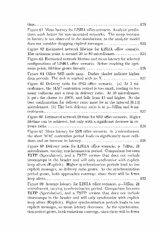
Figure 61 Mean latency for LISHA o�ce scenario. Analytic predic-tions work better for non-saturated networks. The steep increasein latency is not observed in the simulations, as the analytic modeldoes not consider dropping expired messages. . . . . . . . . . . . . . . . . . . . . . 123

Figure 62 Estimated network lifetime for LISHA o�ce scenario.The optimum point is around 50 to 80 microframes. . . . . . . . . . . . . . . 124

Figure 63 Estimated network lifetime and mean latency for selectedcon�gurations of LISHA o�ce scenario. Before reaching the opti-mum point, lifetime grows linearly. . . . . . . . . . . . . . . . . . . . . . . . . . . . . . . . 125

Figure 64 O�ce SSB node map. Darker shades indicate higherdata periods. The sink is marked with an X. . . . . . . . . . . . . . . . . . . . . . 127

Figure 65 Delivery ratio for SSB o�ce scenario. (a) At 5 mi-croframes, the MAC contention period is too small, leading to toomany collisions and a drop in delivery ratio. At 10 microframes,it gets the closest to 100%, and falls from 15 and higher. So thebest con�guration for delivery ratio must be in the interval [6,14]microframes. (b) The best delivery ratio is at p=7dBm and 6 mi-croframes. . . . . . . . . . . . . . . . . . . . . . . . . . . . . . . . . . . . . . . . . . . . . . . . . . . . . . . . . 127

Figure 66 Estimated network lifetime for SSB o�ce scenario. Higherlifetime can be achieved, but only with a signi�cant decrease in de-livery ratio. . . . . . . . . . . . . . . . . . . . . . . . . . . . . . . . . . . . . . . . . . . . . . . . . . . . . . . 128

Figure 67 Mean latency for SSB o�ce scenario. At 5 microframes,the short MAC contention period leads to signi�cantly more colli-sions and an increase in latency. . . . . . . . . . . . . . . . . . . . . . . . . . . . . . . . . . . 128

Figure 68 Delivery ratio for LISHA o�ce scenario, p=7dBm, 21microframes, varying synchronization period. Comparison betweenTSTP (Speculative), and a TSTP version that does not includetimestamps in the header and will only synchronize with explicitkeep alives (Explicit). Higher synchronization periods lead to lessexplicit messages, so delivery ratio grows. As the synchronizationperiod grows, both approaches converge, since there will be fewerkeep alives. . . . . . . . . . . . . . . . . . . . . . . . . . . . . . . . . . . . . . . . . . . . . . . . . . . . . . . . 132

Figure 69 Average latency for LISHA o�ce scenario, p=7dBm, 21microframes, varying synchronization period. Comparison betweenTSTP (Speculative), and a TSTP version that does not includetimestamps in the header and will only synchronize with explicitkeep alives (Explicit). Higher synchronization periods leads to lessexplicit messages, so mean latency decreases. As the synchroniza-tion period grows, both variations converge, since there will be fewer

keep alives. . . . . . . . . . . . . . . . . . . . . . . . . . . . . . . . . . . . . . . . . . . . . . . . . . . . . . . . 133

Figure 70 Number of explicit synchronization messages for LISHAo�ce scenario. �Theoretical� is one keep alive per node per syn-chronization half period. �Explicit� sends more keep alives due toimperfect channel conditions. �Speculative� sends less because ituses regular data messages as synchronization messages most ofthe time. At periods greater than 140s, Speculative reaches zeroexplicit synchronization messages. . . . . . . . . . . . . . . . . . . . . . . . . . . . . . . . . 134

Figure 71 Average clock error for LISHA o�ce scenario. Clock errorshould be inversely proportional to synchronization period. How-ever, as the synchronization period grows, delivery ratio also grows,and this indicates that nodes are able to access more synchroniza-tion messages more often, so clock error is actually lower at highersynchronization periods. For periods >160s (for Speculative) and>200s (for Explicit), delivery ratio stabilizes and clock error growsaccording to the sync period. . . . . . . . . . . . . . . . . . . . . . . . . . . . . . . . . . . . . . 136

Figure 72 Energy consumption compared to theoretical explicit ap-proach for LISHA o�ce scenario. Theoretical energy gain is calcu-lated comparing the cost of including timestamps in every messageto the savings in number of explicit synchronization messages. . . . . 137

Figure 73 Estimated network lifetime for LISHA o�ce scenario.The Speculative approach saves energy signi�catively. . . . . . . . . . . . . 138

Figure 74 Delivery ratio for SSB o�ce scenario, with p=7dBm and6 microframes. Similarly to the LISHA variation, delivery ratiogrows as less synchronization messages are generated. . . . . . . . . . . . . 138

Figure 75 Average latency for SSB o�ce scenario. Similarly to theLISHA variation, latency decreases as less synchronization messagesare generated. . . . . . . . . . . . . . . . . . . . . . . . . . . . . . . . . . . . . . . . . . . . . . . . . . . . . 139

Figure 76 Number of explicit synchronization messages for SSBo�ce scenario. �Theoretical� is one keep alive per node per halfsynchronization period. �Explicit� sends more keep alives due toimperfect channel conditions. �Speculative� sends less because ituses regular data messages as synchronization messages most ofthe time. At periods greater than 140s, Speculative reaches zeroexplicit synchronization messages. . . . . . . . . . . . . . . . . . . . . . . . . . . . . . . . . 140

Figure 77 Average clock error for SSB o�ce scenario. Clock errorshould be inversely proportional to synchronization period. How-ever, as the synchronization period grows, delivery ratio also grows,and this indicates that nodes are able to access more synchroniza-tion messages more often, so clock error is actually lower at higher

synchronization periods. . . . . . . . . . . . . . . . . . . . . . . . . . . . . . . . . . . . . . . . . . . 141

Figure 78 Energy consumption compared to theoretical explicit ap-proach for SSB o�ce scenario. Theoretical energy gain is calculatedcomparing the cost of including timestamps in every message tothe savings in number of explicit synchronization messages. Thetheoretical approach quickly outperforms the speculative, which isstill better than �Explicit�, an implementation of the theoreticalapproach measured under the same conditions as �Speculative�. . . . 142

Figure 79 Estimated network lifetime for SSB o�ce scenario. Bothapproaches show similar results. . . . . . . . . . . . . . . . . . . . . . . . . . . . . . . . . . . 143

Figure 80 Number of explicit synchronization messages for envi-ronment monitoring scenario, p=7dBm, d=60s. �Theoretical� isone keep alive per node per half synchronization period. �Explicit�sends more keep alives due to imperfect channel conditions. �Spec-ulative� sends less because it uses regular data messages as synchro-nization messages most of the time. . . . . . . . . . . . . . . . . . . . . . . . . . . . . . . 145

Figure 81 Number of explicit synchronization messages for environ-ment monitoring scenario, p=7dBm, d=600s. . . . . . . . . . . . . . . . . . . . . . 145

Figure 82 Average latency for environment monitoring scenario,d=60s. Only at synchronization periods of 300s the Explicit ap-proach reaches a slightly better average. . . . . . . . . . . . . . . . . . . . . . . . . . . 146

Figure 83 Average latency for environment monitoring scenario,d=600s. Only at synchronization periods of 3600s the Explicit ap-proach reaches a slightly better average. . . . . . . . . . . . . . . . . . . . . . . . . . . 146

Figure 84 Average clock error for environment monitoring scenario,d=60s. . . . . . . . . . . . . . . . . . . . . . . . . . . . . . . . . . . . . . . . . . . . . . . . . . . . . . . . . . . . 147

Figure 85 Average clock error for environment monitoring scenario,d=600s. . . . . . . . . . . . . . . . . . . . . . . . . . . . . . . . . . . . . . . . . . . . . . . . . . . . . . . . . . . 148

Figure 86 Energy consumption compared to theoretical explicit ap-proach for environment monitoring scenario, d=60s. . . . . . . . . . . . . . . 148

Figure 87 Energy consumption compared to theoretical explicit ap-proach for environment monitoring scenario, d=600s. . . . . . . . . . . . . . 149

Figure 88 Estimated network lifetime for environment monitoringscenario, d=60s. Only at synchronization periods of 300s the Ex-plicit approach reaches a slightly better average. . . . . . . . . . . . . . . . . . . 150

Figure 89 Estimated network lifetime for environment monitoringscenario, d=600s. Only at synchronization periods of 3600s theExplicit approach reaches a slightly better average. . . . . . . . . . . . . . . . 151

Figure 90 Estimated network lifetime and mean latency for SSB

o�ce scenario under di�erent routing metrics. . . . . . . . . . . . . . . . . . . . . 154

Figure 91 Fairness index and o�set standard deviation for SSB of-�ce scenario under di�erent routing metrics. . . . . . . . . . . . . . . . . . . . . . . 155

Figure 92 Estimated network lifetime and mean latency for environ-ment monitoring scenario, d=60s, under di�erent routing metrics. 155

Figure 93 Fairness index and o�set standard deviation for environ-ment monitoring scenario, d=60s, under di�erent routing metrics. 156

Figure 94 Estimated network lifetime and mean latency for environ-ment monitoring scenario, d=600s, under di�erent routing metrics.156

Figure 95 Fairness index and o�set standard deviation for environ-ment monitoring scenario, d=600s, under di�erent routing metrics.157

Figure 96 Average latency for environment monitoring scenario,d=300s. . . . . . . . . . . . . . . . . . . . . . . . . . . . . . . . . . . . . . . . . . . . . . . . . . . . . . . . . . . 177

Figure 97 Number of explicit synchronization messages for environ-ment monitoring scenario, d=300s. . . . . . . . . . . . . . . . . . . . . . . . . . . . . . . . 178

Figure 98 Average clock error for environment monitoring scenario,d=300s. . . . . . . . . . . . . . . . . . . . . . . . . . . . . . . . . . . . . . . . . . . . . . . . . . . . . . . . . . . 178

Figure 99 Energy consumption compared to theoretical explicit ap-proach for environment monitoring scenario, d=300s. . . . . . . . . . . . . . 179

Figure 100Estimated network lifetime for environment monitoringscenario, d=300s.. . . . . . . . . . . . . . . . . . . . . . . . . . . . . . . . . . . . . . . . . . . . . . . . . 179

Figure 101Average latency for environment monitoring scenario,d=900s. . . . . . . . . . . . . . . . . . . . . . . . . . . . . . . . . . . . . . . . . . . . . . . . . . . . . . . . . . . 180

Figure 102Number of explicit synchronization messages for environ-ment monitoring scenario, d=900s. . . . . . . . . . . . . . . . . . . . . . . . . . . . . . . . 180

Figure 103Average clock error for environment monitoring scenario,d=900s. . . . . . . . . . . . . . . . . . . . . . . . . . . . . . . . . . . . . . . . . . . . . . . . . . . . . . . . . . . 181

Figure 104Energy consumption compared to theoretical explicit ap-proach for environment monitoring scenario, d=900s. . . . . . . . . . . . . . 181

Figure 105Estimated network lifetime for environment monitoringscenario, d=900s.. . . . . . . . . . . . . . . . . . . . . . . . . . . . . . . . . . . . . . . . . . . . . . . . . 182

Figure 106Estimated network lifetime and mean latency for LISHAo�ce scenario under di�erent routing metrics. . . . . . . . . . . . . . . . . . . . . 183

Figure 107Fairness index and o�set standard deviation for LISHAo�ce scenario under di�erent routing metrics. . . . . . . . . . . . . . . . . . . . . 184

Figure 108Estimated network lifetime and mean latency for environ-ment monitoring scenario, d=300s, under di�erent routing metrics.184

Figure 109Fairness index and o�set standard deviation for environ-

ment monitoring scenario, d=300s, under di�erent routing metrics.185

Figure 110Estimated network lifetime and mean latency for environ-ment monitoring scenario, d=900s, under di�erent routing metrics.185

Figure 111Fairness index and o�set standard deviation for environ-ment monitoring scenario, d=900s, under di�erent routing metrics.186

List of Tables

Table 1 Main bu�er metadata used by TSTP. . . . . . . . . . . . . . . . . . . . 66

Table 2 Spatial scaling codes. . . . . . . . . . . . . . . . . . . . . . . . . . . . . . . . . . . . 72

Table 3 TSTP message types. . . . . . . . . . . . . . . . . . . . . . . . . . . . . . . . . . . . 72

Table 4 TSTP Interest modes. . . . . . . . . . . . . . . . . . . . . . . . . . . . . . . . . . . 73

Table 5 TSTP Control subtypes. . . . . . . . . . . . . . . . . . . . . . . . . . . . . . . . . 74

Table 6 Code size (bytes) for TSTP components and other proto-cols.. . . . . . . . . . . . . . . . . . . . . . . . . . . . . . . . . . . . . . . . . . . . . . . . . . . . . . . . . . . . . . 100

Table 7 Assessment of time overhead for bu�er management. . . . . 101

Table 8 Analytic model parameters. . . . . . . . . . . . . . . . . . . . . . . . . . . . . . 106

Table 9 Con�gurations for environment monitoring scenario. . . . . 112

Table 10 Selected con�gurations for each environment monitoringscenario. . . . . . . . . . . . . . . . . . . . . . . . . . . . . . . . . . . . . . . . . . . . . . . . . . . . . . . . . . 120

Table 11 Con�gurations for LISHA o�ce scenario. . . . . . . . . . . . . . . . 121

Table 12 Con�gurations for SSB o�ce scenario. . . . . . . . . . . . . . . . . . . 126

Table 13 Selected con�gurations for each o�ce scenario. . . . . . . . . . . 129

Contents

1 INTRODUCTION . . . . . . . . . . . . . . . . . . . . . . . . . . . . . 311.1 BACKGROUND . . . . . . . . . . . . . . . . . . . . . . . . . . . . . . . . . . . . 311.2 PREVIOUS RELATED WORK BY THE GROUP . . . . . . 341.3 OBJECTIVES . . . . . . . . . . . . . . . . . . . . . . . . . . . . . . . . . . . . . . 351.4 METHODOLOGY . . . . . . . . . . . . . . . . . . . . . . . . . . . . . . . . . . 361.5 OVERVIEW . . . . . . . . . . . . . . . . . . . . . . . . . . . . . . . . . . . . . . . . 362 TSTP DESIGN . . . . . . . . . . . . . . . . . . . . . . . . . . . . . . . . 392.1 PRINCIPLES . . . . . . . . . . . . . . . . . . . . . . . . . . . . . . . . . . . . . . . 392.1.1 Application Scenario . . . . . . . . . . . . . . . . . . . . . . . . . . . . . . 412.2 ARCHITECTURE . . . . . . . . . . . . . . . . . . . . . . . . . . . . . . . . . . 412.3 POSITION ESTIMATION . . . . . . . . . . . . . . . . . . . . . . . . . . . 432.4 TIME SYNCHRONIZATION . . . . . . . . . . . . . . . . . . . . . . . . . 442.5 MAC AND ROUTING . . . . . . . . . . . . . . . . . . . . . . . . . . . . . . . 492.5.1 Spatial Distortion . . . . . . . . . . . . . . . . . . . . . . . . . . . . . . . . . 532.5.2 TSTP Greedy Forwarding Algorithm . . . . . . . . . . . . . 542.6 SECURITY . . . . . . . . . . . . . . . . . . . . . . . . . . . . . . . . . . . . . . . . 562.7 SMARTDATA . . . . . . . . . . . . . . . . . . . . . . . . . . . . . . . . . . . . . . 593 TSTP IMPLEMENTATION . . . . . . . . . . . . . . . . . . . . 613.1 COMPONENT MODEL . . . . . . . . . . . . . . . . . . . . . . . . . . . . . 613.1.1 Zero-copy Bu�ers . . . . . . . . . . . . . . . . . . . . . . . . . . . . . . . . . 633.1.2 Metadata . . . . . . . . . . . . . . . . . . . . . . . . . . . . . . . . . . . . . . . . . 643.1.3 Event Propagation . . . . . . . . . . . . . . . . . . . . . . . . . . . . . . . . 653.1.4 Active Components . . . . . . . . . . . . . . . . . . . . . . . . . . . . . . . 673.1.5 Bootstrapping . . . . . . . . . . . . . . . . . . . . . . . . . . . . . . . . . . . . . 703.1.6 Interaction with the API Component . . . . . . . . . . . . . 703.2 COMMON MESSAGE FORMATS . . . . . . . . . . . . . . . . . . . . 713.3 POSITION ESTIMATION . . . . . . . . . . . . . . . . . . . . . . . . . . . 753.4 TIME SYNCHRONIZATION . . . . . . . . . . . . . . . . . . . . . . . . . 773.4.1 Sources of Synchronization Imprecision . . . . . . . . . . . 783.4.2 SPTP Implementation . . . . . . . . . . . . . . . . . . . . . . . . . . . . 803.5 MAC AND ROUTING . . . . . . . . . . . . . . . . . . . . . . . . . . . . . . . 803.5.1 Collisions and Hidden Nodes . . . . . . . . . . . . . . . . . . . . . . 843.6 SECURITY . . . . . . . . . . . . . . . . . . . . . . . . . . . . . . . . . . . . . . . . 913.6.1 Key establishment and management . . . . . . . . . . . . . . 913.7 SMARTDATA . . . . . . . . . . . . . . . . . . . . . . . . . . . . . . . . . . . . . . 944 TSTP EVALUATION . . . . . . . . . . . . . . . . . . . . . . . . . . 954.1 TOOLS AND DEBUGGING . . . . . . . . . . . . . . . . . . . . . . . . . 95

4.1.1 MAC State Machine Veri�cation . . . . . . . . . . . . . . . . . . 954.1.2 Security Library Veri�cation . . . . . . . . . . . . . . . . . . . . . . 964.1.3 Network Tra�c Visualization . . . . . . . . . . . . . . . . . . . . . 974.1.4 Simulation Execution . . . . . . . . . . . . . . . . . . . . . . . . . . . . . 974.2 EPOSMOTE III EXPERIMENTS . . . . . . . . . . . . . . . . . . . . . 994.2.1 Code Size . . . . . . . . . . . . . . . . . . . . . . . . . . . . . . . . . . . . . . . . . 994.2.2 Bu�er Management . . . . . . . . . . . . . . . . . . . . . . . . . . . . . . . 1004.2.2.1 Integrity Control . . . . . . . . . . . . . . . . . . . . . . . . . . . . . . . . . . . . 1014.2.3 Time Synchronization . . . . . . . . . . . . . . . . . . . . . . . . . . . . . 1014.3 ANALYTIC MODEL . . . . . . . . . . . . . . . . . . . . . . . . . . . . . . . . 1064.3.1 Limitations . . . . . . . . . . . . . . . . . . . . . . . . . . . . . . . . . . . . . . . 1084.4 SIMULATION EXPERIMENTS . . . . . . . . . . . . . . . . . . . . . . 1084.4.1 Sources of Random Variation . . . . . . . . . . . . . . . . . . . . . 1094.4.2 MAC Con�guration . . . . . . . . . . . . . . . . . . . . . . . . . . . . . . . 1104.4.2.1 Environment Monitoring Scenario . . . . . . . . . . . . . . . . . . . . . 1124.4.2.2 LISHA O�ce Scenario . . . . . . . . . . . . . . . . . . . . . . . . . . . . . . . 1204.4.2.3 SSB O�ce Scenario . . . . . . . . . . . . . . . . . . . . . . . . . . . . . . . . . . 1264.4.3 Synchronization . . . . . . . . . . . . . . . . . . . . . . . . . . . . . . . . . . . 1304.4.3.1 LISHA O�ce Scenario . . . . . . . . . . . . . . . . . . . . . . . . . . . . . . . 1314.4.3.2 SSB O�ce Scenario . . . . . . . . . . . . . . . . . . . . . . . . . . . . . . . . . . 1374.4.3.3 Environment Monitoring Scenario . . . . . . . . . . . . . . . . . . . . . 1444.4.4 Routing Metrics . . . . . . . . . . . . . . . . . . . . . . . . . . . . . . . . . . 1524.4.4.1 Expiry Metric . . . . . . . . . . . . . . . . . . . . . . . . . . . . . . . . . . . . . . . 1524.4.4.2 E�ort Metric . . . . . . . . . . . . . . . . . . . . . . . . . . . . . . . . . . . . . . . 1524.4.4.3 Evaluation . . . . . . . . . . . . . . . . . . . . . . . . . . . . . . . . . . . . . . . . . 1534.5 EVALUATION SUMMARY . . . . . . . . . . . . . . . . . . . . . . . . . . 1584.6 DISCUSSION . . . . . . . . . . . . . . . . . . . . . . . . . . . . . . . . . . . . . . . 1594.6.1 Possibilities for MAC improvements . . . . . . . . . . . . . . 1615 CONCLUSION . . . . . . . . . . . . . . . . . . . . . . . . . . . . . . . . 165

BIBLIOGRAPHY . . . . . . . . . . . . . . . . . . . . . . . . . . . . . 167APPENDIX A -- Additional simulation results . . . 177APPENDIX B -- Scienti�c Publications . . . . . . . . . . 189

31

1 INTRODUCTION

Wireless Sensor Networks (WSN) have been implemented inmany di�erent forms over the years. Buildings, homes, farms, rivers,the weather, assembly lines, and many more physical environments,can all be monitored and sometimes controlled by a wireless networkof cheap computing devices equipped with di�erent sensors and actua-tors. As these networks get connected to the Internet of Things (IoT),it is ever more important that they operate trustfully, with carefully-designed and -implemented domain-oriented Operating Systems andnetwork protocols. This work evaluates and improves the TrustfulSpace-Time Protocol (TSTP) (RESNER; FRÖHLICH, 2015a; RESNER;

ARAUJO; FRÖHLICH, 2017), taking it one step closer to its goal of beinga complete, e�cient solution for IoT-ready WSNs.

1.1 BACKGROUND

The concept of a network of cheap and small devices equippedwith a Microcontroller Unit (MCU), sensors, actuators, and wirelesscommunication hardware, is �tting to many application scenarios suchas building automation, environment monitoring, industrial coordina-tion, and several others. Usually these networks have at least onemaster node, called sink, towards which data gathered by sensor nodesis routed and ultimately delivered. When the network supports actu-ation, often the master node is also in charge of triggering commandmessages to actuators across the network.

Each application scenario has its own priorities in relation to net-work requirements. An unwatched network of battery-powered sensorsmonitoring temperature of a remote forest will generate sparse tra�c,but need to stay operative for a long period of time with a limited powersupply. An industrial assembly-line machine with di�erent coordinatedparts might need reliable and low-latency communication with precisetime synchronization, while having access to mains power supply. Anautomated o�ce room might need a more balanced energy/time re-lation, with some devices such as power-consumption-monitoring out-lets with access to mains power generating non-critical messages, whileother devices such as alarms or movement sensors are powered by bat-teries and sparsely generate important messages with a strong timerequirement. These issues bring optimization problems involving many

32

variables for the underlying communication protocol to solve for eachparticular network.

Such optimization problems are not the only challenges thatmodern WSNs need to consider. In the majority of applications, themost important concern about the network is the data collected. Theproduced data often need to be made available to agents outside thenetwork (such as domain-expert analysts or arti�cial intelligence) foranalysis, who will guide decisions about the physical system of interest,or prompt command messages that, from the perspective of the WSN,come from outside the network. A popular way of making the dataavailable to sophisticated and well-established pieces of software is toconnect the WSN to the Internet in some way. This can be done eitherby using a protocol stack such as TCP/IP to communicate with sensornodes directly, or by turning the sink into a gateway between the WSNand the external world � which often means the Internet. Now, devicesonce on isolated networks are part of the Internet of Things (IoT).

The IoT highlights challenges that were present in WSNs fromthe beginning, but that can be ignored to a degree in self-con�ned net-works and systems. Greater attention is brought to communicationsecurity. Messages need to be authenticated, with veri�able integrity,immune to replays, and sometimes con�dential. Data need to be uni-versally interpretable in terms of what is being measured, and whenand where each measurement was made. One must have evidence tobelieve that the data can be trusted. Enforcing the ful�llment of all ofthese additional requirements might take a prohibitive toll on the low-power WSN devices without careful and optimized Operating Systemand network protocol design and implementation.

There is a vast body of work in the literature to ful�ll each ofthese requirements. Several physical layers have been proposed, alongwith a myriad of medium access and routing protocols (HUANG et al.,2013; PATIL; BIRADAR, 2012). Such protocols have been made energy-aware (LONARE; WAHANE, 2013); aggregation and fusion strategieshave been employed (LEVIS et al., 2004); basic infrastructures have beenenriched with location (NIAN; SIVA; POELLABAUER, 2017), timing (DJE-NOURI; BAGAA, 2016), and security protocols (GRANJAL; MONTEIRO;

SILVA, 2015); operating systems have been designed to support higher-level abstractions (DIXON et al., 2012), along with large-scale manage-ment systems built to handle the produced data properly (HULBERT et

al., 2016). Extensive research is also being carried out on cross-layeroptimizations for WSN protocols (MENDES; RODRIGUES, 2011).

WSN applications often require many or all of these features. If

33

the needed functionality is not architecturally granted, often times lay-ers of heterogeneous, self-contained middleware are added. The addedsoftware comes with an integration cost and often results in unneces-sary replication of data. A cross-layer protocol design can eliminatethis overhead, save a large number of control messages, and improvedecision making within the protocol by pig-tailing control informationon ordinary data packets and subsequently organizing and sharing thatinformation with all protocol components.

Cross-layer designs are highly promising for WSN and wirelesscommunication protocols in general (FU et al., 2014). Duty-cycling pro-tocols at the Medium Access Control (MAC) level are constantly evolv-ing (HUANG et al., 2013), and even the earlier designs demonstratedthat devices could operate for a long time o� of a pair of AA bat-teries (POLASTRE; HILL; CULLER, 2004). Network lifetime can be in-creased even more with energy-aware routing algorithms (OKAZAKI;FRÖHLICH, 2012). Hardware implementations of symmetric-key secu-rity algorithms in WSN devices are getting commonplace due to theirwide adoption (e.g. AES being included in the IEEE 802.15.4 stan-dard (IEEE. . . , 2011)).

The Trustful Space-Time Protocol aims to be a complete commu-nication solution for WSN/IoT, combining all of these techniques andmore to fully contemplate the aforementioned requirements. TSTPis an application-oriented, cross-layer protocol for IoT-ready WSNsthat focuses on e�ciently providing functionality recurrently needed bysuch systems: trusted, timed, geo-referenced, SI-compliant data thatis resource-e�ciently delivered to a sink. TSTP grants these func-tionalities directly to the application in the form of a complete net-working entity, which allows the design of optimized, synergistic, tightcooperation of sub-protocols while eliminating the need for additionalheterogeneous software layers. TSTP integrates time synchronization,spatial localization, security, MAC, routing, and a data-centric API.The tightly-coupled design is mapped onto a low-overhead, modularimplementation, exploring template metaprogramming techniques toadapt and combine basic building blocks. An event-driven architecturethat makes use of zero-copy bu�ers and metadata is used to handlecrosscutting concerns.

In this work, TSTP's design is detailed with de�nitions of al-gorithms, sub-components, and message formats and usage. The im-plementation of TSTP for a real WSN device is presented in detail.This implementation is validated through controlled experiments, withanalysis and debug tools, and observation of di�erent real-world de-

34

ployments. The real-world analyses are complemented by simulationexperiments that investigate di�erent and larger-scale scenarios, as wellas more controlled evaluations of speci�c aspects. The analyses allow�ne-tuning and improvement of di�erent aspects of the protocol foreach scenario.

1.2 PREVIOUS RELATED WORK BY THE GROUP

This masters project was realized at the Software/Hardware In-tegration Laboratory (LISHA) at the Federal University of Santa Cata-rina (UFSC). Over the last decades, several research projects have beenconducted in the group under the supervision of professor Antônio Au-gusto Fröhlich in the topic of IoT and WSN protocols. The presentwork is built upon the research of many of these previous works. Theseworks granted the group the required perspective and experience whichled to the idea of the Trustful Space-Time Protocol. What follows is alist in chronological order of the main past contributions � with theirmain authors � that directly in�uenced the present work and ultimatelymade it possible.

• Gilles Pokam (1999): Pioneering work in static metaprogrammingframeworks applied to communication systems;

• Eduardo A. Billo (2002): Application of these techniques on theimplementation of a Bluetooth stack;

• Thiago R. C. Santos (2005): Implementation of a component-based communication framework, with bu�ers circulating fromone component to the next;

• Lucas F. Wanner (2006): Application of these techniques on animplementation for WSN devices running EPOS and equippedwith the CC1000 radio communication chip;

• Ricardo Reghelin (2006): Design and implementation of HECOPS,a decentralized location system for sensor networks using cooper-ative calibration and heuristics;

• Rafael P. Pires (2008): Evaluation of HECOPS;

• Lucas Torri (2008): Application of the IEEE 1451 standard onWSN devices running EPOS;

35

• Tiago R. Mück (2009): Design and implementation of a commu-nication framework for Software-De�ned Radio;

• Rodrigo V. Steiner (2010): Performance evaluation of C-MAC, aCon�gurable MAC framework, on EPOS;

• Alexandre M. Okazaki (2011): Application of energy-aware Ant-Colony Optimizations on routing protocols for WSNs;

• Peterson Oliveira (2012): Application of the Precision-Time Pro-tocol (PTP) on WSN devices running EPOS.

The author would also like to acknowledge the following peopleand (some of) their direct contributions to the present work:

• Antônio A. Fröhlich: For the idea and high-level design of TSTP,as well as the direct work in every step of TSTP's conception,design, implementation, and documentation;

• Gustavo M. Araujo: For the work and guidance on the initialport of TSTP for the OMNeT++ simulator and the Castaliaframework;

• Jean E. Martina: For the expert guidance in the security aspectsof the protocol;

• Sérgio A. Soares: For the fruitful early discussions and work onthe concrete protocol-level design of TSTP.

1.3 OBJECTIVES

The main goal of this work is to evaluate the performance of theTrustful Space-Time Protocol. This is done by achieving the followingspeci�c objectives:

• Implement TSTP for WSN hardware and a WSN simulator. Theimplementation choices will be documented, with descriptions oftechniques, algorithms, and message formats. It should be ad-equate to control real-world physical environments with sensorsand actuators, and make the generated data available to higher-level applications;

• Perform experiments to analyze various aspects of the implemen-tations. The protocol's behavior in terms of synchronization ac-curacy, latency, and energy consumption will be characterized for

36

di�erent application scenarios. Implementation overhead will bemeasured to justify the employed techniques;

• Optimize parameters and propose changes to improve the proto-col for each particular scenario based on the results of the analy-ses.

1.4 METHODOLOGY

TSTP is implemented in two platforms. For most of the perfor-mance evaluations, the OMNeT++ (OPENSIM, 2017) network simulatorwith the Castalia (BOULIS, 2017) framework is used. For real-world ap-plications and evaluation, TSTP is also implemented on the EmbeddedParallel Operating System (EPOS), for the EPOSMote III platform.By the time of this writing, several TSTP networks are using this lat-ter implementation for di�erent applications: a smart room at LISHA;a smart room at UFSC's Smart Solar Building (SSB); and a networkof hydrologic monitoring stations deployed near UFSC. The use of theprotocol in real-world networks helps �nd problems in the implemen-tation, as well as validate the adequacy of the protocol's features. Allthe data produced by TSTP nodes is encapsulated with the SmartDataAPI and stored at UFSC's IoT servers (LISHA, 2017).

1.5 OVERVIEW

Chapter 2 presents in detail the cross-layer design of the Trust-ful Space-Time Protocol. TSTP de�nes a novel way of thinking andprogramming WSN: instead of focusing on speci�c devices with id-iosyncratic sensor/actuator hardware, TSTP proposes to think aboutspace-time regions with geographic characteristics represented by unitsof the International System (SI). Devices in those regions might providethe ability to sense these characteristics and/or modify them. Space-time coordinates are used as network addresses for each device, andtherefore algorithms for synchronizing space and time are included inthe protocol. Messages are routed geographically as a result of an in-teraction between a Router and a low-power Medium Access Control(MAC) component. Security aspects of the protocol are also presentedin this chapter.

Chapter 3 shows that the tight interactions between TSTP'scross-layer subcomponents do not have to result in a tightly-coupled,

37

monolithic, or overhead-heavy implementation. This chapter brings adetailed presentation of the component-based implementation that ex-plores template metaprogramming techniques to adapt and combinebasic building blocks. An event-driven, subscription-based architec-ture that makes use of zero-copy, metadata-enriched bu�ers is used tohandle crosscutting concerns.

In Chapter 4, several aspects of the protocol are evaluated usingdi�erent approaches. Experiments with real hardware are performedto evaluate the limits of time synchronization and the correctness ofthe MAC state machine implementation. Detailed investigations onthe impact of several parameters of the protocol are performed on asimulator. This chapter also analyzes the implementation overhead,both in terms of memory and execution time for signi�cative aspects.

The work is concluded in Chapter 5, with a recapitulation of themain contributions and �nal remarks.

39

2 TSTP DESIGN

Parts of this chapter appeared earlier in:

• Design Rationale of a Cross-layer, Trustful Space-Time Protocolfor Wireless Sensor Networks(RESNER; FRÖHLICH, 2015a)

• Speculative Precision Time Protocol: submicrosecond clock syn-chronization for the IoT(RESNER; FRÖHLICH; WANNER, 2016)

• TSTP MAC: A Foundation for the Trustful Space-Time Protocol(RESNER; FRÖHLICH, 2016)

• Design and Implementation of a Cross-Layer IoT Protocol(RESNER; ARAUJO; FRÖHLICH, 2017)

TSTP is composed of a suite of sub-protocols that are intimatelyintegrated in a cross-layer architecture ranging from the Medium AccessControl layer to the Application layer. This chapter presents the maininsights behind the concept of TSTP. Later, several aspects of protocoldesign are explored for the architecture as a whole and speci�cally foreach of the sub-protocols.

2.1 PRINCIPLES

In general, to fully describe the relevant characteristics of a mea-surement by a sensor, one needs to at least determine precisely whereand when the measurement happened, and what is the quantity be-ing measured. This information might come indirectly, such as �sen-sor ABC3217, with address 1.2.3.4, reported the value 0x1234 as its145th measurement.� One would then look at some table to �gure outwhere that device with that address is located and when did its 145th

measurement happen, then lookup the datasheet of sensor ABC3217 todetermine what 0x1234 means. Most infrastructures will re�ne andtranslate this information automatically along its way from measure-ment to delivery at the sink to storage to display, and �nally presentuseful information to the end user.

TSTP proposes to express information from the beginning interms that make sense in the real world. Every TSTP device is aware

40

of its spatial location, has access to a common source of time, and isaware of what physical quantities it is working with. A measurementfrom a TSTP device would be, at any point, directly interpretable as�a sensor at coordinates 27◦36'01.5�S 48◦31'06.4�W reported the value42kg at December 1st 2017, 14:32:01 GMT�. Unix time presents a well-de�ned and simple way of representing time. Coordinate systems suchas Earth-Centered, Earth-Fixed (ECEF) allow a common representa-tion of space as a triple of coordinates in relation to the center of theEarth. The International System (SI) of units de�nes a codi�able wayof representing physical quantities.

Another major design principle of TSTP is to avoid unnecessaryreplication of information across the infrastructure. Instead of de�ninglogical addresses to locate devices in the network, TSTP uses Space-Time itself as a network address. This concept might not be applicableto networks in general, but in most cases it is natural to WSNs. Ul-timately, one does not want to know �what value is sensor 1.2.3.4

measuring�, but rather �what is the temperature over there now�. Adirect addressing by space and time allows the network to naturallyroute messages geographically, and to eventually detect and drop ex-pired ones. In this context, traditional network addresses are simplyan indirect way of representing space.

To further reduce unnecessary replication of information, TSTPleverages the broadcast nature of wireless media to allow nodes to peekat passing tra�c and speculatively make decisions: when necessary,nodes will look at timestamps and coordinates in TSTP messages topassively synchronize their clocks and location. They might canceltheir transmissions by detecting that other nodes transmitted equiva-lent messages.

As TSTP shifts the focus away from particular sensor nodes andtowards data, it becomes even more important to architecturally pro-vide the basis for trusting the data. TSTP nodes are able to signtheir messages, so that they have veri�able authenticity, integrity, andtiming. Nodes are made aware of their sensor hardware accuracy andtiming limits, so that they will only respond to data requests whenthese parameters match. On the advent of aging, broken, or mali-cious sensors, TSTP provides architectural support for neighbors of anuntrustworthy node to speculatively detect a mismatch between whatthat node says a physical quantity is and what their own sensors aremeasuring.

To provide a common notion of Space-Time and ful�ll the re-quirements of an IoT-ready WSN, TSTP includes algorithms for spa-

41

tial localization, time synchronization, Medium Access Control (MAC),power management, routing, and security.

2.1.1 Application Scenario

TSTP primarily supports ad-hoc, multihop networks of wirelessdevices in which most of the tra�c is delivered to a single destination(all-to-sink). Network addresses are replaced by spatial coordinates,such that it bene�ts applications concerned more with gathering datafrom a physical environment than with addressing particular networkdevices. Examples of such applications are:

1. A network of battery-powered devices periodically gathering tem-perature information from a large open �eld;

2. A room automation system with network-enabled devices attachedto lamps, outlets, and other sensors and actuators, measuringpower consumption and controlling it by commanding lights andair conditioning units;

3. An alarm system with di�erent sensors to detect physical intru-sion in a region, �ring alarms when it does.

TSTP is not aimed towards a range of more traditional Internetapplications. For example:

1. Applications that handle non-spatial-sensitive data, such as generic�le storage services;

2. Applications that handle one-to-many or many-to-many tra�c ofdata, such as video streaming or group messaging;

3. Structured networks mostly concerned with granting high through-put, such as Internet backbone infrastructure.

2.2 ARCHITECTURE

TSTP is designed as a collaboration of 6 protocol componentsthat interact with each other: MAC, Router, Timekeeper, Locator,Security, and API. The Timekeeper is responsible for precise clock

42

synchronization across the network. It currently implements the Spec-ulative Precision Time Protocol (SPTP) (Section 2.4), but any high-precision protocol could be used. The Locator is responsible for keep-ing spatial coordinates up to date, particularly in nodes devoid of a GPSreceiver or for which a static location was not de�ned at deployment-time. It currently implements the Heuristic Cooperative CalibrationPositioning System (HECOPS) (Section 2.3). The Router imple-ments a greedy, fully-reactive, geographic routing strategy as it decideswhen to forward messages from other nodes and implements metricsfor relay selection used by the MAC (Section 2.5). Security is re-sponsible for encrypting and/or signing messages, as well as managingcryptographic keys (Section 2.6). The MAC component manages thenetwork interface and communication channel, sending and receivingnetwork packets containing TSTP messages (Section 2.5). The APIhandles interactions between the applications and the network throughthe protocol (Section 2.7).

Unlike traditional layered architectures, components are designedto interact with one-another to achieve high performance. For example,MAC and Timekeeper collaborate to leverage the low-level synchroniza-tion process necessary for demodulation of radio signals, achieving high-precision timestamping and clock synchronization. MAC and Routercollaborate to de�ne and apply metrics to select winners in channelaccess contention. Locator and Timekeeper help Security assess thevalidity of messages and implement sophisticated time-aware securitymechanisms.

To avoid tightly-coupled interactions between component imple-mentations, TSTP employs a vertical data exchange plane model (FUet al., 2014), orderly delivering metadata-enriched zero-copy networkbu�ers to each component, as illustrated in Figure 1. Componentsshare information with each other either by means of metadata at-tached to each bu�er (which is not transmitted through the network),or the TSTP message itself (which may be transmitted through thenetwork) contained in the same bu�er. Bu�ers are further explained inSection 3.1.1.

To prevent replication of information in TSTP messages, insteadof con�ning each component to its own speci�c header of a message,the full message contained in a bu�er is accessible to any component.This way, if more than one component need timing control for mes-sages (e.g. Timekeeper and API), for example, they can all use thesame time �elds, rather than potentially including the same informa-tion (directly or indirectly) more than once. To enable routing and

43

Router Timekeeper

MAC

LocatorSecurity

Buffer

Message

MetadataControl

API Radio

Figure 1: TSTP component interactions and Bu�er life-cycle.

passive synchronization, the TSTP common message header includesinformation about the node that is currently transmitting that mes-sage, such as its coordinates and the precise transmission time. TheTSTP header is fully presented in Section 3.2.

2.3 POSITION ESTIMATION

The Global Positioning System (GPS) has become the de factostandard for automatic device localization. Although it is a reliablesolution for outdoor environments, nodes operating indoors generallycan't bene�t from it, and adding GPS receivers to a WSN node in-curs additional energy and �nancial costs. In mobile wireless networks,there are several algorithms that allow nodes to estimate their locationwith no additional hardware, leveraging characteristics of particularradio signaling technology, such as the Received Signal Strength Indi-cation (RSSI) provided by an IEEE 802.15.4 implementation (PIRES;WANNER; FRÖHLICH, 2008), or the Time Di�erence of Arrival (TDOA)provided by a UWB transceiver (OLIVEIRA et al., 2012).

Given that nodes can estimate their distances to one anotherbased on physical layer characteristics and there are anchor nodes inthe network that know their own position, there are many techniquesto determine the position of a given node, such as trilateration andmin-max (NIAN; SIVA; POELLABAUER, 2017). The location of anchornodes can be determined equipping a subset of the nodes with GPSreceivers, or simply pre-set if a node is not mobile. This makes anchornodes more expensive and/or di�cult to deploy, thus it is generallydesirable to reduce their number.

Regardless of the chosen position estimation algorithm, it willcome with a precision limitation. The Heuristic Environmental Con-

44

sideration Over Positioning System (HECOPS) (REGHELIN; FRÖHLICH,2006) enriches the localization strategy by establishing a ranking sys-tem to determine the reliability of each estimated position. It usesheuristics to mitigate the e�ects of measurement errors (which can behigh, especially in low-cost nodes). Such enrichments reduce the num-ber of necessary anchor nodes by allowing non-anchor nodes to act asanchors when their con�dence is high enough.

The original implementation of HECOPS uses RSSI values onIEEE 802.15.4 devices. Nodes maintain a table of neighbor data con-taining their alleged coordinates, con�dence, and RSSI-based distancemeasurements. Every node periodically broadcasts its table, and thenodes receiving it can update theirs. With enough data from neighbors,a node n can estimate its position and its con�dence Cn via trilatera-tion.

To cope with the irregular nature of RF signals and RSSI (orany other) measurements, HECOPS de�nes a deviation heuristic value,which is obtained when two anchor nodes estimate their distance toeach other via RSSI and then compare it to their actual distance (sincetheir coordinates are known). When a deviation is detected betweennodes A and B, it is heuristically assumed to a�ect every node in thetriangular area tri(A,B), illustrated in Figure 2.

A node's con�dence in its location is determined by Equation 2.1,selecting the 3 reference nodes in its table with the best con�dence.

Cn =

∑3i=1(Ci × 0.75 + Ctri(i,n) × 0.25)

3× 0.8 (2.1)

In TSTP, non-anchor nodes build their position estimation ta-bles simply by observing the TSTP header of passing messages, whichcontain the coordinates and con�dence of the transmitting node. Theimplementation of HECOPS in TSTP, realized by the Locator compo-nent, is presented in Section 3.3.

2.4 TIME SYNCHRONIZATION

Time in computing systems is typically kept by counting cyclesof a piezoelectric crystal oscillator. The frequency of oscillation is de-termined by the cut, vibration mode (longitudinal, transverse), and thesize of the crystal wafer (ZHOU et al., 2008). Imprecisions and defectsin the manufacturing process therefore lead to a deviation in oscilla-tion frequency across di�erent parts with the same nominal frequency.

45

We expect the required anchor proportion be as small

as possible, without compromising the results accuracy.

For that reason, the HECOPS allows nodes with estimated

positions to be chosen as landmarks. In order not to let

this characteristic compromise the system’s performance,

HECOPS uses a heuristic scheme that gives a value to the

confidence on location information given by nodes. Each

node, when calculating its position, defines a confidence

value on the result obtained. This value ranks the nodes

that should be chosen by a node that has to estimate its

location.

Confidence calculation is based on the confidence

value of the nodes chosen as landmarks and on the con-

fidence of the nodes used in distance calibration related to

that landmarks. In a scale varying from 0 to 1.0, anchor

nodes have maximum confidence on its position, equal to

1.0. The other nodes have confidence limited by 0.8, given

by equation 2, where Cx is the confidence on position that

is being calculated by a node X, Ci the confidence on each

landmark chosen by X (n in total) and Cix the confidence

of the node that, together with the node i, have defined the

deviation applied to the distance between the nodes i and

X, if any (In Figure 2, Cix would be the confidence on

node B, considering i the node A).

Cx = 0.8×

∑n

i=1(Ci × 0.75 + Cix × 0.25)

n(2)

Location information received from anchors is very

trustworthy. But, if the distance estimation of that node

has been calibrated by another node, the confidence is

even greater. For this reason, the weights of 0.75 and 0.25

were attributed for the confidence on a chosen landmark

and the confidence of the node used to calibrate the dis-

tance between them, respectively. Thus, when a node that

has to estimate its position has already chosen its land-

marks and have the estimated distances to all of them, it’s

enough to apply some method to calculate coordinates,

like lateration or min-max [6].

In the beginning, only anchor nodes know their posi-

tions. They start by broadcasting their identification (ID),

coordinates (x,y) and confidence values (Figure 3(a)). The

nodes that receive this message store the information to-

gether with the RSSI reading. If the receiving node al-

ready knows its position, it calculates the distance and de-

viation between itself and the sending node, and broad-

casts this information (Figure 3(b)). This information is

in turn stored by the nodes who wish estimate their posi-

tions.

ID

x y

Confidence

(a) Position information

message.

IDID BA

AB

ABdistance

deviation

(b) Deviation information

message.

Figure 3. Content of exchanged messages

d =

dev

RSSI

AC

AB

C

0.5 dA

C

B

dev AB

AB

Figure 4. Determining if two nodes are in the

same direction, in order to use calibration

When a message with deviation information is received

by a node that doesn’t know its coordinates, it checks if it’s

in the same direction than the transmitter, related to the

third node described in the message. If it is, it calibrates

the RSSI reading of a message sent by that third node with

the deviation.

The checking of a node to discover if it’s in the same

direction of another one related to a sending node is made

according to proximity between them. In Figure 4, the

node C receives a message from B about the deviation be-

tween A and B. So, node C verifies if its distance to node

B is lower than the half of the distance to A. In a positive

case, node C calibrates the RSSI reading of the last mes-

sage received from A with the deviation between A and B.

When these conditions are met, hereinafter we will refer

as the “tri” occurrence.

Position information messages are stored by the nodes

that will estimate its coordinates in a list ordered by the

confidence value. When the list size reaches 3 it’s already

possible to execute the position calculation. The 3 nodes

of the list with greatest confidence in their positions are

chosen as landmarks.

3. Simulations and Evaluation

In order to evaluate the location system implemented

in this work, and to allow tweaking of parameters in the

location algorithm, RSSI measurements were collected in

the field, and stored for offline execution. For this, a wrap-

per was developed to allow running the same code devel-

oped for the sensor platforms with EPOS [7], a deeply-

embedded operating system, and in UNIX workstations.

Through this wrapper, the same code that would run in

a sensor node runs in a thread, and message exchanging

is performed through memory copies, using the data col-

lected in the field.

In order to allow this execution scenario, RSSI mea-

surements were collected between every pair of nodes in

a 3× 3 sensor grid, with nodes 5m apart. These measure-

Figure 2: HECOPS deviation heuristic. A and B are anchor nodes thatdetect a deviation between them. C is inside the tri(A,B) area andcompensates for the deviation. Figure from (REGHELIN; FRÖHLICH,2006)

Furthermore, environmental factors such as temperature, aging, drivelevel, power supply noise, and vibration-induced noise also a�ect crystalstability and accuracy.

The accuracy of a crystal is its o�set from the target nominal fre-quency, while its stability is the spread of its frequency over time (ZHOUet al., 2008). Figure 3 shows examples for accuracy and stability sce-narios for crystal oscillators. Oscillators may be stable and accurate,stable but inaccurate, instable but accurate on the average, and insta-ble and inaccurate. Inaccuracy in frequency leads to the fact that twoindependent clocks, once synchronized, will drift apart without limit.Figure 4 shows the clock readings of di�erent EPOSMote III devicesdrifting apart over time1.

Improving stability and precision of clocks has been the target ofresearch and development, including Temperature-Compensated Crys-tal Oscillators (TCXO), Microcomputer-Compensated Crystal Oscilla-tors (MCXO), and Oven-Controlled Crystal Oscillators (OCXO), all ofwhich attempt to compensate for systematic and environmental vari-ations in oscillators (LEWIS, 1991). These mechanisms come at a costin terms of system volume, cost, and energy consumption. A com-plementary option is the employment of network time synchronizationprotocols.

Network time synchronization protocols typically work through

1Readings from CC2538's 32MHz timer with ±40ppm accuracy dedicated tonetwork software.

46

Time

Fre

quen

cy

Actual frequencyNominal Frequency

(a) Accurate and Stable

Time

Fre

quen

cy


(b) Inaccurate and Stable

Time

Fre

quen

cy


(c) Accurate and Unstable

Time

Fre

quen

cyActual frequencyNominal Frequency

(d) Inaccurate and Unstable

Figure 3: Accuracy and Stability of Crystal Oscillators

the exchange of timestamped messages between pairs of nodes (CRIS-TIAN, 1989). Each message typically contains a local timestamp of thesender. A series of messages are exchanged to estimate the time o�-set and drift between a pair of nodes (GUSELLA; ZATTI, 1989). Themost widely used protocol of this kind is the Network Time Proto-col (NTP) (MILLS, 1991). NTP targets Internet hosts and, due to itsmultihop nature, su�ers from constantly varying communication de-lays between hosts. Typical synchronization accuracy for NTP is onthe order of tens of milliseconds, making it unsuitable for time-criticalsensing and actuation applications.

In the wireless embedded sensing context, the Flooding TimeSynchronization Protocol (FTSP) (MARóTI et al., 2004) is the mostwidely cited time synchronization protocol. FTSP aims to synchro-nize an entire multihop network of wireless nodes to a single root node.The root node periodically broadcasts time synchronization messages,

47

0 100 200 300 400 500 600

−40

−20

020

40

Time (s)

Offs

et v

aria

tion

(us)

Figure 4: Clock drift of four di�erent EPOSMote III devices in relationto a �fth. One of the motes (in blue) diverged particularly quick in thisscenario.

each of which contains multiple timestamps. FTSP targets platformsusing radios with software-de�ned medium access control (MAC), andrelies on MAC-level timestamping combined with a characterization ofinterrupt handling timing. Each transmitted timestamp is acquired asclose to the physical send event as possible. This combination of pre-cise interrupt handling timing and multiple timestamps per messageallowed FTSP to achieve a 1-hop synchronization accuracy of ∼1.5 µs.

The introduction of the IEEE 1588 standard (IEEE, 2008), thePrecision Time Protocol (PTP), emphasized the need for high precision,sub-microsecond synchronization for distributed sensing and controlsystems (EIDSON, 2006). Compared to NTP, which uses application-level timestamping of network packets to account for drift and o�set,PTP can make use of advanced timestamping capabilities in the net-work interface hardware in order to reduce the temporal interferenceintroduced by various layers of software. PTP de�nes a hierarchy ofclocks, in which a grandmaster periodically broadcasts Sync messages,and other nodes send Delay Request messages which are replied byhigher clocks in the hierarchy, so that each node can measure with highaccuracy both network round-trip time and their own clock o�set.

48

cM(t1), cS(t'1)

Master Slave

cM(t1)

cM(t'2)

cS(t2)

cM(t'2)

sync

delay resp

delay req

Figure 5: Example of clock synchronization with PTP. cM (t1) andcM (t′2) are transmitted with the sync and delay resp messages, re-spectively.

To successfully synchronize in time, a node needs to estimate itsclock o�set and frequency drift in relation to a reference clock. Let Mdenote a master node with a reference clock and S a slave. Let cM (tm)represent the value of the timestamp counter of node M at physicaltime tm, and cS(t

′m) denote the value of the timestamp counter of

node S when it receives a message containing cM (tm). By collecting 4timestamps over the exchange of 3 messages, as illustrated in Figure 5,a slave node is able to estimate the round-trip time dTX according toEquation 2.2, and adjust its clock by subtracting the o�set φ given byEquation 2.3.

dTX =(cM (t′2)− cS(t2)) + (cS(t

′1)− cM (t1))

2(2.2)

φ = cS(t′1)− (cM (t1) + dTX) (2.3)

Once the o�set is corrected, node S is ready to estimate itsclock frequency drift in relation to M . After it receives a new messagecontaining cM (t3), the clock drift is given as:

fe =(cM (t3)− cS(t′3))− (cM (t2)− cS(t′2))

cM (t3)− cM (t2)(2.4)

The accuracy of this estimation is (SCHMID; DUTTA; SRIVASTAVA,

49

2010):

δQ =1

(t3 − t2) · fM(2.5)

where fM is the frequency of the clock of node M . The o�set anddrift estimation should be continually re-estimated, as clocks (especiallythe cheap clocks present in most WSN platforms) usually drift semi-randomly over time.

The set of equations presented allows synchronization even ifboth nodes are multiple hops away, and do not make assumptions aboutthe underlying network2. However, protocols such as FTSP require thatthe time dTX that timestamps take to travel from Master to Slave ispredictable with small enough jitter. If that is the case, calculatingclock o�sets become trivial, as Equation 2.3 can be applied simplyby observing one timestamp in the network. By observing a secondtimestamp, drift can be estimated according to Equation 2.4.

The Speculative Precision Time Protocol (SPTP), developed andused in the TSTP context, de�nes that synchronization happens hop-by-hop, and nodes synchronize their clocks with any other node that iscloser to the sink, which is the ultimate reference. By restricting syn-chronization to neighboring nodes, leveraging low-level timestampingby the MAC, and timestamping every message, SPTP estimates dTX

to high precision and allows nodes synchronize their clocks completelypassively, just by observing network tra�c, while keeping synchroniza-tion accuracy close to the maximum possible o�ered by the hardwareplatform. If a node is in a region with too sparse tra�c, it can generateKeep Alive messages, which carry only the TSTP header and prompta response from neighboring nodes to collect synchronization informa-tion. It can also set a Time Request bit on its messages to triggerresponses from neighbors. Figure 6 shows an example where node Asends a data message towards the sink, and synchronizes its clock tonode B while its message gets routed. SPTP's implementation is shownin Section 3.4.

2.5 MAC AND ROUTING

By including spatio-temporal data in every message, TSTP de-vices are able to localize themselves mostly passively, just by overhear-

2PTP allows �follow up� messages or low-level timestamping to improve synchro-nization accuracy, but these techniques do not change the fundamentals expressedin the equations.

50

A B

cB(t1)

cB(t1), cA(t'1)cB(t2)

m2

m1

C

cB(t2), cA(t'2)

m1

m1

m2

Figure 6: Example of clock synchronization between A and B withSPTP. Nodes to the right are closer to the sink. m1 and m2 are regulardata messages being routed towards the sink. m2 can also be triggeredby setting the Time Request bit in m1.

ing network tra�c. The overhearing of tra�c is possible because thewireless medium is inherently broadcast, such that any radio transmis-sion can be received by any listening device in a certain area3. Thisbroadcast nature brings problems of sender coordination: if more thanone transmission happens at the same time, they might collide anddestroy one another. Furthermore, radio hardware is relatively power-hungry in WSN devices, and much energy can be wasted by activeradios listening to the channel when there is no ongoing transmission,i.e. idle listening (POLASTRE; HILL; CULLER, 2004).

WSN protocols usually de�ne duty cycling techniques to mitigatethis problem: radios are turned on periodically to quickly check thechannel, and then turned o� if no activity is detected. This brings a tollon senders, however, since they do not know if there will be any receiverawake at all when they transmit their message. The classic solutionsto this problem are either synchronizing and scheduling transmissions,or sending long preambles (proportional to the sleep period) beforeeach message, to make sure that receivers will wake up at some pointduring the preamble and detect the transmission. Protocols adoptingthis latter solution are categorized as Preamble-Sampling MACs. Aperfect, global synchronization is generally a better approach, but very

3Calibrated with compatible frequency and demodulation parameters, and in alocation and moment where the transmitted signal can arrive with enough strengthand without too much destructive interference.

51

hard to achieve in practice, and can incur large overhead in terms ofcontrol messages. Preamble-sampling is generally much simpler, butmay impose large overhead in the transmission of any message.

B-MAC (POLASTRE; HILL; CULLER, 2004) is a well-known ex-ample of the Preamble-Sampling approach. Transmitters send a longcontinuous preamble and when a receiver detects it, the radio is kept onuntil reception of the data. In other protocols, such as MFP (BACHIRet al., 2006), the continuous preamble is divided into a series of smallframes, called microframes, containing a sequence number which servesas a countdown to the actual data transmission. This allows receiversto receive a single microframe, switch o� its radio during transmissionof the remaining microframes, and switch it on again just before thedata frame transmission.

In the Receiver-Based MAC (RB-MAC) (AKHAVAN; WATTEYNE;

AGHVAMI, 2011) protocol, senders transmit data without de�ning aMAC-layer destination. Preambles consist of microframes that containuseful information such as countdown to data transmission, sender dis-tance to sink and payload sequence number. All neighboring nodeswithin communication range of the sender sense the channel every Sinterval, obtain a microframe and extract the information; then, onlyeligible receivers (nodes closer to the �nal destination of the message)go back to sleep and wake up to receive the data at the time indicatedby the countdown. Nodes that receive the data without error are re-lay candidates, and start a contention timer based on its own distanceto the destination and possibly other factors (e.g. remaining energy),which when elapsed will trigger a CCA. The node with the shortestcontention time o�set will sense no channel activity and proceed totransmit the preamble for S units of time. Other relay candidates willdetect the winner's preamble containing the same sequence number,drop the data and go back to sleep since the packet is already beingforwarded. Figure 7 illustrates this process. As a consequence of theway relay candidates are determined, packets are geographically routedto the �nal destination in a greedy way.

RB-MAC is signi�cantly more resilient to lossy links when com-pared to sender-based MAC protocols (in which sender nodes keep theaddresses of perceived neighbors and de�ne a speci�c neighbor as re-ceiver for each message) (STEINER et al., 2013). As the number ofnetwork nodes increases, RB-MAC requires fewer retransmissions, con-sequently reducing latency and energy consumption (STEINER et al.,2013).

TSTP MAC is the component responsible for interfacing TSTP

52

Figure 7: Example of an RB-MAC message forwarding. Figure from(STEINER et al., 2013).

with the network with a special care for energy consumption. It cur-rently implements the mechanisms of RB-MAC. The contention o�setδ for a message m at any given node is locally calculated as:

δ(m) =R− (Dm −D)

R× S (2.6)

with D representing the current node's distance to the message's desti-nation, Dm representing the message sender's distance to the destina-tion, and R representing a network-wide parameter corresponding tothe radio range of the nodes. This equation makes nodes closer to thedestination wake up earlier, normalizes the o�set to the period S (sincenodes only route messages that come from nodes more distant to thedestination � as explained in Section 2.5.2, � it holds that D < Dm),and ensures that, if the destination is extremely far away, neighboringnodes (that are at the same discrete point in space in the scale of thetotal distance) will still have di�erent o�sets.

Messages being routed are kept on each involved node i in aqueue Qi. Each entry eQ in Qi represents a message m that is sched-uled for transmission or retransmission. In addition to the message, eQalso holdsm's Id (extracted from the microframes that preceded it), itsExpiry (extracted from its header), its destination Dst (either a previ-ously assigned sink or extracted from the payload), and the contentiono�set δ.

TSTP uses RB-MAC's implicit acknowledgment (ACK) to con-�rm the routing of messages. A node only removes a message from

53

its queue when it expires or when another message with the same Id

is overheard in the network (that is, when another node handles theforwarding of that message towards its destination). The only case inwhich an explicit ACK is used is when the message reaches its �naldestination: that node must retransmit the same message, just to ac-knowledge the last forwarder and any neighbors that might still havethat message queued. Since this last ACK has a Last Hop coordinateidentical to the destination, the calculated distance of zero won't bematched by any other node in the vicinity. The rest of this sectionconcerns routing aspects integrated in TSTP MAC. Further implemen-tation details of the MAC are exposed in Section 3.5.

2.5.1 Spatial Distortion

The default distance-based contention o�set δ, given by Equa-tion 2.6, can be made sensitive to other routing metrics according toapplication's needs. For example, it may take into account the re-maining battery charge or bu�er space of a node to ensure that nodesin an optimal path are not going to have their batteries depleted tooquickly (OKAZAKI; FRÖHLICH, 2012). To accomplish this, TSTP usesthe notion that those additional metrics distort space. A node run-ning out of memory or consuming too much energy can stretch space,increasing its distance to the destination so that other nodes in thevicinity become more likely to win the contention to retransmit a mes-sage. Conversely, a node transmitting a message that is close to ex-piring can shrink space, reducing its distance to the destination andthus increasing the chances of winning the contention and getting themessage transmitted earlier. Equation 2.7 rede�nes the o�set equationintroducing a distortion coe�cient α ∈ [0, 1]:

δ(m) = α× R− (Dm −D)

R× S (2.7)

The distortion coe�cient α de�nes how much other metrics in-�uence the perceived distance, and hence the o�set used for contention.It may take into account virtually any metric of interest, as long as itis a real number in the interval [0, 1]. A value of α < 1 decreases δ,increasing the node's likelihood of winning the contention, while α = 1takes into account only the node's distance to the destination.

54

2.5.2 TSTP Greedy Forwarding Algorithm

To prevent the distortion coe�cient from causing messages tobe forwarded to an incorrect destination, the TSTP Greedy Forward-ing Algorithm (Algorithm 1) ensures that all messages that a nodereceives and are queued for transmission satisfy the Progress Property:all messages relayed will make positive spatial progress towards thedestination. This property can be written as ∀j∀i{mji ∈ Qi|Di < Dj},meaning that each message mji from node j overheard by node i willbe stored in node i's transmission queue Qi if and only if the distanceDi from node i to the message's destination is smaller than the distanceDj from node j to the same destination.

Algorithm 1 TSTP Greedy Forwarding Algorithm

1: procedure GreedyForward(m)2: queued← false3: for each eQ ∈ Qi do

4: if m.id = eQ.id then

5: queued← true6: if Distance(m.LastHop,m.Dst) > Distance(Here,m.Dst)

then

7: delete m8: else

9: Qi.remove(eQ)10: delete m11: delete eQ12: end if

13: end if

14: end for

15: if queued = false then

16: if Distance(Here,m.Dst) > Distance(m.LastHop,m.Dst) then17: delete m18: else

19: Qi.insert(m)20: end if

21: end if

22: end procedure

Algorithm 1 handles four possible cases, illustrated in Figure 8:

Case 1 (lines 6, 7) : If a copy of the message m is already queuedand m is coming from a node farther from the destination, then

55

m is a retransmission attempt and can be ignored (the local copyremains on the queue for later retransmission).

Case 2 (lines 8, 9, 10, 11) : If a copy of m is already queued and mis coming from a node closer to the destination, then this meansthat the message has already made positive progress to the des-tination. The message m is therefore handled as an acknowledg-ment, causing the local copy eQ to be removed from Qi.

Case 3 (lines 16, 17) : If m is a new message but came from a nodecloser to the destination, then it means that this node (the re-ceiver) would not make positive progress towards the destination.The message is ignored.

Case 4 (lines 18, 19) : If m is a new message that came from anode more distant from the destination, then this node can makepositive progress towards the destination. It stores the messageon its queue and becomes a relay candidate for message m.

m1Qn

s dn

m1m2

(a) Case 1: n ignores m1, which wasalready in its transmission queue Qn.

m1m2

Qn

n ds

m1 m1

(b) Case 2: n deletes m1 from itsqueue, because s is closer to d.

m1m2

Qn

n ds

m3 m3

(c) Case 3: n ignores m3, because sis closer to d.

m3Qn

s dn

m1m2m3

(d) Case 4: n adds m3 to its queue,because n is closer to d than s is.

Figure 8: Possible cases for Algorithm 1. In each case, node s sends amessage with d as the destination, which is overheard by node n.

The following theorem proves that the Greedy Forwarding Algo-rithm ensures the Progress Property:

56

Theorem 1. The Greedy Forwarding Algorithm will store in queue Qi

any given incoming messages mji from node j overheard by node i ifand only if Di < Dj.

Proof. The proof is by contradiction. Suppose that ∃i,∃j,∃mji{mji ∈Qi|Di ≥ Dj} and that every Q is only altered by Algorithm 1. Themessage mji must have been included in Qi by Case 4 because it isthe only case that includes messages in the queue. But Case 4 onlyincludes a given messagemji in Qi ifDi < Dj , and since by assumptionDi ≥ Dj , it is not possible that mji was included in Qi by Case 4.Therefore, since Case 4 is the only case that could include mji in Qi,it must be true that mji 6∈ Qi, reaching a contradiction.

The theorem assumes that distances are expressed correctly. Dis-tances may be incorrect either by deliberate manipulation by a mali-cious node or by imprecision in the localization algorithm. For the �rstcase, since the router takes as parameter the average radio range Rof the network (Section 2.5), nodes drop messages that allegedly comefrom a distance greater than R. Besides preventing undesirable e�ectsof radio range asymmetry, this mechanism results in only nodes onehop away from the alleged source coordinates of the malicious mes-sage trying to forward it, and from that point on the message will berouted correctly. Regarding imprecisions in the localization algorithm,it may break the theorem at hops where nodes are so close that theirrelative positions are inverted. However, this will only ultimately routethe message to an incorrect destination if the locations of all nodes areconsistently and heavily skewed in the wrong direction, which is a veryunlikely situation. In both cases the message can take non-optimal hopstowards the destination, but will only be routed to an incorrect �naldestination if a large portion of the network is heavily compromised.

2.6 SECURITY

The fact that any properly con�gured radio interface can monitoror participate in WSN communications is very convenient for attack-ers. Generally, a secure WSN protocol must consider the principles ofcon�dentiality, authenticity and integrity (SUO et al., 2012). AES is ablock cipher that can enable these principles while being suitable tolow-power WSN devices. In fact, AES is a popular option in this do-main, being included in the IEEE 802.15.4 standard (IEEE. . . , 2011),

57

and many devices come with e�cient hardware-accelerated AES en-gines.

AES requires symmetric keys to be shared between the commu-nicating parties, and other strategies and/or algorithms are needed tosolve the key establishment problem. Loading a symmetric key in per-sistent memory at the sensor device before deployment is the trivialsolution for key establishment. This method is unsuitable to many ap-plication scenarios, however, since leakage of the pre-loaded key grantsthird parties the ability to read all private communication (past andfuture), and act as the node with the stolen identity.

The use of Elliptic Curve Cryptography is popular for estab-lishing shared keys over untrusted channels because of its good pro-cessing/security trade-o�, making it suitable for resource-constraineddevices. There are many e�cient implementations (LUK et al., 2007)(KARLOF; SASTRY; WAGNER, 2004) and proposals (HUANG et al., 2003)(FRÖHLICH; STEINER; RUFINO, 2011) for security schemes in WSN andIoT, but they usually require either that a third-party acts as a Cer-ti�cate Agent using a secure, out-of-band channel, or that sensitivecryptographic information (e.g. a pre-set secret) is pre-loaded in thesensor node.

TSTP's security strategy, outlined in Figure 9, contrasts by mini-mizing the pre-deployment e�ort, utilizing unique sensor IDs, synchro-nized clocks, and time and place of deployment as naturally sharedinformation between a sensor node and the sink. It takes advantageof hardware-accelerated AES engines for encryption, key derivation,and One-Time Passwords (OTP) generation using Poly1305-AES, anAES-based Message Authentication Code which computes a 16-byteauthenticator of a variable-length message using a 16-byte AES key, a16-byte additional key, and a 16-byte nonce (BERNSTEIN, 2005).

The protocol assumes synchronized clocks, and timestamps aretruncated to a suitable time window, taking into account the clocksynchronization accuracy. Sensor nodes are assumed to hold a uniqueidenti�er (ID) known only by them and the sink, and Auth is calculatedindependently by both as a one-way hash function of the ID. Each partyalso holds an Elliptic Curve Di�e-Hellman (ECDH) public-private keypair.

Figure 10 illustrates TSTP's security two-way handshake pro-cess. The �rst step for mutual authentication and key establishmentbetween a sensor and the sink is a regular ECDH agreement, whichwill result in a shared Master Secret Kms. This process is started bythe sink, which sends an ECDH Request message. Upon reception, the

58

Sensor Sink

ECDH

MasterSecret

SPTP

Poly

TimeStamp

ID

ECDH

MasterSecret

SPTP

DB

Poly

IDs, Auths

TimeStamp

Auth OTP AuthOTP

Figure 9: TSTP key bootstrapping overview.

Sink Sensor

ECDH Request

ECDH Response

Auth Granted

Auth Request

Figure 10: TSTP key bootstrapping message exchange.

sensor node sends back an ECDH Response containing its own publickey.

Afterwards, the sensor node calculates a One-Time Passwordusing the Poly1305-AES algorithm, according to Equation 2.8, whereT is the current truncated timestamp. The calculated OTP is then sentalong with the Auth code to the sink in an Auth Requestmessage. TheOTP proves knowledge of both the sensor's ID and the shared MasterSecret.

OTP = Poly1305(Kms, ID, T ) (2.8)

For authentication, the sink fetches on its database the corre-sponding ID for the received Auth and reproduces the OTP calcula-tion for every pending Kms, until a match is found � in which casethe matching ID and Kms are tied together, and the sink has evidence

59

that Kms was shared with the only legitimate holder of that particularID. The sink proceeds by sending back an Auth Granted message con-taining the Auth OK code, which is the Auth encrypted under a freshOTP. If the sensor node can decrypt this message and �nd its Auth, ithas evidence that Kms was shared with the only other legitimate nodethat knows its ID: the sink. From this step on, secure messages aresigned with a MAC, and padded and encrypted with AES using a freshOTP as key, assuring data con�dentiality, authenticity, integrity andtemporality.

The implementation of the security mechanisms described is dis-cussed in Section 3.6.

2.7 SMARTDATA

SmartData was conceived to be the primary (if not the only) ab-straction used by application programmers to interact with the physicalworld on a network of sensors and actuators. A SmartData is a piece ofdata enriched with enough metadata to make it self-contained regard-ing semantics, spatial location, timing, and trustfulness. The semanticaspects of a piece of SmartData is described using a strategy inspired bythe Transducer Electronic Data Sheets in the IEEE 1451 standard (IN-STRUMENTATION; SOCIETY", 2007). Each piece of data is tagged witha 32-bit type identi�er designating either an SI Physical Quantity orplain digital data. Physical quantities are identi�ed by the correspond-ing SI Unit as illustrated in Figure 11. Derived SI units are expressed interms of SI basic units, as for instance Volt in the Figure. Digital dataare simply classi�ed at this level, with actual encoding being speci�cto each de�ned class.

The SmartData interface is depicted in Figure 12. Althoughstraightforward and easy to deploy, this interface encapsulates a com-plex and powerful mechanism to abstract any sort of sensor and actu-ator on the network. Instances of SmartData can be created using oneof two constructors: the �rst one is used to abstract local transducers,while the second is used to create local proxies of remote transducers. Ineither case, the binding of a SmartData object with the correspondingtransducer is done via the Transducer class parameter. Every trans-ducer is supposed to declare a constant named UNIT, initialized follow-ing the scheme presented in Figure 11. SmartData uses that constantto personify the corresponding SI quantity. For instance, a SmartDataobject instantiated with a transducer specifying K (Kelvin) as UNIT

60

4 444445440N1

03691215182124272931

mol+4 cd+4K+4A+4s+4kg+4m+4rad+4sr+4MNT

M = {0 -> direct, 1 -> 1/U, 2 -> Log(U), 3 -> 1/Log(U)}N = {0 -> Int32, 1 -> Int64, 2 -> Float32, 3 -> Float64}T = {0 -> Digital, 1 -> SI}

Bit

4 444454440N1

Length (m)

Mass (kg)

4 444544440N1Time (s)

4 443156440N1Volt (kg.m .s .A )2 -3 -1

Smart Data

unitclass0On-off switch

unitclass0Audio

Figure 11: SmartData SI unit encoding.

+operator Value() : Value+Smart_Data(region, expiry, period, fuser)+Smart_Data(dev, expiry, period, mode)

+location(): Coordinates+time(): Time

Smart_Data

local transducer

remote transducer

defines UNIT

Transducer

+wait()

Figure 12: SmartData interface.

represents the SI quantity Temperature. This SmartData can abstracteither a temperature sensor or an air conditioner (i.e. a temperatureactuator). An accelerometer would be exported as a SmartData repre-senting the SI quantity Acceleration bound through the SI unit m.s−2.

SmartData instances also interface with TSTP, associating localinstances to Interest messages from the network, and triggering sensorreadings at the appropriate times to produce Response messages.

61

3 TSTP IMPLEMENTATION



• TSTP MAC: A Foundation for the Trustful Space-Time Protocol(RESNER; FRÖHLICH, 2016)


A cross-layer protocol design can eliminate a large number ofcontrol messages and improve decision making within the protocol bypig-tailing control information on ordinary data packets and subse-quently sharing that information among the components of the pro-tocol stack. In this chapter, the software architecture that was usedto implement TSTP's cross-layered design on the Embedded ParallelOperating System (EPOS) (LAB, 2017) avoiding a monolithic, tightly-coupled software is discussed. Template metaprogramming techniquesare applied to implement a component-based, event-driven architecturethat e�ciently moves messages stored in zero-copy bu�ers enriched withcross-layer metadata across protocol components at the same time asit eliminates unnecessary dependencies. The implementation of eachsub-component is also presented in detail.

3.1 COMPONENT MODEL

TSTP is implemented as a collaboration of 6 protocol compo-nents that interact to implement its cross-layer design: MAC, Router,Timekeeper, Locator, Security, and API. The Timekeeper is respon-sible for precise clock synchronization across the network. It currentlyimplements the Speculative Precision Time Protocol (SPTP) (RESNER;FRÖHLICH; WANNER, 2016), but any high-precision protocol could beused. The Locator is responsible for keeping spatial coordinates upto date, particularly in nodes devoid of a GPS receiver or for whicha static location has not been de�ned at deployment-time. It cur-rently implements the Heuristic Cooperative Calibration Positioning

62

MAC

Router

Locator

Timekeeper

Security

API

«interface»Component

ObserverObserved

Radio

Buffer

Protocol, Network

Figure 13: TSTP architecture overview.

System (HECOPS) (REGHELIN; FRÖHLICH, 2006). The Router im-plements the greedy, fully-reactive, geographic routing used by TSTPas it de�nes and implements the metrics for relay selection used by theMAC when forwarding messages (RESNER; ARAUJO; FRÖHLICH, 2016).Security is responsible for the encryption and authentication of mes-sages and also for the management of cryptographic keys (RESNER;FRÖHLICH, 2015b). The MAC component manages the communica-tion channel, sending and receiving network packets containing TSTPmessages (RESNER; FRÖHLICH, 2016). The API handles interactionsbetween the applications and the network through the protocol1. Fig-ure 13 illustrates this architecture.

TSTP messages are stored in zero-copy bu�ers, which aggregatemetadata that is used by the components in the protocol while inter-acting with each other, avoiding explicit function calls between compo-nents. Bu�ers circulate protocol elements in a �xed ordering de�nedaround the six component categories. On receiving, bu�ers circulatefrom MAC to API, passing by Locator, Timekeeper, Router, and Se-curity. On sending, they follow the path from the application to APIto MAC in the same order, but with a second visit to the MAC. Onthe �rst visit to the bu�er, MAC populates headers, basic metadata,and takes care of the data provided by the application. The bu�er thengoes through all the components for processing (for example, signingand encrypting by Security) before returning to MAC for injection into

1Interfaces such as SmartData interact with the API component and are seen asapplication by TSTP.

63

the network via the Radio hardware mediator2. This cycle is depictedin Figure 1, and detailed in Section 3.1.3.

3.1.1 Zero-copy Bu�ers

For the implementation of TSTP, EPOS Zero-Copy Bu�ers (SAN-TOS; FRÖHLICH, 2005) were extended. These bu�ers were �rst de-vised aiming at high-throughput, low-latency, low-overhead messageexchange between components, but the resource-constrained scenarioin which many IoT devices operate also requires the memory to be dy-namically allocated with parsimony. As in the original version, datastructures are kept in a ring bu�er with ownership transfered from onecomponent to another while hiding unnecessary information. However,di�erently from the original version, the whole ring bu�er is not allo-cated at initialization-time. Bu�ers are allocated from an optimizedsystem's heap on demand. This heap avoids much of the overhead ofapplication-level heaps by assuming allocations and deallocations atsystem-level are never malicious and thus storing all the needed controlinformation along with the allocated memory chunk.

To receive messages from the network, TSTP allocates a zero-copy bu�er passing information about the maximum payload size, thecombined size of the non-recurring protocol headers, and the size ofthe header that must be repeated in case the underlying network re-quires fragmentation. Allocation takes place considering the MaximumTransmission Unit (MTU) of the underlying networks, and the resultis a complex object with methods to access any of the elements inthe message. Indeed, the bu�er is modeled as a parameterized classthat takes both the protocol and the underlying network as parametersto perform optimized allocations. On IEEE 802.15.4 networks, TSTPdoes not require nor allows fragmentation, so the resulting zero-copybu�er structure is the one depicted in Figure 14a. Other protocol/net-work arrangements would use the same interface to handle an objectlike the one in Figure 14b. The allocated bu�er is shared with thenetwork adapter for DMA, and an interrupt is used to signalize that anew packet has been received3.

2In EPOS, hardware mediators realize interfaces for hardware interaction, ab-stracting most platform-dependent elements. Similar to device drivers.

3EPOS zero-copy bu�ers support network adapters that can handle multiplepackets asynchronously. In this case, the whole ring bu�er is shared with theadapter, which has full access to the memory bus and utilizes an atomic, per-bu�er lock shared with the main processor to synchronize concurrent accesses. This

64

Buffer

Fragment

Metadata

Headers }Control

networkpacket

(a) Bu�er without fragmentation.

Buffer

Fragment

Metadata

Headers }Control

networkpacket

Buffer

Fragment

Control

Headers } networkpacket

(b) Bu�er with fragmentation.

Figure 14: EPOS zero-copy bu�er optimized by protocol.

The interrupt trigger by the network adapter is propagated toupper-level protocol components, driving the protocol's state machineand eventually reaching the application whenever a valid message isreceived. After the components have �nished processing the bu�er,it is released, causing the allocated memory to return to the system'sheap.

To send packets over the network, TSTP allocates a bu�er pro-viding information about all headers and the payload just like it doesfor receiving. The Radio component allocates and MAC initializes thebu�er. A pointer to the allocated bu�er moves around the protocolcomponents, alongside methods to access the data given by the appli-cation. Each relevant component makes its contributions to the headersand metadata, the Security component encrypts and signs the messagewhen necessary, and the bu�er returns to the MAC for injection in thenetwork.

Code Example 3.1 illustrates the internal process of allocating azero-copy bu�er, creating a Keep Alive message on the memory pro-vided, passing the bu�er throughout the components for marshaling,and �nally inserting it on the MAC's transmission queue.

3.1.2 Metadata

The zero-copy bu�er parameterized class described above takesboth the protocol and the target network as parameters. In this way,bu�ers can be extended with additional, protocol-speci�c metadata. In-stead of sharing their data structures to exchange collected knowledge

medium is the case for most Ethernet adapters on Intel and many ARM platforms,but it is not used in TSTP for IEEE 802.15.4 to preserve as much memory aspossible free for the application.

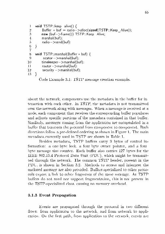
65

1 void TSTP::keep_alive() {2 Bu�er ∗ buf = radio−>alloc(sizeof(TSTP::Keep_Alive));3 new (buf−>frame()) TSTP::Keep_Alive;4 marshal(buf );5 radio−>send(buf);6 }78 void TSTP::marshal(Bu�er ∗ buf) {9 locator−>marshal(buf);10 timekeeper−>marshal(buf);11 router−>marshal(buf);12 security−>marshal(buf);13 }

Code Example 3.1: TSTP message creation example.

about the network, components use the metadata in the bu�er for in-teraction with each other. In TSTP, the metadata is not transmittedover the network along with messages. When a message is received at anode, each component that receives the corresponding bu�er populatesand adjusts speci�c portions of the metadata contained in that bu�er.Similarly, messages coming from the application are encapsulated in abu�er that traverses the protocol from component to component. Bothdirections follow a pre-de�ned ordering as shown in Figure 1. The mainmetadata currently used in TSTP are shown in Table 1.

Besides metadata, TSTP bu�ers carry 9 bytes of control in-formation: a one-byte lock, a four-byte owner pointer, and a four-byte message size counter. Each bu�er also carries 127 bytes for theIEEE 802.15.4 Protocol Data Unit (PDU), which might be transmit-ted through the network. The common TSTP header, present in thePDU, is shown in Section 3.2. Methods to access and interpret theenclosed message are also provided. Bu�ers specialized to other proto-cols export a link to other fragments of the same message. As TSTPbu�ers do not need nor support fragmentation, this is not present inthe TSTP-specialized class, causing no memory overhead.

3.1.3 Event Propagation

Events are propagated through the protocol in two di�erent�ows: from application to the network, and from network to appli-cation. On the �rst path, from application to the network, events are

66

Name Set by Used by MeaningRSSI MAC Locator Signal reception strength

for distance estimationSFD MAC Timekeeper Time of reception for

clock synchronizationID MAC MAC Message ID to detect

retransmissionsO�set Router, MAC Contention o�set for

MAC channel accessDestined Locator Router, Whether this messageto me MAC, API is destined to this nodeDirection Router Any Whether this message

goes towards the sinkDistance Locator Any This node's distance

to the destinationSender Locator Router Last hop's distancedistance to the destinationTrusted Security API, Whether the message's

MAC authenticity was veri�edRelevant Any MAC Signal the MAC that it

must receive the messageTransmissions MAC MAC Incremented each time the

MAC transmits this bu�er

Table 1: Main bu�er metadata used by TSTP.

implicitly propagated as components are invited to visit a bu�er in aprede�ned order through the invocation of speci�c methods that col-laboratively marshal a valid network packet. On the counter�ow, fromthe network up to the application, events are propagated using the Ob-server design pattern (GAMMA et al., 1995). When the network adapter�nishes copying a packet into a previously allocated bu�er and trig-gers an interrupt, that interrupt is handled by the Radio mediator andconverted into a noti�cation of an observed object (the Radio). TSTPprotocol components are therefore observers of zero-copy bu�ers, asillustrated in Figure 13.

Figures 15 and 16 show the sequence diagrams for sending andreceiving messages. Speculative space-time synchronization happensduring the execution of the Timekeeper's and Locator's update meth-ods. The send method of the API ends by inserting the message in the

67

transmission schedule, which is later consulted by the MAC. As the di-agrams denote, pointers to bu�ers are requested to the radio with theallocmethod, and only these pointers are passed through components,eliminating any copies of memory chunks.

Some network interface controllers feature a relatively large poolof hardware-accessible memory which is mapped into memory directlyaccessible by software. In these cases, the network hardware mediatormight return chunks of this memory as a result of calls to alloc, suchthat messages are constructed in-place, never leaving memory areasthat the hardware uses to send messages through the network. Someother devices, such as EPOSMote III, export a very limited amountof such memory, so that the radio mediator returns chunks of memoryfrom a pre-determined region of system memory, and copies it to radio-accessible memory only when the message is actually transmitted. Itis the responsibility of the radio mediator to manage this hardware-accessible memory. Whenever the radio mediator runs out of bu�ermemory, alloc returns 0.

3.1.4 Active Components

The main TSTP components are passive, i.e., do not execute ina dedicated thread and are triggered either by hardware interrupts orother active components, such as the application.

The MAC does not run in a dedicated thread, but implementsa state machine triggered by a dedicated hardware timer (Section 3.5).Figure 15 does not end with an actual message transmission, but ratheran enqueue operation on the MAC's transmission schedule. This sched-ule is consulted by the MAC's state machine when appropriate to actu-ally transmit the message. The MAC does not execute in a dedicatedthread because it needs to observe very precise timing (Section 3.5),and scheduling overhead could potentially compromise its correct func-tioning.

Figure 16 shows that the interrupt handler for received radiomessages reaches all the TSTP components, with a decoupling onlywhen the Application needs to be noti�ed. This design decision is alsomotivated by performance concerns, and components' update meth-ods can't perform time-consuming computations. When such compu-tations are needed, they should be decoupled from the critical pathof message processing. For example, for the more expensive key es-tablishment cryptographic operations, during system initialization the

68

alloc()

alloc()

get_b

uffer()

marsh

al(*b

uffer)

*buffer

*buffer

create_m

essa

ge(*b

uffer)

marsh

all(*b

uffer)

marsh

al(*b

uffer)

marsh

al(*b

uffer)

marsh

al(*b

uffer)

marsh

al(*b

uffer)

send(*b

uffer)

send(*b

uffer)

enqueue(*b

uffer)

Applica

tion

API

Radio

MAC

Locator

Timekeeper

Router

Security

Figure

15:Sequence

diagramfor

message

allocationand

transmission.

69

data

rece

pti

on in

terr

upt

pre

_noti

fy(*

buff

er)

acc

ept

noti

fy(*

buff

er)

update

(*buff

er)

synch

roniz

e(*

buff

er)

allo

c()

*buff

er2

copy(*

buff

er,

*buff

er2

)

send(*

buff

er2

)

update

(*buff

er)

synch

roniz

e(*

buff

er)

update

(*buff

er)

veri

fy_d

ecr

ypt(

*buff

er)

alt

update

(*buff

er)

update

(*buff

er)

copy_m

ess

age(*

buff

er)

noti

fy(c

opie

d_m

ess

age)

alt

notified

post

_noti

fy(*

buff

er)

free(*

buff

er)

free(*

buff

er)

alt

Radio

[acc

ept]

[!acc

ept]

MA

CO

bse

rved

Loca

tor

Tim

eke

eper

Route

r

[retr

an

smit

]

Secu

rity

API

[buff

er-

>tr

ust

ed]

Applic

ati

on

Figure16:Sequence

diagram

formessage

receptionandprocessing.

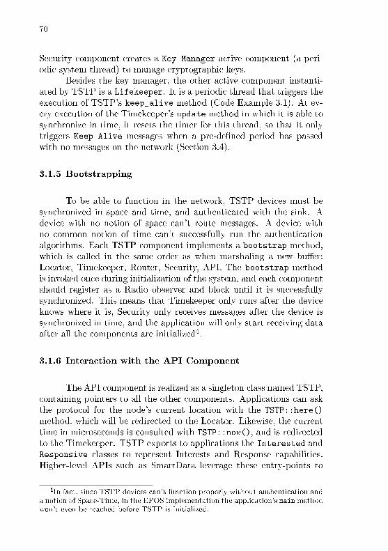
70

Security component creates a Key Manager active component (a peri-odic system thread) to manage cryptographic keys.

Besides the key manager, the other active component instanti-ated by TSTP is a Lifekeeper. It is a periodic thread that triggers theexecution of TSTP's keep_alive method (Code Example 3.1). At ev-ery execution of the Timekeeper's update method in which it is able tosynchronize in time, it resets the timer for this thread, so that it onlytriggers Keep Alive messages when a pre-de�ned period has passedwith no messages on the network (Section 3.4).

3.1.5 Bootstrapping

To be able to function in the network, TSTP devices must besynchronized in space and time, and authenticated with the sink. Adevice with no notion of space can't route messages. A device withno common notion of time can't successfully run the authenticationalgorithms. Each TSTP component implements a bootstrap method,which is called in the same order as when marshaling a new bu�er:Locator, Timekeeper, Router, Security, API. The bootstrap methodis invoked once during initialization of the system, and each componentshould register as a Radio observer and block until it is successfullysynchronized. This means that Timekeeper only runs after the deviceknows where it is, Security only receives messages after the device issynchronized in time, and the application will only start receiving dataafter all the components are initialized4.

3.1.6 Interaction with the API Component

The API component is realized as a singleton class named TSTP,containing pointers to all the other components. Applications can askthe protocol for the node's current location with the TSTP::here()

method, which will be redirected to the Locator. Likewise, the currenttime in microseconds is consulted with TSTP::now(), and is redirectedto the Timekeeper. TSTP exports to applications the Interested andResponsive classes to represent Interests and Response capabilities.Higher-level APIs such as SmartData leverage these entry-points to

4In fact, since TSTP devices can't function properly without authentication anda notion of Space-Time, in the EPOS implementation the application's mainmethodwon't even be reached before TSTP is initialized.

71

Header FormatBits: 3 2 1 2 8 3sb + 64 3sb + 64 0 or 32

24 - 46bytes

Time Location Origin Last Hop LocationVersion Type

RequestScale

Con�dence (x,y,z,t) (x,y,z,t) Deviation

Figure 17: TSTP common message Header format.

create powerful and elegant abstractions.

3.2 COMMON MESSAGE FORMATS

The TSTP message header is common to all TSTP messages,and every protocol component can access, parse, and modify any por-tion of the message. The TSTP header is shown in Figure 17. To enablerouting and passive synchronization, the header contains informationabout the node that is currently transmitting that message: its coor-dinates and the precise transmission time (Last Hop �elds), and itscon�dence in its own estimations of location (Location Confidence)and time (Time Request).

Besides characterizing the last node to transmit a message, theTSTP header characterizes the message itself. The Origin �elds indi-cate the time and place where the message was generated. The Version�eld identi�es the TSTP version of the message, which is currentlyalways set to 4. This �eld is packed �rst and matches the FrameType �eld in the Frame Control of IEEE 802.15.4 MAC packets. Aversion number above 3 renders TSTP into the reserved frame typezone (IEEE. . . , 2011), so that TSTP packets will not be erroneouslyinterpreted by other coexistent IEEE 802.15.4 nodes running di�erentprotocols.

Table 2 shows the meaning of values for the Scale �eld. Thesebits de�ne the size of each spatial coordinate (denoted sb) in the corre-sponding message, as well as a multiplier to be applied. For instance,with a Scale code 10, each x, y, and z coordinate shall have 16 bitsand represent multiples of 25cm, so a value of x = 3 would represent75cm. Such scaling makes these �elds adaptable to di�erent applica-tion scenarios, which may vary from, for instance, monitoring a smallroom to a large forest.

The possible values for the message Type �eld are shown in Ta-ble 3. A sink node announces interest in a physical quantity usingInterest messages. When receiving an Interest message, a sensornode checks if it is inside the desired region and able to measure the

72

Code Unit Scale Size (bits) Maximum Value

00 cm 50 8 127.5 m01 cm 1 16 655.3 m10 cm 25 16 16382.5 m11 cm 1 32 42949.6 km

Table 2: Spatial scaling codes.

Interest MessageBits: 192 - 368 4sb + 128 32 2 6 32 32

57 - 104bytes

RegionHeader

x,y,z,r,t0,t1Unit Mode Precision Expiry Period

Figure 18: TSTP Interest message format.

requested quantity with the required precision. If so, the Interest issaved and the node will automatically respond with a Response mes-sage every Period of time until the Interest expires, gets revoked, orthe node leaves the interested area.

Code Type

00 Interest01 Response10 Command11 Control

Table 3: TSTP message types.

The Interest message (Figure 18) speci�es the space-time Re-gion in which the Interest is valid (a sphere in space and a time inter-val), the desired SI Unit encoded according to the SmartData speci�ca-tion (Section 2.7), the periodicity of responses (Period), and minimumrequired Precision. Each measurement that is to be triggered by thisInterest will have an Expiry time associated to it, after which the sinkwill consider the data invalid. This Expiry is part of the SmartDataAPI5, and is used in TSTP only to detect and drop expired messageswhile they go through the network. The values of the Mode �eld areshown in Table 4.

Response messages (Figure 19) carry the SI Unit, detected mea-surement Error, the data Expiry as informed by the corresponding In-

5In SmartData, applications de�ne expiration times for each piece of SmartData.This value is used to inform scheduling decisions.

73

Code Type Meaning

00 Single Only one response is desired at each period.01 All Responses from all sensor nodes are desired

at each period.10 Revoke Revoke any interests with matching parameters.11 Unused

Table 4: TSTP Interest modes.

Response MessageBits: 192 - 368 32 8 32 Variable 128

65 - 119bytesHeader Unit Error Expiry Data MAC

Figure 19: TSTP Response message format.

terest, the Data itself, and a Message Authentication Code (MAC). TheSI unit and measurement Error are informed by characteristics of thephysical sensor that measured the data point. These characteristicsare also used to match local sensors to received Interest messages'Precision and Unit �elds. When necessary, the Security componentpads the data to a size suitable for its cryptographic engine (multiplesof 16 bytes for AES), encrypts the data, and signs it with a MAC.

Command messages (Figure 20) are treated similarly to Interest

messages, and are issued by the sink to trigger action from actuatornodes. This message type contains the desired Region of actuation,the SI Unit of the quantity to be acted upon, and a Value to applyto it. When directed towards speci�c sensor nodes, commands areencrypted and signed just as Response messages.

Control messages are used for various functions such as cryp-tographic key establishment or reporting of node capabilities, and allcarry the common control sub-header shown in Figure 21. The possibleSubtypes are shown in Table 5. The Control sub-header has plenty ofroom for introduction of new messages as TSTP evolves and incorpo-rates new features. The �rst four control message types concern secu-rity key establishment, and their corresponding messages are shown in

Command MessageBits: 192 - 368 4sb + 128 32 Variable 128

80 - 114bytes

RegionHeader

x,y,z,r,t0,t1Unit Value MAC

Figure 20: TSTP Command message format.

74

Control Sub-HeaderBits: 192 - 368 8

25 - 47bytesHeader Subtype

Figure 21: TSTP Control sub-header format.

Report MessageBits: 200 - 376 32 8 1 7

31 - 53bytes

Control EpochSub-header

Unit ErrorRequest

Unused

Figure 22: TSTP Report message format.

Section 3.6.

Value Subtype Value Subtype

0 ECDH Request 4 Report1 ECDH Response 5 Keep Alive2 Auth Request 6 Epoch3 Auth Granted 7 - 255 Unused

Table 5: TSTP Control subtypes.

Keep Alive control messages are �arti�cial� messages, contain-ing only the Control Sub-header (Figure 21) with Subtype 5. Nodesmay issue Keep Alives when they need to gather data for synchroniza-tion, but no message went through its neighborhood for some period oftime.

Report control messages are sent to the sink by sensor nodesafter they synchronize and authenticate. The node will send one suchmessage (exposed in Figure 22) for each transducer it has available,informing the Unit and Error associated with that device.

Inside the TSTP network, Space-Time is de�ned in relation toa pre-set reference (usually the sink's coordinates and clock), and thesink can convert the internal coordinate system to absolute Space-Time(coordinates relative to the Earth's center, and Unix time in microsec-onds) when data are to leave the network. In some cases, sensor nodesneed to know the parameters to convert from/to the internal coordi-nate system (e.g. a node with a GPS receiver needs to convert theGPS global coordinates to sink-centered coordinates; a sensor nodewith a display showing the date needs to convert local time to Unixtime). Sensor nodes with that need will set the Epoch Request bit ona Report Message, which will trigger a response from the sink in the

75

Epoch MessageBits: 200 - 376 3sb 64 96

48 - 79bytes

Control DestinationSub-header x,y,z

t0 x0,y0,z0

Figure 23: TSTP Epoch message format.

form of an Epoch control message (Figure 23), containing the absoluteSpace-Time coordinates of the center of the network.

3.3 POSITION ESTIMATION

The Locator component will include the node's current posi-tion and location con�dence in every message it sends. Non-anchornodes (with con�dence Cn < 100) maintain a list of the 3 non-collinearlandmarks with the best observed con�dence. A landmark is com-posed of a coordinate with an associated distance estimation and con-�dence greater than 80 (using estimated coordinates with low con�-dence leads to a very quick error propagation (REGHELIN; FRÖHLICH,2006)). Whenever a message is observed in the network, the receivingnode checks if the message's con�dence value is greater than its least-con�dent landmark, and if so replaces it, re-calculating its own positionand con�dence.

A lightweight geometry library was implemented for EPOS, whichis used by TSTP to store and parse coordinates, and also to perform 3Dtrilateration. The 3D Point parameterized class, depicted in Figure 24,takes the coordinate type as parameter, and its only data members arethe three coordinates. A Sphere contains a point and a radius. Bothclasses are compiled with the packed GCC attribute to make sure thatthe compiler will not add memory padding between data members.This way, coordinates or regions present in TSTP messages (e.g. Fig-ures 17, 18) are directly interpreted in-place as Point or Sphere, withno memory overhead. The Coordinate template parameter is a datatype of size according to the Scale used by TSTP, as shown in Table 2.

Variations of HECOPS have been implemented and evaluated us-ing di�erent techniques for two-dimensional spaces (REGHELIN; FRÖH-LICH, 2006; PIRES; WANNER; FRÖHLICH, 2008; GRACIOLI et al., 2011),which is generally not a suitable approximation for many TSTP sce-narios of interest (e.g. multi-�oor buildings). In the context of thepresent work, 3D localization functions were implemented. The Pointclass provides functions for performing translations, euclidean distance

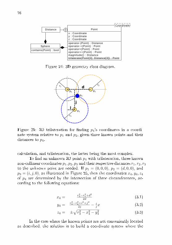
76

Distance

Sphere

contains(Point) : bool

Coordinate

Point

x : Coordinatey : Coordinatez : Coordinate

operator-(Point) : Distanceoperator-=(Point) : Pointoperator+(Point) : Pointoperator+=(Point) : Pointmagnitude() : Distancetrilaterate(Point[3], Distance[3]) : Point

Figure 24: 3D geometry class diagram.

r2r1

r3

p3

p2p1p4

d

j

i

Figure 25: 3D trilateration for �nding p4's coordinates in a coordi-nate system relative to p1 and p2, given three known points and theirdistances to p4.

calculation, and trilateration, the latter being the most complex.To �nd an unknown 3D point p4 with trilateration, three known

non-collinear coordinates p1, p2, p3 and their respective distances r1, r2, r3to the unknown point are needed. If p1 = (0, 0, 0), p2 = (d, 0, 0), andp3 = (i, j, 0), as illustrated in Figure 25, then the coordinates x4, y4, z4of p4 are determined by the intersection of three circumferences, ac-cording to the following equations:

x4 =r23−r

21+d2

2d (3.1)

y4 =r23−r

22+i2+j2

2j − ijx (3.2)

z4 = ±√r23 − x24 − y24 (3.3)

In the case where the known points are not conveniently locatedas described, the solution is to build a coordinate system where the

77

conditions are true. To achieve this, four operations must be appliedto the three known points: a translation of p1 to the origin, and threerotations to make y2 = 0 and z2 = z3 = 0. It is always possible to makeone of the coordinates zero for the three points, because three pointsde�ne a plane. The rotation angles are:

θx = arccos(y2)|p2| , θy = arccos(x2)

|p2| , θz = arccos(y3)|p3|

where |pn| is the magnitude of point n:

|pn| =√x2n + y2n + z2n (3.4)

Translation is done simply by subtracting all x coordinates byx1, y coordinates by y1, and z coordinates by z1. Using linear alge-bra techniques, the two rotations are arranged as a single 3x3 matrixthat performs all operations at once when multiplied to a point. Theresulting matrix is:cycz − sysxsz −szcx czsy + szsxcy

szcy + sysxcz czcx szsy − sxczcy−sycx sx cxcy

where cn = cos(θn), and sn = sin(θn).

After applying the translation and the rotation matrix, Equa-tions 3.1, 3.2, 3.3 can be applied to �nd the unknown coordinates inthe coordinate system based on p1, p2, p3. Afterwards, to return to theoriginal coordinate system, the inverse of the presented rotation matrixmust be applied to p4, and then the initial translation must be reversedby adding the original p1 coordinates to p4.

Translations, distances, magnitudes, and operations in the trans-formed coordinate system are reasonably simple, being adequate forWSN devices. The sine, cosine, and arc-cosine functions can be op-timized with lookup tables at the cost of accuracy. The matrix mul-tiplications are the most costly operations for WSN devices. Imple-mentation of a more e�cient algorithm for distance-based 3D localiza-tion (DOUKHNITCH; SALAMAH; OZEN, 2008) is left as future work.

3.4 TIME SYNCHRONIZATION

The Speculative Precision Time Protocol (SPTP) explores theprotocol's cross-layer architecture to speculatively peek through the

78

timestamps and geographic information present in TSTP headers withminimal insertion of explicit messages. A combination of low-leveltimestamping provided by TSTP's MAC, careful software implementa-tion leveraging the control granted by EPOS, and deterministic radiohardware provides the necessary basis for high-accuracy time synchro-nization.

3.4.1 Sources of Synchronization Imprecision

In the domain of energy-constrained IoT devices, no compensa-tion mechanism can achieve perfect target frequencies under practicalconditions. The IEEE 802.15.4 standard, for example, has a precisionrequirement for devices of ±40ppm, including temperature and agingvariations (MEHTA; PISTER, 2011). Because any two clock sources withdi�ering frequencies will always drift apart, a common measure of timebetween two independent systems requires a synchronization mecha-nism. The synchronization process itself is subject to temporal inac-curacies and variations. In the case of wireless IoT devices, these vari-ations arise from the message exchange process itself, which typicallyincludes the following steps:

1. Signal radio to enter transmission mode

2. Read the local timestamp

3. Copy message to the radio with the timestamp

4. Send Start of Frame Delimiter (SFD)

5. SFD is received

6. Receiver's current timestamp is recorded

The fundamental source of inaccuracy at the time of synchro-nization is the variation of the time interval (i.e. jitter) from acquiringthe sender's timestamp (step 2) to acquiring the receiver's timestamp(step 6). If this time was constant and quanti�able, even if very long,synchronization at the time of reading the timestamp would be perfect.This is however not the case in the majority of scenarios, since there aresources of jitter which may come from protocol design, software/hard-ware implementations, or physical phenomena. In NTP, for example,the delay is widely variable due to dynamic tra�c and congestion in themultiple hops between sender and receiver. In single hop scenarios with

79

a shared medium (such as wireless communications), the delay is vari-able due to medium access and propagation delays. Finally, even hostsusing switched networks with stricter timing guarantees may observejitter due to variations in software interrupt handling times.

In IEEE 802.15.4, the quality of timestamps (steps 2 and 6) isdictated by the standard, which imposes a minimum clock frequencyaccuracy requirement. The delay dTX involved in SFD transmission(steps 4 and 5) comes from software and hardware processing, mediumaccess, and signal propagation. Software processing can be measuredand made deterministic in many embedded systems. The jitter anddelay in medium access can be accounted for if the lower layers ofthe protocol stack are aware of the time synchronization mechanism:the MAC layer or the hardware itself can time-stamp messages aftermedium access, very close to the exact moment when it is to be sentthrough the physical medium. Apart from a deterministic time takento obtain timestamps right before/after an SFD is sent/received, theelapsed time between transmission and reception of timestamps is de-termined by delays provenient from signal propagation and processingat the physical layer. The former is negligible in the relatively shortdistances used in IEEE 802.15.4 links6; the latter is determined by theparticular hardware speci�cation, but mostly by the well-de�ned delayspresent in the standard:

sr = 62.5 symbolms IEEE 802.15.4 Symbol Rate

tu = 12sr

= 0.192ms IEEE 802.15.4 Turnaround TimeSPHR = 10symbol PHY header + preamble sizetPHR = 0.160ms PHY header + preamble time

and a more random component between SFD transmission and recep-tion caused by the process of synchronization between the sender's sig-nal modulator and the receiver's demodulator that takes place duringthe processing of the PHY preamble. Because this is the only compo-nent with inherent and non-negligible � but bounded � jitter, it deter-mines the limit for any software time synchronization strategy. Thisjitter is experimentally investigated in Section 4.2.3, and found to bein the order of nanoseconds for the target platform.

6Radio waves on air travel close to the speed of light.

80

3.4.2 SPTP Implementation

Clock synchronization is implemented as a collaboration betweenthe MAC and Timekeeper components. When a message is about to beinserted in the network, the MAC temporarily disables CPU interruptsand performs steps 1 to 4 listed above, including the raw reading ofthe device's timestamp counter in the Last Hop(t) �eld of the TSTPheader. Likewise, as soon as an SFD is detected, the MAC is responsibleto note the time of reception7 and attach it to the corresponding bu�er'smetadata. Timekeeper will take these timestamps to adjust the node'sclock according to Equations 2.3, 2.4.

Timekeeper is con�gured at compile-time with a characterizationof the timestamp transmission delay dTX , and the maximum tolerableperiod P between two clock adjustments, which is derived from theclock synchronization accuracy needed by the application (these pa-rameters are explored in Sections 4.2.3 and 4.4.3). Normally, clockadjustments run in speculative mode, just by the observation of net-work tra�c. Whenever the half-life of clock synchronization is reached(every P/2 units of time that pass without any message being observedin the network), Timekeeper will send a Keep Alivemessage to promptneighbors for timestamps. If P units of time pass with no messages,Timekeeper enters explicit mode, and will set the Time Request biton every message it transmits. Messages with this bit set are not usedby other nodes to synchronize, because it declares that the node send-ing it is not synchronized. In explicit mode, the node still sends KeepAlives every period P/2. The node goes back to speculative mode onceit successfully receives enough messages to adjust its clock.

3.5 MAC AND ROUTING

The MAC component interfaces the network with other TSTPcomponents while implementing a low duty cycle, receiver-based, packe-tized-preamble-sampling scheme that supports arbitrary metrics for re-lay selection. Figure 26 shows the activity diagram of TSTP MAC.The Update Transmission Schedule activity maintains the transmis-sion queue Qi (Section 2.5), checking for a pending bu�er transmis-sion. During Contend Channel Check, the node sleeps for a time de-�ned by the contention o�set Equation 2.7 and checks the channel.

7Some WSN devices such as EPOSMote III provide hardware support for notingSFD timestamps, and the MAC leverages it when available.

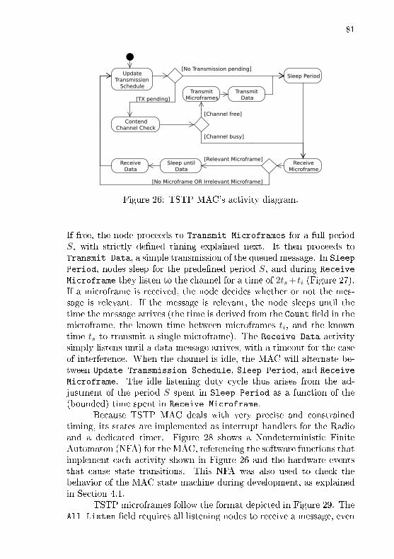
81

UpdateTransmission

Schedule

[TX pending]

ContendChannel Check

Sleep Period

ReceiveMicroframe

Sleep until Data

ReceiveData

TransmitMicroframes

TransmitData

[Relevant Microframe]

[Channel busy]

[Channel free]

[No Transmission pending]

[No Microframe OR Irrelevant Microframe]

Figure 26: TSTP MAC's activity diagram.

If free, the node proceeds to Transmit Microframes for a full periodS, with strictly de�ned timing explained next. It then proceeds toTransmit Data, a simple transmission of the queued message. In SleepPeriod, nodes sleep for the prede�ned period S, and during Receive

Microframe they listen to the channel for a time of 2ts+ ti (Figure 27).If a microframe is received, the node decides whether or not the mes-sage is relevant. If the message is relevant, the node sleeps until thetime the message arrives (the time is derived from the Count �eld in themicroframe, the known time between microframes ti, and the knowntime ts to transmit a single microframe). The Receive Data activitysimply listens until a data message arrives, with a timeout for the caseof interference. When the channel is idle, the MAC will alternate be-tween Update Transmission Schedule, Sleep Period, and Receive

Microframe. The idle listening duty cycle thus arises from the ad-justment of the period S spent in Sleep Period as a function of the(bounded) time spent in Receive Microframe.

Because TSTP MAC deals with very precise and constrainedtiming, its states are implemented as interrupt handlers for the Radioand a dedicated timer. Figure 28 shows a Nondeterministic FiniteAutomaton (NFA) for the MAC, referencing the software functions thatimplement each activity shown in Figure 26 and the hardware eventsthat cause state transitions. This NFA was also used to check thebehavior of the MAC state machine during development, as explainedin Section 4.1.

TSTP microframes follow the format depicted in Figure 29. TheAll Listen �eld requires all listening nodes to receive a message, even

82

MF MF

ts ts

ti

RX MF

tr

Figure 27: Microframe timing. If tr ≥ 2ts + ti, it is guaranteed thatreceiving nodes will have enough listening time to detect and receiveat least one microframe.

UpdateTransmission

Schedule

SleepPeriod

ε

ReceiveMicroframe

Sleep untilData

ReceiveData

ContendChannelCheck

TransmitMicroframe

TransmitData

ε

ε

ε

t

t ε

t

t

r

t t

r

r

t

t

Figure 28: TSTP MAC implementation's automaton. t transitionsare triggered by timer interrupts, r denotes radio interrupts, and εrepresents a transition that happens without a hardware interrupt (e.g.a function call at the end of the previous state's function).

83

Microframe FormatBits: 1 15 8 32 16

9bytes

AllListen

Id Count Distance CRC

Figure 29: TSTP microframe format.

those that wouldn't be candidates to relay it because they are furtheraway from the destination. It is used for control messages and for mes-sages whose destination is not a sink and therefore do not follow thedefault routing algorithm. The Count �eld is initialized by the sendingnode in accordance with S and decremented for each subsequent mi-croframe until the transmission of the message (after the microframewith Count = 0). This enables relay candidates to sleep until the timewhen the message is sent as long as they have listened to at least one mi-croframe. The Id �eld is initialized at the origin (i.e. at the node thate�ectively produced the data) and accompany the message unmodi�edacross the network until its destination. The purpose of this �eld is toreduce replication along the route, but not much e�ort is dedicated tomaking it unique since the destination has all the information it needsto detect a duplicate in the message's header (i.e. Origin(x,y,z,t)).It is currently implemented as a hash of the origin coordinates andtime. The Distance �eld holds the calculated distance between thetransmitting node and the message's destination, and allows listeningnodes to discard a message by listening to a single microframe whenAll Listen = 0 and Distance is smaller than the listener's distanceto the sink. CRC is used to discard corrupted microframes.

TSTP MAC takes a toll on senders and on overall latency toachieve low power consumption at receivers. The time ti between twoconsecutive microframes is set to a lower bound de�ned by the underly-ing communication technology (the IEEE 802.15.4 �turnaround time�),and the time ts to send a single microframe is �xed and known. Tocompensate for clock drifts, TSTP MAC de�nes that the idle listen-ing duration tr which happens every period S is 2ts + ti (Figure 27).Therefore, by setting the desired idle listening duty cycle d, the periodS can be determined as follows:

S = ts + (NMF − 1)× (ts + ti) (3.5)

where NMF is the number of microframes to be sent before each mes-

84

MF

ts

2ti + ts

MF

ts

ti ti Data

RX Data

RX DataS

≤ tr

RX MF

S

MF

ts

ti

ti

Sender

Receiver 1

S

≤ tr

RX MF

Receiver 2

Figure 30: TSTP MAC transmission example with NMF = 3. Receiver2 might wake up late due to clock drift and miss the �rst Microframe,but it receives the second one if tr ≥ 2ts + ti.

sage:

NMF = 1 +2ts+ti

d + ti + ts − 1

ti + ts(3.6)

Figure 30 shows a transmission example with NMF = 3. Thefollowing list shows the values of these parameters for an IEEE 802.15.4device.

sr = 62.5 symbolms IEEE 802.15.4 Symbol Rate

Tu = 12sr

= 0.192ms IEEE 802.15.4 Turnaround Timeti ≥ Tu Time between MicroframesSMF = 30symbol Microframe with PHY header sizets =

SMF

sr= 0.48ms Time to transmit a Microframe

tr ≥ 1.152ms Microframe listening time

3.5.1 Collisions and Hidden Nodes

Before transmitting any message, a node must sleep for a timeo�set according to a routing metric (Section 2.5.1) bounded by theMAC period S, then check the channel, and only carry on with trans-mission in case the channel is detected free. This contention mech-anism is appropriate to select relay nodes among contenders and toavoid collisions between neighboring nodes. However, it fails to solvemore complex cases of collisions involving non-neighboring nodes. Theproblem is demonstrated analyzing the tra�c captured from a set of

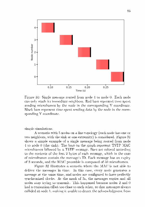
85

0.10 0.15 0.20 0.25Time (s)

0

1

2

3

4No

de n

umbe

r

Figure 31: Single message routed from node 4 to node 0. Each nodecan only reach its immediate neighbors. Red bars represent time spentsending microframes by the node in the corresponding Y coordinate.Black bars represent time spent sending data by the node in the corre-sponding Y coordinate.

simple simulations.A scenario with 5 nodes on a line topology (each node has one or

two neighbors, with the sink at one extremity) is considered. Figure 31shows a simple example of a single message being routed from node4 to node 0 (the sink). The bars on the graph represent TSTP MACmicroframes followed by a TSTP message. Bars are colored accordingto the contents of the �rst 2 bytes of each message, which in the caseof microframes contain the message's ID. Each message has an expiryof 3 seconds, and the MAC preamble is composed of 50 microframes.

Figure 32 illustrates a scenario where the MAC is not able todeliver the messages in time. In this case, every node generates amessage at the same time, and nodes are con�gured to have perfectlysynchronized clocks. At the mark of 3s, the messages expire and allnodes stop trying to transmit. This happened because nodes 2 and 0had a contention o�set too close to each other, so that messages alwayscollided at node 1, making it unable to detect the acknowledgment from

86

0.0 0.5 1.0 1.5 2.0 2.5 3.0 3.5Time (s)

0

1

2

3

4

Node

num

ber

Figure 32: Network tra�c with permanent collisions. Di�erent colorsrepresent messages with a di�erent ID. Shorter red bars represent colli-sions. All sensor nodes generate messages at t=0, but their contentiono�sets may di�er. At t≥0.5, nodes 1 and 2 are hidden nodes. Node1 transmits the purple message, which is received by the sink (node0). Then, the sink ACKs it, but node 2 is transmitting at the sametime, causing a collision at node 1. Then, node 1 retransmits it for notreceiving an ACK, and so on. This continues until the message expires,as contention o�sets are not changed.

node 0. Similarly, node 2 is under interference from node 3 and cannotdetect that node 1 is forwarding its message.

To solve this kind of permanent collision, a random backo� isintroduced at the MAC: every time it tries to transmit a bu�er, it in-crements a counter (stored as bu�er metadata) and adds to the bu�er'so�set a random value with upper bound proportional to that counter.In case the message is an ACK, it instead subtracts from the o�set.Figure 33 shows the same example with the random backo� employed.There are still collisions, but the backo� slowly pushes node 2 back andlets node 0 acknowledge node 1.

This kind of collision is a classic problem in WSNs, and is knownas the hidden node problem. It happens when two nodes detect a clear

87

0.0 0.5 1.0 1.5 2.0 2.5 3.0 3.5Time (s)

0

1

2

3

4

Node

num

ber

Figure 33: Network tra�c with random backo�. After each transmis-sion, a random component is added to the contention o�set of non-ACKtransmissions, so that hidden node situations eventually end.

88

0.0 0.5 1.0 1.5 2.0 2.5 3.0 3.5Time (s)

0

1

2

3

4

Node

num

ber

Figure 34: Collisions with sink at the middle with backo�. Nodes 1and 3 are often occupying the channel at the same time, so that Node2 (the sink) has a very small chance of correctly receiving a message.

channel for being out of range from each other and start a transmission.However, those messages will collide at a third node within communi-cation range of both transmitters. The random backo� can make thenodes desynchronize their transmissions over time to avoid permanentretries and collisions, but does not completely solve the problem. InFigure 34, the same setup is considered, except that node 2 is the sink.In this case where the sink is a hidden node, random backo� was notenough to deliver the messages in time.

To solve this problem, every node that transmits a non-ACKmessage will be prevented from transmitting again for a number ofMAC periods. This gives receivers of the transmitted message a chanceto acknowledge it and forward it out of the hidden node area (POLAS-TRE; HILL; CULLER, 2004). To implement this, the MAC will keep acounter of how many times any given bu�er was (re-)transmitted in thepast. Every time it transmits a bu�er that is not an explicit acknowl-edgment, it increments the counter and will not transmit any messagefor a random number of periods between 1 and the counter value. Fig-ures 35, 36 show that random periods of silence combined with random

89

0.0 0.5 1.0 1.5 2.0 2.5 3.0 3.5Time (s)

0

1

2

3

4No

de n

umbe

r

Figure 35: Collisions with sink at the end with backo� and silence.After a transmission, a node will not transmit anything for a random-ized number of MAC periods. This gives nodes more time to ACK themessages, and hidden node situations are solved quicker.

backo�s successfully solve the collisions in the observed cases, decreas-ing total radio activity time and greatly improving end-to-end delay.

To further reduce the cases of interference, a multichannel tech-nique is also introduced. All microframes are sent in a pre-determined,�xed channel, but their corresponding data messages are sent in achannel determined by the message's ID (which is included in themicroframe). This way, a node may wake up, receive a microframecorrectly, sleep and wake up to receive the data message (in anotherchannel) successfully, even if another node started transmitting its ownmicroframes in the meantime, while that node was sleeping (the othernode's microframes would collide with the data message if they were inthe same channel).

90

0.0 0.5 1.0 1.5 2.0 2.5 3.0 3.5Time (s)

0

1

2

3

4

Node

num

ber

Figure 36: Collisions with sink at the middle with backo� and silence.At around t=0.7, the periods of silence from nodes 1 and 3 are longenough that node 2 has the chance to correctly receive and acknowledgethe messages.

91

3.6 SECURITY

As explained in Section 2.6, TSTP's security mechanisms arebased on Elliptic-Curve Di�e Hellman (ECDH) for initial establish-ment of symmetric keys exchanging two messages: ECDH Request andECDH Response. Afterwards, Poly1305-AES is used to combine uniquesensor IDs and synchronized time-stamps for generation of One-Time-Passwords (OTP) used to authenticate those keys by exchanging twomore messages: Auth Request and Auth Granted. Cryptographic keysare never used directly, but combined as OTPs which are then used asAES symmetric keys to sign, verify, encrypt, and decrypt messages.

AES is an attractive cryptographic engine because of the rela-tively common presence of hardware accelerators for it in WSN devices,in part due to it being adopted by the IEEE 802.15.4 standard. AEShardware accelerators are used by the Security component when avail-able (such as in EPOSMote III), and a software implementation isprovided otherwise (such as in OMNeT++). AES realizes the Cipherinterface, which simply exports an encrypt and a decrypt methodthat are used by TSTP. The actual AES implementation to be usedis de�ned at compile-time with static metaprogramming techniques,incurring no runtime overhead.

To support the ECDH operations, a Bignum library was devel-oped for EPOS (RESNER, 2014) to implement prime �nite �eld arith-metics with large numbers. It uses the thin template technique toprovide an elegant and light interface to interact with arbitrary-sizedarrays of �digits�, each digit being a native word of the CPU. TheBignum library uses the Barrett Reduction algorithm to implement ef-�cient addition, subtraction, multiplication, and inversion modulo alarge prime number. An ECDH library was developed on top of thisBignum implementation, with e�cient elliptic-curve point multiplica-tion using jacobian and a�ne coordinates. TSTP currently works witha key size of 128 bits.

The Poly1305 implementation uses the Bignum library for itsoperations modulo 2130 − 5, and the Cipher for its interaction withAES, being as e�cient as those implementations.

3.6.1 Key establishment and management

Although TSTP's security mechanism is currently used to es-tablish end-to-end encryption and authentication between the sink and

92

Peer-id: Node_ID-auth: Node_ID-ms: Master_Secret-auth_time: Time-valid: Region

Peer

List*

Figure 37: Security component's Peer data structure.

Pending_Key

List

Pending_Key-creation: Time-pk: Public_Key-ms: Master_Secretmaster_secret(): Master_Secret

*

Figure 38: Security component's Pending_Key data structure.

each sensor node independently, its design does not prevent sensornodes from acting as masters, or from establishing keys with multiplemasters. The Security component's data structures are implementedin a way to re�ect that, naturally supporting expansion to group keys,sensor-to-sensor keys, or multiple sinks, as well as providing a uniformkey management interface for masters and slaves.

The Security component maintains two lists of Peers, which arecalled pending_peers and trusted_peers, and a list of pending_keys.Figures 37, 38 show simpli�ed diagrams of these data structures.

At any time, a master can add Peers to the pending_peers list,representing a slave node that will eventually try to authenticate withthis master. It initializes the data structure with the ID and Auth ofthe slave, and a space-time region in which that node is allowed toauthenticate. Upon insertion of the �rst slave, a master will start a keymanagement thread, which will periodically examine both lists of peersto remove expired entries and send ECDH Request messages (Figure 39)to valid pending peers8.

ECDH Request MessageBits: 200 - 376 3sb 384

76 - 107bytes

Control Destination PublicSub-header x,y,z Key

Figure 39: TSTP ECDH Request message format.

At bootstrap time, a slave will instantiate a Peer containing its

8The study of appropriate key manager periods and key expiration times are notin the scope of this work.

93

own ID and Auth, and a space-time region centered at the coordinatesof the master, radius 0, and time equal to the expected lifetime of thenode.

Upon reception of an ECDH public key (either a slave receivingan ECDH Request message or a master receiving an ECDH Response �Figure 40), a node will check if there are any pending peers, and ifso, save the public key and the current time in a Pending_Key objectand insert it in the pending_keys list. The public key is only usedto calculate the Master Secret, but the Pending_Key object saves it touse lazy evaluation, calculating the Master Secret only the �rst time itis actually accessed (by means of the master_secret method). Thisprevents the costly ECDH point multiplication in cases where the up-coming authentication step fails.

ECDH Response MessageBits: 200 - 376 384

73 - 95bytes

Control PublicSub-header Key

Figure 40: TSTP ECDH Response message format.

Upon reception of an OTP (either a master receiving an Auth

Request � Figure 41 � or a slave receiving an Auth Granted message �Figure 42), the node tries each possible pending key/pending peer pairto generate a matching OTP. Once it does, the Master Secret is copiedto the Peer, its authentication time is registered, that Peer moves tothe trusted_peers list, and the Pending_Key is removed from thepending_keys list and destroyed.

Auth Request MessageBits: 200 - 376 128 128

57 - 79bytes

ControlSub-header

Auth OTP

Figure 41: TSTP Auth Request message format.

Auth Granted MessageBits: 200 - 376 3sb 128

44 - 75bytes

Control Destination AuthSub-header x,y,z OK

Figure 42: TSTP Auth Granted message format.

The trusted_peers list is checked by the Security component to�nd the necessary shared secrets to encrypt, decrypt, sign, and verifyeach message.

94

3.7 SMARTDATA

The SmartData API is out of scope for the present work. Smart-Data is seen as �application� by TSTP, and none of the evaluations inthis work consider it. From TSTP's perspective, applications can in-teract with it using a full implementation of SmartData � such as inthe EPOS implementation, � or a minimalist compatibility layer � suchas in the OMNeT++ implementation.

95

4 TSTP EVALUATION




The wide range and complexity of TSTP requires a performanceevaluation using di�erent approaches and tools. This chapter tack-les validation and performance evaluation from di�erent angles: animplementation for the EPOSMote III platform allows validation ofthe protocol in real-world deployments, as well as measurements thatare heavily in�uenced by environment or hardware conditions (such astime synchronization); a simulator implementation allows debuggingin a controlled environment, as well as analysis of arbitrary statisticsfrom a wider range of deployments and parameter combinations; ananalytic model of network behavior is developed and its predictionsare compared against simulation results; code overhead is analyzed forboth the simulator and real-world implementations; trace visualization,code pro�ling, and other tools are used to help debug and optimize im-plementations.

4.1 TOOLS AND DEBUGGING

The distributed nature of WSNs, combined with the hardwareconstraints of the devices involved, results in a development environ-ment that can be challenging to test and debug. A series of tools wereused and developed to help this process. This section brie�y presentsthese tools, as well as the steps taken to make simulations run faster.

4.1.1 MAC State Machine Veri�cation

To verify the state transitions of the MAC, the code was instru-mented during development to indicate, by printing speci�c characterson the screen, whenever a MAC timer or radio hardware interrupt

96

happens, and whenever a MAC state is entered (Section 3.5). Theseexecution traces are processed by a separate C++ program which im-plements an NFA with the same structure as the MAC's (Figure 28)and checks whether any state violation is found. This process is spe-cially important for the EPOS implementation because EPOS allowsInterrupt Service Routines (ISR) to be preempted. ISR preemption be-comes more likely to occur as the MAC deals with events that happenclose to each other in time. The check of execution traces producesevidence that there is no unintended preemption of handlers that leadsto inconsistent state transitions.

4.1.2 Security Library Veri�cation

For verifying the big integer library used in security (Section 3.6),an EPOS application was developed that generates random numbersand operations, operates them, and prints the numbers, operation, andresult with Python list syntax. Then a Python program (which natu-rally supports big integer arithmetics) parses the outputs, reproducesthe operation, and checks the results, reporting any errors at the end.A sample EPOS output is shown below.

Bignum Utility Testsizeof (Bignum<16>) = 16 bytes.sizeof (Bignum<16>::Digit) = 4 bytes.Random seed = 12345Modulo = [4294967294, 4294967295, 4294967295, 4294967293] +1a = [229283573, 3596950572, 2802067423, 3554416254]b = [2941955441, 3441282840, 1051550459, 3256818826]a + b = [3171239015, 2743266116, 3853617883, 2516267786]a = [3490719589, 1157490780, 3144468175, 3866696494]b = [2103497953, 1538207304, 1511588075, 2684337210]a ∗ b = [180798668, 400923757, 2054889077, 1345744013]

The Elliptic Curve Di�e-Hellman library is tested with an appli-cation that generates many random public-private key pairs, operatesthem, and checks whether the resulting shared keys match. Poly1305-AES signatures are tested against known vectors (BERNSTEIN, 2005), aswell as rounds of signing random messages and verifying the signature,then verifying with wrong parameters.

97

4.1.3 Network Tra�c Visualization

Network traces are useful to verify message formats, timings,and general network behavior. The packet capture (pcap) �le formatprovides a popular and simple syntax for storing network tra�c traces,which can be parsed by high-level visualization tools such as Wireshark.A simple C++ pcap formatting library was written for EPOS suchthat a sni�er node can capture tra�c without any interference on theobserved network. The library was also included in the OMNeT++code and can be used in the simulations to capture all the generatedtra�c.

A Wireshark plugin was written to enable it to parse TSTP traf-�c. The pcap header indicates that tra�c type is IEEE 802.15.4, sothat Wireshark loads the appropriate dissector. The IEEE 802.15.4dissector was modi�ed to identify any 9-byte packet as a TSTP mi-croframe (9 bytes is not an allowed IEEE 802.15.4 frame size), andany packet with size greater than 9 and a reserved Frame Type as aTSTP message. In these cases, it calls the TSTP dissector for furtherprocessing. Figure 43 shows a sample Wireshark session.

4.1.4 Simulation Execution

Thousands of simulation experiments were performed in the con-text of the present work, many of which took hours to complete, justify-ing e�orts towards code optimization and e�cient usage of computingresources. As simulations are numerous, independent, and CPU-bound,a suite of scripts was developed to execute them in parallel, each as aseparate Linux process. The scripts deploy the simulations to a 36-core Amazon AWS virtual machine, spawning 36 Linux processes andreporting 100% usage on all CPUs. Simulation runs are randomly as-signed to each CPU to avoid particularly long combinations of runs.

Parallelism is not explored within simulation runs, as it would bea more complex task with risks of introducing errors. Instead, to opti-mize individual runs, a sample simulation was pro�led using Valgrind'scallgrind tool, with kcachegrind for visualization. kcachegrind

showed that a signi�cant portion of time was spent in Castalia's tracegeneration methods, even when traces were disabled. A pre-compilermacro was added to allow a more aggressive compile-time removal ofthese methods when they are not desired, and run times were signi�-cantly reduced.

98

Figure 43: Analyzing a TSTP pcap trace with Wireshark.

99

4.2 EPOSMOTE III EXPERIMENTS

Two implementations of TSTP are analyzed in this chapter. At�rst, TSTP was implemented in C++ for the EPOS Operating Systemand the EPOSMote III platform, an IoT device based on Texas In-strument's CC2538 System-on-Chip with an IEEE 802.15.4 radio andARM Cortex-M3 processor at 32MHz.

TSTP's component-based implementation and a programminglanguage compatibility allowed it to be ported from EPOS to the OM-NeT++ simulator with the Castalia framework without many changes:mostly rewriting EPOS' network interface mediator to handle Castalia'sRadio framework, and the TSTP API component's noti�cation methodto interact with Castalia's application layer1. As a result, the simulatorframework implements a very detailed model of a real TSTP network,with simulated network devices running code very similar to what isrun on real EPOSMote III devices.

Castalia code was compiled on/for an Intel Core i5-2320 CPU,with g++ version 4.8.5-2ubuntu1 14.04.1 on an x86_64 Ubuntu 14.04Linux Operating System. EPOS code was cross-compiled on the samehost machine with g++ version 4.4.4 for the ARM Cortex-M3 proces-sor. By the time of this writing, all the source code is freely availableat https://epos.lisha.ufsc.br.

4.2.1 Code Size

Table 6 shows the resulting compiled code size for each protocolcomponent. It shows EPOS' and Castalia's implementations of eachTSTP component, compared with two third-party implementations ofthe AODV protocol, a simple implementation of IEEE 802.15.4 unslot-ted CSMA/CA MAC for Castalia and EPOS, and BypassRouting, avery simple network layer in Castalia that forwards messages directlybetween the MAC and application layers. The full TSTP implementa-tions comprising all of the components achieve a code size close to theAODV implementations, which only provide routing.

1A few other technical changes were necessary, such as the removal of staticmethods and class attributes, which in Castalia are shared across every node in thesimulated network.

https://epos.lisha.ufsc.br

100

Component Castalia code size EPOS code sizeTimekeeper 1721 3728Locator 2687 3048Router 3134 3606MAC 4873 7644API 9936 7434

Security 11148 8322Total 33499 33782

BypassRouting 1196 -802.15.4 MAC 5534 3546

AODV 1 29567 -AODV 2 34513 -

Table 6: Code size (bytes) for TSTP components and other protocols.

4.2.2 Bu�er Management

As explained in Section 3.1.1, TSTP uses a relatively simpleversion of EPOS' zero-copy bu�er and a system heap to allocate bu�erse�ciently. Apart from TSTP metadata and the IEEE 802.15.4 PDU,the bu�er uses a one-byte lock, a four-byte owner pointer, and a four-byte size counter as control information, summing up to 9 bytes ofoverhead.

The time overhead for allocation of bu�ers was measured on twoEPOSMote III devices running TSTP, one acting as a sink and the otheras a sensor node. The two nodes allocated a total of 260548 bu�ers,taking on average 2.31µs for each allocation. For the experiments inthis section, hardware interrupts were disabled during the execution ofthe code parts being assessed.

The mechanism for propagating received bu�ers throughout thecomponents explained in Section 3.1.3 was evaluated on the same EPOS-Mote III devices. The time a bu�er enters and leaves each componentwas recorded to �nd the propagation overhead in relation to the totalprocessing time. For 278800 measurements, the average time for eachbu�er to leave the MAC, be processed by the other components, andreturn to the MAC (as depicted in Figure 1) was 108.57µs. From thistime, on average 12.60µs were spent between the end of a component'supdate method and the start of the next, accounting for the overheadof the noti�cation mechanism itself, which represented 11.60% of thetotal bu�er processing time. Table 7 summarizes these measurements.

101

Bu�ers allocated 260548Avg. bu�er allocation time 2.31µsReceived bu�ers processed 278800Avg. bu�er processing time 108.57µs

Avg. notify time 12.60µsNotify time / processing time 11.60%

Table 7: Assessment of time overhead for bu�er management.

4.2.2.1 Integrity Control

Since every component has access to the full message data andmetadata, it is not easy to guarantee that components will not changepieces of information that other components may use in another way.There is no intra-node integrity control in the current implementation ofthe zero-copy bu�er. Besides added overhead, it is not straightforwardto enforce integrity, because one of the design goals for the currentimplementation is to keep the components free to use and modify anyinformation, as well as make it easier to try new, previously unexpectedsubcomponents. The only form of control currently implemented isthe well-de�ned order in which the components' methods for handlingbu�ers are called, as illustrated in Figure 1.

4.2.3 Time Synchronization

The following experiments investigate the limits of time syn-chronization obtainable in the physical platform. As explained in Sec-tion 3.4.1, the jitter in timestamp processing de�nes the limits of clocksynchronization for a given implementation, and arises from the elapsedtime in the following steps:

1. Signal radio to enter transmission mode

2. Read the local timestamp

3. Copy message to the radio with the timestamp

4. Send Start of Frame Delimiter (SFD)

5. SFD is received

6. Receiver's current timestamp is recorded

102

●

●

●

●

Node 1 Node 2

3.05

3.10

3.15

3.20

SF

D d

elay

(us

)

Figure 44: Jitter in Start of Frame Delimiter transmission.

SCHMID; DUTTA; SRIVASTAVA determined the SFD jitter (steps4 and 5) on the CC2420 platform by measuring the time between thehardware SFD signal (exported by the platform as GPIO) at the senderand at the receiver, and reported that 95% of measurements fell withinan interval of 160ns (SCHMID; DUTTA; SRIVASTAVA, 2010). For thepresent work, this experiment was replicated on the EPOSMote IIIplatform. In the setup, one node transmits messages periodically andtwo other nodes listen. The nodes were positioned close to each other(less than 30cm away) with no obstacles in between. The SFD signals(also exported by the platform as GPIO) are observed at each of thethree nodes with an oscilloscope and their time di�erences are noted.The delays observed range from 3.038µs to 3.225µs, representing aninterval of 187ns (Figure 44). Using the average value of 3.1315µs,the maximum unpredictable variation of the actual delay for a giventransmission is 93.5ns. This number represents the hardware-imposedlimit a synchronization protocol can consistently get at the instant ofclock o�set determination between two nodes.

Acquiring timestamps close to SFD transmission and receptiontimes requires precise control and predictability in the software stack.In general-purpose systems such as Linux, the wide variability in I/Oand interrupt handling timing makes it virtually impossible to accu-rately quantify the time between these two operations, and hence im-plementations of protocols such as PTP require hardware timestampingfor high-precision synchronization. With hardware timestamping, the

103

network interface itself acquires a timestamp as soon as SFD or equiv-alent frame delimiters are sent or received. In this work, by disablinginterrupts during the short period between message timestamping andtransmission and using only deterministic software instructions duringthis time, the processing delay is accurately compensated. The timefrom the start of step 1 (�Signal radio to enter transmission mode�) tothe end of step 4 (�Send Start of Frame Delimiter�) was measured withan oscilloscope over several runs of the implementation in question, andit is 352.17µs, 170ns above the IEEE 802.15.4 expected time for theradio to get ready and send the physical layer headers (tu + tPHR),with a detected jitter equal to the oscilloscope's own period (5ns). Theradio hardware itself records timestamps of received messages, and sothe delay between SFD reception and timestamp recording (steps 5and 6) is considered to be zero. Therefore, the combination of low-leveltimestamping provided by TSTP's MAC, careful software implementa-tion leveraging the control granted by EPOS, and deterministic radiohardware successfully provides the necessary basis for a high-accuracytime synchronization protocol.

To evaluate the performance of the time synchronization algo-rithm, four motes were set up in a star topology distributed in positionssimilar to the previous experiment. Three motes are receivers and oneis a transmitter, which sends timestamps at a constant interval of 3seconds (Figure 46), 15 seconds (Figure 47), or 30 minutes (Figure 48).Each receiver node listens to every message and independently syn-chronizes with the transmitter. When a message arrives at time ti,the receiver �rst gets cN (t′i) (Section 2.4) without any o�set correction,then calculates cN (ti) as an estimation with its previous calibrationvariables of what the value of cN (ti) is going to be after instant o�setdetermination. It then calculates its immediate o�set from the sender(Equation 2.3), updates its clock drift estimation (Equation 2.4), cal-culates cN (ti) taking into account the calibration just performed, andgets the error as cN (ti) − cN (ti). Figure 45 compares the instant o�-set at the moment of message reception with the previously estimatedcorrection values during execution of Node 1 in Figure 46. The erroris the di�erence between the two. In Figures 46, 47, 48, only the errorand instant o�set values are shown.

More than achieving a sub-microsecond instant synchronizationper-hop close to the physical limit that is comparable to high-precisionprotocols such as PTP, the results show that on a network with tra�c ofone message every three seconds, SPTP keeps the network synchronizedto sub-microsecond accuracy at all times without insertion of any extra

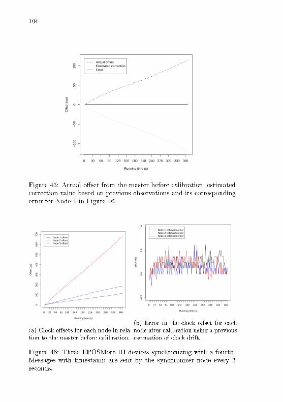
104

−10

0−

500

5010

0

Running time (s)

Offs

et (

us)

0 30 60 90 120 150 180 210 240 270 300 330 360

Actual offsetEstimated correctionError

Figure 45: Actual o�set from the master before calibration, estimatedcorrection value based on previous observations and its correspondingerror for Node 1 in Figure 46.

010

020

030

040

050

060

070

0

Running time (s)

Offs

et (

us)

0 27 54 81 108 144 180 216 252 288 324 360

Node 1 offsetNode 2 offsetNode 3 offset

(a) Clock o�sets for each node in rela-tion to the master before calibration.

−0.

50.

00.

51.

0

Running time (s)

Err

or (

us)

0 27 54 81 108 144 180 216 252 288 324 360

Node 1 estimation errorNode 2 estimation errorNode 3 estimation error

(b) Error in the clock o�set for eachnode after calibration using a previousestimation of clock drift.

Figure 46: Three EPOSMote III devices synchronizing with a fourth.Messages with timestamp are sent by the synchronizer node every 3seconds.

105

050

0010

000

1500

020

000

2500

0

Running time (s)

Offs

et (

us)

0 2250 4500 6750 9000 11250 13500



−5

05

1015

Running time (s)

Err

or (

us)

0 2250 4500 6750 9000 11250 13500



Figure 47: Three EPOSMote III devices synchronizing with a fourth.Messages with timestamp are sent by the synchronizer node every 15seconds.

050

010

0015

0020

00

Running time (min)

Offs

et (

ms)

0 300 600 900 1500 2100 2700 3300



−20

0−

100

010

020

030

0

Running time (minutes)

Err

or (

us)

0 300 600 900 1500 2100 2700 3300



Figure 48: Three EPOSMote III devices synchronizing with a fourth.Messages with timestamp are sent by the synchronizer node every 30minutes.

106

η Average number of non-sink neighbors each node hasH Average number of hops between each node and the sinkλ Data generation rate of the whole networkS MAC contention period

Table 8: Analytic model parameters.

message (while PTP, for instance, requires at least 3 explicit synchro-nization messages). This accuracy gets worse as tra�c becomes moresparse, reaching observed worst cases of almost 15µs with a messageperiod of 15 seconds, and around 300µs for 30 minutes.

4.3 ANALYTIC MODEL

The development of an analytic model to predict network be-havior under di�erent con�gurations serves several purposes: it helpsunderstand the way that di�erent factors contribute to di�erent met-rics of interest such as average latency or network lifetime; it aids thedeployment of new networks, or new sensors on a network, by quicklypredicting whether a network with given topology and average data ratewill be saturated or close to saturated; it also helps validate the sim-ulator and real-world implementations by comparing their predicted,simulated, or observed behaviors. When used as a network design tool,the analytic model is not meant to be as complex and accurate as thesimulator, but much easier and faster to use, providing preliminaryinsight to designers of new networks.

The whole network is modeled as an M/M/1 queue, which rep-resents a system with a single server, where events arrive accordingto a Poisson process and job service times have an exponential distri-bution. Events represent sensor readings that trigger application datamessages, and the job service time denotes the total latency betweendata creation at a sensor node, routing through the network, and ac-knowledgment by the sink. An M/M/1 queue takes as parameters thearrival rate λ and the mean service rate µ.

The proposed model takes 4 parameters, shown in Table 8. Thearrival rate is taken directly as a parameter, and the other three serveto de�ne the mean service rate µ as the average rate at which TSTP candeliver end-to-end messages, considering aspects of topology, collisions,and MAC con�guration.

Before sending a message, TSTP MAC determines that a node

107

must pick a time interval called o�set bounded by the contention periodS, wait for that time, start clear channel assessment, and proceed totransmit the message only if no channel activity is detected. The timeto send a one-hop message that does not cause collisions is given byEquation 4.1, assuming that the average o�set is half the contentionperiod, CCA takes TCCA time, data transmission takes Td time, andthe MAC preamble takes S time.

T1 = (1.5× S) + TCCA + Td (4.1)

A contention slot is de�ned as the minimum time di�erence nec-essary between two nodes starting CCA so that one of them will detectthe subsequent transmission by the other. In IEEE 802.15.4, it is 160µs.Given that contention periods are composed of Cs contention slots, thato�sets are chosen at random, and that there are n contending nodes,the probability of any two contenders colliding is determined as theprobability of at least two nodes starting CCA at the same contentionslot, which is the complement of the probability that every node willpick a di�erent slot, given by Equation 4.2.

Pc(n) = 1− Cs!

(Cs − n)!× Cns

(4.2)

Because of the MAC silence mechanism (Section 3.5.1), it is ap-proximated that the ith consecutive collision for a given message willcost (S+TCCA)× i of silencing time, and that the following contentionround will have half as many contending nodes. The estimated cost ofsending a one-hop message, given that N other nodes are contending,and that i consecutive collisions already happened for this message, isthus:

Ec(N, i) =Pc(N + 1)

× (T1 + (S + TCCA)i+ Ec(bN/2c, i+ 1))

+ (1− Pc(N + 1))× T1(4.3)

The mean service rate is de�ned in Equation 4.4 as the aver-age time a message takes to travel H hops, considering the costs ofcollisions.

µ =1

Ec(η, 0)×H(4.4)

Metrics of interest are then derived from closed-formula values

108

given by the M/M/1 queue model. Average latency is the queue'saverage service time. Delivery ratio is interpreted as the probability ofthe service time being higher than the average data generation period,which is given by the exponential distribution with parameter µ× (1−λ/µ). Energy consumption is derived from the probability Pa of theMAC being active, which is the queue's probability of having at leastone job being processed in the queue. For network lifetime estimations,it is considered that a given node will be active with probability Pa/2,and when active, 75% of the time it will be for receiving a message, andthe other 25% for transmitting. The model's predictions are shown inthe next section, along with simulation results.

4.3.1 Limitations

The presented model is a simplistic approximation of networkbehavior in many senses: it assumes that all nodes are homogeneous,with the same behavior and surrounding network tra�c, which is gen-erally not the case (e.g. nodes closer to the sink tend to handle moremessages); the model of collision overhead and resolution is fairly sim-ple; it completely ignores other relevant e�ects such as radio signal loss,dropping of expired messages, message duplication along the route, ex-plicit synchronization messages, etc.

The predictions made by the model are only valid when the net-work is not saturated, since the M/M/1 queue requires that the servicerate is higher than the arrival rate.

4.4 SIMULATION EXPERIMENTS

This section presents results from simulations with TSTP's im-plementation for the OMNeT++ simulator with the Castalia frame-work. For the remaining of this chapter, the following simulation sce-narios are considered: environment monitoring and o�ce. Theenvironment monitoring scenario models a WSN that monitors slowlychanging environmental conditions such as temperature or humidity. Ithas the following characteristics:

• sparse, constant tra�c, with a data period of 60s, 300s, 600s,900s;

• data expiries equal to period;

109

• regular placement (Figure 49) on a 500m x 500m �eld with sinknode at the center;

• clean channel: free space model, symmetric radio ranges of ≈100m;

• static nodes;

• initial battery charge for every node: two AA batteries (18720J).

The o�ce scenario models an o�ce building with:

• heterogeneous tra�c (data period):

� 10% of nodes at 300ms, expiry = 300ms;

� 20% of nodes at 1s, expiry = 1s;

� 60% of nodes at 10s, expiry = 1s;

� 10% of nodes at 1min, expiry = 300ms;

• two di�erent placements according to real-life o�ce maps: LISHA(14 nodes, Figure 58) and SSB (40 nodes, Figure 64)

• lossy channel;

• static nodes;

• initial battery charge:

� two AA batteries (18720J) for 1min nodes and 50% of 10snodes;

� in�nite battery for remaining nodes.

These characteristics are also presented in Tables 9, 11, 12, wheneach scenario is analyzed. In all of the scenarios, the sink node hasin�nite energy supply, and applications start producing periodic dataafter a random time o�set of at most one data period. Each simulationruns for 2 hours (simulated time).

4.4.1 Sources of Random Variation

Each simulation experiment is run with di�erent seeds for thepseudo-random number generators. This seed impacts aspects of thesimulation that in�uence the measured results, even between replicatedruns with otherwise identical input parameters. The main sources ofrandom variation in the measured output variables are:

110

• Each node generates a new data message with a �xed period d.Before sending the �rst message, each node n waits for a randomtime tn < d, and proceeds to send a message every d period.Depending on the distribution of these random o�sets, nodes maygenerate messages closer in time, which increases the momentaryworkload of the network and reduces overall performance;

• The random backo�s and silence periods in the MAC (Section 3.5.1)a�ect the overall number of message collisions;

• Physical channel e�ects on the radio signal;

• The clock frequency error for each node is initialized with a ran-dom component of at most 40ppm.

4.4.2 MAC Con�guration

Correctly con�guring MAC and radio parameters for TSTP isnot a trivial task. By increasing radio transmission power, nodes willspend more energy to transmit the same amount of data, but radiorange will increase and potentially less hops will be needed to reach the�nal destination, saving energy across the network. Likewise, increasingthe length of the MAC preamble causes senders to occupy the channelfor a longer time before each data transmission, but allows receivers tosleep for the same, longer, amount of time. There is an optimal con�g-uration for both radio transmission power and MAC preamble length,which is dependent on the network characteristics. The following setof experiments analyze the impact of MAC con�gurations to identifythe optimal ones.

For each scenario, a set of simulations is run to analyze the im-pact of MAC con�gurations and select appropriate parameters. Foreach case, the radio transmission power and the number of microframesin the MAC preamble are varied. The analyzed metrics are delivery ra-tio, end-to-end latency, and network lifetime.

Radio transmission power is varied between 0dBm and 7dBm.These are the values that are shown in the CC2538 datasheet (TEXASINSTRUMENTS, 2015) with respective power consumptions of 72mWand 102mW. In the environment monitoring scenario that features aclean channel, 0dBm power results in a radio range of around 60m, and143m for 7dBm. For the o�ce and industry scenarios, radio ranges areapproximately 18m for 0dBm and 35m for 7dBm.

111

The number of microframes in the preamble de�ne the MAC pe-riod and idle listening duty cycle, as de�ned by Equations 3.5 and 3.6.Longer MAC preambles (with more microframes) should result in anincrease of average latency as transmissions take longer to complete,and a decrease in idle listening energy consumption, as channel checksoccur more sparsely (Section 3.5). As transmissions take longer, how-ever, the energy consumed by transmitters increase, so there may be apoint where further increasing the number of microframes will start toincrease the overall energy consumption. The number of microframesobserves an upper bound on the resulting MAC period S as de�ned byEquation 4.5, where DP is the application data period, and N is thenumber of nodes.

S <DP

(N − 1)× 4(4.5)

If every node were one hop away from the sink and transmissionswere perfectly coordinated, the MAC would take at least 2S(N − 1)time to transmit and acknowledge every message, so a MAC period Sthat makes this value larger than the data period DP would not be ableto deliver and acknowledge every message, even in a perfect scenario.This time estimation does not include o�sets and silence periods, andis observed in practice to be much higher. Therefore, this upper boundis divided by 2, resulting in Equation 4.5.

In every simulation, the Expiry routing metric is applied (ex-plained next, in Section 4.4.4). For the environment monitoring sce-narios, the Timekeeper maximum tolerable synchronization period P(Section 3.4.2) is equal to the data period (which triggers Keep Alive

messages every P/2 time without tra�c and Time Requests every Ptime without tra�c). For the o�ce scenarios, it is set to 12s (the sumof the data periods weighted by the proportion of nodes with each dataperiod).

For each scenario, �rst the number of microframes is varied be-tween 5 to 255 (observing the upper bound given by Equation 4.5) insteps of 5, to analyze general behavior, identifying the point where thenetwork starts showing signs of saturation, and a range of the num-ber of microframes where the optimum network lifetime point is. Foreach con�guration, a vertical dashed line shows the identi�ed optimumnumber of microframes in terms of network lifetime that still reachesthe highest delivery ratio. Simulation results are shown alongside an-alytical predictions (Section 4.3) from the same con�gurations. Then,another set of simulations investigates the region around the identi�ed

112

Number of nodes 116Field size 500m x 500m

TX power (p) 0dBm 7dBmRadio range 60m 143mAvg. # of hops (H) 3.957 1.939Avg. # of neighbors (η) 5.200 19.721TX power consumption 72mW 102mW

Data period (d) 60s 300s 600s 900sData rate (λ) 1.917 0.383 0.192 0.128Data expiry 60s 300s 600s 900sSynchronization period 60s 300s 600s 900s

Table 9: Con�gurations for environment monitoring scenario.

optimum, varying the number of microframes 1 by 1, with 20 replica-tions for each experiment. Finally, for each scenario variation, a tablesummarizes the results of the best con�guration found for number ofMAC preamble microframes and transmission power.

4.4.2.1 Environment Monitoring Scenario

The simulation and analytic model (Section 4.3) parameters forthe environment monitoring scenario mentioned in Section 4.4 are sum-marized in Table 9. Figure 49 shows the network deployment. Fig-ures 50, 51, 52, 53 show the simulation and analytic results for de-livery ratio, mean latency, and estimated network lifetime (the timethat would take until the �rst node depletes its battery) for each varia-tion on the environment monitoring scenario. The vertical dashed linesshow, for each data period, the microframe con�guration that leadsto the highest lifetime with 100% delivery ratio, as will be shown inFigure 53.

Figure 50 shows that the MAC can handle the data tra�c forall data periods greater than 60s. For 60s, the delivery ratio starts todecrease when the preamble gets bigger than 75 microframes. This ismuch lower than the loose limit of around 190 microframes imposed byEquation 4.5, and this happens because that equation is highly opti-mistic for large networks, as it does not consider collisions or even rout-ing delays. It also shows that when using 7dBm transmission power,the delivery ratio starts declining sooner than with 0dBm, indicating

113

● ● ● ● ● ● ● ● ● ● ●

● ● ● ● ● ● ● ● ● ●

● ● ● ● ● ● ● ● ● ● ●

● ● ● ● ● ● ● ● ● ●

● ● ● ● ● ● ● ● ● ● ●

● ● ● ● ● ● ● ● ● ●

● ● ● ● ● ● ● ● ● ● ●

● ● ● ● ● ● ● ● ● ●

● ● ● ● ● ● ● ● ● ● ●

● ● ● ● ● ● ● ● ● ●

● ● ● ● ● ● ● ● ● ● ●

0 100 200 300 400 500

010

020

030

040

050

0

X coordinate (m)

Y c

oord

inat

e (m

)

Figure 49: Environment monitoring node map. The sink is close to themiddle, marked with an X.

that the longer radio ranges may cause considerably more collisions.These collision e�ects are not captured by the analytic model, whichshows accurate delivery ratio predictions for 0dBm, but is very o� ford=60s p=7dBm.

The point where the MAC starts losing messages is also identi�-able in Figure 51. For d=60s, the simulations show an abrupt increasein the mean latency at around 90 microframes, showing that a satura-tion of network capacity escalates quickly, as more messages are beingtransmitted at any given time and potentially causing collisions. Thise�ect is captured by the analytic model. The �gure also shows that themessages that do get delivered in the 7dBm con�guration take less timethan the ones with 0dBm. Figure 52 shows the same data without the60s lines. Before MAC capacity is reached, latency increases linearlywith the MAC preamble size. A preamble too short (5 microframes inFigure 52) can also increase latency, as the MAC preamble is equivalentto the contention time. A contention window too short will cause moreneighbor nodes to have an equal o�set and collide (Section 3.5).

Figure 53 shows the behavior of network lifetime. Although ra-dios transmitting at 7dBm consume more energy than at 0dBm, the7dBm con�gurations result in a higher lifetime, because the greater

114

8085

9095

100

Number of microframes

Del

iver

y ra

tio (

%)

●●●●●●●●●●●●●●●●

●

●●

●

●

●●●

●●

●●●●

●

●

●●●

●●●

●●●●●●●●●●●●●●●●●●●●●●●●●●●●●●●●●●●●●●●●●●●●●●●●●●●●●●●●●●●●●●●●●●●●●●●●●●●●●●●●●●●●●●●●●●●●●●●●●●●●●●●●●●●●●●●●●●●●●●●●●●●●●●●●●●●●●●●●●●●●●●●●●●●●●●●●●

●

●

●

●

p = 0dBm d = 60sp = 0dBm d = 300sp = 0dBm d = 600sp = 0dBm d = 900sp = 7dBm d = 60sp = 7dBm d = 300sp = 7dBm d = 600sp = 7dBm d = 900s

5 30 55 80 105 130 155 180 205 230 255

(a) Simulation

4060

8010

0Number of microframes

Del

iver

y ra

tio (

%)

●●●●●●●●●●●●●●●●●●●●●●●●●●●●●●●●●●●●●●●

●

●

●●●●●●●●●●●●●●●●●●●●●●●●●●●●●●●●●●●●●●●●●●●●●●●●●●●●●●●●●●●●●●●●●●●●●●●●●●●●●●●●●●●●●●●●●●●●●●●●●●●●●●●●●●●●●●●●●●●●●●●●●●●●●●●●●●●●●●●●●●●●●●●●●●●●●●●●●

●

●

●

●


5 30 55 80 105 130 155 180 205 230 255

(b) Analytic

Figure 50: Delivery ratio for environment monitoring scenario. Everyline other than d=60s is constant at 100%.

010

2030

4050


Mea

n la

tenc

y (s

)

●●●●●●●●●●●●●●●

●

●

●●●●

●●

●

●

●

●

●●

●●

●●

●●

●●●

●●●●●●●●●●●●●●●●●●●●●●●●●●●●●●●●●●●●●●●●●●●●●●●●●●●●●●●●●●●●●●●●●●●●●●●●●●●●●●●●●●●●●●●●●●●●●●●●●●●●●●●●●●●●●●●●●●●●●●●●●●●●●●●●●●●●●●●●●●●●●●●●●●●●●●●●●

●

●

●

●


5 30 55 80 105 130 155 180 205 230 255

(a) Simulation

050

100

150

200


Mea

n la

tenc

y (s

)

●●●●●●●●●●●●●●●●●●●●●●●●●●●●●●●●●●●●●●

●

●

●

●●●●●●●●●●●●●●●●●●●●●●●●●●●●●●●●●●●●●●●●●●●●●●●●●●●●●●●●●●●●●●●●●●●●●●●●●●●●●●●●●●●●●●●●●●●●●●●●●●●●●●●●●●●●●●●●●●●●●●●●●●●●●●●●●●●●●●●●●●●●●●●●●●●●●●●●●

●

●

●

●


5 30 55 80 105 130 155 180 205 230 255

(b) Analytic

Figure 51: Mean latency for environment monitoring scenario. Latencygrows linearly with the MAC period, determined by the number ofmicroframes, until a saturation point is reached (around 90 microframesfor d=60s).

115

0.0

0.5

1.0

1.5


Mea

n la

tenc

y (s

)

●●●●●●●●●●●●●●●●●●●●●

●●●●●●●●●●

●●●●●

●●●●

●●

●●

●●

●●

●

●●

●●●●●●●●●●●●●●●●●●●●●●●

●●●●●●●●●

●●●

●●●

●●●●●

●●

●●

●●●●

●●●●●●●●●●●●●●●●●●●

●●●●●●●

●●●●●

●●●●●●●●●

●●●●

●●●

●

●●●

●

●

●

p = 0dBm d = 300sp = 0dBm d = 600sp = 0dBm d = 900sp = 7dBm d = 300sp = 7dBm d = 600sp = 7dBm d = 900s

5 30 55 80 105 130 155 180 205 230 255

(a) Simulation

0.5

1.0

1.5


Mea

n la

tenc

y (s

)

●●●●●●●●●●●●●●●●●●●●●●●●●●●●●●●●●●●●●●●●●●●●●●●●●●●

●●●●●●●●●●●●●●●●●●●●●●●●●●●●●●●●●●●●●●●●●●●●●●●●●●●

●●●●●●●●●●●●●●●●●●●●●●●●●●●●●●●●●●●●●●●●●●●●●●●●●●●

●

●

●

p = 0dBm d = 300sp = 0dBm d = 600sp = 0dBm d = 900sp = 7dBm d = 300sp = 7dBm d = 600sp = 7dBm d = 900s

5 30 55 80 105 130 155 180 205 230 255

(b) Analytic

Figure 52: Focus on mean latency for environment monitoring scenariowith p > 60s. It grows linearly with the MAC period, determined bythe number of microframes.

transmission power resulted in a greater radio range, meaning that po-tentially less hops are necessary to deliver messages, and nodes spendless time with their radios in transmission mode, saving overall energyacross the network. More microframes in the preamble means thatnodes' idle listening duty cycles are reduced, but it also means thatsenders spend more energy per message sent. The Figure shows thatthere is a point where the increase in transmission cost becomes higherthan the decrease in receiving costs, and this point varies according tothe application data generation period.

Having identi�ed ranges of MAC con�gurations that producethe best results, more simulations are performed with a �ner-grainedvariation of number of microframes. Figures 54, 55, 56, 57 show thesesimulation results. For each microframe and data period con�guration,20 replications are run. The shaded areas in these �gures representstandard deviations among the means of the 20 replications. In these�gures, the number of microframes shows a bigger impact on latencythan on lifetime, but that is because the range of microframes consid-ered is one that contains the maximum point in the parabola-like curvethat represents lifetime, while latency is expected to grow linearly inthat region, as delivery ratio is always 100%.

As listed in Section 4.4.1, the sources of variation between simu-lations with the same parameters that result in the standard deviationsshown in the �gures are: the initial random time o�set of at most one

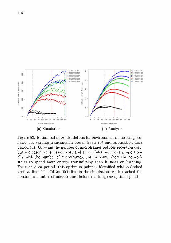
116

050

100

150

200

250


Est

imat

ed n

etw

ork

lifet

ime

(day

s)

●

●●

●●

●●●●●●●●●●

●

●

●●●●●●●●●●●●●●●●●●

●●●

●

●

●

●

●

●

●●

●

●●

●●

●●

●●

●●●

●●●

●●●●●

●●

●●

●●●●●●

●●

●●

●●●●

●●

●●

●

●

●

●

●

●

●

●

●

●

●

●●

●●

●

●●

●●●

●●●

●●●

●●●

●●

●●

●

●●

●●

●●

●●

●

●●

●●

●

●

●●

●

●

●

●

●

●

●

●

●

●

●

●

●

●●

●●

●●

●

●●

●●

●●●

●●

●●●

●

●

●●●

●●●●

●●

●●

●●

●●

●

●

●

●

●

●


5 30 55 80 105 130 155 180 205 230 255

(a) Simulation

050

100

150

200

250


Est

imat

ed n

etw

ork

lifet

ime

(day

s)

●

●●

●●

●●

●●

●●●●●●●●●●●●●●●●●●●●●●●●●●●●●●●●

●

●

●

●

●

●

●

●

●

●

●

●●

●●

●●

●●

●●

●●●●●●●●●●●●●●●●●●●●●●●●●●●●●●

●

●

●

●

●

●

●

●

●

●

●

●

●

●

●

●

●

●●

●●

●●

●●

●●

●●

●●●●●●●●●●●●●●●●●●●●●●

●

●

●

●

●

●

●

●

●

●

●

●

●

●

●

●

●

●

●

●

●

●●

●●

●●

●●

●●

●●

●●●●●●●●●●●●●●●●●●

●

●

●

●


5 30 55 80 105 130 155 180 205 230 255

(b) Analytic

Figure 53: Estimated network lifetime for environment monitoring sce-nario, for varying transmission power levels (p) and application dataperiod (d). Growing the number of microframes reduces reception cost,but increases transmission cost and time. Lifetime grows proportion-ally with the number of microframes, until a point where the networkstarts to spend more energy transmitting than it saves on listening.For each data period, this optimum point is identi�ed with a dashedvertical line. The 7dBm 900s line in the simulation result reached themaximum number of microframes before reaching the optimal point.

117

2930

3132

33


Est

imat

ed n

etw

ork

lifet

ime

(day

s)

31 33 35 37 39 41 43 45 47 49

d = 60s

(a) Network lifetime

0.12

0.14

0.16

0.18

0.20

0.22

0.24


Mea

n la

tenc

y (s

)

31 33 35 37 39 41 43 45 47 49

d = 60s

(b) Mean latency

Figure 54: Estimated network lifetime and mean latency for selectedcon�gurations close to the optimum point of environment monitoringscenario, p=7dBm, d=60s. The optimum network lifetime point isidenti�ed as 43 microframes.

data period with which applications start generating periodic messages;the random backo�s and silence periods in the MAC (Section 3.5.1);channel e�ects on the radio signal; and the clock frequency error foreach node.

118

126

128

130

132

134

136

138


Est

imat

ed n

etw

ork

lifet

ime

(day

s)

156 158 160 162 164 166 168 170 172 174

d = 300s


0.34

0.36

0.38

0.40

0.42


Mea

n la

tenc

y (s

)156 158 160 162 164 166 168 170 172 174

d = 300s

(b) Mean latency


195

200

205

210

215


Est

imat

ed n

etw

ork

lifet

ime

(day

s)

236 238 240 242 244 246 248 250 252 254

d = 600s


0.50

0.52

0.54

0.56

0.58


Mea

n la

tenc

y (s

)

236 238 240 242 244 246 248 250 252 254

d = 600s

(b) Mean latency


119

250

255

260

265

270

275


Est

imat

ed n

etw

ork

lifet

ime

(day

s)

236 238 240 242 244 246 248 250 252 254

d = 900s


0.50

0.52

0.54

0.56

0.58


Mea

n la

tenc

y (s

)

236 238 240 242 244 246 248 250 252 254

d = 900s

(b) Mean latency

Figure 57: Estimated network lifetime and mean latency for selectedcon�gurations close to the optimum point of environment monitoringscenario, p=7dBm, d=900s. The optimum network lifetime point wouldbe beyond 255 microframes.

120

The selected best con�gurations in terms of network lifetime forthe environment monitoring scenario are summarized in Table 10.

Variable UnitData period s 60 300 600 900Nodes - 116 116 116 116TX power dBm 7 7 7 7Microframes - 43 168 253 255MAC period ms 29.51 116.01 174.83 176.21Delivery ratio % 100 100 100 100Network life days 31.6 134.48 209.88 264.5Nominal d.c. % 4.25 1.08 0.72 0.71E�ective d.c. % 5.54 1.36 0.89 0.83Max latency ms 2683.76 2411.74 3015.62 2316.98Mean latency ms 180.27 382.16 565.54 562.11

Table 10: Selected con�gurations for each environment monitoring sce-nario.

4.4.2.2 LISHA O�ce Scenario

The two o�ce scenarios model smaller networks than in environ-ment monitoring, but that are subject to a lossy channel, higher datarates and stricter timing requirements. In both variations, the datageneration period is �xed across simulations, and nodes are not homo-geneous. 60% of the sensor nodes are modeled as nodes that measurenon-critical environmental information, generating one message every10 seconds, with a 10 second expiry. From these, half are battery-powered and half are mains-powered. 20% of the nodes generate datawith higher granularity, every 1 second with 1 second expiry, and aremains-powered. 10% of the nodes measure data at a high rate, every300ms, with equal expiry, and are mains-powered. The 10% remainingnodes represent sensors used for human interaction, sparsely generatingdata (every 1 minute) with a short expiry (300ms), and are battery-powered. To reach higher lifetimes, the battery-powered nodes do notact as forwarders, they only transmit either data messages generated bythemselves, or responses to Keep Alives (Section 3.4.2). Table 11 sum-marizes the con�gurations for the LISHA o�ce scenario, and Figure 58shows the node map.

The same experiments shown in Section 4.4.2.1 are performed for

121


Data rate (λ) 8.05Synchronization period 12s

TX power (p) 0dBm 7dBmRadio range 18m 35m

Avg. # of hops (H) 1 1Avg. # of neighbors (η) 12 12TX power consumption 72mW 102mW

Node con�gurationsNodes with this con�g. 1 1 4 4 3Data period (d) 60s 0.3s 1s 10s 10sData expiry 0.3s 0.3s 1s 10s 10sBattery-powered Yes No No No YesActs as forwarder No Yes Yes Yes No

Table 11: Con�gurations for LISHA o�ce scenario.

●●●●●●●

●

●

●

●

●

●

●

0 2 4 6

01

23

4

X coordinate (m)

Y c

oord

inat

e (m

)

Figure 58: O�ce LISHA node map. Darker shades indicate higher dataperiods. The sink is at the rightmost cluster of nodes, marked with anX.

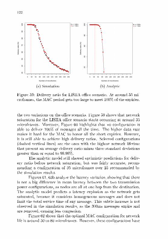
122

3040

5060

7080

9010

0


Del

iver

y ra

tio (

%)

●●●●●●●●●●

●

●●

●

●

●

●

●

●

●

●●●

●

●●

●

●●

●●●●

●●●●

●●

●●●●●

●●

●●●●●

●

p = 0dBmp = 7dBm

5 30 55 80 105 130 155 180 205 230 255

(a) Simulation20

4060

8010

0

Number of microframesD

eliv

ery

ratio

(%

)

●●●●●●●●●●●●●

●

●

●

●

●

●

p = 0dBmp = 7dBm

5 30 55 80 105 130 155 180 205 230 255

(b) Analytic

Figure 59: Delivery ratio for LISHA o�ce scenario. At around 35 mi-croframes, the MAC period gets too large to meet 100% of the expiries.

the two variations on the o�ce scenario. Figure 59 shows that networksaturation for the LISHA o�ce scenario starts occurring at around 35microframes. Moreover, Figure 60 highlights that no con�guration isable to deliver 100% of messages all the time. The higher data ratemakes it hard for the MAC to honor all the short expiries. However,it is still able to achieve high delivery ratios. Selected con�gurations(dashed vertical lines) are the ones with the highest network lifetimethat present an average delivery ratio minus three standard deviationsgreater than or equal to 99.99%.

The analytic model still showed optimistic predictions for deliv-ery ratio before network saturation, but was fairly accurate, recom-mending a con�guration of 35 microframes over 25 recommended bythe simulation results.

Figures 61, 63b analyze the latency variation, showing that thereis not a big di�erence in mean latency between the two transmissionpower con�gurations, as nodes are all at one hop from the destination.The analytic model predicts a latency explosion as the network getssaturated, because it considers homogeneous messages and does notlimit the total service time of any message. This subtle increase is notobserved in the simulation results, as the 300ms messages expire andare removed, causing less congestion.

Figure 62 shows that the optimal MAC con�guration for networklife is around 50 to 80 microframes. However, these con�gurations have

123

99.8

899

.90

99.9

299

.94

99.9

699

.98

100.

00


Del

iver

y ra

tio (

%)

● ● ● ●●

●●

●

●

●

●

●

●

●

●

p = 0dBmp = 7dBm

16 17 18 19 20 21 22 23 24 25 26 27 28 29

Figure 60: Delivery ratio for selected con�gurations of LISHA o�ce sce-nario. In no con�guration the MAC is able to deliver 100% of the mes-sages. 21 microframes with p=7dBm is the largest microframe countwhere it reliably delivers more than 99.99% of messages in time.

0.0

0.2

0.4

0.6

0.8


Mea

n la

tenc

y (s

)

●●●●●

●●

●

●●●

●●

●

●

●●

●●●

●

●

●

●●

●●

●

●

●●

●

●

●

●●

●

●●●

●

●

●

●

●

●●

●●●

●●

p = 0dBmp = 7dBm

5 30 55 80 105 130 155 180 205 230 255

(a) Simulation

02

46

810

1214


Mea

n la

tenc

y (s

)

●●●●●●●●●●●●●●●

●

●

●●

p = 0dBmp = 7dBm

5 30 55 80 105 130 155 180 205 230 255

(b) Analytic

Figure 61: Mean latency for LISHA o�ce scenario. Analytic predic-tions work better for non-saturated networks. The steep increase inlatency is not observed in the simulations, as the analytic model doesnot consider dropping expired messages.

124

2040

6080


Est

imat

ed n

etw

ork

lifet

ime

(day

s)

●

●

●

●

●

●

●

●

●

●

●

●

●

●

●

●

●

●

●

●

●●

●

●

●

●●●

●

●

●

●

●

●

●

●

●

●

●

●●

●

●

●

●

●

●

●

●

●

●

●

p = 0dBmp = 7dBm

5 30 55 80 105 130 155 180 205 230 255

(a) Simulation10

1520

2530

3540

Number of microframesE

stim

ated

net

wor

k lif

etim

e (d

ays)

●

●

●

●

●

●

●

●

●

●

●●

●●●●●●

●

p = 0dBmp = 7dBm

5 30 55 80 105 130 155 180 205 230 255

(b) Analytic

Figure 62: Estimated network lifetime for LISHA o�ce scenario. Theoptimum point is around 50 to 80 microframes.

a low delivery ratio (Figure 59), so Figure 63 considers 16 to 30 mi-croframes. Although 7dBm presents a smaller lifetime when comparedto the same MAC period at 0dBm, it achieves a slightly better deliv-ery ratio, allowing the increase of the number of microframes slightlybeyond what 0dBm supports for the same delivery ratio. The ana-lytic model captures the lifetime behavior, but is pessimistic because itconsiders that all nodes are battery powered and act as forwarders.

The selected con�guration for the LISHA o�ce scenario is sum-marized in Table 13.

125

3035

4045

5055


Est

imat

ed n

etw

ork

lifet

ime

(day

s)

●

●

●

●

●

●

●

●

●

●

●

●

●

●

●

p = 0dBmp = 7dBm

16 17 18 19 20 21 22 23 24 25 26 27 28 29


0.02

50.

030

0.03

50.

040

0.04

5


Mea

n la

tenc

y (s

)

●

●

●

●

●

●

●

●

● ●

●

●●

●●

p = 0dBmp = 7dBm

16 17 18 19 20 21 22 23 24 25 26 27 28 29

(b) Mean latency

Figure 63: Estimated network lifetime and mean latency for selectedcon�gurations of LISHA o�ce scenario. Before reaching the optimumpoint, lifetime grows linearly.

126


Data rate (λ) 22.35Synchronization period 12s

TX power (p) 0dBm 7dBmRadio range 18m 35m

Avg. # of hops (H) 1.154 1Avg. # of neighbors (η) 24.513 37.128TX power consumption 72mW 102mW

Node con�gurationsNodes with this con�g. 3 3 10 12 11Data period (d) 60s 0.3s 1s 10s 10sData expiry 0.3s 0.3s 1s 10s 10sBattery-powered Yes No No No YesActs as forwarder No Yes Yes Yes No

Table 12: Con�gurations for SSB o�ce scenario.

4.4.2.3 SSB O�ce Scenario

The SSB o�ce network has similar parameters to the LISHAvariation, but with more nodes deployed over a larger area, and a higheroverall data rate. Its con�gurations are shown in Table 12, and the nodemap is shown in Figure 64.

Figure 65 shows that TSTP is not able to achieve 100% or even99.99% of delivery ratio in any con�guration. Therefore, the selectedcon�guration is the one that achieves the highest delivery ratio, evenat the cost of lifetime (Figure 66). The analytic model did not produceany valid result, as it �nds the network saturated with messages inevery MAC con�guration.

The selected best con�gurations for both o�ce scenarios are sum-marized in Table 13. The con�gurations shown in Tables 10 and 13 areused for the experiments in Sections 4.4.3 and 4.4.4.

127

●●●●

●●●

●●●

●●

●

●

● ● ●

●●

●●

●●

●

●

●

●

●

●●●

●●●

●●●●

●●

0 5 10 15 20 25 30

010

2030

X coordinate (m)

Y c

oord

inat

e (m

)

Figure 64: O�ce SSB node map. Darker shades indicate higher dataperiods. The sink is marked with an X.

2040

6080

100


Del

iver

y ra

tio (

%)

●

●

●

●

●

●

●

●

●

●

● ●

●

● ●● ●

●●

● ●●

●

p = 0dBmp = 7dBm

5 30 55 80 105

(a) Coarse microframe steps

8890

9294

9698

100


Del

iver

y ra

tio (

%)

●

●

●

●

●●

●

●

●

●

●

p = 0dBmp = 7dBm

6 7 8 9 10 11 12 13 14 15

(b) Granular microframe steps

Figure 65: Delivery ratio for SSB o�ce scenario. (a) At 5 microframes,the MAC contention period is too small, leading to too many collisionsand a drop in delivery ratio. At 10 microframes, it gets the closestto 100%, and falls from 15 and higher. So the best con�guration fordelivery ratio must be in the interval [6,14] microframes. (b) The bestdelivery ratio is at p=7dBm and 6 microframes.

128

2030

4050

6070


Est

imat

ed n

etw

ork

lifet

ime

(day

s)

●

●

●

●

●

●● ●

●

●

●

●

●

● ●● ●

●

●

●●

●

●

p = 0dBmp = 7dBm

5 30 55 80 105


1520

2530

3540

45


Est

imat

ed n

etw

ork

lifet

ime

(day

s)●

●

●

●

●

●

●

●

●

●●

p = 0dBmp = 7dBm

6 7 8 9 10 11 12 13 14 15


Figure 66: Estimated network lifetime for SSB o�ce scenario. Higherlifetime can be achieved, but only with a signi�cant decrease in deliveryratio.

0.2

0.4

0.6

0.8

1.0


Mea

n la

tenc

y (s

)

●

●

●

●

●

●

● ●

●

●

●● ●

●

●

●

●

●

●●

●

●

●

p = 0dBmp = 7dBm

5 30 55 80 105


0.04

0.06

0.08

0.10

0.12


Mea

n la

tenc

y (s

)

●

●

●

●●

●●

●

●

●

●

p = 0dBmp = 7dBm

6 7 8 9 10 11 12 13 14 15


Figure 67: Mean latency for SSB o�ce scenario. At 5 microframes, theshort MAC contention period leads to signi�cantly more collisions andan increase in latency.

129

Variable UnitNode map - LISHA SSBNodes - 14 40TX power dBm 7 7Microframes - 21 6MAC period ms 14.28 3.90Delivery ratio % 99.99 99.59Network life days 40.08 15.27Nominal d.c. % 8.78 32.09E�ective d.c. % 10.79 27.38Max latency ms 495.67 1268.98Mean latency ms 33.05 24.85

Table 13: Selected con�gurations for each o�ce scenario.

130

4.4.3 Synchronization

The following set of simulations investigates the e�ectiveness ofthe employment of speculative synchronization techniques such as theSpeculative Precision Time Protocol (Sections 2.4, 3.4) in TSTP. To al-low nodes to synchronize only by overhearing passing messages, TSTPincludes in the common message header (Figure 17) of every messagesynchronization information such as the precise time of message trans-mission. This increases the size of every message, but reduces theoverall number of messages if compared to an approach that sends syn-chronization information only in periodic messages commonly known asbeacons. The speculative approach should save energy in most cases, assending a new message is much more energy-consuming than includingextra bytes in a message that would already be sent, because new mes-sages come with MAC preambles, contention, potential collisions, extraheaders, etc. However, depending on the proportion of synchronizationbeacons and data messages, there may be cases where explicit synchro-nization approaches perform better. The following set of experimentsanalyzes if, and under which circunstances, is it better to pigtail tim-ing information to every message, compared to only exchanging timinginformation in periodic beacons.

The experiments that follow use the same scenario parameterspresented in Tables 9, 11, 12, with the identi�ed optimal MAC pream-ble and radio transmission power con�gurations shown in Tables 10,13. The analyzed input variable is the SPTP maximum tolerable syn-chronization period P (Section 3.4.2), which was �xed in the priorsimulations. The impact of this parameter on delivery ratio, latency,network lifetime, and average clock synchronization accuracy is eval-uated. Each experiment runs for 2 hours of simulated time, and isreplicated 20 times. Shaded areas in the �gures represent standarddeviations among the means of the 20 replications. For the o�ce sce-narios, the considered synchronization periods are 240s, 200s, 160s,140s, 120s, 100s, 80s, 60s, 40s, 30s, 20s, 10s, 5s. For the environmentmonitoring scenarios, the considered synchronization periods are 3600s,2700s, 2400s, 1800s, 1200s, 900s, 600s, 480s, 300s, 240s, 180s, 120s, 60s,30s, 15s.

TSTP performance (Speculative) is compared with a theoret-ical and an explicit strategies. The Theoretical data are calculationsconsidering that timestamps are not embedded in every message, buttransmitted once per half synchronization period per node. It considersperfect channel conditions with no collisions, representing an approx-

131

imation of what any explicit synchronization protocol with a similarstrategy could achieve2. The Explicit strategy is a variation on TSTPthat implements the theoretical approach: it does not include times-tamps in the common message header (making it smaller), but only inKeep Alive messages (making them potentially more frequent).

Clock synchronization accuracy is measured once per simulatedsecond by taking the absolute di�erence between each node's currenttimestamp and the sink's.

4.4.3.1 LISHA O�ce Scenario

Figure 68 presents the impact of the synchronization period ondelivery ratio. Lower synchronization periods decrease delivery ratio, asmore Keep Alive messages are sent. The speculative approach showsa generally higher standard deviation, since depending on the environ-ment a node might need to send more or less explicit synchronizationmessages, whereas for Explicit the number of Keep Alives only de-pends on the synchronization period. As the period increases, thenumber of explicit messages decreases in both approaches, and theybecome more similar. Latency (Figure 69) shows a similar behavior,for the same reasons.

The number of Keep Alive messages sent are shown in Fig-ure 70. As expected, the number of explicit synchronization messagesfor each strategy converges as the synchronization period increases,and the speculative approach reaches zero as the synchronization pe-riod gets larger than twice the maximum application data period of60s. The explicit approach sends more synchronization messages thanthe theoretical, as the latter considers a perfect network with one syn-chronization message per node per half period, with no collisions.

Figure 71 shows the average clock error between sensor nodesand the sink. Clock synchronization accuracy is measured once persimulated second by taking the absolute di�erence between each node'scurrent timestamp and the sink's. In this case, the �Theoretical� lineshows the expected clock error to occur in the expected time elapsedbetween two synchronization messages, assuming that synchronization

2It is not meant to be an absolute best case, but a comparable approach withgood performance. A protocol could achieve better performance than the Theo-retical approach, as it considers that every node sends synchronization beacons atevery half period.

132

99.5

99.6

99.7

99.8

99.9

100.

0

Synchronization period (s)

Del

iver

y ra

tio (

%) ●

●

●

●

●●

●

● ●

● ● ●●

●

SpeculativeExplicit

0 30 60 90 120 150 180 210 240

Figure 68: Delivery ratio for LISHA o�ce scenario, p=7dBm, 21 mi-croframes, varying synchronization period. Comparison between TSTP(Speculative), and a TSTP version that does not include timestampsin the header and will only synchronize with explicit keep alives (Ex-plicit). Higher synchronization periods lead to less explicit messages,so delivery ratio grows. As the synchronization period grows, bothapproaches converge, since there will be fewer keep alives.

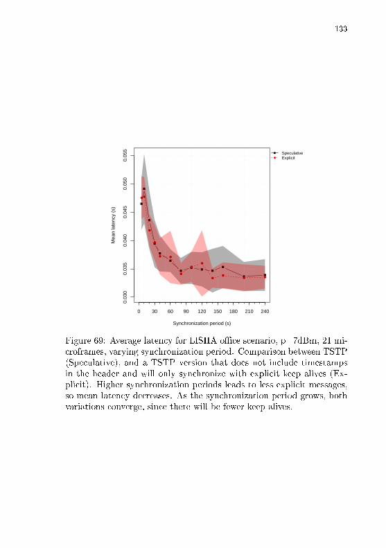
133

0.03

00.

035

0.04

00.

045

0.05

00.

055


Mea

n la

tenc

y (s

)

●●

●

●

● ●

●

●●

●●

● ●

●

SpeculativeExplicit

0 30 60 90 120 150 180 210 240

Figure 69: Average latency for LISHA o�ce scenario, p=7dBm, 21 mi-croframes, varying synchronization period. Comparison between TSTP(Speculative), and a TSTP version that does not include timestampsin the header and will only synchronize with explicit keep alives (Ex-plicit). Higher synchronization periods leads to less explicit messages,so mean latency decreases. As the synchronization period grows, bothvariations converge, since there will be fewer keep alives.

134

010

000

2000

030

000

4000

050

000

6000

070

000


Kee

paliv

es s

ent

●

●

●

●●

●

●●

●●

● ● ●

●

SpeculativeExplicitTheoretical

0 30 60 90 120 150 180 210 240

Figure 70: Number of explicit synchronization messages for LISHAo�ce scenario. �Theoretical� is one keep alive per node per synchro-nization half period. �Explicit� sends more keep alives due to imperfectchannel conditions. �Speculative� sends less because it uses regulardata messages as synchronization messages most of the time. At peri-ods greater than 140s, Speculative reaches zero explicit synchronizationmessages.

135

messages arrive at every node with a period PS :

PS = min(SP /2, d) (4.6)

where SP is the synchronization period, and d is the average applicationdata period (12s for the o�ce scenarios). Theoretical clock drifts aregenerated in the same way as Castalia computes clock frequency errors.This bound applies only to the speculative strategy, as the explicit onetriggers synchronization messages only every SP /2 time, and the clockerror upper bound grows proportionally to the synchronization period.

The average clock error for both approaches is below the calcu-lated upper bound, indicating that SPTP's frequency error correction(Section 2.4) is e�ective. As the synchronization period increases, thespeculative approach is expected to achieve better clock synchroniza-tion than the explicit strategy, because it uses timestamps from regulardata messages in addition to the ones in Keep Alive messages. Thedata shows that the di�erence is not big in this scenario, however. Italso shows that the speculative clock error decreases with higher syn-chronization periods, which can be explained by the higher deliveryratio achieved in such cases: the network is less saturated, so nodescan actually get timestamps without collisions more often.

The analyses so far indicate that there is not a big di�erencein terms of latency, clock error, or delivery ratio between the explicitand speculative approaches for the LISHA o�ce scenario. As Figure 70shows, the speculative approach saves a considerable number of KeepAlive messages. However, regular data messages are bigger in thespeculative approach, as they include timestamps, so an energy analysisis necessary to determine whether the savings in number of messagesis bigger than the cost of pigtailing timestamps.

Figure 72 compares the energy consumption of both strategieswith the theoretical approach. At low synchronization periods, thespeculative approach is able to save a proportionally large number ofKeep Alive messages, and performs much better in terms of energy.As the proportion of synchronization messages decrease in relation todata messages, the cost of pigtailing timestamps to data messages isproportionally bigger, and the speculative approach performs compara-tively worse. At a synchronization period of around 90s, the theoreticalapproach starts saving more energy than the speculative one. However,the explicit strategy, which is an implementation of the theoretical ap-proach subjected to similar network conditions, shows that the spec-ulative strategy saves more energy for all synchronization periods up

136

050

100

150

200


Ave

rage

clo

ck e

rror

(us

)

●

●

●

●

●

●

●

●

●

●

●

●

●

●


0 30 60 90 120 150 180 210 240

Figure 71: Average clock error for LISHA o�ce scenario. Clock errorshould be inversely proportional to synchronization period. However,as the synchronization period grows, delivery ratio also grows, and thisindicates that nodes are able to access more synchronization messagesmore often, so clock error is actually lower at higher synchronizationperiods. For periods >160s (for Speculative) and >200s (for Explicit),delivery ratio stabilizes and clock error grows according to the syncperiod.

137

−10

000

010

000

2000

030

000


The

oret

ical

ene

rgy

gain

(J)

●

●

● ● ●●

●●

●●

● ● ●

●

SpeculativeExplicit

0 30 60 90 120 150 180 210 240

Figure 72: Energy consumption compared to theoretical explicit ap-proach for LISHA o�ce scenario. Theoretical energy gain is calculatedcomparing the cost of including timestamps in every message to thesavings in number of explicit synchronization messages.

to 240s (four times the maximum application data period, 60s). Fig-ure 73 shows the estimated network lifetime for both implementations,con�rming that the speculative approach saves signi�cant amounts ofenergy in every case.

4.4.3.2 SSB O�ce Scenario

The SSB o�ce scenario features more nodes and hops than theLISHA scenario, with a high data rate that puts the network over itslimit. Figures 74 and 75 show that the speculative approach performsslightly better than the explicit approach in terms of delivery ratio andlatency. Delivery ratio increases and average latency decreases for bothimplementations as the synchronization period gets bigger.

The number of Keep Alives sent, shown in Figure 76, showsthe same behavior as in the LISHA scenario. The average clock error(Figure 77) is slightly better for the speculative implementation, as thedenser network deployment allows nodes to receive data messages more

138

3035

4045

50


Est

imat

ed n

etw

ork

lifet

ime

(day

s)

●

●

●

●

● ●●

●

●

●

●

● ●

●

SpeculativeExplicit

0 30 60 90 120 150 180 210 240

Figure 73: Estimated network lifetime for LISHA o�ce scenario. TheSpeculative approach saves energy signi�catively.

8890

9294

9698

100


Del

iver

y ra

tio (

%)

●●

●

●

●

●

●●

●●

●● ●

●

SpeculativeExplicit

0 30 60 90 120 150 180 210 240

Figure 74: Delivery ratio for SSB o�ce scenario, with p=7dBm and 6microframes. Similarly to the LISHA variation, delivery ratio grows asless synchronization messages are generated.

139

0.02

0.04

0.06

0.08

0.10

0.12


Mea

n la

tenc

y (s

)

●●

●

●

●

●

●

●●

● ●● ●

●

SpeculativeExplicit

0 30 60 90 120 150 180 210 240

Figure 75: Average latency for SSB o�ce scenario. Similarly to theLISHA variation, latency decreases as less synchronization messagesare generated.

frequently.Figure 78 shows that a theoretical implementation could reach

lower overall energy consumption starting from a synchronization pe-riod of around 10 seconds. However, in practice, the explicit implemen-tation still spends more energy on explicit synchronization messagesthan it saves in not including timestamps in the common header. Fig-ure 79 shows that this energy di�erence leads to a very small variationin the estimated network lifetime, possibly because the battery-powerednodes are not particularly bene�ted from the energy savings.

140

050

000

1000

0015

0000


Kee

paliv

es s

ent

●

●

●

●

●

●

● ● ● ●● ● ●

●


0 30 60 90 120 150 180 210 240

Figure 76: Number of explicit synchronization messages for SSB o�cescenario. �Theoretical� is one keep alive per node per half synchroniza-tion period. �Explicit� sends more keep alives due to imperfect channelconditions. �Speculative� sends less because it uses regular data mes-sages as synchronization messages most of the time. At periods greaterthan 140s, Speculative reaches zero explicit synchronization messages.

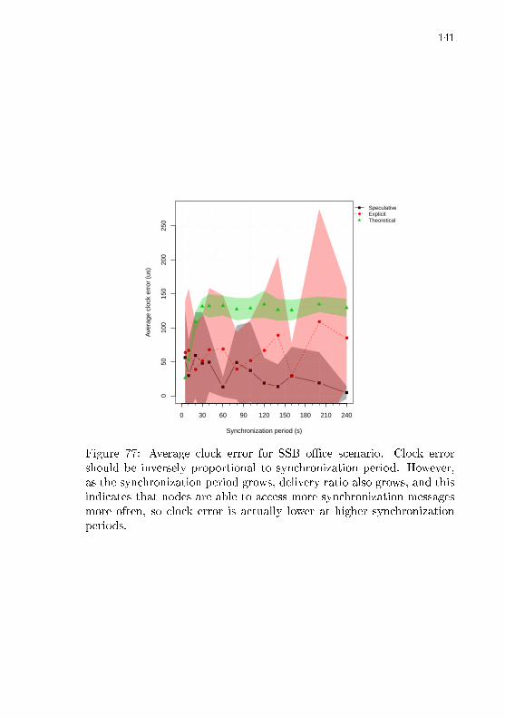
141

050

100

150

200

250


Ave

rage

clo

ck e

rror

(us

)

●●

●

●

● ●

●

●

●

●

●

●

●

●


0 30 60 90 120 150 180 210 240

Figure 77: Average clock error for SSB o�ce scenario. Clock errorshould be inversely proportional to synchronization period. However,as the synchronization period grows, delivery ratio also grows, and thisindicates that nodes are able to access more synchronization messagesmore often, so clock error is actually lower at higher synchronizationperiods.

142

−15

000

−50

000

5000

1000

015

000

2000

0


The

oret

ical

ene

rgy

gain

(J)

●

●

●

● ●●

● ● ● ●● ● ●

●

SpeculativeExplicit

0 30 60 90 120 150 180 210 240

Figure 78: Energy consumption compared to theoretical explicit ap-proach for SSB o�ce scenario. Theoretical energy gain is calculatedcomparing the cost of including timestamps in every message to thesavings in number of explicit synchronization messages. The theoreti-cal approach quickly outperforms the speculative, which is still betterthan �Explicit�, an implementation of the theoretical approach mea-sured under the same conditions as �Speculative�.

143

1618

2022


Est

imat

ed n

etw

ork

lifet

ime

(day

s)

●

●

●

●

●

●

●

●●

● ● ● ●

●

SpeculativeExplicit

0 30 60 90 120 150 180 210 240

Figure 79: Estimated network lifetime for SSB o�ce scenario. Bothapproaches show similar results.

144

In the LISHA o�ce scenario, the speculative and explicit ap-proaches perform very close in terms of overall clock error, latency, anddelivery ratio, but the speculative approach shows signi�cantly lowerenergy consumption. In the SSB scenario where the network is satu-rated, the speculative approach performs only slightly better, but doesso for every measured metric.

4.4.3.3 Environment Monitoring Scenario

For better visualization, the graphics that follow are divided intwo: low synchronization periods, up to 2d (where d is the applicationdata period), and high synchronization periods, from d up to 6d. Thedashed vertical lines mark the point in the x axis where the synchro-nization period is equal to the data period. Data periods of 60s and600s are considered in this section. The results for the periods of 300sand 900s show similar behavior to the 600s ones, and can be found inSection A.1 in the Appendix.

The environment monitoring scenario is a more regular one thanboth o�ce scenarios. The network is larger, node deployment is uni-form, and tra�c is sparser, which makes the predictions of the theo-retical approach more accurate. Figures 80, 81 show that indeed thenumber of synchronization messages sent by the explicit approach isclose to one per node per half period (the �Theoretical� line). Thespeculative approach generally saves a large number of explicit mes-sages, unless the synchronization period is much lower than the dataperiod, in which case there are not enough data messages to serve assynchronization messages. Figure 81a shows that this only starts hap-pening when the synchronization period falls below around d/20.

Latency is expected to start lower with the speculative approach,as it is able to send less messages than the explicit one. However, theincrease in data message size caused by the inclusion of timestampseventually leads to a slightly higher latency, as the synchronization pe-riod gets higher and the network produces much more data messagesthan synchronization messages. Figures 82, 83 show that the synchro-nization period needs to be around 5 times the data period for theexplicit approach to start showing slightly better latencies.

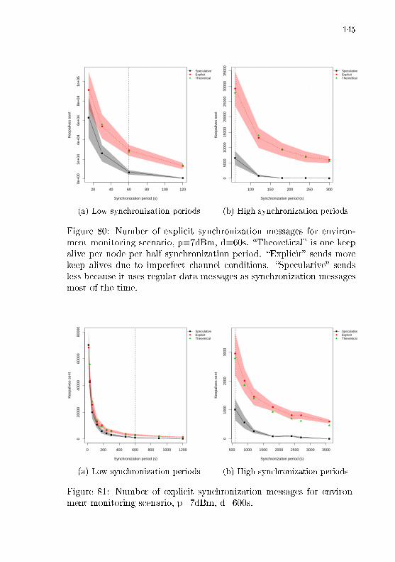
145

20 40 60 80 100 120

0e+

002e

+04

4e+

046e

+04

8e+

041e

+05


Kee

paliv

es s

ent

●

●

●

●

●


(a) Low synchronization periods

100 150 200 250 300

050

0010

000

1500

020

000

2500

030

000

3500

0


Kee

paliv

es s

ent

●

●

●

●

●

●


(b) High synchronization periods

Figure 80: Number of explicit synchronization messages for environ-ment monitoring scenario, p=7dBm, d=60s. �Theoretical� is one keepalive per node per half synchronization period. �Explicit� sends morekeep alives due to imperfect channel conditions. �Speculative� sendsless because it uses regular data messages as synchronization messagesmost of the time.

0 200 400 600 800 1000 1200

020

000

4000

060

000

8000

0


Kee

paliv

es s

ent

●

●

●

●

●

● ●

● ●● ●

●



500 1000 1500 2000 2500 3000 3500

010

0020

0030

00


Kee

paliv

es s

ent

●

●

●

●

● ●

●

●



Figure 81: Number of explicit synchronization messages for environ-ment monitoring scenario, p=7dBm, d=600s.

146

20 40 60 80 100 120

0.17

0.18

0.19

0.20

0.21

0.22


Mea

n la

tenc

y (s

)

●

●

●

●

●

SpeculativeExplicit


100 150 200 250 3000.

170.

180.

190.

20


Mea

n la

tenc

y (s

)

●

●

●

●

●

●

SpeculativeExplicit


Figure 82: Average latency for environment monitoring scenario,d=60s. Only at synchronization periods of 300s the Explicit approachreaches a slightly better average.

0 200 400 600 800 1000 1200

0.6

0.7

0.8

0.9

1.0

1.1


Mea

n la

tenc

y (s

)

●

●

●

●

●

● ●

● ●●

●

●

SpeculativeExplicit


500 1000 1500 2000 2500 3000 3500

0.54

0.56

0.58

0.60


Mea

n la

tenc

y (s

)

●

●

●

● ● ●

●

●

SpeculativeExplicit


Figure 83: Average latency for environment monitoring scenario,d=600s. Only at synchronization periods of 3600s the Explicit ap-proach reaches a slightly better average.

147

20 40 60 80 100 120

010

020

030

040

050

060

070

0


Ave

rage

clo

ck e

rror

(us

)

●

● ●●

●



100 150 200 250 300

010

020

030

040

050

060

070

0


Ave

rage

clo

ck e

rror

(us

)

●●

●

●

●

●



Figure 84: Average clock error for environment monitoring scenario,d=60s.

Increasing the synchronization period, however, necessarily in-creases the overall clock error for the explicit strategy. Figures 84 and85 show that both strategies are roughly equally e�ective at synchro-nizing the clocks. However, with synchronization periods greater than1500s, the explicit approach starts to wildly vary its clock synchroniza-tion e�ectiveness, while the speculative approach maintains constantperformance as the data period remains the same.

Figures 86 and 87 further con�rm that the theoretical estima-tions are more accurate for the environment monitoring scenarios, asthe explicit implementation shows an energy performance close to thetheoretical. The Figures also show that the overall energy consumptionfor the speculative approach is lower in every measurement. Figures 88,89 show that the expected network lifetime for the speculative approachis indeed higher up until synchronization periods of around 5d.

148

0 200 400 600 800 1000 1200

010

0020

0030

0040

0050

0060

00


Ave

rage

clo

ck e

rror

(us

)

●● ● ● ● ●● ●

●

●

●

●



500 1000 1500 2000 2500 3000 35000

5000

1000

015

000

2000

025

000


Ave

rage

clo

ck e

rror

(us

)● ●

●

●

●●

●

●




20 40 60 80 100 120

−20

000

020

000

4000

060

000

8000

010

0000

1200

00


The

oret

ical

ene

rgy

gain

(J)

●

●

●●

●

SpeculativeExplicit


100 150 200 250 300

−10

000

010

000

2000

030

000


The

oret

ical

ene

rgy

gain

(J)

●

●

● ●●

●

SpeculativeExplicit


Figure 86: Energy consumption compared to theoretical explicit ap-proach for environment monitoring scenario, d=60s.

149

0 200 400 600 800 1000 1200

0e+

001e

+05

2e+

053e

+05

4e+

055e

+05


The

oret

ical

ene

rgy

gain

(J)

●

●

●●

●●

● ● ● ● ●

●

SpeculativeExplicit


500 1000 1500 2000 2500 3000 3500

−50

000

5000

1000

015

000


The

oret

ical

ene

rgy

gain

(J)

● ●

●

●●

●●

●

SpeculativeExplicit



150

20 40 60 80 100 120

2728

2930

3132


Est

imat

ed n

etw

ork

lifet

ime

(day

s)

●

●

●

●

●

SpeculativeExplicit


100 150 200 250 300

29.5

30.0

30.5

31.0

31.5

32.0

32.5

Synchronization period (s)E

stim

ated

net

wor

k lif

etim

e (d

ays)

●

●

●

●●

●

SpeculativeExplicit


Figure 88: Estimated network lifetime for environment monitoring sce-nario, d=60s. Only at synchronization periods of 300s the Explicitapproach reaches a slightly better average.

The analyses show that, for the environment monitoring sce-narios, the speculative approach shows better latency and energy con-sumption, and comparable clock error in relation to the explicit syn-chronization approach, which performs close to a theoretical explicitclock synchronization algorithm. When the synchronization period isgreater than �ve times the data period, the burden of including times-tamps in each message starts to show on energy and latency. However,the speculative approach maintains clock synchronization performanceindependent of the synchronization period, and for higher data periodsthe 5d point where the explicit approach becomes better comes withthe cost of a large increase in clock error across the network.

151

0 200 400 600 800 1000 1200

5010

015

020

0


Est

imat

ed n

etw

ork

lifet

ime

(day

s)

●

●

●

●

●

● ●

●

●

●

●

●

SpeculativeExplicit


500 1000 1500 2000 2500 3000 3500

180

190

200

210

220


Est

imat

ed n

etw

ork

lifet

ime

(day

s)

●

●

●

●

●

●

●

●

SpeculativeExplicit


Figure 89: Estimated network lifetime for environment monitoring sce-nario, d=600s. Only at synchronization periods of 3600s the Explicitapproach reaches a slightly better average.

152

4.4.4 Routing Metrics

Equation 2.7 in Section 2.5.1 introduces the concept of the dis-tortion coe�cient α, which is a real number in the interval [0, 1] usedto skew the distance-based contention o�set for message transmissionaccording to any metric of interest. In this section, two such metricsare presented and their overall impact on network performance is eval-uated.

4.4.4.1 Expiry Metric

The Expiry metric de�nes a distortion coe�cient in�uenced byhow much time the message has left to reach its destination. Messagesthat are close to expiring shrink space, reducing the node's o�set δ(m),and providing it a better chance to win the contention and forward thatmessage quickly. Equation 4.7 de�nes the distortion coe�cient for theExpiry metric.

α =Em − tEm

(4.7)

where Em is the timestamp in which message m expires and t is thecurrent time. It is assumed that Em > t, as otherwise m is an expiredmessage that should be dropped. The Expiry metric has been used forall of the simulation experiments presented so far.

4.4.4.2 E�ort Metric

The E�ort metric distorts space based on how much the nodehas cooperated with the network doing message forwarding in the past.The more messages the node has forwarded, the more space is dilated,and the less likely that node becomes to forward again. This metricseeks a balance on the network for neighbors on the same hop fromthe destination to better alternate the e�ort of forwarding messages.Equation 4.8 de�nes the distortion coe�cient for the e�ort metric.

α =Fn

Txn(4.8)

where Fn is the number of queued messages from neighbors that noden has relayed so far, and Txn is the total number of messages that

153

the node has transmitted in the past (including its own generated mes-sages). The e�ort metric takes information from the node's history,rather than from the message being forwarded.

4.4.4.3 Evaluation

The goal of the following experiments is to analyze the e�ec-tiveness of each di�erent routing metric. The metrics are compared tothree other control groups. The Distance metric takes only the dis-tance into account, and is de�ned as Equation 2.7 with a �xed α = 1.Likewise, the Zero metric simply sets α = 0, such that nodes alwayshave the lowest possible o�set, and collision control is fully managedby the MAC's random backo� and silence mechanisms (Section 3.5.1).Random sets every o�set δ to a random number. A combination ofthe Expiry and E�ort metrics is also assessed (the two α values mul-tiplied), and is labeled Expiry E�ort Distance. The Expiry andE�ort metrics are explained in Sections 4.4.4.1 and 4.4.4.2, respec-tively.

The same scenario parameters presented in Tables 9, 11, 12 areused, with the identi�ed optimal MAC preamble and radio transmissionpower con�gurations shown in Tables 10, 13. The varied input variableis the way the α component is calculated during MAC contention.

The statistics measured are network lifetime, average latency,transmission fairness index, and o�set standard deviation. The fairnessindex indicates how balanced was the amount of messages that wererelayed by the nodes, according to Equation 4.9:

FI =(∑F )2

N ×∑

(F 2)(4.9)

where F is the number of message relayed, and N is the number ofnodes. The highest the value of the fairness index, the more nodes al-ternate in forwarding messages, which leads to a better distribution ofthe energy consumption, avoiding a certain routing path to be overusedand prematurely deplete the energy of particular nodes. Because bydesign the sink will normally spend much more energy than any othernode (it needs to acknowledge every message), its message transmis-sion statistics are not included in the fairness index calculation. Theo�set standard deviation indicates how well the metric spreads o�sets,potentially reducing the probability of collisions.

For the SSB o�ce scenario, Figure 90a shows that the rout-

154

Zero

Effort Distance

Expiry Distance

Random

Distance

Expiry Effort Distance

Estimated network lifetime (days)

0 2 4 6 8 10 12 14


Zero

Effort Distance

Distance

Random


Expiry Distance

Mean latency (s)

0.000 0.005 0.010 0.015 0.020 0.025 0.030

(b) Mean latency

Figure 90: Estimated network lifetime and mean latency for SSB o�cescenario under di�erent routing metrics.

ing metrics have little impact on network life. This is expected, asbattery-powered nodes do not forward messages in the o�ce scenarios.Figures 90b and 91a suggest that the variations in latency and fairnessindex are not statistically relevant, as there is a big overlap between allstandard deviation intervals. This happens because SSB is a scenariowith few hops overall, such that routing decisions have little impact.

In the larger environment monitoring scenario, messages need totravel more hops on average, and routing decisions impact network per-formance. Figure 92a shows that the Distance and E�ort metrics yieldthe best network lifetime for a data period of 60s. The Distance metriccalculates larger o�sets in general, which means that nodes spend moretime with their radios o� before transmission. However, for larger dataperiods, the con�gured MAC contention period that limits the o�setsis increased (Table 10), and the routing metrics have more room tovary the o�set without causing collisions. Figure 94a shows that ford = 600s, the E�ort metric performs the best in terms of networklifetime. It is the only metric that signi�cantly outperforms Random,which also achieves a balancing in forwarder selection. As expected,the Zero metric shows a comparatively bad network lifetime, as it ismore likely to cause collisions and retransmissions. The fact that bothExpiry metrics are close to the Zero metric for d=60s and close to theRandom metric in d=600s further indicates that the MAC period of29.51ms is too short for these metrics, generating more collisions.

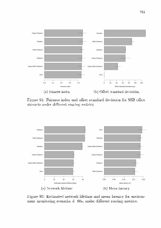
155

Zero


Distance

Effort Distance

Random

Expiry Distance

Fairness Index

0.0 0.1 0.2 0.3 0.4

(a) Fainess index

Zero


Expiry Distance

Distance

Effort Distance

Random

Offset Standard Deviation (µs)

0 20 40 60 80 100 120

(b) O�set standard deviation

Figure 91: Fairness index and o�set standard deviation for SSB o�cescenario under di�erent routing metrics.

Zero


Expiry Distance

Random

Effort Distance

Distance


0 10 20 30 40


Effort Distance

Distance

Expiry Distance


Random

Zero

Mean latency (s)

0.00 0.05 0.10 0.15 0.20

(b) Mean latency

Figure 92: Estimated network lifetime and mean latency for environ-ment monitoring scenario, d=60s, under di�erent routing metrics.

156

Distance

Expiry Distance

Zero


Effort Distance

Random

Fairness Index

0.0 0.1 0.2 0.3 0.4 0.5 0.6

(a) Fainess index

Zero


Expiry Distance

Effort Distance

Distance

Random


0 1000 2000 3000 4000 5000 6000 7000


Figure 93: Fairness index and o�set standard deviation for environmentmonitoring scenario, d=60s, under di�erent routing metrics.

Zero

Expiry Distance


Distance

Random

Effort Distance


0 50 100 150 200



Expiry Distance

Effort Distance

Distance

Zero

Random

Mean latency (s)

0.0 0.2 0.4 0.6 0.8

(b) Mean latency


157

Expiry Distance

Zero

Distance


Random

Effort Distance

Fairness Index

0.0 0.1 0.2 0.3 0.4 0.5 0.6 0.7

(a) Fainess index

Zero


Expiry Distance

Effort Distance

Distance

Random


0 10000 20000 30000 40000


Figure 95: Fairness index and o�set standard deviation for environmentmonitoring scenario, d=600s, under di�erent routing metrics.

Figures 93a, 95a indicate that the E�ort metric is indeed ableto maintain a high fairness index, comparable to the Random metric.Figure 92b shows that the Distance and E�ort metrics end up havinga lower latency when d=60s, possibly for avoiding collisions more thanthe other metrics. However, for a higher data and MAC period, theExpiry metric signi�cantly reduces the overall latency, as shown inFigure 94b.

No strong correlations were found between the o�set standarddeviations (Figures 91b, 93b, 95b) and other statistics, which indicatesthat a higher spreading of the o�set does not signi�cantly reduce thenumber of collisions in the observed cases.

Results for the LISHA o�ce scenario and environment monitor-ing with d=300s and d=900s are similar to SSB and d=600s, and canbe found in Section A.2 of the Appendix.

Overall, the Expiry metric performs better in terms of latencyand only slightly worse in terms of network lifetime than the E�ortmetric. However, for smaller MAC periods, the E�ort metric is ableto prevent more collisions and balance the tra�c better, performingbetter even in terms of latency.

158

4.5 EVALUATION SUMMARY

The main results obtained from the performance evaluations are:

• The code sizes for both implementations of TSTP (simulator andreal-world), including all of its features, is close to two third-partyimplementations of the AODV protocol for the same simulationframework. AODV only implements routing.

• The bu�er handling architecture shows light time overhead. Theaverage time overhead for allocation of zero-copy bu�ers in EPOS-Mote III is 2.31µs. The noti�cation mechanism used for bu�erpropagation accounts for 11.60% of the total bu�er processingtime across the components.

• The code responsible for time synchronization on EPOSMote IIIis time-deterministic. The delay from sending and receiving Start-of-Frame Delimiters (SFD) between two devices has a jitter of93.5ns, including software and radio delays. This leads to a highlyaccurate time synchronization protocol that is able to achieve sub-microsecond instant clock synchronization, as measured on realEPOSMote III devices.

• There is an optimal point on MAC preamble size which dependson network topology and tra�c. By selecting the right MACparameters, large networks are able to achieve e�ective radio dutycycles smaller than 1% while keeping 100% delivery ratio andaverage latencies around 0.5s.

• Including timestamps in every message to enable speculative clocksynchronization is bene�cial in all the scenarios considered whencompared to explicit, beaconed clock synchronization strategies.For small, tra�c-intensive networks, the reduction in number ofmessages leads to an increase in energy e�ciency. For largernetworks with lighter tra�c, the inclusion of timestamps in datamessages slightly improves latencies and energy e�ciency, whilekeeping a better lower bound on clock accuracy.

• When the network is not saturated, the simplistic analytic modelshows similar results to the detailed simulations, while beingmuch faster to execute. It is thus an appropriate �rst step foranalyzing the expected behavior of new network deployments.

159

4.6 DISCUSSION

The MAC currently in use by TSTP, based on RB-MAC, hasmany bene�ts such as low idle listening duty cycles; resiliency to lossylinks due to multiple nodes being able to forward a given message,further improved by the possibility of using multiple channels withno additional overhead (Section 3.5.1); enabling reactive routing andspeculative synchronization; and allowing energy-constrained nodes tosave energy by not acting as forwarders. It also does not impose anyrequirements on clock synchronization accuracy, nor requires schedulingor structuring of the network. However, the analyses show that itsperformance in terms of delivery ratio, energy, and latency, makes itunsuitable depending on the network requirements.

For the environment monitoring scenarios, while a delivery ratioof 100% is achievable for all considered data periods, network lifetimeis generally the most important metric of interest, and as was shown inthe �gures, there is an optimal point imposed by the MAC that is de-pendent on the network and the tra�c. This optimum might reach 264days of full network operation (Table 10) for very sparse tra�c, whichmight be reasonable for some applications, but a lifetime of aroundone month is not impressive for a network with nodes each generatingdata once per minute. What's worse, the analyses show that reducingthe radio transmission power actually decreases network lifetime evenmore, as messages need to travel more hops towards the destination.The literature commonly refers to 1% as the goal for radio duty cycles,and TSTP MAC is only able to achieve 1% at data periods greater than300s for the studied scenarios. Nevertheless, if the granted network life-time is enough for a given application, TSTP achieves reasonably lowand bounded latencies, 100% delivery ratio, and clock synchronizationsof around hundreds of microseconds across the entire network.

For both o�ce scenarios, the situation is worse. The presenceof battery-powered nodes, a noisy environment, higher data rates, andmessage expiration times as low as 300ms make it impossible for theMAC to reliably deliver 100% of the messages in time for the considereddeployments. It seems that this limitation can only be solved by relax-ing application requirements: either allowing a margin of message loss,or reducing the overall data rate. While a tolerable message loss doeslead to signi�cant gains in network lifetime, such a trade-o� betweennetwork life and delivery ratio might not be a reasonable imposition onthe network design.

Many techniques were employed to improve the MAC's perfor-

160

mance (Section 3.5.1), such as switching channels to transmit data mes-sages, making battery-powered nodes not act as forwarders, di�erentbu�er selection criteria on the MAC transmission schedule, or manip-ulating the contention o�sets using di�erent metrics. While some ofthese techniques did in fact improve performance, their result is whatis shown in the analyses of this work. It seems like RB-MAC has beentuned to its limit, and it is still not enough for some real-world appli-cations.

The proposed analytic model (Section 4.3) reproduced the gen-eral behavior of the MAC, but is not RB-MAC speci�c. It considers asimple model of collision resolution and makes few assumptions aboutMAC operation. Namely, it assumes a CSMA/CA model where con-tention access periods of a given duration arrive on a �xed interval ateach node, that only one message can be sent by period (because of thelong preambles), and takes as input the average end-to-end throughputof the MAC. Although the model is optimistic on most of its predic-tions in relation to the observed simulation results, it is not far o�,indicating that the speci�c design and implementation of the MAC arenot the major factors in performance, but rather the general techniquesemployed.

It is an important factor that TSTP as a whole achieves perfor-mance close to the analytic model of the MAC while delivering all ofits higher-level features that directly bene�t applications and program-mers (Section 2.1). It was shown that the implementation techniquesused for TSTP lead to a code size comparable to an implementationof AODV, a routing-only protocol (Section 4.2.1). The mechanismsfor bu�er management impose a low overhead in the architecture (Sec-tion 4.2.2). The clock synchronization algorithm was shown to be e�ec-tive, both on real hardware (Section 4.2.3) and across a large simulatednetwork (Section 4.4.3). The contention o�set manipulation formulasuccessfully improves di�erent aspects of network performance in cer-tain cases (Section 4.4.4). Moreover, it was shown that the technique ofpigtailing timestamps to every message, allowing for speculative timesynchronization, is in most scenarios a better technique than sendingregular synchronization beacons (Section 4.4.3). Solving the perfor-mance limitations of the lower MAC component would not a�ect thesepositive results in principle.

161

4.6.1 Possibilities for MAC improvements

To make TSTP adequate to applications with stricter perfor-mance requirements, a possible solution is a major re-design of theMAC. This section looks at related work in MAC protocols to identifypossible strategies to improve TSTP MAC's performance. Every de-sign is measured against the many advantages that RB-MAC provides,some of which are pre-requisites for TSTP's speculative synchronizationstrategies.

RB-MAC de�nes the cooperative, geographic forwarder selectionand passive acknowledgment mechanisms used in TSTP MAC. The au-thors of RB-MAC have analyzed the protocol in terms of energy con-sumption and latency, comparing it to 1-hopMAC, where senders de�nea speci�c receiver at each hop. They show that RB-MAC is in generalmore energy e�cient and causes less latency because its anycast naturemakes it much more resilient to lossy links (AKHAVAN; WATTEYNE;

AGHVAMI, 2011). If a link fails, other neighbors can carry on the trans-mission, incurring no data loss or retransmission costs. Furthermore,not de�ning a receiver at the MAC level allows for dynamic routingmetrics according to particular needs of di�erent nodes.

Dividing the preamble in microframes is also a good characteris-tic of RB-MAC, which in principle makes it much more energy-e�cientthan continuous preamble protocols. In another work (STEINER et al.,2013), RB-MAC has been compared to B-MAC (a continuous pream-ble MAC protocol) and shown to far outperform it for varying channelconditions.

In ContikiMAC (DUNKELS, 2011), senders transmit the datapacket repeatedly for a full period instead of using microframes. Ifthe packet is a unicast, the receiver cuts the transmission by sendingback an acknowledgment as soon as it wakes up and receives the packet.If this happens, the sender and receiver lock their sleeping phases, re-sulting in much less repetitions of the data packet in the next unicasttransmission involving the same two nodes. Although this results insavings in latency and transmission cost in speci�c cases, it only worksfor unicast.

A technique used in many related works to improve performanceis making receivers able to signal that they are ready to receive data,so senders can cut the rest of the preamble for the current transmissionand transmit the data immediately. However, this technique reducesthe RB-MAC forwarder redundancy and makes it harder to employspeculative synchronization techniques, as messages can often be trans-

162

mitted through the neighborhood of a node without it ever getting achance to receive it.

CMAC (LIU; FAN; SINHA, 2007) employs the preamble-cuttingtechnique while using the same routing-metric idea as TSTP. Messagescan be sent in unicast or anycast modes. In anycast, when a receivercloser to the destination detects a microframe, it backs o� for a periodproportional to their distance to the destination. Then, if the channelis free, it sends back a CTS, and the sender immediately transmits thedata packet. If the receiver that replied with a CTS is in a good enoughregion, the sender locks in and will start unicasting to this node infuture transmissions until one of them fails; if this happens, the senderreturns to anycast mode. CMAC equally loses some resiliency to lossylinks, and makes it very hard for nodes to passively synchronize toothers that are locked in unicast mode.

Given that TSTP is able to keep a whole network synchcronizedwith measurable accuracy, a promising technique is leveraging this clocksynchronization in the MAC itself. Also, leveraging knowledge aboutthe network deployment may lead to performance improvements, al-though a convenient feature of RB-MAC is operating in a completelyad-hoc manner, and not requiring any clock synchronization.

WiseMAC (EL-HOIYDI; DECOTIGNIE, 2004) is an early MAC pro-tocol that uses the idea of clock synchronization to send packets onlywhen the receiver is likely to be awake. WiseMAC imposes a strongrequirement on network topology, assuming that a central node C with-out energy constraints can reach every node under its supervision andlearn those nodes' sleeping schedules by listening to the channel all thetime. Then, when the tra�c goes from C to one of its children c, C canstart sending the preamble only when c will be awake (compensatingfor the maximum possible clock drift), thus occupying the channel formuch less time, providing better throughput and energy savings.

Glossy (FERRARI et al., 2011) is an e�cient one-to-all communi-cation architecture for Wireless Sensor Networks that leverages clocksynchronization and network structuring with a di�erent approach. It isa cross-layer solution comprising routing, MAC, time synchronization,and network API. Similar to TSTP's Speculative Precision Time Pro-tocol, Glossy exploits control over the MAC layer to synchronize clocksover the network with low cost and high accuracy as a consequenceof well-de�ned communication timings. Glossy exploits constructiveinterference3 on IEEE 802.15.4 networks to �ood packets with high en-

3The phenomenon that two packet transmissions with the same content and veryclose in time will amplify one another instead of destroying.

163

ergy and time e�ciency, but achieving constructive interference bringsvery strict timing requirements. The authors detail the techniques usedto reach a highly time-deterministic implementation, however the tim-ing requirements bring an inherent probability of transmission failure,as nodes slightly skewed in time will make interference destructive. InGlossy, every transmission is a network-wide broadcast, enabling spec-ulative synchronization, providing high resiliency to lossy links, andimplicitly solving routing. However, as no two broadcasts can occupythe channel at the same time, Glossy requires a global scheduling oftransmissions in the network.

LWB (FERRARI et al., 2012) extends Glossy to the context ofdata-gathering WSNs, with many nodes initiating data transmissions.Glossy and LWB present many, but not all of TSTP's features: highaccuracy time synchronization; reactive, fully distributed, topology-agnostic routing; and a low power MAC with high redundancy. How-ever, multiple di�erent Glossy �oods happening at once would greatlyinterfere with each other, and so LWB uses a global schedule to ensurethat no two �oods overlap in time. This global scheduling requiresknowledge about all the devices on a network, weakening the advan-tages of ad-hoc routing.

The DMAC (LU; KRISHNAMACHARI; RAGHAVENDRA, 2004) pro-tocol uses a staggered schedule concept, which leverages a known net-work structure to greatly reduce latency in the uplink direction (tra�c�owing from sensors to the sink). It o�sets the periodic channel checkssuch that nodes n-hops away from the sink will wake up right afternodes (n+1)-hops away, so nodes in the farther region will start trans-mission and have a receiver available right away. This design drasti-cally reduces latency all the way from sensors to the sink. Since TSTPprovides nodes with their spatial locations, a similar idea might beemployable.

As future work for MAC improvement, it seems promising toinvestigate a time-synchronous MAC design enabled by TSTP's ac-curate clock synchronization, as well as leveraging spatial knowledgeabout network deployment given by TSTP coordinates. Other choicesof physical layer would also have a signi�cant impact on the perfor-mance bottlenecks, as a major part of TSTP's MAC parameters arespeci�cally derived from characteristics of an IEEE 802.15.4 physicallayer.

165

5 CONCLUSION

The Trustful Space-Time Protocol project as an academic en-deavour pushes the development of non-traditional solutions to Wire-less Sensor Networks. It proposes a novel way of interacting with sensorand actuator devices in terms that make sense in the real world. Theprinciples of time, space, and trust in�ltrate the way data is handled atall levels, from measurement, to transport, to storage, to visualization.

This work has provided many contributions to the Trustful Space-Time Protocol project. Although every sub-protocol that is part ofTSTP has existed in some form in the past, this is the �rst time theprotocol as a whole has been documented in detail, implemented, andevaluated. Many di�erent, reusable tools were developed in conjunc-tion with the protocol's implementation to aid development, debugging,validation, and design of new network deployments.

TSTP today powers two smart rooms and a network of hydro-logic monitoring stations that feed a sophisticated IoT architecture withveri�ably authentic data enriched with SI semantics, as well as precisetimestamps and coordinates of creation.

The behavior of the protocol was evaluated under di�erent appli-cation scenarios, and the best con�gurations were identi�ed. The MACwas highlighted as a limitant aspect of performance, and an analyticmodel suggests that it is not simply an implementation issue. Possiblestrategies identi�ed in the literature to employ in a better MAC designinclude leveraging time synchronization and knowledge about networkstructure. Other choices of physical layer would also have a signi�-cant impact on the performance bottlenecks, as a major part of theMAC's parameters are speci�cally derived from characteristics of anIEEE 802.15.4 physical layer. As future work, an investigation of thementioned MAC techniques and a study of alternative physical layersare suggested.

As a more general contribution, it was shown that pigtailingsynchronization information to network messages and sharing it acrosssub-components can lead to better performance than the exchange ofexplicit synchronization messages. Moreover, a cross-layer architectureto fully leverage information sharing does not necessarily result in atightly-coupled software design.

As the world becomes more connected, with ever smaller andmore pervasive computing devices, e�orts towards careful, domain-oriented designs and implementations of novel operating systems and

166

network protocols are important to guide the Internet of Things awayfrom the problems and vulnerabilities identi�ed and accumulated overdecades of development in traditional computer networks, so that itcan one day drive a smarter, Trustful world.

167

BIBLIOGRAPHY

AKHAVAN, M. R.; WATTEYNE, T.; AGHVAMI, A. H. Enhancingthe performance of RPL using a Receiver-Based MAC protocol inlossy WSNs. In: IEEE ICT. Ayia Napa, Cyprus: [s.n.], 2011. p.191�194.

BACHIR, A. et al. Micro-Frame Preamble MAC for MultihopWireless Sensor Networks. In: IEEE ICC. Istanbul, Turkey: [s.n.],2006. p. 3365�3370. ISSN 8164-9547.

BERNSTEIN, D. J. The poly1305-aes message authentication code.In: Proceedings of Fast Software Encryption. Paris, France:[s.n.], 2005. p. 32�49.

BOULIS, A. Castalia A simulator for Wireless SensorNetworks and Body Area Networks. 2017. Available at:<https://github.com/boulis/Castalia>.

CRISTIAN, F. Probabilistic clock synchronization. DistributedComputing, Springer, v. 3, n. 3, p. 146�158, set. 1989. ISSN0178-2770.

DIXON, C. et al. An operating system for the home. In:Proceedings of the 9th USENIX Conference on NetworkedSystems Design and Implementation. Berkeley, CA, USA:USENIX Association, 2012. (NSDI'12), p. 25�25. Available at:<http://dl.acm.org/citation.cfm?id=2228298.2228332>.

DJENOURI, D.; BAGAA, M. Synchronization protocols andimplementation issues in wireless sensor networks: A review. IEEESystems Journal, Institute of Electrical and Electronics Engineers(IEEE), v. 10, n. 2, p. 617�627, jun 2016. Available at:<https://doi.org/10.1109\%2Fjsyst.2014.2360460>.

DOUKHNITCH, E.; SALAMAH, M.; OZEN, E. An e�cient approachfor trilateration in 3d positioning. Computer Communications,v. 31, n. 17, p. 4124 � 4129, 2008. ISSN 0140-3664. Available at:<http://www.sciencedirect.com/science/article/pii-/S0140366408004751>.

DUNKELS, A. The ContikiMAC Radio Duty CyclingProtocol. 2011.

http://dl.acm.org/citation.cfm?id=2228298.2228332

http://www.sciencedirect.com/science/article/pii/S0140366408004751

http://www.sciencedirect.com/science/article/pii/S0140366408004751

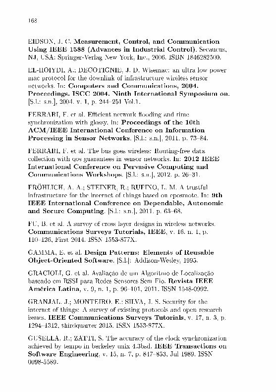
168

EIDSON, J. C. Measurement, Control, and CommunicationUsing IEEE 1588 (Advances in Industrial Control). Secaucus,NJ, USA: Springer-Verlag New York, Inc., 2006. ISBN 1846282500.

EL-HOIYDI, A.; DECOTIGNIE, J. D. Wisemac: an ultra low powermac protocol for the downlink of infrastructure wireless sensornetworks. In: Computers and Communications, 2004.Proceedings. ISCC 2004. Ninth International Symposium on.[S.l.: s.n.], 2004. v. 1, p. 244�251 Vol.1.

FERRARI, F. et al. E�cient network �ooding and timesynchronization with glossy. In: Proceedings of the 10thACM/IEEE International Conference on InformationProcessing in Sensor Networks. [S.l.: s.n.], 2011. p. 73�84.

FERRARI, F. et al. The bus goes wireless: Routing-free datacollection with qos guarantees in sensor networks. In: 2012 IEEEInternational Conference on Pervasive Computing andCommunications Workshops. [S.l.: s.n.], 2012. p. 26�31.

FRÖHLICH, A. A.; STEINER, R.; RUFINO, L. M. A trustfulinfrastructure for the internet of things based on eposmote. In: 9thIEEE International Conference on Dependable, Autonomicand Secure Computing. [S.l.: s.n.], 2011. p. 63�68.

FU, B. et al. A survey of cross-layer designs in wireless networks.Communications Surveys Tutorials, IEEE, v. 16, n. 1, p.110�126, First 2014. ISSN 1553-877X.

GAMMA, E. et al. Design Patterns: Elements of ReusableObject-Oriented Software. [S.l.]: Addison-Wesley, 1995.

GRACIOLI, G. et al. Avaliação de um Algoritmo de Localizaçãobaseado em RSSI para Redes Sensores Sem Fio. Revista IEEEAmérica Latina, v. 9, n. 1, p. 96�101, 2011. ISSN 1548-0992.

GRANJAL, J.; MONTEIRO, E.; SILVA, J. S. Security for theinternet of things: A survey of existing protocols and open researchissues. IEEE Communications Surveys Tutorials, v. 17, n. 3, p.1294�1312, thirdquarter 2015. ISSN 1553-877X.

GUSELLA, R.; ZATTI, S. The accuracy of the clock synchronizationachieved by tempo in berkeley unix 4.3bsd. IEEE Transactions onSoftware Engineering, v. 15, n. 7, p. 847�853, Jul 1989. ISSN0098-5589.

169

HUANG, P. et al. The evolution of mac protocols in wireless sensornetworks: A survey. IEEE Communications Surveys Tutorials,v. 15, n. 1, p. 101�120, First 2013. ISSN 1553-877X.

HUANG, Q. et al. Fast authenticated key establishment protocols forself-organizing sensor networks. In: 2nd ACM WSNA. New York,NY, USA: ACM, 2003. (WSNA '03), p. 141�150. ISBN 1-58113-764-8.

HULBERT, A. et al. An experimental study of big spatial datasystems. In: IEEE International Conference on Big Data (BigData). [S.l.: s.n.], 2016. p. 2664�2671.

IEEE. Ieee standard for a precision clock synchronization protocol fornetworked measurement and control systems. IEEE Std 1588-2008(Revision of IEEE Std 1588-2002), p. c1�269, July 2008.

IEEE Standard for Local and metropolitan area networks�Part 15.4:Low-Rate Wireless Personal Area Networks (LR-WPANs). IEEE Std802.15.4-2011 (Revision of IEEE Std 802.15.4-2006), p. 1�314,Sept 2011.

INSTRUMENTATION, I.; SOCIETY", M. "1451.0 - IEEEStandard for a Smart Transducer Interface for Sensors andActuators�Common Functions, Communication Protocols,and Transducer Electronic Data Sheet (TEDS) Formats".2007. Online. Available at:<http://web.mit.edu/goretkin/Public/ieee1451/4338161.pdf>.

KARLOF, C.; SASTRY, N.; WAGNER, D. Tinysec: a link layersecurity architecture for wireless sensor networks. In: 2nd SenSys.New York, NY, USA: ACM, 2004. p. 162�175. ISBN 1-58113-879-2.Available at: <http://doi.acm.org/10.1145/1031495.1031515>.

LAB, S. I. EPOS - Embedded Parallel Operating System.2017. Available at: <https://epos.lisha.ufsc.br/>.

LEVIS, P. et al. Trickle: A self-regulating algorithm for codepropagation and maintenance in wireless sensor networks. In:Proceedings of the 1st Conference on Symposium onNetworked Systems Design and Implementation - Volume 1.Berkeley, CA, USA: USENIX Association, 2004. (NSDI'04), p. 2�2.Available at: <http://dl.acm.org/citation.cfm?id=1251175.1251177>.

LEWIS, L. L. An introduction to frequency standards. Proceedingsof the IEEE, v. 79, n. 7, p. 927�935, Jul 1991. ISSN 0018-9219.

http://web.mit.edu/goretkin/Public/ieee1451/4338161.pdf

http://doi.acm.org/10.1145/1031495.1031515

http://dl.acm.org/citation.cfm?id=1251175.1251177

170

LISHA. Internet of Things at UFSC. 2017. Available at:<https://iot.ufsc.br/>.

LIU, S.; FAN, K. W.; SINHA, P. Cmac: An energy e�cient mac layerprotocol using convergent packet forwarding for wireless sensornetworks. In: 2007 4th Annual IEEE Communications SocietyConference on Sensor, Mesh and Ad Hoc Communicationsand Networks. [S.l.: s.n.], 2007. p. 11�20. ISSN 2155-5486.

LONARE, S.; WAHANE, G. A survey on energy e�cient routingprotocols in wireless sensor network. In: 2013 FourthInternational Conference on Computing, Communicationsand Networking Technologies (ICCCNT). IEEE, 2013. Availableat: <https://doi.org/10.1109\%2Ficccnt.2013.6726591>.

LU, G.; KRISHNAMACHARI, B.; RAGHAVENDRA, C. S. Anadaptive energy-e�cient and low-latency mac for data gathering inwireless sensor networks. In: Parallel and Distributed ProcessingSymposium, 2004. Proceedings. 18th International. [S.l.: s.n.],2004. p. 224�.

LUK, M. et al. Minisec: A secure sensor network communicationarchitecture. In: 6th IPSN. [S.l.: s.n.], 2007. p. 479 �488.

MARóTI, M. et al. The �ooding time synchronization protocol. In:Proceedings of the 2Nd International Conference onEmbedded Networked Sensor Systems. New York, NY, USA:ACM, 2004. (SenSys '04), p. 39�49. ISBN 1-58113-879-2. Available at:<http://doi.acm.org/10.1145/1031495.1031501>.

MEHTA, A. M.; PISTER, K. S. J. Frequency o�set compensation forcrystal-free 802.15.4 communication. In: International Conferenceon Advanced Technologies for Communications (ATC). [S.l.:s.n.], 2011. p. 45�47. ISSN 2162-1020.

MENDES, L. D.; RODRIGUES, J. J. A survey on cross-layersolutions for wireless sensor networks. Journal of Network andComputer Applications, v. 34, n. 2, p. 523 � 534, 2011. ISSN1084-8045. E�cient and Robust Security and Services of WirelessMesh Networks.

MILLS, D. Internet time synchronization: the network time protocol.IEEE Transactions on Communications, v. 39, n. 10, p.1482�1493, Oct 1991. ISSN 0090-6778.

http://doi.acm.org/10.1145/1031495.1031501

171

NIAN, M. G. lesta SIVA, J.; POELLABAUER, C. Radiofrequency-based indoor localization in ad-hoc networks. In: ORTIZ, J.(Ed.). Ad Hoc Networks. InTech, 2017. cap. 6. Available at:<https://www.intechopen.com/books/ad-hoc-networks/radio-frequency-based-indoor-localization-in-ad-hoc-networks>.

OKAZAKI, A. M.; FRÖHLICH, A. A. ADHOP: an Energy AwareRouting Algorithm for Mobile Wireless Sensor Networks. In: IEEESENSORS. Taipei, Taiwan: [s.n.], 2012. Available at:<http://www.lisha.ufsc.br/pub/Okazaki\ Sensors\ 2012.pdf>.

OLIVEIRA, P. et al. Sincronização de Tempo a nível de SO utilizandoo protocolo IEEE1588. In: Brazilian Symposium on ComputingSystems Engineering. Natal, Brazil: [s.n.], 2012. ISBN978-0-7695-4929-3. Available at: <http://sbesc.lisha.ufsc.br-/sbesc2012/tiki-download\ �le.php?�leId=115>.

OPENSIM. OMNeT++ - Objective Modular NetworkTestbed in C++. 2017. Available at: <https://omnetpp.org/>.

PATIL, M.; BIRADAR, R. C. A survey on routing protocols inwireless sensor networks. In: IEEE. Networks (ICON), 2012 18thIEEE International Conference on. [S.l.], 2012. p. 86�91.

PIRES, R. P.; WANNER, L. F.; FRÖHLICH, A. A. An E�cientCalibration Method for RSSI-based Location Algorithms. In: 6thInternational IEEE Conference on Industrial Informatics.Daejeon, Korea: [s.n.], 2008. p. 1183�1188. ISBN 978-1-4244-2170-1.

POLASTRE, J.; HILL, J.; CULLER, D. Versatile low power mediaaccess for wireless sensor networks. In: ACM SenSys. New York,USA: [s.n.], 2004. p. 95�107. ISBN 1-58113-879-2.

REGHELIN, R.; FRÖHLICH, A. A. A Decentralized LocationSystem for Sensor Networks Using Cooperative Calibration andHeuristics. In: 9th ACM/IEEE International Symposium onModeling, Analysis and Simulation of Wireless and MobileSystems. Torremolinos, Malaga, Spain.: [s.n.], 2006. p. 139�146.ISBN 1-59593-477-4.

RESNER, D. Estabelecimento de Chaves e ComunicaçãoSegura para a Internet das Coisas. Florianópolis: [s.n.], 2014.67 p. B.Sc. Thesis. Available at:<http://www.lisha.ufsc.br/pub/Resner\ BSC\ 2014.pdf>.

http://www.lisha.ufsc.br/pub/Okazaki_Sensors_2012.pdf

http://sbesc.lisha.ufsc.br/sbesc2012/tiki-download_file.php?fileId=115

http://sbesc.lisha.ufsc.br/sbesc2012/tiki-download_file.php?fileId=115

http://www.lisha.ufsc.br/pub/Resner_BSC_2014.pdf

172

RESNER, D.; ARAUJO, G. M. de; FRÖHLICH, A. A. On theImpact of Dynamic Routing Metrics on a Geographic Protocol forWSNs. In: Brazilian Symposium on Computing SystemsEngineering. João Pessoa, Brazil: [s.n.], 2016. Available at:<http://www.lisha.ufsc.br/pub/Resner\ SBESC\ 2016.pdf>.

RESNER, D.; ARAUJO, G. M. de; FRÖHLICH, A. A. Design andImplementation of a Cross-Layer IoT Protocol. Science ofComputer Programming, v. 0, n. 0, p. 0, 2017. ISSN 0000-0000.

RESNER, D.; FRÖHLICH, A. A. Design Rationale of a Cross-layer,Trustful Space-Time Protocol for Wireless Sensor Networks. In: 20thIEEE International Conference on Emerging Technologiesand Factory Automation (ETFA). Luxembourg, Luxembourg:[s.n.], 2015. p. 1�8. Available at:<http://www.lisha.ufsc.br/pub/Resner\ ETFA\ 2015.pdf>.

RESNER, D.; FRÖHLICH, A. A. Key Establishment and TrustfulCommunication for the Internet of Things. In: 4th InternationalConference on Sensor Networks (SENSORNETS 2015).Angers, France: [s.n.], 2015. p. 197�206. ISBN 978-989-758-086-4.Available at:<http://www.lisha.ufsc.br/pub/Resner\ SENSORNETS\ 2015.pdf>.

RESNER, D.; FRÖHLICH, A. A. TSTP MAC: A Foundation for theTrustful Space-Time Protocol. In: 14th IEEE/IFIP InternationalConference on Embedded and Ubiquitous Computing(EUC). Paris, France: [s.n.], 2016.

RESNER, D.; FRÖHLICH, A. A.; WANNER, L. F. SpeculativePrecision Time Protocol: submicrosecond clock synchronization forthe IoT. In: 21th IEEE International Conference on EmergingTechnologies and Factory Automation (ETFA). Berlin,Germany: [s.n.], 2016.

SANTOS, T. R. dos; FRÖHLICH, A. A. A Customizable Componentfor Low-Level Communication Software. In: 19th AnnualSymposium on High Performance Computing Systems andApplications. Guelph, Canada: [s.n.], 2005. p. 58�64. ISBN0-7695-2343-9.

SCHMID, T.; DUTTA, P.; SRIVASTAVA, M. B. High-resolution,low-power time synchronization an oxymoron no more. In:Proceedings of the 9th ACM/IEEE International Conference

http://www.lisha.ufsc.br/pub/Resner_SBESC_2016.pdf

http://www.lisha.ufsc.br/pub/Resner_ETFA_2015.pdf

http://www.lisha.ufsc.br/pub/Resner_SENSORNETS_2015.pdf

173

on Information Processing in Sensor Networks. New York, NY,USA: ACM, 2010. (IPSN '10), p. 151�161. ISBN 978-1-60558-988-6.Available at: <http://doi.acm.org/10.1145/1791212.1791231>.

STEINER, R. V. et al. Performance Evaluation of Receiver BasedMAC Using Con�gurable Framework in WSNs. In: IEEE WirelessCommunications and Networking Conference (WCNC).Shanghai, China: [s.n.], 2013. p. 884�889. ISBN 978-1-4673-5939-9.Available at:<http://www.lisha.ufsc.br/pub/Steiner\ WCNC\ 2013.pdf>.

SUO, H. et al. Security in the internet of things: A review. In:ICCSEE. [S.l.: s.n.], 2012. v. 3, p. 648�651.

TEXAS INSTRUMENTS. CC2538 Powerful WirelessMicrocontroller System-On-Chip for 2.4-GHz IEEE 802.15.4,6LoWPAN, and ZigBee Applications datasheet. [S.l.], 4 2015.Rev. D.

ZHOU, H. et al. Frequency Accuracy and StabilityDependencies of Crystal Oscillators. [S.l.], 11 2008.

http://doi.acm.org/10.1145/1791212.1791231

http://www.lisha.ufsc.br/pub/Steiner_WCNC_2013.pdf

Appendix A -- Additional simulation results

177

0 100 200 300 400 500 600

0.40

0.45

0.50

0.55

0.60

0.65


Mea

n la

tenc

y (s

)

●

●

●

●

● ●●

●

●

●

SpeculativeExplicit


500 1000 1500

0.37

0.38

0.39

0.40

0.41

0.42


Mea

n la

tenc

y (s

)

●

●

●

●

●

●

●

SpeculativeExplicit


Figure 96: Average latency for environment monitoring scenario,d=300s.

The simulation results in this Appendix are similar to the onespresented and discussed in Chapter 4, and are included for completion.

A.1 SYNCHRONIZATION

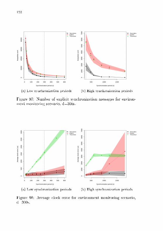
178

0 100 200 300 400 500 600

020

000

4000

060

000

8000

0


Kee

paliv

es s

ent

●

●

●

●

●●

●● ●

●



500 1000 15000

1000

2000

3000

4000

5000

6000

7000


Kee

paliv

es s

ent

●

●

●

●

●

●

●



Figure 97: Number of explicit synchronization messages for environ-ment monitoring scenario, d=300s.

0 100 200 300 400 500 600

050

010

0015

0020

0025

0030

00


Ave

rage

clo

ck e

rror

(us

)

● ● ● ●● ● ●

●●

●



500 1000 1500

010

0020

0030

0040

0050

0060

0070

00


Ave

rage

clo

ck e

rror

(us

)

●● ●

●

●

●

●




179

0 100 200 300 400 500 600

0e+

001e

+05

2e+

053e

+05


The

oret

ical

ene

rgy

gain

(J)

●

●

●

●● ● ● ● ●

●

SpeculativeExplicit


500 1000 1500

−50

000

5000

1000

015

000

2000

025

000


The

oret

ical

ene

rgy

gain

(J)

●

●

● ●●

●

●

SpeculativeExplicit



0 100 200 300 400 500 600

6080

100

120


Est

imat

ed n

etw

ork

lifet

ime

(day

s)

●

●

●

●

●

●

●

●

●

●

SpeculativeExplicit


500 1000 1500

120

125

130

135


Est

imat

ed n

etw

ork

lifet

ime

(day

s)

●

●

●

●●

●

●

SpeculativeExplicit


Figure 100: Estimated network lifetime for environment monitoringscenario, d=300s.

180

0 500 1000 1500

0.6

0.7

0.8

0.9

1.0

1.1


Mea

n la

tenc

y (s

)

●

●

●

●

●●

●● ● ● ● ●

●

SpeculativeExplicit


1000 1500 2000 2500 3000 35000.

540.

550.

560.

570.

580.

590.

60


Mea

n la

tenc

y (s

)

●

●

●●

●

●

●

SpeculativeExplicit


Figure 101: Average latency for environment monitoring scenario,d=900s.

0 500 1000 1500

020

000

4000

060

000

8000

0


Kee

paliv

es s

ent

●

●

●

●

●●

●●

● ● ● ●

●



1000 1500 2000 2500 3000 3500

050

010

0015

0020

0025

00


Kee

paliv

es s

ent

●

●

●

● ●

●

●



Figure 102: Number of explicit synchronization messages for environ-ment monitoring scenario, d=900s.

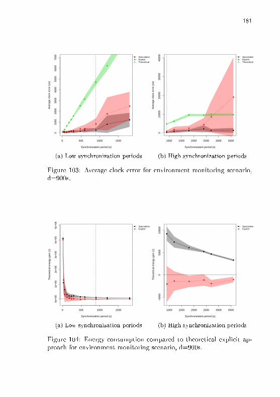
181

0 500 1000 1500

010

0020

0030

0040

0050

0060

0070

00


Ave

rage

clo

ck e

rror

(us

)

●●● ● ● ● ●● ●

●

●

●

●



1000 1500 2000 2500 3000 3500

010

000

2000

030

000

4000

0


Ave

rage

clo

ck e

rror

(us

)

●●

●

●

●

●

●




0 500 1000 1500

0e+

001e

+05

2e+

053e

+05

4e+

055e

+05


The

oret

ical

ene

rgy

gain

(J)

●

●

●

●● ● ● ● ● ● ● ●

●

SpeculativeExplicit


1000 1500 2000 2500 3000 3500

−50

000

5000

1000

0


The

oret

ical

ene

rgy

gain

(J)

●

● ●●

●

●

●

SpeculativeExplicit



182

0 500 1000 1500

5010

015

020

025

0


Est

imat

ed n

etw

ork

lifet

ime

(day

s)

●

●

●

●

●

●

●

●

●

●

●

●

●

SpeculativeExplicit


1000 1500 2000 2500 3000 3500

230

240

250

260

270


Est

imat

ed n

etw

ork

lifet

ime

(day

s)

●

●

●

●

●

●

●

SpeculativeExplicit


Figure 105: Estimated network lifetime for environment monitoringscenario, d=900s.

183


Zero

Expiry Distance

Effort Distance

Random

Distance


0 10 20 30 40


Expiry Distance


Zero

Effort Distance

Random

Distance

Mean latency (s)

0.00 0.01 0.02 0.03 0.04 0.05

(b) Mean latency

Figure 106: Estimated network lifetime and mean latency for LISHAo�ce scenario under di�erent routing metrics.

A.2 ROUTING METRICS

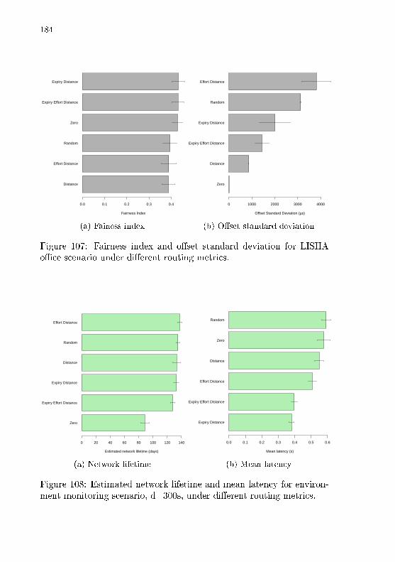
184

Distance

Effort Distance

Random

Zero


Expiry Distance

Fairness Index

0.0 0.1 0.2 0.3 0.4

(a) Fainess index

Zero

Distance


Expiry Distance

Random

Effort Distance


0 1000 2000 3000 4000


Figure 107: Fairness index and o�set standard deviation for LISHAo�ce scenario under di�erent routing metrics.

Zero


Expiry Distance

Distance

Random

Effort Distance


0 20 40 60 80 100 120 140


Expiry Distance


Effort Distance

Distance

Zero

Random

Mean latency (s)

0.0 0.1 0.2 0.3 0.4 0.5 0.6

(b) Mean latency


185

Expiry Distance

Distance

Zero

Random


Effort Distance

Fairness Index

0.0 0.1 0.2 0.3 0.4 0.5 0.6 0.7

(a) Fainess index

Zero


Expiry Distance

Effort Distance

Distance

Random


0 5000 10000 15000 20000 25000 30000


Figure 109: Fairness index and o�set standard deviation for environ-ment monitoring scenario, d=300s, under di�erent routing metrics.

Zero

Expiry Distance


Random

Distance

Effort Distance


0 50 100 150 200 250



Expiry Distance

Effort Distance

Distance

Zero

Random

Mean latency (s)

0.0 0.2 0.4 0.6 0.8

(b) Mean latency


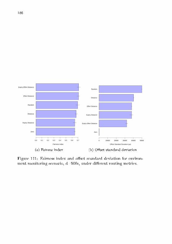
186

Zero

Expiry Distance

Distance

Random

Effort Distance


Fairness Index

0.0 0.1 0.2 0.3 0.4 0.5 0.6 0.7

(a) Fainess index

Zero


Expiry Distance

Effort Distance

Distance

Random


0 10000 20000 30000 40000 50000


Figure 111: Fairness index and o�set standard deviation for environ-ment monitoring scenario, d=900s, under di�erent routing metrics.

Appendix B -- Scienti�c Publications

189

The following articles were direct products of the work presentedin this dissertation, published in scienti�c journals or conference pro-ceedings:

1.RESNER, D.; FROHLICH, A. A. . Key Establishment andTrustful Communication for the Internet of Things. In:4th International Conference on Sensor Networks (SENSORNETS),2015, ESEO. p. 197-206.

2.RESNER, D.; FROHLICH, A. A. . Design rationale of across-layer, Trustful Space-Time Protocol for WirelessSensor Networks. In: 2015 IEEE 20th Conference on EmergingTechnologies & Factory Automation (ETFA), 2015, Luxembourg.

3.RESNER, D.; FROHLICH, A. A. . TSTP MAC: a Cross-Layer, Geographic, Receiver-Based MAC Protocol forWSNs. In: Brazilian Symposium on Computing Systems Engi-neering (SBESC), 2015, Foz do Iguaçu.

4.RESNER, D.; FROHLICH, A. A. . TSTP MAC: A Founda-tion for the Trustful Space-Time Protocol. In: 2016 IEEEIntl Conference on Embedded and Ubiquitous Computing (EUC),Paris. 2016, p. 40.

5.RESNER, D.; FROHLICH, A. A.; WANNER, L. F. . Spec-ulative Precision Time Protocol: Submicrosecond clocksynchronization for the IoT. In: 2016 IEEE 21st InternationalConference on Emerging Technologies and Factory Automation(ETFA), 2016, Berlin. 2016.

6.RESNER, D.; ARAUJO, G. M. ; FROHLICH, A. A. . On theImpact of Dynamic Routing Metrics on a GeographicProtocol for WSNs. In: 2016 VI Brazilian Symposium onComputing Systems Engineering (SBESC), 2016, João Pessoa.p. 109.

7.SILVA, D. S. ; RESNER, D. ; SOUZA, R. L. ; MARTINA, J. E.. Formal Veri�cation of a Cross-Layer, Trustful Space-Time Protocol for Wireless Sensor Networks. In: LectureNotes in Computer Science. 0ed.: Springer International Pub-lishing, 2016, v. , p. 426-443.

8.SUSIN, M. M. ; WANNER, L. F. ; RESNER, D. ; FROHLICH,A. A. . Time Synchronization under Temperature and

190

Distance Variations. In: 2017 VII Brazilian Symposium onComputing Systems Engineering (SBESC), 2017, Curitiba. p.167.

9.RESNER, D.; ARAUJO, G. M. ; FRÖHLICH, A. A. . Designand Implementation of a Cross-Layer IoT Protocol. In:Science Of Computer Programming, 2017.

Universidade ederalF de Santa Catarina Biblioteca ... · for the Embedded Parallel Operating System...

Documents

Transcript of Universidade ederalF de Santa Catarina Biblioteca ... · for the Embedded Parallel Operating System...