UNIVERSIDADE TECNOLÓGICA FEDERAL DO PARANÁ

PROGRAMA DE PÓS-GRADUAÇÃO EM ENGENHARIA ELÉTRICA

DIERLI MAIARA DA ROSA MASCHIO

UMA ABORDAGEM ORIENTADA A EVENTOS PARA O

PLANEJAMENTO DE RECURSOS EM SISTEMAS DE GERAÇÃO

DISTRIBUÍDA DE ENERGIA

DISSERTAÇÃO

PATO BRANCO

2021

DIERLI MAIARA DA ROSA MASCHIO

UMA ABORDAGEM ORIENTADA A EVENTOS PARA O

PLANEJAMENTO DE RECURSOS EM SISTEMAS DE GERAÇÃO

DISTRIBUÍDA DE ENERGIA

An Event-Driven Approach For Resources Planning In Distributed Power

Generation Systems

Dissertação apresentado(a) como requisito par-cial à obtenção do título de Mestra em Engen-haria Elétrica, do Programa de Pós-Graduaçãoem Engenharia Elétrica, da Universidade Tec-nológica Federal do Paraná.

Orientador: Prof. Dr. Marcelo TeixeiraCoorientador: Prof. Dr. Jean Patric da Costa

PATO BRANCO

2021

4.0 Internacional

Esta licença permite o download e o compartilhamento da obradesde que sejam atribuídos créditos ao(s) autor(es), sem a possibil-idade de alterá-la ou utilizá-la para fins comerciais.

Ministério da Educação Universidade Tecnológica Federal do Paraná

Campus Pato Branco

DIERLI MAIARA DA ROSA MASCHIO

UMA ABORDAGEM ORIENTADA A EVENTOS PARA O PLANEJAMENTO DE RECURSOS EM SISTEMAS DE GERAÇÃO DISTRIBUÍDA DE ENERGIA

Trabalho de pesquisa de mestrado apresentado como requisito para obtenção do título de Mestra Em EngenhariaElétrica da Universidade Tecnológica Federal do Paraná (UTFPR). Área de concentração: Sistemas E ProcessamentoDe Energia.

Data de aprovação: 14 de Junho de 2021

Prof Marcelo Teixeira, Doutorado - Universidade Tecnológica Federal do Paraná

Prof Andre Eugenio Lazzaretti, - Universidade Tecnológica Federal do Paraná

Prof Dieky Adzkiya, Doutorado - Sepuluh Nopember Institute Of Technology

Prof Jean Marc Stephane Lafay, - Universidade Tecnológica Federal do Paraná

Documento gerado pelo Sistema Acadêmico da UTFPR a partir dos dados da Ata de Defesa em 14/06/2021.

À minha família e ao meu amor Rodrigo.

ACKNOWLEDGEMENTS

Este trabalho não poderia ser terminado sem a ajuda de diversas pessoas e/ou institu-

ições às quais presto minha homenagem. Certamente esses parágrafos não irão atender a todas

as pessoas que fizeram parte dessa importante fase de minha vida. Portanto, peço desculpas

àquelas que não estão presentes entre estas palavras, mas elas podem estar certas que fazem

parte do meu pensamento e de minha gratidão.

A minha família, meu pai Vanilso, minha mãe Roseli, minha irmã Diulia, pelo carinho

e incentivo, vocês são meus exemplos de vida.

Ao meu eterno namorado Rodrigo, pelo carinho, paciência, respeito e total apoio em

minhas decisões.

A todas as amigas, em especial a Daiane e Carol pela amizade, e por estarem sempre

presentes em todos os momentos da minha trajetória acadêmica e pessoal.

Aos meus orientadores, que mostraram os caminhos a serem seguidos, em especial

ao professor Marcelo Teixeira que acreditou em meu potencial e não mediu esforços para me

ajudar a realizar e concluir este trabalho.

A todos os professores do departamento, da banca avaliadora, e demais que ajudaram

de forma direta e indireta na conclusão deste trabalho.

O cientista não é o homem que fornece as

verdadeiras respostas; é quem faz as

verdadeiras perguntas. (Claude Lévi-Strauss)

ABSTRACT

MASCHIO, Dierli Maiara da Rosa. An Event-Driven Approach For Resources Planning InDistributed Power Generation Systems. 2021. 47 p. Dissertation (Master’s Degree inElectrical Engineering) – Universidade Tecnológica Federal do Paraná. Pato Branco, 2021.

Renewable power generation systems stand as astraightforward alternative to complement theenergy grid of the future. Physically, generation components have distributed nature and theywork individually to supply centralised microgrids, which interface them with the main powergrid and consumers. As microgrid components are non-cooperative entities, engineers are lim-ited to plan resources consumption, fulfil unit commitments, stratify time, cost, environmentalimpact, quality of energy, etc. In this paper, we exploit the event-driven behaviour of microgridsto provide ways for them to recognise, communicate, and cooperate with each other towardscommon goals. We first design microgrids and generators as self-controlled cyber-physicalagents that communicate with each other and with the main power grid. Then, we develop aPetri net simulation model that estimates customisation policies to be applied backover the mi-crogrid via event-based control. Results show that in some cases it is possible to save effort (andresources) of power generation by replacing reactiveness for a more balanced, context-aware,energy chain. A real photovoltaic plant is modelled by our approach with 86% accuracy.

Keywords: Microgrids. Modelling. Simulation. Control. Cooperative power generation.

RESUMO

MASCHIO, Dierli Maiara da Rosa. Uma Abordagem Orientada a Eventos para oPlanejamento de Recursos em Sistemas de Geração Distribuída de Energia. 2021. 47 f.Dissertação (Mestrado em Engenharia Elétrica) – Universidade Tecnológica Federal do Paraná.Pato Branco, 2021.

Os sistemas de geração de energia renovável são uma alternativa direta para complementara rede de energia do futuro. Fisicamente, os componentes de uma microrrede têm naturezadistribuída e funcionam individualmente para alimentar microrredes centralizadas, que tratamda interação com a rede elétrica principal e os consumidores. Como os componentes de umamicrorrede são entidades não cooperativas, a engenharia enfrenta limitações para planejar oconsumo de recursos, o cumprimento de contratos, estratificar tempo, custo, impacto ambien-tal, qualidade de energia, etc. Nesta dissertação, uma microrrede é explorada em relação aoseu comportamento orientado a eventos, visando o processamento desses eventos com foco noplanejamento de recursos de geração. A ideia é que os componentes da microrrede reconheçamseu contexto, se comuniquem e cooperem entre si em prol de objetivos comuns. Inicialmente,microrredes e geradores são projetados como agentes ciberfísicos que se autocontrolam e secomunicam entre si e com a rede elétrica principal. Em seguida, propõe-se um modelo de sim-ulação em redes de Petri que estima políticas de personalização para serem aplicadas sobre amicrorrede, por meio de um nível de controle baseado em eventos discretos. Os resultados sug-erem a possibilidade de economizar esforço e recursos de geração de energia substituindo-sea reatividade da decisão de controle por uma decisão mais equilibrada, que reconhece e pon-dera aspectos de toda a cadeia de energia. Uma planta fotovoltaica real é modelada por nossaabordagem com precisão de 86%.

Palavras-chave: Microrredes. Modelagem. Simulação. Controle. Geração de energia coopera-tiva.

LIST OF FIGURES

Figure 1 – State-of-art summary and the directions taken in this paper. . . . . . . . . . 13Figure 2 – The Basic architecture of a microgrid. . . . . . . . . . . . . . . . . . . . . 15Figure 3 – Small manufacturing system example. . . . . . . . . . . . . . . . . . . . . 17Figure 4 – Example of a DES model, where G = X Y . . . . . . . . . . . . . . . . . 18Figure 5 – Example of DES control, for K = E G. . . . . . . . . . . . . . . . . . . 18Figure 6 – Workflow models for the manufacturing system in Fig. 3. . . . . . . . . . . 20Figure 7 – Layout of the proposed framework for distributed power generation. . . . . 22Figure 8 – Plant model Multiple-level power generator. . . . . . . . . . . . . . . . . . 23Figure 9 – Specifications multiple-level power generator. . . . . . . . . . . . . . . . . 23Figure 10 – Plant and specification of a single-level generator. . . . . . . . . . . . . . . 24Figure 11 – Plant model of a microgrid. . . . . . . . . . . . . . . . . . . . . . . . . . . 25Figure 12 – A basic GSPN model for a power generator. . . . . . . . . . . . . . . . . . 27Figure 13 – Performance evaluation of a photovoltaic panel under variable resources. . . 30Figure 14 – Partial layout of the real photovoltaic system at UTFPR. . . . . . . . . . . . 32Figure 15 – Estimated versus measured power generations . . . . . . . . . . . . . . . . 34Figure 16 – Proposed GSPN to design plug-and-play microgrid components. . . . . . . 35Figure 17 – GSPN model for the case study. . . . . . . . . . . . . . . . . . . . . . . . 37Figure 18 – Storage dimensioning (#RB) under three load profiles (#RL): 50 to 150

tokens – 17000W to 53040W , with λB = 1s. . . . . . . . . . . . . . . . . . 39Figure 19 – Storage dimensioning (#RB) under three load profiles (#RL): 50 to 150

tokens – 17000W to 53040W , with λB = 0.1s. . . . . . . . . . . . . . . . . 40

LIST OF TABLES

Table 1 – Input parameters derivation for λ2. . . . . . . . . . . . . . . . . . . . . . . . 28Table 2 – Plant potential and distribution. . . . . . . . . . . . . . . . . . . . . . . . . 33Table 3 – Input parameters of the model. . . . . . . . . . . . . . . . . . . . . . . . . . 33Table 4 – Arc conditions for the microgrid model. . . . . . . . . . . . . . . . . . . . . 36

CONTENTS

1 INTRODUCTION . . . . . . . . . . . . . . . . . . . . . . . . . . . . . . 11

2 LITERATURE OVERVIEW . . . . . . . . . . . . . . . . . . . . . . . . 13

3 BACKGROUND . . . . . . . . . . . . . . . . . . . . . . . . . . . . . . . 153.1 THE DISCRETE NATURE OF SYSTEMS . . . . . . . . . . . . . . . . 163.2 DISCRETE EVENT SYSTEMS . . . . . . . . . . . . . . . . . . . . . . 173.3 PETRI NETS . . . . . . . . . . . . . . . . . . . . . . . . . . . . . . . . . 19

4 PROPOSED WORKFLOW . . . . . . . . . . . . . . . . . . . . . . . . . 224.1 MODELLING AND CONTROL . . . . . . . . . . . . . . . . . . . . . . 234.1.1 Multiple-level generation modelling . . . . . . . . . . . . . . . . . . . . . . 234.1.2 Single-level generation modelling . . . . . . . . . . . . . . . . . . . . . . . 244.2 MICROGRID MODELLING . . . . . . . . . . . . . . . . . . . . . . . . 244.3 CONTROL SYNTHESIS . . . . . . . . . . . . . . . . . . . . . . . . . . 25

5 PETRI NET-BASED CUSTOMISATION . . . . . . . . . . . . . . . . . 275.1 A CASE STUDY ON PHOTOVOLTAIC GENERATION . . . . . . . . 285.1.1 Photovoltaic simulation and analysis . . . . . . . . . . . . . . . . . . . . . 29

6 CASE STUDY INVOLVING A REAL POWER PLANT . . . . . . . . . 326.1 REAL SYSTEM SETUP . . . . . . . . . . . . . . . . . . . . . . . . . . 326.1.1 Model simulation and analysis . . . . . . . . . . . . . . . . . . . . . . . . . 336.2 MICROGRID MODELLING . . . . . . . . . . . . . . . . . . . . . . . . 346.2.1 Input parameters for M . . . . . . . . . . . . . . . . . . . . . . . . . . . . 356.2.2 Microgrid simulations and analysis . . . . . . . . . . . . . . . . . . . . . . 376.3 EXAMPLE OF COOPERATIVE DISTRIBUTION . . . . . . . . . . . 40

7 CONCLUSIONS AND PERSPECTIVES . . . . . . . . . . . . . . . . . 42

REFERENCES . . . . . . . . . . . . . . . . . . . . . . . . . . . . . . . . 43

11

1 INTRODUCTION

In the current model of power generation systems, a substantial amount of electricity

still depends on non-renewable high-carbon sources (IEA, 2018). In recent years, however, re-

newable sources have appeared as an effective low-carbon way to supply the energy grid of

the future (NEHRIR et al., 2011). Photovoltaic (PV), wind, and small hydroelectric plants,

for example, have shown to be sustainable alternatives. Physically, they are autonomous and

distributed entities that work together to supply centralised infrastructures called microgrids,

which also manage the interaction with the external main power grid (MPG) and consumers.

(HATZIARGYRIOU et al., 2007; LASSETER; PIAGI, 2004).

A microgrid coordinates generation, consumption, and storage, working either con-

nected (on-grid) or not (off-grid) to the MPG (ASMUS, 2010; FARHANGI; JOOS, 2019). It

is also expected to regulate its interaction with other components, protecting them from distur-

bances caused by its intermittent sources (MIRSAEIDI et al., 2014; HARITZA et al., 2016;

DJELLOULI et al., 2019; ZOKA et al., 2004). Therefore, an important matter in microgrids

is to be able to anticipate possible fluctuations that may disturb the energy supplying (JANA;

CHAKRABORTY, 2020; OLIVARES et al., 2014). This can be revealed, for example, by mon-

itoring the real system. However, this option fails to provide in-advance information that could

benefit planning, contingency, and predictive corrections. These steps are more impacted by

modelling approaches that anticipate metrics of interest without necessarily depending on on-

line systems (PAULISTA et al., 2019; SIMON et al., 2021).

In the literature, some modelling approaches have focused on the continuous be-

haviour of microgrids (PARVANIA; SCAGLIONE, 2015; JANA; CHAKRABORTY, 2020;

NAVERSEN et al., 2019). However, some events (e.g., sensing, bounds, violations) happen in

a discrete manner and variations (e.g., user profile, consumption, faults) are essentially stochas-

tic, justifying event-based complements to the continuous grid control. Event processing and

simulation have been used in microgrids management (CASSETTARI et al., 2017; JANA;

CHAKRABORTY, 2020; TSAMPASIS et al., 2016), but essentially as support for reactive

actions, so that proactive planning steps are still unclear.

In this paper, event processing is exploited for predictive engineering. We show how

microgrid components can be exposed as Discrete Event Systems (DESs) (CASSANDRAS;

LAFORTUNE, 2008) that are processed both for control and optimisation. Control is handled

12

by using synthesis methods (RAMADGE; WONHAM, 1989) that have Finite State Machines

(FSMs) (CASSANDRAS; LAFORTUNE, 2008) as modelling foundation. For the optimisation

step, a timed Petri Net (KARTSON et al., 1995) simulation model is proposed to discover ways

for microgrid components to interact cooperatively towards common goals. Our approach can

be seen as a software layer that orchestrates discrete events before triggering continuous actions

in the system, taking advantages from the abstraction level in which DESs are designed and

specified, and from the reconfiguration possibilities that emerge from event processing.

A real PV plant is used to illustrate and validate our approach. Initially, a single PV

module is evaluated, which is them generalised for sets of modules. In both cases, the per-

formance of the real plant is compared with estimations anticipated by our model and their

proximity reveals the model’s accuracy. The single-module analysis was also reproduced in

Matlab/Simulink, using single-diode equivalent circuit model, for the sake of comparison, but

the generalisation for the second analysis is not straightforward. Overall, results suggest that our

approach has potential to reduce the level of uncertainties provoked by unstable power sources,

by anticipating their behaviour, which make it feasible to establish cooperation policies in power

generation plants.

In the following, literature and concepts are outlined in Sections 3 and 2; Section 4

introduces the architecture that will be modelled and controlled in Sections 4.1 and 5, tested in

Section 6, and compared in Section 6.3. Conclusions and perspectives are shown in Section 7.

13

2 LITERATURE OVERVIEW

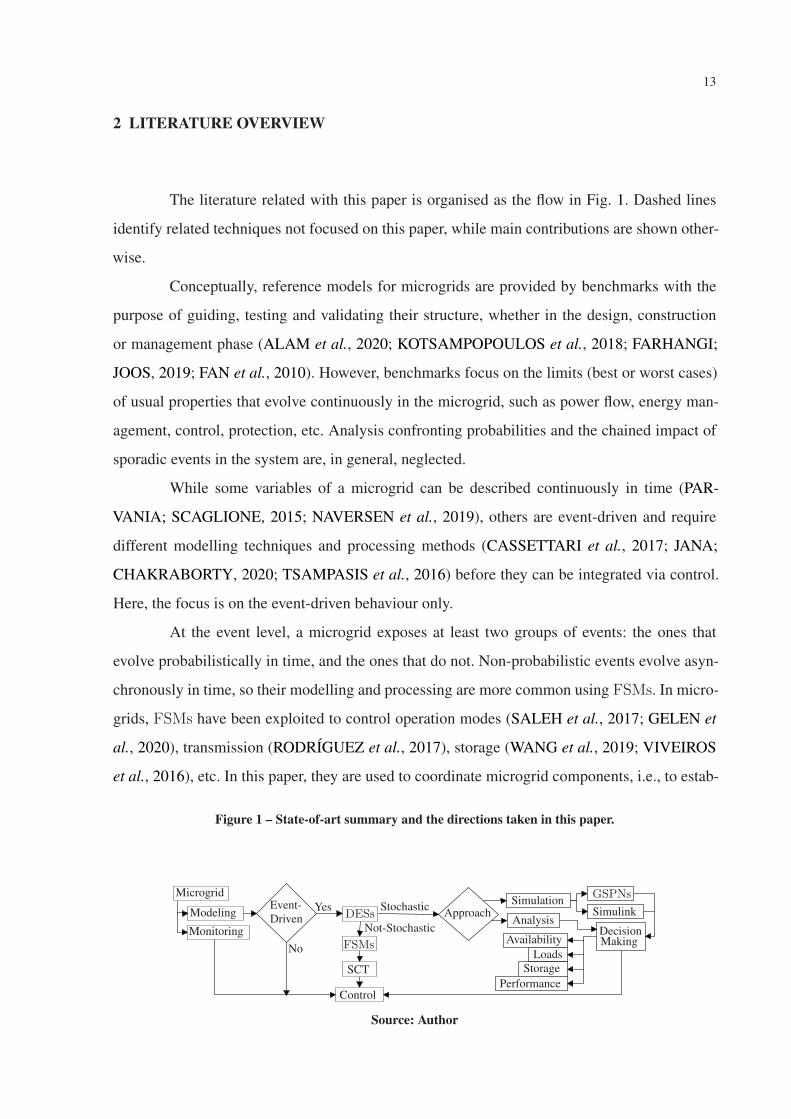
The literature related with this paper is organised as the flow in Fig. 1. Dashed lines

identify related techniques not focused on this paper, while main contributions are shown other-

wise.

Conceptually, reference models for microgrids are provided by benchmarks with the

purpose of guiding, testing and validating their structure, whether in the design, construction

or management phase (ALAM et al., 2020; KOTSAMPOPOULOS et al., 2018; FARHANGI;

JOOS, 2019; FAN et al., 2010). However, benchmarks focus on the limits (best or worst cases)

of usual properties that evolve continuously in the microgrid, such as power flow, energy man-

agement, control, protection, etc. Analysis confronting probabilities and the chained impact of

sporadic events in the system are, in general, neglected.

While some variables of a microgrid can be described continuously in time (PAR-

VANIA; SCAGLIONE, 2015; NAVERSEN et al., 2019), others are event-driven and require

different modelling techniques and processing methods (CASSETTARI et al., 2017; JANA;

CHAKRABORTY, 2020; TSAMPASIS et al., 2016) before they can be integrated via control.

Here, the focus is on the event-driven behaviour only.

At the event level, a microgrid exposes at least two groups of events: the ones that

evolve probabilistically in time, and the ones that do not. Non-probabilistic events evolve asyn-

chronously in time, so their modelling and processing are more common using FSMs. In micro-

grids, FSMs have been exploited to control operation modes (SALEH et al., 2017; GELEN et

al., 2020), transmission (RODRÍGUEZ et al., 2017), storage (WANG et al., 2019; VIVEIROS

et al., 2016), etc. In this paper, they are used to coordinate microgrid components, i.e., to estab-

Figure 1 – State-of-art summary and the directions taken in this paper.

Event-Driven

Microgrid

Monitoring

DESs

FSMs

SCT

Control

ApproachSimulation

AnalysisSimulink

GSPNs

DecisionMaking

LoadsAvailability

StoragePerformance

Yes

No

Not-Stochastic

StochasticModeling

Source: Author

14

lish the way microgrids perceive and interact with low-level components (e.g., generators) and

how it interfaces them with high-level resources (e.g., MPG).

By modelling low-level (sensing, generators, resources), medium level (microgrid ),

and high level (MPG) components as FSMs, it is possible to process control synthesis in order

to make sure that they behave as expected (SALEH et al., 2017; RODRÍGUEZ et al., 2017;

GHASAEI et al., 2020; GELEN et al., 2020). Furthermore, it also becomes possible to choose

certain controlled events in the system and use them as communication channels to trigger smart

decisions that could make components to cooperate towards common goals. This is different

from what the literature has established so far.

In this paper, cooperation policies for microgrids are discovered using simulation mod-

els that exploit the probabilistic nature of events. The modelling of probabilistic events requires

resources other than ordinary FSMs. Usually, probability distributions are associated with the

occurrences of events, so that they can be synchronised in time. One option is to adopt Petri

Nets (MURATA, 1989) and their options for both simulation and state-space analysis.

In microgrids, Petri Nets have been used for properties assessment, such as current

and tension flows (LU et al., 2016; CHAMORRO et al., 2012; SCHOONENBERG; FARID,

2017), for availability estimation (SIMON et al., 2021), and also to discover the capacity of in-

tegrated energy sources (JANA; CHAKRABORTY, 2020). In this paper, an extension of timed

Petri Nets, called GSPN (KARTSON et al., 1995), is adopted to complement the event-driven

control with decision making capabilities. By modelling generation, storage, load, MPG, and

their integrated flow, the proposed GSPN model can anticipate actions to be triggered by the

event-driven controller, so that it results in a more balanced strategy for power generation.

15

3 BACKGROUND

Renewable energy sources can be exploited over the time without depleting the natural

resource in use. This reduces the dependence from fossil fuels and the emissions of gases into

the environment. However, their intermittent nature impacts on the power grid reliability (DEN-

HOLM et al., 2010), as the generation rate fluctuates with the resource availability, affecting

the quality of energy.

One way to obtain a more balanced production is to integrate different, possibly hetero-

geneous, energy sources into the same grid, so that they can complement each other. Microgrid

is the infrastructure that integrates different energy sources and related resources (CATALãO,

2017; LASSETER; PIAGI, 2004), as shown in Fig. 2.

Figure 2 – The Basic architecture of a microgrid.ON-GRID

OFF-GRID

LoadsMicrorrede(Control)

Residential

Industrial

Sources

MPG

Storage

Source: Author.

A microgrid defines the logical link between distributed power sources, storage, MPG,

and consumers (loads). It operates either off-grid (disconnected from the MPG), or on-grid

(otherwise). The off-grid model usually provides storage resources in the form of battery banks,

which can supply energy when the generation is low (CASSETTARI et al., 2017). The on-grid

mode is connected with the MPG, which allows either to complement the generation profile, or

to inject surplus, as convenient.

However, the intermittent nature of microgrids cause adverse scenarios to the continu-

ous power delivering. For example, in long rainy periods, PV generation reduces considerably

and in case this source is predominant, electricity may become scarce. Other adversities are

peak consumption, low level storage, or even failures that may cause discontinuity (SIMON et

al., 2021).

These features can be handled, to some extent, by observing the behaviour of the mi-

crogrid and identifying a system of equations that describe variables such as frequency, power,

and voltage. By manipulating those variables, the microgrid can then be controlled with consid-

16

erable precision. A grid can also be observed from an event-driven view, which reveals different

variables such as performance, failures, spikes, interruptions, availability, and load profile. In

general, these variables cannot be directly equated, as they behave unpredictably in time. When

both continuous and discrete variables are observed into the same application domain, e.g., a

self-healing system, it is said to be hybrid (CASSANDRAS; LAFORTUNE, 2008).

Example 1. Consider a self-Healing system (ZANGENEH; MORADZADEH, 2020) that re-

stores the energy autonomously and as quickly as possible after a failure report. It identifies

the failure, isolates it, and recovers the system. Part of these actions (e.g. interruption, isola-

tion, and healing processing) are event-driven, while other part (e.g. the active control itself) is

continuous and depends on the triggered events.

Although the hybrid nature of a microgrid can be exploited in different ways (ZHANG

et al., 2019; DADFAR et al., 2019; PATHAK; YADAV, 2019), it is in the following exposed

as a Discrete Event System (DES) (CASSANDRAS; LAFORTUNE, 2008), and the focus is

centred on the events that may disturb the system. After appropriate event processing, DESs

can result in valuable information and tools for predictive engineering (PAULISTA et al., 2019;

RUPNIK et al., 2020).

3.1 THE DISCRETE NATURE OF SYSTEMS

In the hierarchy of dynamic non-linear systems, there is a major feature that defines

the way a system can be observed, modelled, and controlled: its dependency on time. In time-

dependent systems, states change as time changes. Their model usually arises from equations

that take time into account, and their control consists of manipulating variables over the time.

Differently, time-independent systems evolve asynchronously in time, so that equations become

inappropriate to describe their behaviour. Discrete Event Systems (DESs) (CASSANDRAS;

LAFORTUNE, 2008) are examples of time-independent behaviours. DESs are more naturally

modelled by diagrams that map their trajectories over the state-space upon observing the occur-

rence of events. Although a system may include hybrid features, it is the event-driven view that

facilitates engineers to comprehend and handle complex chains of events logically, with a high

level of abstractions. Within the event-driven class of dynamic systems, there are further two

sub classes that refer to the nature of occurrence of events in a DES, which can be either de-

terministic, or stochastic (CASSANDRAS; LAFORTUNE, 2008). In this paper, deterministic

17

events are exploited in control, while stochastic events are exploited for the purpose of customi-

sation. In the following, we present two approaches that are used in the paper to deal with both

types of events.

3.2 DISCRETE EVENT SYSTEMS

Many real-world systems are event-driven, such as robotics and manufacturing. In par-

ticular, they cannot be described by simply equating their phenomena on time, but by mapping

their asynchronous signals, called events, at discrete points of the time, which forms a well-

defined enumerable set of states.

Example 2. As an example of event-driven systems, consider a small manufacturing system

where two robots, X and Y , process two types of workpieces, as shown in Fig. 3.

Figure 3 – Small manufacturing system example.

X

Y

Source: Author

RobotX is supposed to process only workpieces type 1, while Y processes workpieces

type 2. When seen as a DES, it is of interest to observe the events that lead the robots to man-

ufacture workpieces properly, such as start and finish commands, and in which logic ordering.

The interval between occurrences of events is neglected in DESs. Remark that the system in

Fig. 3 includes variables that evolve continuously in time (e.g., strength, speed, and pressure

to move the robot arm). However, those variables are not considered when the system is seen

as a DES. The observation, here, is focused on the signals that lead to trigger those continuous

variables (e.g., start and finish moving the arms), which can be modelled as follows.

Formally, a DES can be exposed as a Finite State Machine (FSM) modelled as a tuple

M = (Σ ,Q,q◦,Qm,−→) that includes: a set Σ of symbols denoting events; a set Q of states, with

an initial state q◦ ∈ Q; a subset Qm ⊆ Q of marked (or final) states, used to express complete

tasks; and finally a transition set −→ ⊆ Q × Σ × Q that models the system migrating from a

state q1 to another, q2, when an event σ occurs, which is graphically denoted by q1σ−→ q2.

When modelling DESs as FSMs, the ability to combine models, forming larger sys-

tems, allows engineers to avoid design complexity. Two FSMs A = (ΣA,QA,q◦A,Q

mA ,−→A) and

18

B = (ΣB,QB,q◦B,Q

mB ,−→B) can be composed (CASSANDRAS; LAFORTUNE, 2008), notation

A B, such that events shared between A and B are forced to occur simultaneously, while the

others occur in any order.

Example 3. Components in Fig. 3 are modelled in Fig. 4.

Figure 4 – Example of a DES model, where G = X Y .

sX

sX

sXfX

fX

fX

sY

sY

sY

fY

fY

fYX : Y: G:

Source: Author

FSMs X and Y model start and finish events for the robot arms, while G = X

Y exposes graphically their composition. In the initial state, both X and Y are able to start

operating. This is reasonable when components are seen individually but, in conjunction, X

and Y are expected to work under coordination. This is approached next.

Then, a DES modelled as a composition of FSMs can be specified to result in the

sequence of events expected under control. Specifications can also be designed as modular

FSMs and composed to the system model to control it.

Example 4. Fig. 5 specifies the DES plant in Fig. 4.

Figure 5 – Example of DES control, for K = E G.

sX

fXsY

fYE: K:sX ,sY

fX ,fY

Source: Author

Model E implements mutual exclusion on X and Y . It allows either X or Y to start,

however, upon starting, the other is prevented to also start until the first finishes. The mutual

exclusion effect is revealed graphically in K = E G.

Let G = mj=1Gj and E = ni=1Ei be FSMs modelling, respectively, a DES and its

specifications. The composition K = GE models the behaviour of the system under control, as

projected by the engineer. However, K assumes that any events in G is subject to control, while

in practice some events can be uncontrollable. Not considering their differences may violate

the control consistency, situation when the controller commands a certain action that cannot

be reproduced physically. Sensor signals, communication breakdowns, and signal dropouts, for

19

example, are events that occur uncontrollably. In Fig. 4, events fX and fY are uncontrollable.

They are observable and expected to occur, but cannot be handled in advance by the controller.

Formally, controllability can be presented by partitioning the set of events Σ = Σc∪Σu

into controllable (Σc) and uncontrollable (Σu) events. Then, those partitions can be mathemat-

ically exploited to extract from K, a maximal sub-model that respects the impossibility of dis-

abling events in Σu. In Supervisory Control Theory (RAMADGE; WONHAM, 1989), this com-

putation is called control synthesis and the result is classically called the supremal or optimal

controller, in the sense that it is controllable, least restrictive, and non-blocking.

In this paper, optimal controllers are synthesised from generators, microgrids, sur-

rounding devices, and related specifications. They form the (exact) event-driven layer of soft-

ware for microgrids. Upon communication (not approached here), microgrids components can

cooperate, as long as they recognise the context of each other. Cooperation policies are pursued

in this paper by means of Petri Net simulation model, discussed next.

3.3 PETRI NETS

Petri net (PN) (MURATA, 1989) is a modelling formalism that allows expressing and

evaluating properties of DESs. While its external layout is similar to fluxograms, facilitating vi-

sual inspection, internally it has a solid mathematical foundation that allows formalising several

properties of DESs.

Structurally, a PN can be seen as a directed graph composed of places, transitions, and

directed arcs (connecting places and transitions). To express states, and conditions holding in a

given state, places are marked with tokens. The state of a PN changes when a transition fires,

moving tokens from input to output places through arcs. A transition can fire if it is enabled,

i.e., if its input places have enough tokens for the arcs to take. Furthermore, firing may depend

on a probabilistic rule or on the priority associated with the transition.

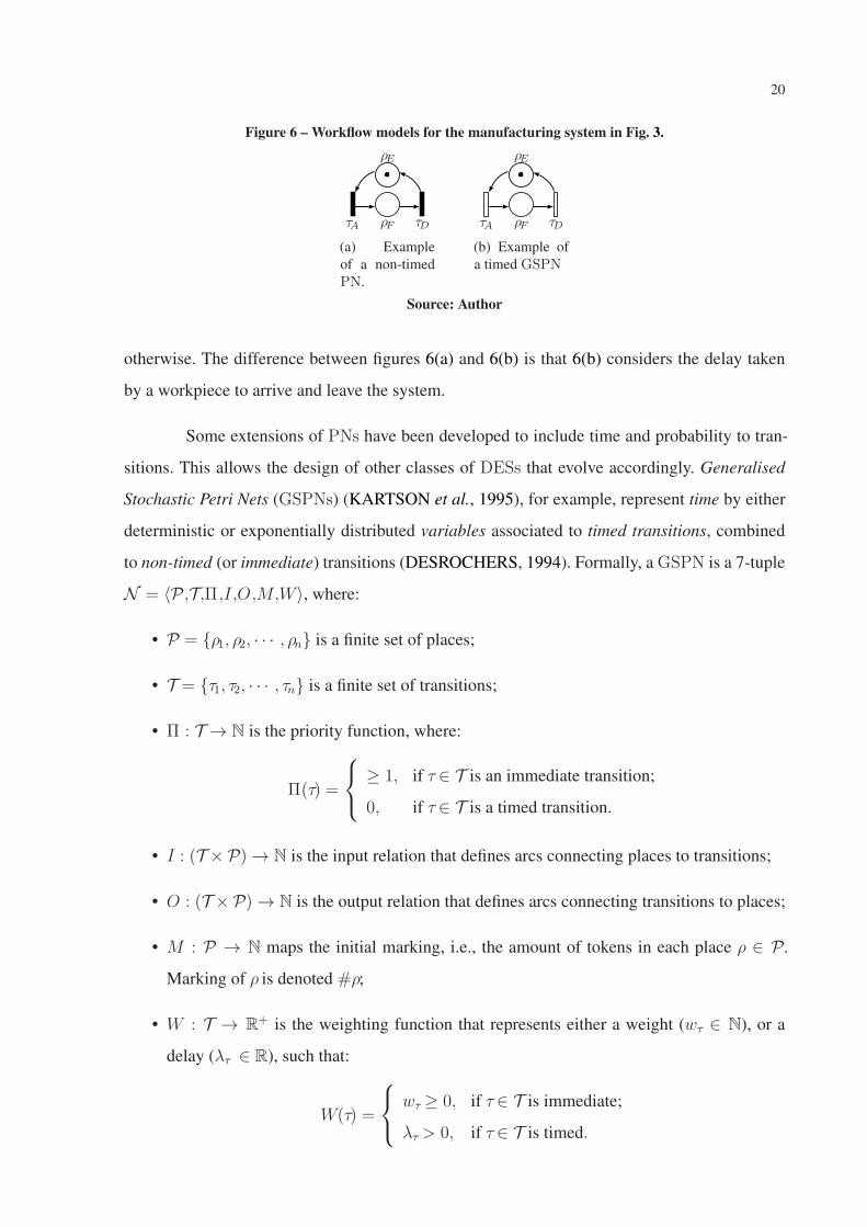
Example 5. Consider the manufacturing system in Fig. 3. Workpieces are delivered to a con-

veyor and moved to a static desk, for assembling with the robot X or Y . The PNs in Fig. 6

design workpieces flowing through the assembly desk.

Each model has two places, ρE and ρF , modelling respective the desk empty and full.

Transitions τA and τD model events of sensors signalling respectively arrivals and departures of

workpieces. In the initial state, the system is empty, therefore ρE is marked, and ρF is marked

20

Figure 6 – Workflow models for the manufacturing system in Fig. 3.

ρE

ρF τDτA

(a) Exampleof a non-timedPN.

ρE

ρF τDτA

(b) Example ofa timed GSPN

Source: Author

otherwise. The difference between figures 6(a) and 6(b) is that 6(b) considers the delay taken

by a workpiece to arrive and leave the system.

Some extensions of PNs have been developed to include time and probability to tran-

sitions. This allows the design of other classes of DESs that evolve accordingly. Generalised

Stochastic Petri Nets (GSPNs) (KARTSON et al., 1995), for example, represent time by either

deterministic or exponentially distributed variables associated to timed transitions, combined

to non-timed (or immediate) transitions (DESROCHERS, 1994). Formally, a GSPN is a 7-tuple

N = P ,T ,Π ,I,O,M,W, where:

• P = {ρ1, ρ2, · · · , ρn} is a finite set of places;

• T = {τ1, τ2, · · · , τn} is a finite set of transitions;

• Π : T → N is the priority function, where:

Π(τ) =

≥ 1, if τ ∈ T is an immediate transition;

0, if τ ∈ T is a timed transition.

• I : (T × P)→ N is the input relation that defines arcs connecting places to transitions;

• O : (T × P)→ N is the output relation that defines arcs connecting transitions to places;

• M : P → N maps the initial marking, i.e., the amount of tokens in each place ρ ∈ P.

Marking of ρ is denoted #ρ;

• W : T → R+ is the weighting function that represents either a weight (wτ ∈ N), or a

delay (λτ ∈ R), such that:

W(τ) =

wτ ≥ 0, if τ ∈ T is immediate;

λτ > 0, if τ ∈ T is timed.

21

The trajectory through the state-space of N depends on the pre and post conditions of

each transition τ, defined respectively by the sets←−τ = {ρ ∈ P | I(τ,ρ) > 0}, and −→τ = {ρ ∈

P | O(τ,ρ) > 0}; τ is said to be enabled in a marking M if, and only if, ∀ρ ∈ ←−τ , M(ρ) ≥

I(τ, ρ).

Therefore, a state of N changes when enabled transitions fire, and only they can fire.

Immediate transitions fire as soon as they get enabled, while timed transitions wait for a de-

lay λτ, that can be either deterministic (λdτ), or stochastic (λsτ), in this case associated with an

exponentially distributed delay. Delays of timed transitions are inversely proportional to the fre-

quency of firing, relation that defines the so-called firing rate. Timed transitions are additionally

associated with a serverType that defines the way multiple customers are handled. Infinite server

allows to attend tokens concurrently, while single server implies a sequential processing.

An important feature of N is being bounded. When a transition fires, it moves tokens

from input to output places. Therefore, the firing of τ ∈ T, enabled in the marking M , causes a

new marking M ′ such that ∀ρ ∈ (←−τ ∪ −→τ ), M ′(ρ) = M(ρ)− I(τ,ρ) + O(τ,ρ). N is said to be

bounded if it allows a finite number k > 0 of tokens in each place, ensuring a resulting finite

state-space.

When compared to other state-space-based approaches, such as Markov Chains,

GSPNs are shown to be more general, as they support either simulation or state-space analy-

sis. Furthermore, GSPNs allow to combine exponential transitions to form more complex time

distributions (DESROCHERS, 1994), broadening its applicability over DES problems.

22

4 PROPOSED WORKFLOW

Figure 7 – Layout of the proposed framework for distributed power generation.

Database Inf.System

M1 Mm

G11 G1

aGm

1 Gm

b

L1

L2

L3

BB1 BB2

GSPN

MPG

Source: Author

Consider the 3-layers workflow in Fig. 7. L1 represents the external main power grid

from where generation requests arrive periodically. L2 receives those requests and dispatches

the generation plan in L1, using an information system that also integrates data storage, optimi-

sation modules, and interface.

It is assumed that the layer L3 includes a finite number j = 1, · · · ,m of microgrids Mj ,

each one supporting a finite number of generators Gji , i = 1, · · · , g, such as wind, photovoltaic,

biomass, thermal, and small hydropower plants (SHPs). Furthermore, each microgrid Mj may

integrate a battery bank BBj , for energy storage. Microgrids Mj manipulate and report to the

other levels variables such as frequency, voltage, power, and resources availability.

Energy storage is important because it allows balancing variations in the renewable

production, in addition to covering the uncertainties in generation and consumption. With the

use of a battery bank, the system operator can implement load shifting, improve voltage and

frequency stability, reduce peak load, improve power quality, and postpone system updates

(BIAZARGHADIKOLAEI et al., 2019). Therefore, the ability to anticipate energy storage con-

ditions and their correlations are crucial for power systems planning.

In the next section, design and control of each layer is developed using supervisory

control. Then, we implement and communicate the elements through the layers for them to

cooperate based on policies to be further derived in Section 5.

23

4.1 MODELLING AND CONTROL

Seen as DESs, power generators can be of two types: the ones which controllably

deliver multiple levels of power (e.g., hydroelectric), and the ones which generate power ac-

cording to the uncontrollable availability of resources (e.g., wind and sun). These two classes

are modelled as follows.

4.1.1 Multiple-level generation modelling

The plant of a multiple-level power generator is formed by: a k-level generator, k

sensors, and a k-level power demand prescriber. For illustration, k is limited to 3, but this can

be straightforwardly extended to any finite number. The plant model of a generator is shown in

Fig. 8.

Figure 8 – Plant model Multiple-level power generator.G1: i1 i2 i3

d1 d2 d3

f ffr

p1 p2 p3

p0 p1 p2

G5:

G2: G3: G4:

s1 s2 s3

Source: Author

The FSM G1 models the generator; G2, G3, and G4 are associated with signals pro-

vided by sensors that report resources levels (e.g., water); and G5 models a power demand

prescriber, responsible for interfacing the generation level with the microgrid control.

Events it and dt, for t = 1, 2, 3, increase and decrease the generation level t; events f

and r model fault and recovery of G1; pt, for t = 0, 1, 2, 3, represents the power prescription;

and st, for t = 1, 2, 3, indicates the sensed level of resources. It is assumed that Σc = {it,dt,r}

and Σu = {pt,f,st}.

For the purpose of control, the specifications are:

Figure 9 – Specifications multiple-level power generator.E1: E2: E3:

E4: E5: E6:

p1

p1

p1

p1p1

p1

p2

p2

p2

p2p2

p2

p3

p3

p3

p0

p0

p0 i1,p0 i2,p1 i3,p2

d1,p1 d2,p2 d3,p3

Source: Author

24

• E1,2,3: avoid starting the generation levels i1,2,3 while there is no corresponding prescrip-

tion from p1,2,3;

• E4,5,6: avoid reducing the generation levels d3,2,1 while not prescribed from p2,1,0.

Fig. 9 shows the specification models. For example, E2 prohibits the event i2 (66.6%

of the total plant potential) unless it is explicitly prescribed (event p2) by the microgrid. The

same reasoning applies for the others.

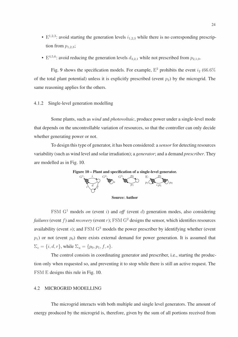
4.1.2 Single-level generation modelling

Some plants, such as wind and photovoltaic, produce power under a single-level mode

that depends on the uncontrollable variation of resources, so that the controller can only decide

whether generating power or not.

To design this type of generator, it has been considered: a sensor for detecting resources

variability (such as wind level and solar irradiation); a generator; and a demand prescriber. They

are modelled as in Fig. 10.

Figure 10 – Plant and specification of a single-level generator.G1: i

dfr

G3:

s p0

p0p0 E:G2:

p1 i,p1p1

Source: Author

FSM G1 models on (event i) and off (event d) generation modes, also considering

failures (event f ) and recovery (event r); FSMG2 designs the sensor, which identifies resources

availability (event s); and FSM G3 models the power prescriber by identifying whether (event

p1) or not (event p0) there exists external demand for power generation. It is assumed that

Σc = {i, d, r}, while Σu = {p0, p1, f, s}.

The control consists in coordinating generator and prescriber, i.e., starting the produc-

tion only when requested so, and preventing it to stop while there is still an active request. The

FSM E designs this rule in Fig. 10.

4.2 MICROGRID MODELLING

The microgrid interacts with both multiple and single level generators. The amount of

energy produced by the microgrid is, therefore, given by the sum of all portions received from

25

the associated generators. A microgrid model is shown in Fig. 11.

Figure 11 – Plant model of a microgrid.

0 1 2

M:

r f

f

dm

dmim

st

vt

Source: Author

Events im and dm model the start and stop of the microgrid; f and r model fault

and recovery; vt means the arrival of a prescription from the MPG; and st means that the

microgrid has been set up for the prescription vt. It is assumed that Σc = {dm, im, st, r}, while

Σu = {vt, f}.

Upon starting (transition 0im−→ 2), the microgrid sets up the production according to

its current prescription, which is initially empty. The conclusion of the set up is signalized by

the event st, which evolves the microgrid to the state 1 where it waits for any variation of the

prescription coming from the MPG. When it does (event vt), the microgrid returns to the state

2 and starts the production accordingly. This is achieved by sending an actuation instruction to

the generators under the microgrid, describing the amount of energy expected to be generated

by each of them.

The actuation scheme can be computed in such a way that it balances arguments such

as: (i) the level of resources reported by each generator; (ii) the power capacity of each generator;

(iii) the priority of use, which can be defined, for example, according to green policies; and

(iv) the time available to fulfil the demand in contrast with the number of generators and their

capacity. Later, in Section 5, we show a method to calibrate the actuators.

4.3 CONTROL SYNTHESIS

Let a microgrid be modelled by M1 with 4 states as in Fig. 11, under which two genera-

tors operate. The first is of the type multiple-level and it is modelled by the plant G11 =

5p=1 G

p

(Fig. 8), specified by E11 =

6q=1 E

q (Fig. 9). Then, for K11 = G1

1E11, the controller supC(K1

1,G11)

is modelled by V11 with 105 reachable states.

The second generator is single-level type and it has plant G12 =

3p=1 G

p and specifica-

tion E12 = E as in Fig. 10. For K1

2 = G12 E

12, the controller supC(K1

2,G12) is modelled by V1

2

with 9 states.

26

M1, V11, and V1

2 can then be translated to implementable code and deployed in hard-

ware, e.g., a microcontrolled system. Each controller (V11 and V1

2) can be further communicated

with M1, according to the workflow in Fig. 7, so that they can report their status and receive

customised prescriptions for power generation, which is approached next.

27

5 PETRI NET-BASED CUSTOMISATION

In addition to the event-based control, elements of a microgrid are expected to coop-

erate toward common goals. In this paper, cooperation policies are discovered by simulating

GSPNs that model power generators. A GSPN that represents a general power generator is

shown in Fig. 12.

Figure 12 – A basic GSPN model for a power generator.RP:

Wτ1 τ2

λ1 λ2

Source: Author

P is composed of two places, R and W, connected by the timed transitions τ1 and τ2. R

quantifies the resources (tokens) available for power generation, while W models the working

place, i.e., energy production. τ1 and τ2 impose state transitions to P using tokens in R and W,

and firing delays.

Transition τ1 fires at a rate 1/λ1, in which λ1 is its delay. τ2 has a firing rate of 1/λ2,

for a delay λ2 representing the time took by the generator to produce a given portion of energy.

Here, #R is set to 1 in order to model generators producing sequentially, one energy unit at a

time, after a delay λ2 ≥ λ1. Later, multiple generators are designed and (#R) is set accordingly.

Also, it has been assumed a Single Server firing policy for τ2 (see Section 3.3), while later this

may have to be replaced by the Infinite Server policy.

From P, multiple generation profiles can be reproduced by simply varying λ2, or by

setting workflows that connect multiple P models. This allows to capture distinct plant profiles

and environmental changes, such as panel shading or wind intensity, when it is the case. Remark

that these events are reported by the sensors that follow generators in the level L3 of Fig. 7. They

are used to calculate the parameters for λ2, as follows:

λ2 =∆RM

(RM −min(RM))· T , (1)

where ∆RM = max(RM) − min(RM) defines the range of resource level within which the

generator can produce; RM is the real (measured) resource; and T is the observation interval. By

28

feeding P with different values for λ2, one can simulate, for example, photovoltaic generation,

as exploited next.

5.1 A CASE STUDY ON PHOTOVOLTAIC GENERATION

The basic principle of PV technology is to use solar radiation (S) over panel cells

to generate electrical current (VILLALVA et al., 2009). However, there are many variables

involved in this process that interfere on the power generation performance (KING et al., 1997).

For example, the incidence of S is variable; each panel has a constant capacity; panels can be

clustered differently; each part of a power plant can receive different rate of S; etc.

Therefore, when applying P as in Fig. 12 to model a solar panel (denote PS), these

variables have to be considered. In the model that follows, they are used only to calculate the

delay λ2. When a token is in R waiting τ1 to fire, this means the absorption of solar radiation

over the panel, which here is assumed to be immediate, so λ1 is set to 1. When the token moves

to W and waits τ2 to fire, after a delay λ2 ≥ λ1, this means the time took by the panel to generate

a given portion of energy as a function of variable solar incidence indexes. Therefore, λ2 can be

calculated as in Eq. (1), for R = S. The result is the set of input parameters presented in Tab. 1,

which can be used to feed a GSPN PS and vary λ2.

Remark 1. As λ2 may change very frequently as a function of the solar incidence, the mean

amount of energy produced within a certain period of time is unclear from the panel spec-

ification, benchmarks or analytic processing. Thus, our intention here is to anticipate power

generation under variability, specially in the context of a more general microgrid system as in

Section 6.

Table 1 – Input parameters derivation for λ2.

Hour S (W/m2) λ2 (s) Hour S (W/m2) λ2 (s)10:00 190.81 9.9108 16:00 1005.83 1.011:00 401.94 2.9807 17:00 900.56 1.010612:00 716.94 1.4588 18:00 725.00 1.440013:00 890.28 1.1388 19:00 401.67 2.983414:00 1004.17 1.0 20:00 149.08 18.337415:00 1043.89 1.0

Tab. 1 uses an illustrative sample of solar radiation collected from a meteorological

station in Brazil. The second column presents the radiation (S) measured for each period under

observation (first column), while the third column shows the time, in seconds, to be assigned to

29

λ2 to represent the panel production under the corresponding radiation S (calculated as in Eq.

(1)). As the whether conditions are good, the generation is expected to reach the full potential

of the PV panel.

Remark 2. In Tab. 1, the greater the delay λ2, the fewer the amount of generated power, and the

longer the time to generate it. For example, at 10 o’clock, S = 190.81W/m2 requires 9.9108s

to generate the same amount of energy produced at 14 o’clock within 1s. Between 14 and 16

the system reaches the maximum potential, which is bounded by the panel capacity.

For illustration, assume that PS is a panel that generates 330W (Watts) per sec-

ond (1s) under maximum S rate (max(S)) and under mean temperature of 25 Celsius de-

grees. The acceptable range for photovoltaic production is between min(S) = 100W/m2 and

max(S) = 1000W/m2, which gives ∆S = 900W/m2. Assume also that T is associated with

1s, meaning the immediate generation of the panel full power. When S ≥ 1000, the delay λ2

is set to min(λ2) = 1, which returns the maximum performance production. Also λ1 is set to

min(λ2), as one aims to observe variations in λ2 only.

The following question can now be introduced.

Question 1. Consider a panel with maximal performance max(S) is 350W each 1s. By making

λ2 = 1, the value of each token after λ2 is 350W . However, any variation of S makes 1s

no longer enough to generate 350W and one wonders either what is the amount of energy

generated within the same 1s, or when will the system be able to generate 350W under variable

S.

Model PS can then be simulated to answer this type of question, as follows.

5.1.1 Photovoltaic simulation and analysis

After feeding the model PS with the parameters in Tab. 1, it is simulated to compute

metrics of interest. All simulations in this paper use the Stationary Simulation Standard al-

gorithm implemented by the TimeNet tool (ZIMMERMANN; KNOKE, 2007), considering a

confidence level of 95%, and relative error of 10%.

Then, τ2 was increasingly varied to estimate the system utilisation:

U(W) = (#W ≥ 0) , (2)

30

meaning the probability of how busy the system is likely to be; and the system response time:

R(W) = (E(W)) · (1/λ2) , (3)

meaning how long the system takes to produce certain amount of energy, for

E(W) = (#W) , (4)

capturing the mean expectation of marking in the place W, and R confronting this expectation

further with the frequency of firing, which returns the mean waiting time in W.

By using the formulaR (W), one can provide answers for the Question 1, as it maps the

performance estimated for a PV panel when operating under variable incidence of resources. It

remains to know whether this estimation coincides with the performance that would result from

the real panel. In Fig. 13, the real performance is obtained from the panel specification, but later,

in Section 6, it will be measure directly from the real installed system.

Figure 13 – Performance evaluation of a photovoltaic panel under variable resources.

10h00 12h00 14h00 16h00 18h00 20h00

0

100

200

300

400Estimated

Measured

Observation Time

Ene

rgy

(Wh)

When S ≥ 1000W/m2 (between 14 and 16 o’clock), both estimation and specifica-

tion suggest the full 350W generation within 1s. However, the performance is of only 35.3W

(real) and 36.8W (estimated) when S = 190.81W/m2; improving to 243.1W (real) and 259.7W

(estimated) when S = 725W/m2.

Other perspective for Question 1 is: which is the amount of energy estimated to be

obtained between 11 and 12 o’clock, which turns out to be 128.4W . One may also wonder how

long the system takes to generate 1000W , if S is 401.94W/m2, for which simulation informs

2.9807s.

With these estimations on hands, the control level L2 can be informed whether or not

the available microgrids can reach the target production, and whether or not a new dispatch

plan is needed for the microgrids. The advantage of having these information in advance is

31

that reconfiguration can be done preventively, without the need for measuring the real system.

Measures tend to be more precise in comparison with simulations, but they allow only for

reactive engineering, while simulations project predictive engineering.

The estimations in Fig. 13 have accuracy of 95.9% with respect to the real system

behaviour. This suggests that the model can now be extended and tested under more complex,

variable, and larger scenarios. In the following, the model is tested in the context of a real plant.

A single panel is again used as the basic evaluation, which is then extended to a set (string) of

combined panels. Other components inside a microgrid are also integrated to the model, such

as storage facilities, loads, and external power supplier.

32

6 CASE STUDY INVOLVING A REAL POWER PLANT

This section applies our model to determine the performance of a real PV plant. Sec-

tion 6.1 presents the system setup, which is assessed first as a group of panels in Section 6.1, and

as a microgrid in Section 6.2. Simulation results for both scenarios are respectively discussed

in sections 6.1.1 and 6.2.2.

6.1 REAL SYSTEM SETUP

Figure 14 – Partial layout of the real photovoltaic system at UTFPR.

Source: UTFPR.

The following experiments are conducted over a 420kW photovoltaic system installed

at the Federal University of Technology Paraná (UTFPR), in Brazil. The plant is composed of

1237 panels distributed over different block buildings. The panels of each block form strings that

are connected to 7 inverters that transform continuous to alternate power. Each string is linked to

a Maximum Power Point Tracker (MPPT), responsible for maintaining the power coming from

the panel, through the current control. For the sake of brevity, a single inverter was chosen for

illustration. It is composed of 8 strings of panels, 156 panels in total of 340W each, as shown

in Tab. 2.

The irradiation data, obtained from the sensors positioned close to this inverter, are

used to derive (by the Equation (1)) the input parameters for the GSPN model in Fig. 12. The

collected data can be found in Tab. 3.

33

Table 2 – Plant potential and distribution.MPPT ID String ID Number of panels Capacity (W )MPPT 1 F - 1 22 7480

F - 2 22 7480MPPT 2 F - 3 17 5780MPPT 3 F - 4 22 7480

F - 5 22 7480MPPT 4 F - 6 17 5780

F - 7 17 5780MPPT 5 F - 8 17 5780TOTAL 156 53040

Table 3 – Input parameters of the model.

Hour S(W/m2) λ2 (s) Hour S(W/m2) λ2 (s) Hour S(W/m2) λ2 (s)07:30 181.4 11.0565 11:00 778.3 1.3268 14:15 757.9 1.368007:45 185.5 10.5263 11:15 794.0 1.2968 14:30 189.6 10.044608:00 220.0 7.5000 11:30 806.4 1.2741 14:45 635.6 1.680408:15 347.8 3.6320 11:45 814.4 1.2598 15:00 649.4 1.638208:30 404.0 2.9605 12:00 817.7 1.2540 15:15 586.4 1.850308:45 427.5 2.7481 12:15 812.7 1.2628 15:30 507.6 2.208009:00 475.4 2.3974 12:15 812.7 1.2628 15:45 461.5 2.489609:15 530.9 2.0887 12:30 802.9 1.2804 16:00 240.7 6.396609:30 572.2 1.9060 12:45 800.2 1.2853 16:15 488.0 2.319609:45 616.1 1.7438 13:00 793.3 1.298 16:30 425.8 2.762410:00 660.5 1.6057 13:15 793.7 1.2974 16:45 332.0 3.879310:15 694.3 1.5144 13:30 350.3 3.5957 17:00 258.2 5.689010:30 726.5 1.4366 13:45 776.6 1.3302 17:15 167.0 13.432810:45 756.9 1.3701 14:00 767.1 1.3491 17:30 121.8 41.2844

6.1.1 Model simulation and analysis

The model is then simulated to anticipate the performance possibly achieved by the

panels when in production under variable resources. The simulations were further separated

into the three steps that follow:

(i) The panel performance is estimated using the GSPN model;

(ii) The real performance resulting from the inverter containing the 156 panels is measured

in the real plant;

(iii) The dynamic generation system is further reproduces for comparison using the Matlab

Simulink Toolbox.

The samples are then compared and Fig. 15 shows the results.

Inspection shows that the performance estimated by the GSPN model has a proximity

of 86% with respect to the real plant performance, in both tests, while the Simulink/Matlab

model returns a proximity of 81% compared to the real system. The formula used to approxi-

34

Figure 15 – Estimated versus measured power generations

06h00 08h00 10h00 12h00 14h00 16h00 18h00

Observation Time

0

50

100

150

200

250

300Simulink

Measured

GSPN

Ene

rgy

(Wh)

(a) Analysis of 1 module.

06h00 08h00 10h00 12h00 14h00 16h00 18h00

Observation Time

0

1

2

3

4

104

Simulink

Measured

GSPN

Ene

rgy

(Wh)

(b) Analysis of 156 panels.

mate the curves is accuracy:

E =xm − xe

xm

, (5)

in which xm is the measured, and xe is the estimated (GSPN and Simulink) values. The result

of Eq. (5) are deducted from 100%, leading to the accuracies for either GSPN or Simulink.

Remark that estimations for strings have a non-additive nature in comparison with

single-panel estimations, as the conditions over each part of the string may differ. As such, there

are many possible noises disturbing the inverter performance. In our model, this is captured by

collecting input parameters for each panel that compose the string (similar to the single-panel

case) and then deriving the input parameters for the entire string, based on mean and standard

deviation analysis. In case the standard deviation is significant, the model can be split into the

string to isolate more unstable sectors of production. Otherwise, the standard deviation may be

neglected, as this is shown to be minor and will not affect the result considerably.

It remains to shown whether our dynamic model can serve for more general decision

makings, in the context of a microgrid management, as follows.

6.2 MICROGRID MODELLING

Departing from the generator model in Fig. 12, one can now organise a plug-and-play

like model that allows engineers to reconfigure and simulate specific parts of a microgrid, or

vary the number and specifications of its components, such as energy sources, battery banks,

and load profiles. The microgrid model proposed in this paper is shown in Fig. 16.

Model M includes 4 basic blocks, intended to design 4 different microgrid components:

35

A1

Ai

B1

C1

Bi

Ci

WB

RB RL

WL

WSτS

τB τL

B L

P1

Pn

S

.

.

.

M: P

Figure 16 – Proposed GSPN to design plug-and-play microgrid components.

Source: Author

source (generator), storage (battery bank), load (consumption), and surplus (simulating the

MPG interaction). The energy provided by the multiple sources (denoted by Pi, i = 1, · · · ,n)

are channelled either towards a battery bank (block B), in case it has capacity enough for charg-

ing, or towards a surplus resource (block S), otherwise. From block B the energy serves to a

load simulator (block L), which represents the microgrid consumption.

Each model Pi, i = 1, · · · ,n, has a function equivalent to the model P in Fig. 12. For

the storage in B, the place RB quantifies the remaining storage level (#RB), while λB defines the

network rate for the block B, which is directly linked with the input of the block L. Similarly,

L has a place RL to quantify the amount of energy consumed by the microgrid (#RL), while the

exit point λL defines its consumption rate. Finally, λS in S models the rate of power injection

into the MPG, which results from tokens inserted in the place WS when the power generation

is greater than the storage capacity.

While some parameters in M are generic, others depend on specific features collected

from the infrastructure to be assessed. In the following one shows how they can be defined.

6.2.1 Input parameters for M

Intuitively, when the battery bank B reaches its saturation point, i.e., the symbolic

amount of power carried by one token is greater than the available resources in B, the power de-

livered by P has to be redirected to the surplus block S. In the on grid mode, this represents the

injection of power in the MPG, while in the off-grid model this means, for example, suspending

generation as the saturation point has been reached.

For the purpose of modelling the power switching from B to S, guard formulas are

implemented to test Boolean conditions over the arcs that connect P to B and S, as shown in

36

Tab. 4.

Table 4 – Arc conditions for the microgrid model.Arcs Condition

A1 and Ai IF((#RB) <= 1):0 ELSE 1B1 and Bi IF((#RB) <= 1):0 ELSE 1C1 and Ci IF((#RB) <= 1):1 ELSE 0

It is also important to consider that a single microgrid may be composed of several gen-

erators, which differ in their power generation potential, delivering distinct amounts of energy

to the microgrid. In terms of modelling, this means that each token may carry different values

of energy, depending on where it came from. One option to address this feature is by weighting

the arcs that depart from the generator according to the generator potential, i.e., each generator

(or group of similar ones) delivers a distinct amount of energy to the grid. A fancier possibility

is to take advantage from the Infinity Server property of timed transitions (see definition in Sec-

tion 3) to establish customised parallel processing resources for each generator model, which

will equivalently balance different power generation profiles. Therefore, let:

• #Ri be the marking of Ri, for each generator Pi, i = 1, · · · , n;

• Pti be the maximum power capacity of the generator Pi (in Watts (W )), such that the

amount of power in M is Pt =n

i=1

Pi; and

• GCD(x,y) be the Greatest Common Divisor of the integers x and y.

Then, the parallel processing in Pi is

#Ri =Pti

GCD(Pt1, · · · ,Ptn). (6)

In this way, #Ri represents the individual impact caused by each Pi over the microgrid

potential Pt. For example, let P1 and P2 be two generation subsystems, such that P1 includes

100 PV panels with a capacity of 350W each, while P2 includes 50 PV panels with a capacity

of 280 W each.

Then, Pt1 = 100 · 350 = 35000W , and Pt2 = 50 · 280 = 14000W . By

GCD(35000,14000) = 7000, it follows that #R1 = Pt1/7000 = 35000/7000 = 5 and

#R2 = Pt2/7000 = 14000/7000 = 2. In summary, P1 can process 5 tokens in parallel, which

means 5 · 7000 = 35000W to the microgrid. Similarly, P2 can process 2 tokens in parallel,

which means providing 2 · 7000 = 14000W .

37

6.2.2 Microgrid simulations and analysis

From the model in Fig. 16, an important matter is to anticipate for engineers the vari-

able relationship among P, B, L, and S. This may not be so easy to inform empirically or

analytically, as the system variabilities cause non-addictive effects over the microgrid. Alter-

natively, the microgrid model in Fig. 16 can applied over the real PV plant, simulated, and

compared with the real power generation performance. Model M in Fig. 17 is a version of the

model Fig. 16, adapted to represent this particular case study.

A

B

C

WB

RB RL

WL

WS

R

W

τS

τB τLτ1 τ2

M:

Figure 17 – GSPN model for the case study.

Source: Author

The same version of the plant is used, i.e., one inverter connected to 156 panels of

340W . It delivers energy to a battery bank (place WB), whose capacity (#RB) one aims to vary

for the storage planning. The blocks L and S are also considered and used to estimate the level

of consumption and surplus that result when the model M is reconfigured variably.

In the following, the focus is on anticipating the amount of energy produced by the 156

panels, considering two different scenarios: with and without microgrid consumption. Further-

more, it is considered variable sizes for the battery bank infrastructure. The following setup is

assumed:

• #R: technically, #R results from Eq. (6), i.e.,

#R =156 · 340

1= 53040W = 53kW.

In this experiment, only 340W panels are considered. Thus, GCD(340) = 1 implies that

#R may be replaced by #R = 156, i.e., by the number of panels that compose the inverter,

instead of their capacity. In this case, the semantics carried by each token means 340W

of power, leading to the equivalent capacity of 340 · 156 = 53040W . Remark that, when

#R = 53kW , each token carries 1kW , while in #R = 53040W each token means 1W ,

and they all equivalent to design #R.

38

• λ1 = 1 = λL = λS: for λ1 the same notion as in Fig. 12 is used, i.e., it is fixed to 1, so that

one can vary only the time took by the panels to produce, i.e., λ2 ≥ λ1. Similar purpose

applies for λL and λS , which are not varied;

• λ2: this delay is defined in Tab. 3, which includes the irradiation data that, in conjunction

with the Eq. (1), allows to compute variable delays for λ2. In the experiments that follow,

for the sake of brevity, λ2 is not varied for all the intervals in Tab. 3. Instead, it is illustrated

only for the solar peak, although other variations can be straightforwardly set. In this way,

for the time observation of 1 hour (T = 1), under the solar peak, it follows from Eq. (1)

that

λ2 =(1000− 100)

(1000− 100)· 1 = 1 .

In order to impose variability to the model, so that it can be measured accordingly, the

following parameters are tested:

• The delay λB was varied into 1s and 0.1s, to model two profiles of power injection in

WL . Remark that the lower the delay λB , the greater the rate in L, i.e., the greater the

consumption.

• The marking #RL was varied into 50, 100, and 150, to represent the amount of power to

be absorbed in parallel by the microgrid, ranging from 50 · 340 = 17000W to 150 · 340 =

53040W .

• The marking #RB considers the range 20, 40, 60, 80, 100, 120, 140, and 156. This sim-

ulates variations in the storage capacity. As each token corresponds to 340W , then the

storage capacity ranges from 20 · 340 = 6800W to 156 · 340 = 53040W , coinciding at

the upper bound with the total plant capacity.

After feeding the model with parameters, it was simulated under variability. The met-

rics to be estimated are the same as in equations (3) and (4), but this time applied to the place

WB , i.e., to the battery bank, which is the counterpart of the surplus WS , so that this analysis

allows to observe their behaviour under variability. The TimeNet setup is also the same as in

section 5.1.1, and the question to be answered can be stated as follows.

Question 2. For a load consumption (#RL) varying from 17000W to 53040W , which is the

battery bank dimensioning that accommodates the residual amount of energy left over from

such a generation profile with variable load?

39

Fig. 18 and Fig. 19 show possible answers provided by the model.

Figure 18 – Storage dimensioning (#RB ) under three load profiles (#RL ): 50 to 150 tokens – 17000W to53040W , with λB = 1s.

20 40 60 80 100 120 140 160

0

1000

2000

3000

4000

5000

67%

14%53%

10%

#RL = 50#RL = 100#RL = 150

Storage facility capacity (#RB )

Ene

rgy

(Wh)

In Fig. 18, the lower the load potential (#RL), the greater the residual energy to be

stored (#RB). For example, when #RL = 50 (low consumption profile), a storage facility of

20 tokens (20 · 340 = 6800W ) would be 67% full in average, while an upgraded version of 60

tokens (60 · 340 = 20400W ) would be only 14% occupied. In comparison, when #RL = 150

(high consumption profile), the same storage facility of 20 tokens would be about 53% occupied,

while the same upgrade to 60 tokens would lead to only 10% occupation.

As expected, the storage level decreasing is more substantial when #RB < #RL

(before the dashed line), in which cases the consumption is higher and more tokens are moved

from RB to RL . Otherwise, when #RB ≥ #RL , more tokens are retained in RB , and the storage

level starts to stabilise.

This tendency is even more perceptible when the access to the load module L (λB in

τB) is reconfigured to increase its firing rate from 1/λB = 1s to 1/λB = 0.1s. In practice, this

means that the load profile (with the same 50, 100, and 150 parallel tokens) will now be about

10 times more frequent, which tends to consume the storage facility much faster.

As expected, Fig. 19 shows that the battery bank level decreases much faster in compar-

ison with Fig. 18. For example, when #RL = 50 (low consumption profile), a storage facility

of 20 tokens would now be only 26% occupied, against 67% of the previous experiment. When

#RL = 150 (high consumption profile), the same storage facility of 20 tokens would be only

7% occupied, against the 50% occupation of the previous experiment. An upgrade to 60 tokens

of storage (20400W ) keeps the stable 7% occupation under the high consumption rate, against

the previous 14%.

Actually the entire experiment with #RL = 150 keeps a stable storage index below

40

20 40 60 80 100 120 140 160

0

500

1000

1500

26%

7%

#RL = 50#RL = 100#RL = 150

Storage facility capacity (#RB )E

nerg

y(W

h)

Figure 19 – Storage dimensioning (#RB ) under three load profiles (#RL ): 50 to 150 tokens – 17000W to53040W , with λB = 0.1s.

10%, which means that practically the total amount of energy that will be produced, will be con-

sumed. The other two load profiles, #RL = 100 and #RL = 50, accumulate energy resources

when #RB is less than about 100 tokens, after which the three load profiles lead to similar,

stable, but very low, storage level.

There were no similar results in the literature that could be compared to ours, as we did

using Simulink in Section 6.1.1. We believe this is because of the concurrent nature of microgrid

components and their variabilities, which makes it hard to be reproduced by modelling and

results in a large number of combinations and possible states, complexifying similar analysis.

6.3 EXAMPLE OF COOPERATIVE DISTRIBUTION

Consider that the evaluated PV plant is part of a larger smart grid, which delivers

energy cooperatively to the main power grid, through a distribution system. The system has the

following infrastructure:

• M1 is a microgrid composed of 10 wind turbines of 6kW each;

• M2 is the evaluated PV microgrid;

• M3 is a Small Hydroelectric Plant (SHP), with a potential for 500kW .

For a request received from the main power grid, let us say, at 11 : 30, to deliver

125.0kW for the next 1 hour, what the prescription recommended by the system operator for

dispatching those three power plants?

Intuitively, the SHP itself can provide the total amount of power. However, water re-

sources are always to be saved, considering their scarcity, environmental impact, and the prob-

41

ability of new requests in the near future. Furthermore, water uses to impose a chained effect

over other plants along the course of a river, so it cannot be arbitrarily used.

Therefore, the previous question can be reintroduced this way: for a request of

125.0kW , for the next 1 hour, what would be the amount of energy produced from wind and

sun resources, so that the system operator could dispatch the SHP (or other stable source) only

to fulfil the remaining amount?

Assume that a 6kW turbine is capable of generating about 3.83kW in an hour, with a

wind incidence of, for example, 5.4m/s (this is only an assumption, as wind generation has not

yet been considered in our model). Thus, M1 would be capable of delivering 38.3kW . From

the model, it is known that M2 delivers approximately 42kW . Therefore, the remaining amount

to be dispatched from M3 is 61kW . This means that wind and PV units deliver approximately

18.4% and 33.6% (i.e., 52%) of the total request, and they act cooperatively to fulfil the expected

power generation.

42

7 CONCLUSIONS AND PERSPECTIVES

In this paper, components of a PV power system are seen as event-driven entities that

are modelled using GSPNs. The advantage of this approaches relies on the fact that a GSPN

can be simulated to anticipate performance metrics for the system, which becomes a powerful

tool for engineer to plan the system, either to construct it, to expand an existing system, or to

regulate energy trading contracts on the market.

The model has been tested against a real PV system. Its estimations were capable of

following the real system performance with an accuracy of approximately 86%. Afterwards,

the PV generation system was integrated with other components of a larger microgrid and the

corresponding modelling extensions are provided. Results show that it is possible to anticipate

resources planning decisions at the design time, which tends to be a valuable tool for predictive

engineering in distributed power generation systems.

Future researches will focus on user interfacing and integration with generation control

systems for automatic support for optimisation. Furthermore, we aim to add other types of

generation profiles to the microgrid model, such as wind plants, as well as establishing new

mechanisms for discovering cooperative policies for power generation systems, in the context

of the cyber-physical energy grid (SUPERGRID, 2021) of the future.

43

REFERENCES

ALAM, Mahamad Nabab; CHAKRABARTI, Saikat; LIANG, Xiaodong. A benchmark testsystem for networked microgrids. IEEE Trans. on Industrial Informatics, IEEE, v. 16, n. 10,p. 6217–6230, 2020.

ASMUS, Peter. Microgrids, virtual power plants and our distributed energy future. TheElectricity Journal, Elsevier, v. 23, n. 10, p. 72–82, 2010.

BIAZARGHADIKOLAEI, Milad; SHAHABI, Majid; BARFOROUSHI, Taghi. Expansionplanning of energy storages in microgrid under uncertainties and demand response. Int. Trans.on Electrical Energy Systems, Wiley Online Library, v. 29, n. 11, p. e12110, 2019.

CASSANDRAS, C. G.; LAFORTUNE, S. Introduction to Discrete Event Systems. [S.l.]:Springer Science, 2008.

CASSETTARI, Lucia; BENDATO, Ilaria; MOSCA, Marco; MOSCA, Roberto. EnergyResources Intelligent Management using on line real-time simulation: A decision support toolfor sustainable manufacturing. Applied Energy, v. 190, p. 841–851, 2017.

CATALãO, João PS. Smart and sustainable power systems: operations, planning, andeconomics of insular electricity grids. [S.l.]: CRC Press, 2017.

CHAMORRO, HR; ORDONEZ, CA; JIMENEZ, JF. Coordinated control based Petri Nets forMicrogrids including wind farms. In: IEEE. 2012 IEEE Power Electronics and Machines inWind Applications. [S.l.], 2012. p. 1–6.

DADFAR, Sajjad; WAKIL, Karzan; KHAKSAR, Mehrdad; REZVANI, Alireza; MIVEH,Mohammad Reza; GANDOMKAR, Majid. Enhanced control strategies for a hybridbattery/photovoltaic system using FGS-PID in grid-connected mode. Int. Journal ofHydrogen Energy, Elsevier, v. 44, n. 29, p. 14642–14660, 2019.

DENHOLM, P.; ELA, E.; KIRBY, B.; MILLIGAN, M. Role of Energy Storage withRenewable Electricity Generation. [S.l.], 2010.

DESROCHERS, A. A. Applications of Petri Nets in Manufacturing Systems: Modeling,Control and Performance Analysis. [S.l.]: IEEE Press, 1994.

DJELLOULI, Abderrahmane; LAKDJA, Fatiha; RACHID, Meziane. Control and Managementof Hybrid Renewable Energy System. In: SPRINGER. Int. Conf. on Smart Innovation,Ergonomics and Applied Human Factors. [S.l.], 2019. p. 1–10.

44

FAN, Yang; MING-TIAN, Fan; ZU-PING, Zhang. China mv distribution network benchmarkfor network integrated of renewable and distributed energy resources. In: IEEE. China Int.Conf. on Electricity Distribution. [S.l.], 2010. p. 1–7.

FARHANGI, Hassan; JOOS, Geza. Microgrid benchmarks. [S.l.]: Wiley-IEEE Press, 2019.

GELEN, Ayetül; GELEN, Gökhan; BıçAK, Aykut. Supervisory controller design for reactivepower compensation. European Journal of Science and Technology, 11 2020.

GHASAEI, Arman; ZHANG, Zhi Jin; WONHAM, W Murray; IRAVANI, Reza. A Discrete-Event Supervisory Control for the AC Microgrid. IEEE Trans. on Power Delivery, IEEE,p. 1–1, 2020.

HARITZA, Camblong; OCTAVIAN, Curea; AITOR, Etxeberria; ALVARO, Llaria; AMéLIE,Hacala Perret. Research experimental platforms to study microgrids issues. Int. Journal onInteractive Design and Manufacturing (IJIDeM), Springer, v. 10, n. 1, p. 59–71, 2016.

HATZIARGYRIOU, Nikos; ASANO, Hiroshi; IRAVANI, Reza; MARNAY, Chris. Microgrids.IEEE Power and Energy Magazine, IEEE, v. 5, n. 4, p. 78–94, 2007.

IEA, International Energy Agency. World Energy Balances: Overview. [S.l.], 2018. Availableat: https://shorturl.at/fuL46. Accessed on: 01 abr. 2019.

JANA, Debashis; CHAKRABORTY, Niladri. Generalized stochastic Petri nets for uncertainrenewable-based hybrid generation and load in a microgrid system. Int. Trans. on ElectricalEnergy Systems, Wiley Online Library, v. 30, n. 4, p. e12195, 2020.

KARTSON, D.; BALBO, G.; DONATELLI, S.; FRANCESCHINIS, G.; CONTE, Giuseppe.Modelling with Generalized Stochastic Petri Nets. [S.l.]: Wiley & Sons, 1995.

KING, D. L.; KRATOCHVIL, J. A.; BOYSON, W. E. Measuring solar spectral and angle-of-incidence effects on photovoltaic modules and solar irradiance sensors. In: PhotovoltaicSpecialists Conference. [S.l.: s.n.], 1997. p. 1113–1116.

KOTSAMPOPOULOS, Panos; LAGOS, Dimitris; HATZIARGYRIOU, Nikos; FARUQUE,M Omar; LAUSS, Georg; NZIMAKO, Onyi; FORSYTH, Paul; STEURER, Michael; PONCI,F; MONTI, A et al. A benchmark system for hardware-in-the-loop testing of distributedenergy resources. IEEE Power and Energy Technology Systems Journal, IEEE, v. 5, n. 3, p.94–103, 2018.

LASSETER, Robert H; PIAGI, Paolo. Microgrid: A conceptual solution. In: IEEE. PowerElectronics Specialists Conference. [S.l.], 2004. v. 6, p. 4285–4291.

45

LU, Xiaoyu; ZHOU, MengChu; AMMARI, Ahmed Chiheb; JI, Jingchu. Hybrid petri netsfor modeling and analysis of microgrid systems. IEEE/CAA Journal of Automatica Sinica,IEEE, v. 3, n. 4, p. 349–356, 2016.

MIRSAEIDI, Sohrab; SAID, Dalila Mat; MUSTAFA, Mohd Wazir; HABIBUDDIN,Mohd Hafiz; GHAFFARI, Kimia. Progress and problems in micro-grid protection schemes.Renewable and Sustainable Energy Reviews, Elsevier, v. 37, p. 834–839, 2014.

MURATA, T. Petri Nets: Properties, Analysis and Applications. Proceedings of the IEEE,IEEE, v. 77, p. 541–580, 1989.

NAVERSEN, Christian Oyn; FARAHMAND, Hossein; HELSETH, Arild; CATALãO, João.Hydrothermal scheduling in the continuous-time framework. ArXiv, p. arXiv–1912, 2019.

NEHRIR, MH; WANG, Caisheng; STRUNZ, K; AKI, H; RAMAKUMAR, R; BING, J; MIAO,Zhixhin; SALAMEH, Z. A review of hybrid renewable/alternative energy systems for electricpower generation: Configurations, control, and applications. IEEE Trans. on SustainableEnergy, IEEE, v. 2, n. 4, p. 392–403, 2011.

OLIVARES, Daniel E; CAÑIZARES, Claudio A; KAZERANI, Mehrdad. A centralized energymanagement system for isolated microgrids. IEEE Trans. on Smart Grid, IEEE, v. 5, n. 4, p.1864–1875, 2014.

PARVANIA, Masood; SCAGLIONE, Anna. Unit commitment with continuous-timegeneration and ramping trajectory models. IEEE Trans. on Power Systems, IEEE, v. 31, n. 4,p. 3169–3178, 2015.

PATHAK, Pawan Kumar; YADAV, Anil Kumar. Design of battery charging circuit throughintelligent MPPT using SPV system. Solar Energy, Elsevier, v. 178, p. 79–89, 2019.

PAULISTA, Cássio Rangel; PEIXOTO, Túlio Almeida; RANGEL, João José de Assis.Modeling and discrete event simulation in industrial systems considering consumption andelectrical energy generation. Journal of Cleaner Production, Elsevier, v. 224, p. 864–880,2019.

RAMADGE, Peter JG; WONHAM, W Murray. The control of discrete event systems.Proceedings of the IEEE, IEEE, v. 77, n. 1, p. 81–98, 1989.

RODRÍGUEZ, Miguel Romero; DELPOUX, Romain; PIÉTRAC, Laurent; DAI, Jing;BENCHAIB, Abdelkrim; NIEL, Eric. Supervisory control for high-voltage direct currenttransmission systems. IFAC-PapersOnLine, Elsevier, v. 50, n. 1, p. 12326–12332, 2017.

46

RUPNIK, Bojan; KRAGELJ, Dušan; ŠINKO, Simona; KRAMBERGER, Tomaž. DistributedEnergy Resource Operation Analysis Using Discrete Event-Simulation. Tehnicki vjesnik,Strojarski fakultet u Slavonskom Brodu; Fakultet elektrotehnike, racunarstva ?, v. 27, n. 3, p.860–867, 2020.

SALEH, Mahmoud; ESA, Yusef; MOHAMED, Ahmed. Centralized control for dc microgridusing finite state machine. In: IEEE. Power & Energy Society Innovative Smart GridTechnologies Conference. [S.l.], 2017. p. 1–5.

SCHOONENBERG, Wester CH; FARID, Amro M. A dynamic model for the energymanagement of microgrid-enabled production systems. Journal of Cleaner Production,Elsevier, v. 164, p. 816–830, 2017.

SIMON, Daniel F.; TEIXEIRA, Marcelo; COSTA, Jean Patric da. Availability estimation inphotovoltaic generation systems using Timed Petri Net simulation models. Int. Journal ofElectrical Power & Energy Systems, 2021. In press.

SUPERGRID. SuperGrid Institute: shaping power transmission. 2021. Www.supergrid-institute.com.

TSAMPASIS, Eleftherios; SARAKIS, Lambros; LELIGOU, Helen; ZAHARIADIS, Theodore;GAROFALAKIS, John. Novel simulation approaches for smart grids. Journal of Sensor andActuator Networks, Multidisciplinary Digital Publishing Institute, v. 5, n. 3, p. 11, 2016.

VILLALVA, Marcelo Gradella; GAZOLI, Jonas Rafael; FILHO, Ernesto Ruppert.Comprehensive approach to modeling and simulation of photovoltaic arrays. IEEE Trans. onPower Electronics, v. 24, n. 5, p. 1198–1208, 2009.

VIVEIROS, Carla; MELÍCIO, Rui; IGREJA, JM; MENDES, VMF. Wind energy conversionsystem under a supervisor deterministic finite state machine. In: IEEE. Int. Power Electronicsand Motion Control Conference. [S.l.], 2016.

WANG, Yujie; SUN, Zhendong; CHEN, Zonghai. Energy management strategy forbattery/supercapacitor/fuel cell hybrid source vehicles based on finite state machine. AppliedEnergy, Elsevier, 2019.

ZANGENEH, Ali; MORADZADEH, Mohammad. Self-healing: Definition, Requirements,Challenges and Methods. In: Microgrid Architectures, Control and Protection Methods.[S.l.]: Springer, 2020.

ZHANG, Zhanqiang; DOU, Chunxia; YUE, Dong; ZHANG, Bo; LI, Fenglei. Neighbor-prediction-based networked hierarchical control in islanded microgrids. Int. Journal ofElectrical Power & Energy Systems, Elsevier, v. 104, p. 734–743, 2019.

47

ZIMMERMANN, Armin; KNOKE, Michael. TimeNET 4.0. [S.l.], 2007. Available at: http://www.tu-ilmenau.de/TimeNET.

ZOKA, Y; SASAKI, H; YORINO, N; KAWAHARA, KAKK; LIU, CC. An interactionproblem of distributed generators installed in a Microgrid. In: IEEE. Int. Conf. on ElectricUtility Deregulation, Restructuring and Power Technologies. Proceedings. [S.l.], 2004.v. 2, p. 795–799.