Tatiana Cálculo das Variações Fraccional …The calculus of variations is a mathematical research...
130
Universidade de Aveiro 2013 Departamento de Matemática Tatiana Odzijewicz Cálculo das Variações Fraccional Generalizado
Transcript of Tatiana Cálculo das Variações Fraccional …The calculus of variations is a mathematical research...
Universidade de Aveiro
2013
Departamento de Matemática
Tatiana Odzijewicz
Cálculo das Variações Fraccional Generalizado

Universidade de Aveiro
2013
Departamento de Matemática
Tatiana Odzijewicz
Cálculo das Variações Fraccional Generalizado
Tese de doutoramento apresentada à Universidade de Aveiro para cumprimento dos requisitos necessários à obtenção do grau de Doutor em Matemática, Programa Doutoral em Matemática e Aplicações (PDMA 2009-2013) da Universidade de Aveiro e Universidade do Minho, realizada sob a orientação científica do Doutor Delfim Fernando Marado Torres, Professor Associado com Agregação do Departamento de Matemática da Universidade de Aveiro, e co-orientação da Doutora Agnieszka Barbara Malinowska, Professora Auxiliar do Departamento de Matemática da Universidade Técnica de Białystok, Polónia.

O Júri Presidente Vogais
Doutora Nilza Maria Vilhena Nunes da Costa
Professora Catedrática da Universidade de Aveiro
Doutor Gueorgui Vitalievitch Smirnov
Professor Catedrático da Universidade do Minho
Doutor Delfim Fernando Marado Torres
Professor Associado com Agregação
da Universidade de Aveiro (Orientador)
Doutora Agnieszka Barbara Malinowska
Professora Auxiliar da Bialystok University
of Technology, Polónia (Co-orientadora)
Doutora Maria Margarida Amorim Ferreira
Professora Auxiliar da Universidade do Porto
Doutor Ricardo Miguel Moreira de Almeida
Professor Auxiliar da Universidade de Aveiro


agradecimentos
Uma tese de Doutoramento é um processo solitário. São quatro anos de trabalho que são mais passíveis de suportar graças ao apoio de várias pessoas e instituições. Assim, e antes dos demais, gostaria de agradecer aos meus orientadores, Professor Doutor Delfim F. M. Torres e Professora Doutora Agnieszka B. Malinowska, pelo apoio, pela partilha de saber e por estimularem o meu interesse pela Matemática. Estou igualmente grata aos meus colegas e aos meus Professores do Programa Doutoral pelo constante incentivo e pela boa disposição que me transmitiram durante estes anos. Gostaria de agradecer à FCT (Fundação para a Ciência e a Tecnologia) o apoio financeiro atribuído através da bolsa de Doutoramento com a referência SFRH/BD/33865/2009. Por último, mas sempre em primeiro lugar, agradeço à minha família.


palavras-chave
cálculo das variações, condições necessárias de optimalidade do tipo de Euler-Lagrange, métodos directos, problemas isoperimétricos, teorema de Noether, cálculo fraccional, problema de Sturm-Liouville.
resumo
Nesta tese de doutoramento apresentamos um cálculo das variações fraccional generalizado. Consideramos problemas variacionais com derivadas e integrais fraccionais generalizados e estudamo-los usando métodos directos e indirectos. Em particular, obtemos condições necessárias de optimalidade de Euler-Lagrange para o problema fundamental e isoperimétrico, condições de transversalidade e teoremas de Noether. Demonstramos a existência de soluções, num espaço de funções apropriado, sob condições do tipo de Tonelli. Terminamos mostrando a existência de valores próprios, e correspondentes funções próprias ortogonais, para problemas de Sturm-Liouville.

keywords
calculus of variations, necessary optimality conditions of Euler-Lagrange type, direct methods, isoperimetric problem, Noether's theorem, fractional calculus, Sturm-Liouville problem.
abstract
In this thesis we introduce a generalized fractional calculus of variations. We consider variational problems containing generalized fractional integrals and derivatives and study them using standard (indirect) and direct methods. In particular, we obtain necessary optimality conditions of Euler-Lagrange type for the fundamental and isoperimetric problems, natural boundary conditions, and Noether theorems. Existence of solutions is shown under Tonelli type conditions. Moreover, we apply our results to prove existence of eigenvalues, and corresponding orthogonal eigenfunctions, to fractional Sturm-Liouville problems.

Contents
Contents i
Introduction 1
I Synthesis 5
1 Fractional Calculus 7
1.1 One-dimensional Fractional Calculus . . . . . . . . . . . . . . . . . . . . . . . 7
1.1.1 Classical Fractional Operators . . . . . . . . . . . . . . . . . . . . . . 7
1.1.2 Variable Order Fractional Operators . . . . . . . . . . . . . . . . . . . 11
1.1.3 Generalized Fractional Operators . . . . . . . . . . . . . . . . . . . . . 12
1.2 Multidimensional Fractional Calculus . . . . . . . . . . . . . . . . . . . . . . . 14
1.2.1 Classical Partial Fractional Integrals and Derivatives . . . . . . . . . . 14
1.2.2 Variable Order Partial Fractional Integrals and Derivatives . . . . . . 15
1.2.3 Generalized Partial Fractional Operators . . . . . . . . . . . . . . . . . 16
2 Fractional Calculus of Variations 19
2.1 Fractional Euler–Lagrange Equations . . . . . . . . . . . . . . . . . . . . . . . 20
2.2 Fractional Embedding of Euler–Lagrange Equations . . . . . . . . . . . . . . 23
II Original Work 25
3 Standard Methods in Fractional Variational Calculus 27
3.1 Properties of Generalized Fractional Integrals . . . . . . . . . . . . . . . . . . 28
3.1.1 Boundedness of Generalized Fractional Operators . . . . . . . . . . . . 28
3.1.2 Generalized Fractional Integration by Parts . . . . . . . . . . . . . . . 30
3.2 Fundamental Problem . . . . . . . . . . . . . . . . . . . . . . . . . . . . . . . 32
3.3 Free Initial Boundary . . . . . . . . . . . . . . . . . . . . . . . . . . . . . . . 38
3.4 Isoperimetric Problem . . . . . . . . . . . . . . . . . . . . . . . . . . . . . . . 40
3.5 Noether’s Theorem . . . . . . . . . . . . . . . . . . . . . . . . . . . . . . . . . 47
3.6 Variational Calculus in Terms of a Generalized Integral . . . . . . . . . . . . 50
3.7 Generalized Variational Calculus of Several Variables . . . . . . . . . . . . . . 53
3.7.1 Multidimensional Generalized Fractional Integration by Parts . . . . . 53
3.7.2 Fundamental Problem . . . . . . . . . . . . . . . . . . . . . . . . . . . 56
3.7.3 Dirichlet’s Principle . . . . . . . . . . . . . . . . . . . . . . . . . . . . 60
i
CONTENTS
3.7.4 Isoperimetric Problem . . . . . . . . . . . . . . . . . . . . . . . . . . . 613.7.5 Noether’s Theorem . . . . . . . . . . . . . . . . . . . . . . . . . . . . . 65
3.8 Conclusion . . . . . . . . . . . . . . . . . . . . . . . . . . . . . . . . . . . . . 673.9 State of the Art . . . . . . . . . . . . . . . . . . . . . . . . . . . . . . . . . . . 68
4 Direct Methods in Fractional Calculus of Variations 694.1 Existence of a Minimizer for a Generalized Functional . . . . . . . . . . . . . 69
4.1.1 A Tonelli-type Theorem . . . . . . . . . . . . . . . . . . . . . . . . . . 704.1.2 Sufficient Condition for a Regular Lagrangians . . . . . . . . . . . . . 714.1.3 Sufficient Condition for a Coercive Functionals . . . . . . . . . . . . . 724.1.4 Examples of Lagrangians . . . . . . . . . . . . . . . . . . . . . . . . . 73
4.2 Necessary Optimality Condition for a Minimizer . . . . . . . . . . . . . . . . 744.3 Some Improvements . . . . . . . . . . . . . . . . . . . . . . . . . . . . . . . . 77
4.3.1 A First Weaker Convexity Assumption . . . . . . . . . . . . . . . . . . 774.3.2 A Second Weaker Convexity Assumption . . . . . . . . . . . . . . . . 78
4.4 Conclusion . . . . . . . . . . . . . . . . . . . . . . . . . . . . . . . . . . . . . 804.5 State of the Art . . . . . . . . . . . . . . . . . . . . . . . . . . . . . . . . . . . 80
5 Application to the Sturm–Liouville Problem 815.1 Useful Lemmas . . . . . . . . . . . . . . . . . . . . . . . . . . . . . . . . . . . 815.2 The Fractional Sturm–Liouville Problem . . . . . . . . . . . . . . . . . . . . . 85
5.2.1 Existence of Discrete Spectrum . . . . . . . . . . . . . . . . . . . . . . 865.2.2 The First Eigenvalue . . . . . . . . . . . . . . . . . . . . . . . . . . . . 945.2.3 An Illustrative Example . . . . . . . . . . . . . . . . . . . . . . . . . . 97
5.3 State of the Art . . . . . . . . . . . . . . . . . . . . . . . . . . . . . . . . . . . 98
Appendix 99
Conclusions and Future Work 103
References 105
Index 113
ii
Introduction
This thesis is dedicated to the generalized fractional calculus of variations and its maintask is to unify and extend results concerning the standard fractional variational calculus,that are available in the literature. My adventure with the subject started on the first yearof my PhD Doctoral Programme, when I studied the course, given by my present supervisorDelfim F. M. Torres, called Calculus of Variations and Optimal Control. He described me anidea of the fractional calculus and showed that one can consider variational problems withnon-integer operators. Fractional integrals and derivatives can be defined in different ways,and consequently in each case one must consider different variational problems. Therefore,my supervisor suggested me to study more general operators, that by choosing special kernels,reduce to the standard fractional integrals and derivatives. Finally, this interest resulted inmy PhD thesis entitled Generalized Fractional Calculus of Variations.
The calculus of variations is a mathematical research field that was born in 1696 with thesolution to the brachistochrone problem (see, e.g., [104]) and is focused on finding extremalvalues of functionals [33, 45, 48, 104]. Usually, considered functionals are given in the form ofan integral that involves an unknown function and its derivatives. Variational problems areparticularly attractive because of their many-fold applications, e.g., in physics, engineering,and economics; the variational integral may represent an action, energy, or cost functional[39, 105]. The calculus of variations posesses also important connections with other fields ofmathematics, e.g., with the particularly important in this work— fractional calculus.
Fractional calculus, i.e., the calculus of non-integer order derivatives, has also its origin inthe 1600s. It is a generalization of (integer) differential calculus, allowing to define derivatives(and integrals) of real or complex order [51, 91, 98]. During three centuries the theory offractional derivatives developed as a pure theoretical field of mathematics, useful only formathematicians. However, in the last few decades, fractional problems have received anincreasing attention of many researchers. As mentioned in [16], Science Watch of ThomsonReuters identified the subject as an Emerging Research Front area. Fractional derivatives arenon-local operators and are historically applied in the study of non-local or time dependentprocesses [91]. The first and well established application of fractional calculus in Physics wasin the framework of anomalous diffusion, which is related to features observed in many physicalsystems. Here we can mention the report [71] demonstrating that fractional equations workas a complementary tool in the description of anomalous transport processes. Within thefractional approach it is possible to include external fields in a straightforward manner. As aconsequence, in a short period of time the list of applications expanded. Applications includechaotic dynamics [107], material sciences [66], mechanics of fractal and complex media [26,63],quantum mechanics [47, 61], physical kinetics [108], long-range dissipation [102], long-rangeinteraction [101,103], just to mention a few. This diversity of applications makes the fractionalcalculus an important subject, which requires serious attention and strong interest.
1
INTRODUCTION
The calculus of variations and the fractional calculus are connected since the XIX century.Indeed, in 1823 Niels Heinrik Abel applied the fractional calculus to the solution of an integralequation that arises in the formulation of the tautochrone problem. This problem, sometimesalso called the isochrone problem, is that of finding the shape of a frictionless wire lying in avertical plane such that the time of a bead placed on the wire slides to the lowest point of thewire in the same time regardless of where the bead is placed. It turns out that the cycloid isthe isochrone as well as the brachistochrone curve, solving simultaneously the brachistochroneproblem of the calculus of variations and Abel’s fractional problem [1]. It was however onlyin the XX century that both areas joined in a unique research field: the fractional calculus ofvariations.
The fractional calculus of variations consists in extremizing (minimizing or maximizing)functionals whose Lagrangians contain fractional integrals and derivatives. It was born in1996-97, when Riewe derived Euler–Lagrange fractional differential equations and showed hownon-conservative systems in mechanics can be described using fractional derivatives [96, 97].It is a remarkable result since frictional and non-conservative forces are beyond the usualmacroscopic variational treatment and, consequently, beyond the most advanced methodsof classical mechanics [60]. Recently, several different approaches have been developed togeneralize the least action principle and the Euler–Lagrange equations to include fractionalderivatives. Results include problems depending on Caputo fractional derivatives, Riemann–Liouville fractional derivatives, Riesz fractional derivatives and others [7–10,12,18,19,21,22,29,37,42,43,52,62,67,69,72,73,77,80,100]. For the state of the art of the fractional calculusof variations we refer the reader to the recent book [70].
A more general unifying perspective to the subject is, however, possible, by consideringfractional operators depending on general kernels [4, 57, 78, 79]. In this work we follow suchan approach, developing a generalized fractional calculus of variations. We consider prob-lems, where the Lagrangians depend not only on classical derivatives but also on generalizedfractional operators. Moreover, we discuss even more general problems, where also classicalintegrals are substituted by generalized fractional integrals and obtain general theorems, forseveral types of variational problems, which are valid for rather arbitrary operators and ker-nels. As special cases, one obtains the recent results available in the literature of fractionalvariational calculus [35,36,46,53,70].
This thesis consists of two parts. The first one, named Synthesis, gives preliminary def-initions and properties of fractional operators under consideration (Chapter 1). Moreover,it briefly describes recent results on the fractional calculus of variations (Chapter 2). Thesecond one, called Original Work, contains new results published during my PhD projectin peer reviewed international journals, as chapters in books, or in the conference proceed-ings [23,24,41,77–83,86–89]. It is divided in three chapters. We begin with Chapter 3, wherewe apply standard methods to solve several problems of the generalized fractional calculusof variations. We consider problems with Lagrangians depending on classical derivatives,generalized fractional integrals and generalized fractional derivatives. We obtain necessaryoptimality conditions for the basic and isoperimetric problems, as well as natural boundaryconditions for free boundary value problems. In addition, we prove a generalized fractionalcounterpart of Noether’s theorem. We consider the case of one and several independentvariables. Moreover, each section contains illustrative optimization problems. Chapter 4 isdedicated to direct methods in the fractional calculus of variations. We prove a general-ized fractional Tonelli’s theorem, showing existence of minimizers for fractional variationalfunctionals. Then we obtain necessary optimality conditions for minimizers. Several illus-
2

trative examples are presented. In the last Chapter 5 we show a certain application of thefractional variational calculus. More precisely, we prove existence of eigenvalues and corre-sponding eigenfunctions for the fractional Sturm–Liouville problem using variational methods.Moreover, we show two theorems concerning the lowest eigenvalue and illustrate our resultsthrough an example. We finish the thesis with a conclusion, pointing out important directionsof future research.
3


Part I
Synthesis
5


Chapter 1
Fractional Calculus
Fractional calculus is a generalization of (integer) differential calculus, in the sense thatit deals with derivatives of real or complex order. It was introduced on 30th September1695. On that day, Leibniz wrote a letter to L’Hopital, raising the possibility of generaliz-ing the meaning of derivatives from integer order to non-integer order derivatives. L’Hopitalwanted to know the result for the derivative of order n = 1/2. Leibniz replied that “one day,useful consequences will be drawn” and, in fact, his vision became a reality. However, thestudy of non-integer order derivatives did not appear in the literature until 1819, when Lacroixpresented a definition of fractional derivative based on the usual expression for the nth deriva-tive of the power function [59]. Within years the fractional calculus became a very attractivesubject to mathematicians, and many different forms of fractional (i.e., non-integer) differ-ential operators were introduced: the Grunwald–Letnikow, Riemann–Liouville, Hadamard,Caputo, Riesz [47, 51, 91, 98] and the more recent notions of Cresson [29], Katugampola [49],Klimek [52], Kilbas [50] or variable order fractional operators introduced by Samko and Rossin 1993 [99].
In 2010, an interesting perspective to the subject, unifying all mentioned notions of frac-tional derivatives and integrals, was introduced in [4] and later studied in [24, 57, 78, 79, 82,87, 89]. Precisely, authors considered general operators, which by choosing special kernels,reduce to the standard fractional operators. However, other nonstandard kernels can also beconsidered as particular cases.
This chapter presents preliminary definitions and facts of classical, variable order andgeneralized fractional operators.
1.1 One-dimensional Fractional Calculus
We begin with basic facts on the one-dimensional classical, variable order, and generalizedfractional operators.
1.1.1 Classical Fractional Operators
In this section, we present definitions and properties of the one-dimensional fractionalintegrals and derivatives under consideration. The reader interested in the subject is refereedto the books [51,53,91,98].
7
CHAPTER 1. FRACTIONAL CALCULUS
Definition 1 (Left and right Riemann–Liouville fractional integrals). We define the left andthe right Riemann–Liouville fractional integrals aI
αt and tI
αb of order α ∈ R (α > 0) by
aIαt [f ](t) :=
1
Γ(α)
t∫a
f(τ)dτ
(t− τ)1−α , t ∈ (a, b], (1.1)
and
tIαb [f ](t) :=
1
Γ(α)
b∫t
f(τ)dτ
(τ − t)1−α , t ∈ [a, b), (1.2)
respectively. Here Γ(α) denotes Euler’s Gamma function. Note that, aIαt [f ] and tI
αb [f ] are
defined a.e. on (a, b) for f ∈ L1(a, b;R).
One can also define fractional integral operators in the frame of Hadamard setting. In thefollowing, we present definitions of Hadamard fractional integrals.
Definition 2 (Left and right Hadamard fractional integrals). We define the left-sided andright-sided Hadamard integrals of fractional order α ∈ R (α > 0) by
aJαt [f ](t) :=
1
Γ(α)
t∫a
(log
t
τ
)α−1 f(τ)dτ
τ, t > a
and
tJαb [f ](t) :=
1
Γ(α)
b∫t
(log
τ
t
)α−1 f(τ)dτ
τ, t < b,
respectively.
Definition 3 (Left and right Riemann–Liouville fractional derivatives). The left Riemann–Liouville fractional derivative of order α ∈ R (0 < α < 1) of a function f , denoted by aD
αt [f ],
is defined by
∀t ∈ (a, b], aDαt [f ](t) :=
d
dtaI
1−αt [f ](t).
Similarly, the right Riemann–Liouville fractional derivative of order α of a function f , denotedby tD
αb [f ], is defined by
∀t ∈ [a, b), tDαb [f ](t) := − d
dttI
1−αb [f ](t).
As we can see below, Riemann–Liouville fractional integral and differential operators ofpower functions return power functions.
Property 1 (cf. Property 2.1 [51]). Now, let 1 > α, β > 0. Then the following identitieshold:
aIαt [(τ − a)β−1](t) =
Γ(β)
Γ(β + α)(t− a)β+α−1,
aDαt [(τ − a)β−1](t) =
Γ(β)
Γ(β − α)(t− a)β−α−1,
8

1.1. ONE-DIMENSIONAL FRACTIONAL CALCULUS
tIαb [(b− τ)β−1](t) =
Γ(β)
Γ(β + α)(b− t)β+α−1,
and
tDαb [(b− τ)β−1](t) =
Γ(β)
Γ(β − α)(b− t)β−α−1.
Definition 4 (Left and right Caputo fractional derivatives). The left and the right Caputofractional derivatives of order α ∈ R (0 < α < 1) are given by
∀t ∈ (a, b], Ca D
αt [f ](t) := aI
1−αt
[d
dtf
](t)
and
∀t ∈ [a, b), Ct D
αb [f ](t) := −tI1−αb
[d
dtf
](t),
respectively.
Let 0 < α < 1 and f ∈ AC([a, b];R). Then the Riemann–Liouville and Caputo fractionalderivatives satisfy relations
Ca D
αt [f ](t) = aD
αt [f ](t)− f(a)
(t− a)αΓ(1− α), (1.3)
Ct D
αb [f ](t) = −tDα
b [f ](t) +f(b)
(b− t)αΓ(1− α), (1.4)
that can be found in [51]. Moreover, for Riemann–Liouville fractional integrals and deriva-tives, the following composition rules hold
(aIαt aDα
t ) [f ](t) = f(t), (1.5)
(tIαb tDα
b ) [f ](t) = f(t). (1.6)
Note that, if f(a) = 0, then (1.3) and (1.5) give(aIαt Ca Dα
t
)[f ](t) = (aI
αt aDα
t ) [f ](t) = f(t), (1.7)
and if f(b) = 0, then (1.4) and (1.6) imply that(tIαb Ct Dα
b
)[f ](t) = (tI
αb tDα
b ) [f ](t) = f(t). (1.8)
The following assertion shows that Riemann–Liouville fractional integrals satisfy semi-group property.
Property 2 (cf. Lemma 2.3 [51]). Let 1 > α, β > 0 and f ∈ Lr(a, b;R), (1 ≤ r ≤ ∞). Then,equations (
aIαt aI
βt
)[f ](t) = aI
α+βt [f ](t),
and (tIαb tI
βb
)[f ](t) = tI
α+βb [f ](t)
are satisfied.
9

CHAPTER 1. FRACTIONAL CALCULUS
Next results show that, for certain classes of functions, Riemann–Liouville fractionalderivatives and Caputo fractional derivatives are left inverse operators of Riemann–Liouvillefractional integrals.
Property 3 (cf. Lemma 2.4 [51]). If 1 > α > 0 and f ∈ Lr(a, b;R), (1 ≤ r ≤ ∞), then thefollowing is true:
(aDαt aIαt ) [f ](t) = f(t),
(tDαb tIαb ) [f ](t) = f(t).
Property 4 (cf. Lemma 2.21 [51]). Let 1 > α > 0. If f is continuous on the interval [a, b],then (
Ca D
αt aIαt
)[f ](t) = f(t),(
Ct D
αb tIαb
)[f ](t) = f(t).
For r-Lebesgue integrable functions, Riemann–Liouville fractional integrals and deriva-tives satisfy the following composition properties.
Property 5 (cf. Property 2.2 [51]). Let 1 > α > β > 0 and f ∈ Lr(a, b;R), (1 ≤ r ≤ ∞).Then, relations (
aDβt aIαt
)[f ](t) = aI
α−βt [f ](t),
and (tD
βb tI
αb
)[f ](t) = tI
α−βb [f ](t)
are satisfied.
In classical calculus, integration by parts formula relates the integral of a product offunctions to the integral of their derivative and antiderivative. As we can see below, thisformula works also for fractional derivatives, however it changes the type of differentiation: leftRiemann–Lioville fractional derivatives are transformed to right Caputo fractional derivatives.
Property 6 (cf. Lemma 2.19 [53]). Assume that 0 < α < 1, f ∈ AC([a, b];R) and g ∈Lr(a, b;R) (1 ≤ r ≤ ∞). Then, the following integration by parts formula holds:∫ b
af(t)aD
αt [g](t) dt =
∫ b
ag(t)Ct D
αb [f ](t) dt+ f(t)aI
1−αt [g](t)
∣∣t=bt=a
. (1.9)
Let us recall the following property yielding boundedness of Riemann–Liouville fractionalintegral in the space Lr(a, b;R) (cf. Lemma 2.1, formula 2.1.23, from the monograph byKilbas et al. [51]).
Property 7. The fractional integral aIαt is bounded in space Lr(a, b;R) for α ∈ (0, 1) and
r ≥ 1
||aIαt [f ]||Lr ≤ Kα||f ||Lr , Kα =(b− a)α
Γ(α+ 1). (1.10)
10

1.1. ONE-DIMENSIONAL FRACTIONAL CALCULUS
1.1.2 Variable Order Fractional Operators
In 1993, Samko and Ross [99] proposed an interesting generalization of fractional opera-tors. They introduced the study of fractional integration and differentiation when the orderis not a constant but a function. Afterwards, several works were dedicated to variable orderfractional operators, their applications and interpretations [11,28,65]. In particular, Samko’svariable order fractional calculus turns out to be very useful in mechanics and in the theoryof viscous flows [28,34,65,90,94,95]. Indeed, many physical processes exhibit fractional-orderbehavior that may vary with time or space [65]. The paper [28] is devoted to the study of avariable-order fractional differential equation that characterizes some problems in the theoryof viscoelasticity. In [34] the authors analyze the dynamics and control of a nonlinear variableviscoelasticity oscillator, and two controllers are proposed for the variable order differentialequations that track an arbitrary reference function. The work [90] investigates the drag forceacting on a particle due to the oscillatory flow of a viscous fluid. The drag force is determinedusing the variable order fractional calculus, where the order of derivative vary according to thedynamics of the flow. In [95] a variable order differential equation for a particle in a quiescentviscous liquid is developed. For more on the application of variable order fractional operatorsto the modeling of dynamic systems, we refer the reader to the recent review article [94].
Let us introduce the following triangle:
∆ :=
(t, τ) ∈ R2 : a ≤ τ < t ≤ b,
and let α(t, τ) : ∆→ [0, 1] be such that α ∈ C1(∆;R
).
Definition 5 (Left and right Riemann–Liouville integrals of variable order). Operator
aIα(·,·)t [f ](t) :=
t∫a
1
Γ(α(t, τ))(t− τ)α(t,τ)−1f(τ)dτ (t > a)
is the left Riemann–Liouville integral of variable fractional order α(·, ·), while
tIα(·,·)b [f ](t) :=
b∫t
1
Γ(α(τ, t))(τ − t)α(τ,t)−1f(τ)dτ (t < b)
is the right Riemann–Liouville integral of variable fractional order α(·, ·).
The following example gives a variable order fractional integral for the power function(t− a)γ .
Example 1 (cf. Equation 4 of [99]). Let α(t, τ) = α(t) be a function depending only onvariable t, 0 < α(t) < 1 for almost all t ∈ (a, b) and γ > −1. Then,
aIα(·)t (t− a)γ =
Γ(γ + 1)(t− a)γ+α(t)
Γ(γ + α(t) + 1). (1.11)
Next we define two types of variable order fractional derivatives.
11

CHAPTER 1. FRACTIONAL CALCULUS
Definition 6 (Left and right Riemann–Liouville derivatives of variable order). The leftRiemann–Liouville derivative of variable fractional order α(·, ·) of a function f is definedby
∀t ∈ (a, b], aDα(·,·)t [f ](t) :=
d
dtaI
1−α(·,·)t [f ](t),
while the right Riemann–Liouville derivative of variable fractional order α(·, ·) is defined by
∀t ∈ [a, b), tDα(·,·)b [f ](t) := − d
dttI
1−α(·,·)b [f ](t).
Definition 7 (Left and right Caputo derivatives of variable fractional order). The left Caputoderivative of variable fractional order α(·, ·) is defined by
∀t ∈ (a, b], Ca D
α(·,·)t [f ](t) := aI
1−α(·,·)t
[d
dtf
](t),
while the right Caputo derivative of variable fractional order α(·, ·) is given by
∀t ∈ [a, b), Ct D
α(·,·)b [f ](t) := −tI1−α(·,·)
b
[d
dtf
](t).
1.1.3 Generalized Fractional Operators
This section presents definitions of one-dimensional generalized fractional operators. Inspecial cases, these operators simplify to the classical Riemann–Liouville fractional integrals,and Riemann–Liouville and Caputo fractional derivatives. As before,
∆ :=
(t, τ) ∈ R2 : a ≤ τ < t ≤ b.
Definition 8 (Generalized fractional integrals of Riemann–Liouville type). Let us considera function k defined almost everywhere on ∆ with values in R. For any function f definedalmost everywhere on (a, b) with value in R, the generalized fractional integral operator KP
is defined for almost all t ∈ (a, b) by:
KP [f ](t) = λ
∫ t
ak(t, τ)f(τ)dτ + µ
∫ b
tk(τ, t)f(τ)dτ, (1.12)
with P = 〈a, t, b, λ, µ〉, λ, µ ∈ R.
In particular, for suitably chosen kernels k(t, τ) and sets P , kernel operators KP , reduceto the classical or variable order fractional integrals of Riemann–Liouville type, and classicalfractional integrals of Hadamard type.
Example 2. (a) Let kα(t− τ) = 1Γ(α)(t− τ)α−1 and 0 < α < 1. If P = 〈a, t, b, 1, 0〉, then
KP [f ](t) =1
Γ(α)
t∫a
(t− τ)α−1f(τ)dτ =: aIαt [f ](t)
is the left Riemann–Liouville fractional integral of order α; if P = 〈a, t, b, 0, 1〉, then
KP [f ](t) =1
Γ(α)
b∫t
(τ − t)α−1f(τ)dτ =: tIαb [f ](t)
is the right Riemann–Liouville fractional integral of order α.
12
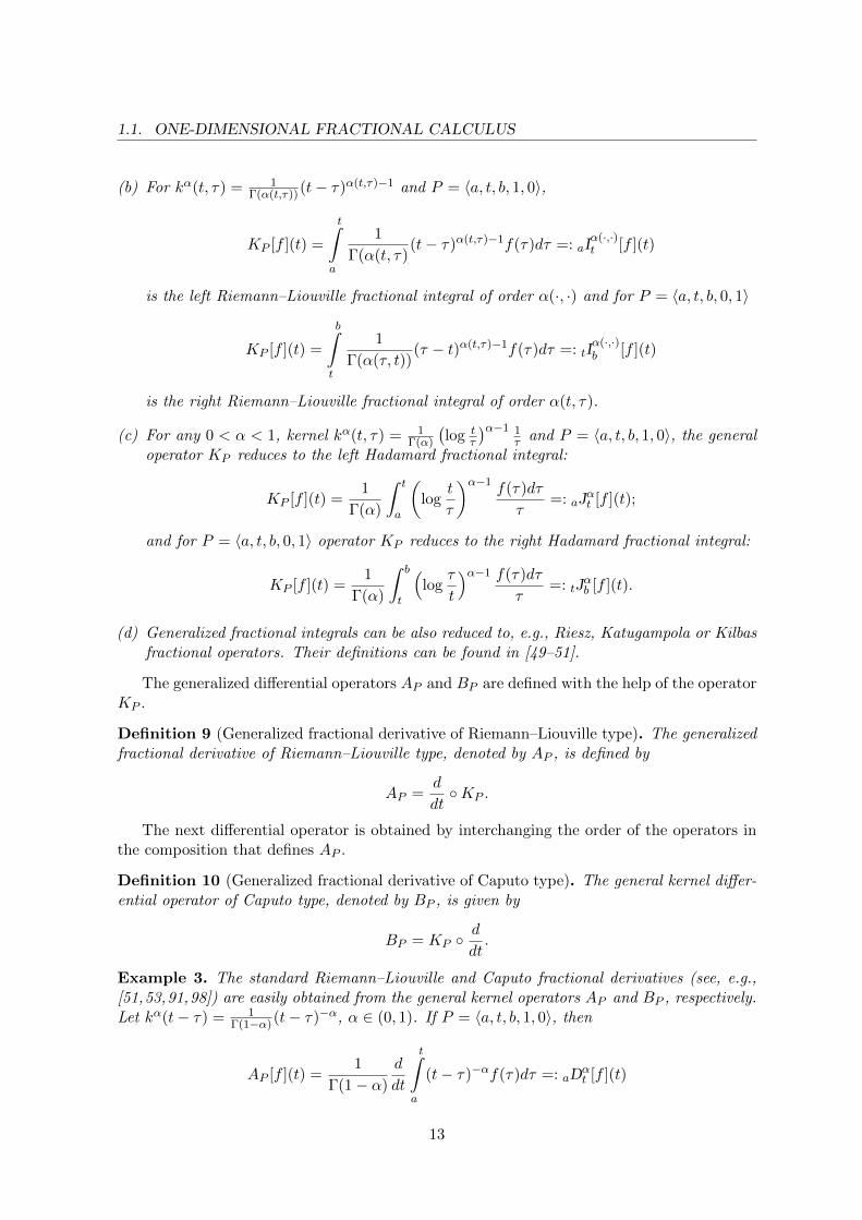
1.1. ONE-DIMENSIONAL FRACTIONAL CALCULUS
(b) For kα(t, τ) = 1Γ(α(t,τ))(t− τ)α(t,τ)−1 and P = 〈a, t, b, 1, 0〉,
KP [f ](t) =
t∫a
1
Γ(α(t, τ)(t− τ)α(t,τ)−1f(τ)dτ =: aI
α(·,·)t [f ](t)
is the left Riemann–Liouville fractional integral of order α(·, ·) and for P = 〈a, t, b, 0, 1〉
KP [f ](t) =
b∫t
1
Γ(α(τ, t))(τ − t)α(t,τ)−1f(τ)dτ =: tI
α(·,·)b [f ](t)
is the right Riemann–Liouville fractional integral of order α(t, τ).
(c) For any 0 < α < 1, kernel kα(t, τ) = 1Γ(α)
(log t
τ
)α−1 1τ and P = 〈a, t, b, 1, 0〉, the general
operator KP reduces to the left Hadamard fractional integral:
KP [f ](t) =1
Γ(α)
∫ t
a
(log
t
τ
)α−1 f(τ)dτ
τ=: aJ
αt [f ](t);
and for P = 〈a, t, b, 0, 1〉 operator KP reduces to the right Hadamard fractional integral:
KP [f ](t) =1
Γ(α)
∫ b
t
(log
τ
t
)α−1 f(τ)dτ
τ=: tJ
αb [f ](t).
(d) Generalized fractional integrals can be also reduced to, e.g., Riesz, Katugampola or Kilbasfractional operators. Their definitions can be found in [49–51].
The generalized differential operators AP and BP are defined with the help of the operatorKP .
Definition 9 (Generalized fractional derivative of Riemann–Liouville type). The generalizedfractional derivative of Riemann–Liouville type, denoted by AP , is defined by
AP =d
dtKP .
The next differential operator is obtained by interchanging the order of the operators inthe composition that defines AP .
Definition 10 (Generalized fractional derivative of Caputo type). The general kernel differ-ential operator of Caputo type, denoted by BP , is given by
BP = KP d
dt.
Example 3. The standard Riemann–Liouville and Caputo fractional derivatives (see, e.g.,[51,53,91,98]) are easily obtained from the general kernel operators AP and BP , respectively.Let kα(t− τ) = 1
Γ(1−α)(t− τ)−α, α ∈ (0, 1). If P = 〈a, t, b, 1, 0〉, then
AP [f ](t) =1
Γ(1− α)
d
dt
t∫a
(t− τ)−αf(τ)dτ =: aDαt [f ](t)
13

CHAPTER 1. FRACTIONAL CALCULUS
is the standard left Riemann–Liouville fractional derivative of order α, while
BP [f ](t) =1
Γ(1− α)
t∫a
(t− τ)−αf ′(τ)dτ =: Ca Dαt [f ](t)
is the standard left Caputo fractional derivative of order α; if P = 〈a, t, b, 0, 1〉, then
−AP [f ](t) = − 1
Γ(1− α)
d
dt
b∫t
(τ − t)−αf(τ)dτ =: tDαb [f ](t)
is the standard right Riemann–Liouville fractional derivative of order α, while
−BP [f ](t) = − 1
Γ(1− α)
b∫t
(τ − t)−αf ′(τ)dτ =: Ct Dαb [f ](t)
is the standard right Caputo fractional derivative of order α.
1.2 Multidimensional Fractional Calculus
In this section, we introduce notions of classical, variable order and generalized partialfractional integrals and derivatives, in a multidimensional finite domain. They are natu-ral generalizations of the corresponding fractional operators of Section 1.1.1. Furthermore,similarly as in the integer order case, computation of partial fractional derivatives and inte-grals is reduced to the computation of one-variable fractional operators. Along the work, fori = 1, . . . , n, let ai, bi and αi be numbers in R and t = (t1, . . . , tn) be such that t ∈ Ωn, whereΩn = (a1, b1)× · · · × (an, bn) is a subset of Rn. Moreover, let us define the following sets:
∆i :=
(ti, τ) ∈ R2 : ai ≤ τ < ti ≤ bi, i = 1 . . . , n.
1.2.1 Classical Partial Fractional Integrals and Derivatives
In this section we present definitions of classical partial fractional integrals and derivatives.Interested reader can find more details in Section 24.1 of the book [98].
Definition 11 (Left and right Riemann–Liouville partial fractional integrals). Let t ∈ Ωn.The left and the right partial Riemann–Liouville fractional integrals of order αi ∈ R (αi > 0)with respect to the ith variable ti are defined by
aiIαiti
[f ](t) :=1
Γ(αi)
∫ ti
ai
f(t1, . . . , ti−1, τ, ti+1, . . . , tn)dτ
(ti − τ)1−αi, ti > ai, (1.13)
and
tiIαibi
[f ](t) :=1
Γ(αi)
∫ bi
ti
f(t1, . . . , ti−1, τ, ti+1, . . . , tn)dτ
(τ − ti)1−α , ti < bi, (1.14)
respectively.
14
1.2. MULTIDIMENSIONAL FRACTIONAL CALCULUS
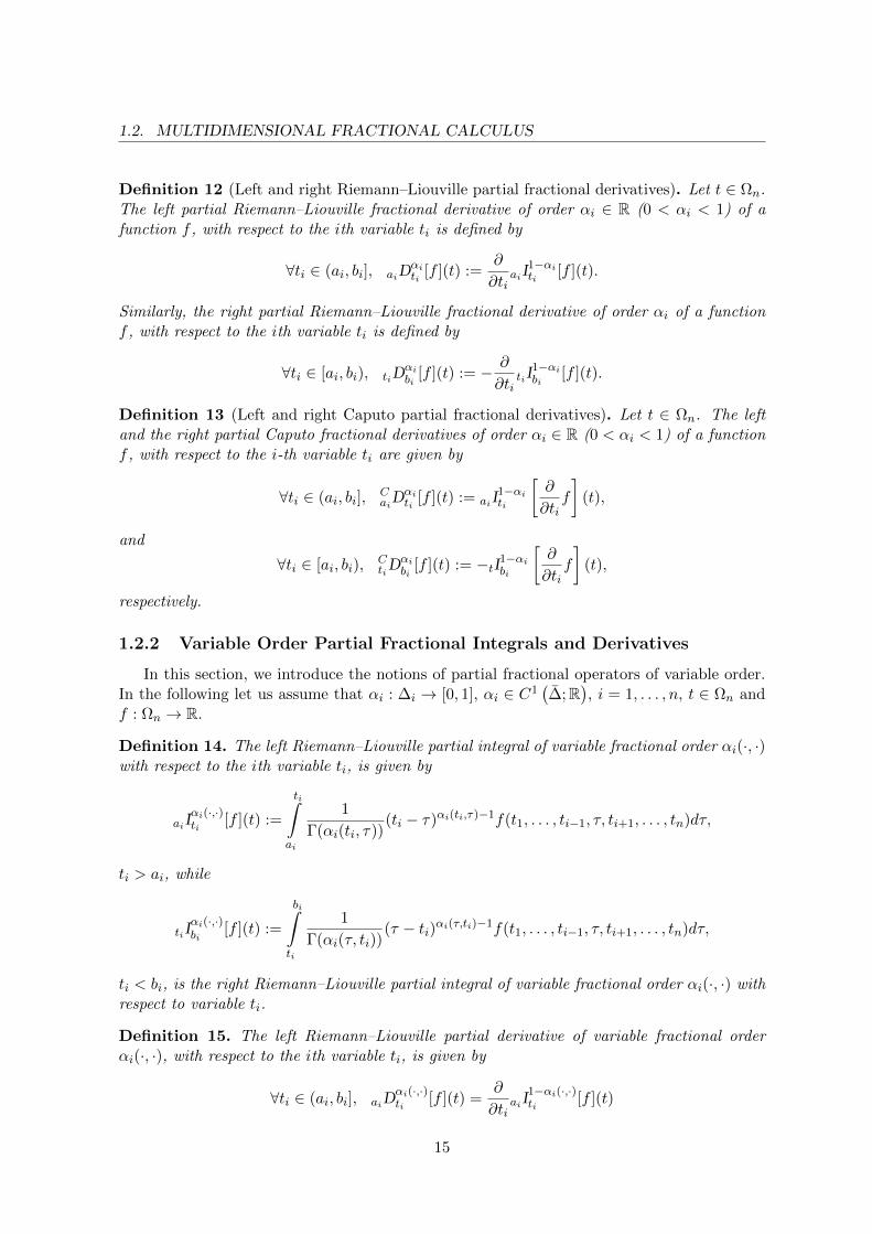
Definition 12 (Left and right Riemann–Liouville partial fractional derivatives). Let t ∈ Ωn.The left partial Riemann–Liouville fractional derivative of order αi ∈ R (0 < αi < 1) of afunction f , with respect to the ith variable ti is defined by
∀ti ∈ (ai, bi], aiDαiti
[f ](t) :=∂
∂tiaiI
1−αiti
[f ](t).
Similarly, the right partial Riemann–Liouville fractional derivative of order αi of a functionf , with respect to the ith variable ti is defined by
∀ti ∈ [ai, bi), tiDαibi
[f ](t) := − ∂
∂titiI
1−αibi
[f ](t).
Definition 13 (Left and right Caputo partial fractional derivatives). Let t ∈ Ωn. The leftand the right partial Caputo fractional derivatives of order αi ∈ R (0 < αi < 1) of a functionf , with respect to the i-th variable ti are given by
∀ti ∈ (ai, bi],CaiD
αiti
[f ](t) := aiI1−αiti
[∂
∂tif
](t),
and
∀ti ∈ [ai, bi),CtiD
αibi
[f ](t) := −tI1−αibi
[∂
∂tif
](t),
respectively.
1.2.2 Variable Order Partial Fractional Integrals and Derivatives
In this section, we introduce the notions of partial fractional operators of variable order.In the following let us assume that αi : ∆i → [0, 1], αi ∈ C1
(∆;R
), i = 1, . . . , n, t ∈ Ωn and
f : Ωn → R.
Definition 14. The left Riemann–Liouville partial integral of variable fractional order αi(·, ·)with respect to the ith variable ti, is given by
aiIαi(·,·)ti
[f ](t) :=
ti∫ai
1
Γ(αi(ti, τ))(ti − τ)αi(ti,τ)−1f(t1, . . . , ti−1, τ, ti+1, . . . , tn)dτ,
ti > ai, while
tiIαi(·,·)bi
[f ](t) :=
bi∫ti
1
Γ(αi(τ, ti))(τ − ti)αi(τ,ti)−1f(t1, . . . , ti−1, τ, ti+1, . . . , tn)dτ,
ti < bi, is the right Riemann–Liouville partial integral of variable fractional order αi(·, ·) withrespect to variable ti.
Definition 15. The left Riemann–Liouville partial derivative of variable fractional orderαi(·, ·), with respect to the ith variable ti, is given by
∀ti ∈ (ai, bi], aiDαi(·,·)ti
[f ](t) =∂
∂tiaiI
1−αi(·,·)ti
[f ](t)
15

CHAPTER 1. FRACTIONAL CALCULUS
while the right Riemann–Liouville partial derivative of variable fractional order αi(·, ·), withrespect to the ith variable ti, is defined by
∀ti ∈ [ai, bi), tiDαi(·,·)bi
[f ](t) = − ∂
∂titiI
1−αi(·,·)bi
[f ](t)
Definition 16. The left Caputo partial derivative of variable fractional order αi(·, ·), withrespect to the ith variable ti, is defined by
∀ti ∈ (ai, bi],CaiD
αi(·,·)ti
[f ](t) = aiI1−αi(·,·)ti
[∂
∂tif
](t),
while the right Caputo partial derivative of variable fractional order αi(·, ·), with respect tothe ith variable ti, is given by
∀ti ∈ [ai, bi),CtiD
αi(·,·)bi
[f ](t) = −tiI1−αi(·,·)bi
[∂
∂tif
](t).
Note that, if αi(·, ·) is a constant function, then the partial operators of variable frac-tional order are reduced to corresponding partial integrals and derivatives of constant orderintroduced in Section 1.2.1.
1.2.3 Generalized Partial Fractional Operators
Let us assume that λ = (λ1, . . . , λn) and µ = (µ1, . . . , µn) are in Rn. We shall presentdefinitions of generalized partial fractional integrals and derivatives. Let ki : ∆i → R, i =1 . . . , n and t ∈ Ωn.
Definition 17 (Generalized partial fractional integral). For any function f defined almosteverywhere on Ωn with value in R, the generalized partial integral KPi is defined for almostall ti ∈ (ai, bi) by:
KPi [f ](t) := λi
ti∫ai
ki(ti, τ)f(t1, . . . , ti−1, τ, ti+1, . . . , tn)dτ
+ µi
bi∫ti
ki(τ, ti)f(t1, . . . , ti−1, τ, ti+1, . . . , tn)dτ,
where Pi = 〈ai, ti, bi, λi, µi〉.
Definition 18 (Generalized partial fractional derivative of Riemann–Liouville type). Thegeneralized partial fractional derivative of Riemann–Liouville type with respect to the ith vari-able ti is given by
APi :=∂
∂tiKPi .
Definition 19 (Generalized partial fractional derivative of Caputo type). The generalizedpartial fractional derivative of Caputo type with respect to the ith variable ti is given by
BPi := KPi ∂
∂ti.
16
1.2. MULTIDIMENSIONAL FRACTIONAL CALCULUS
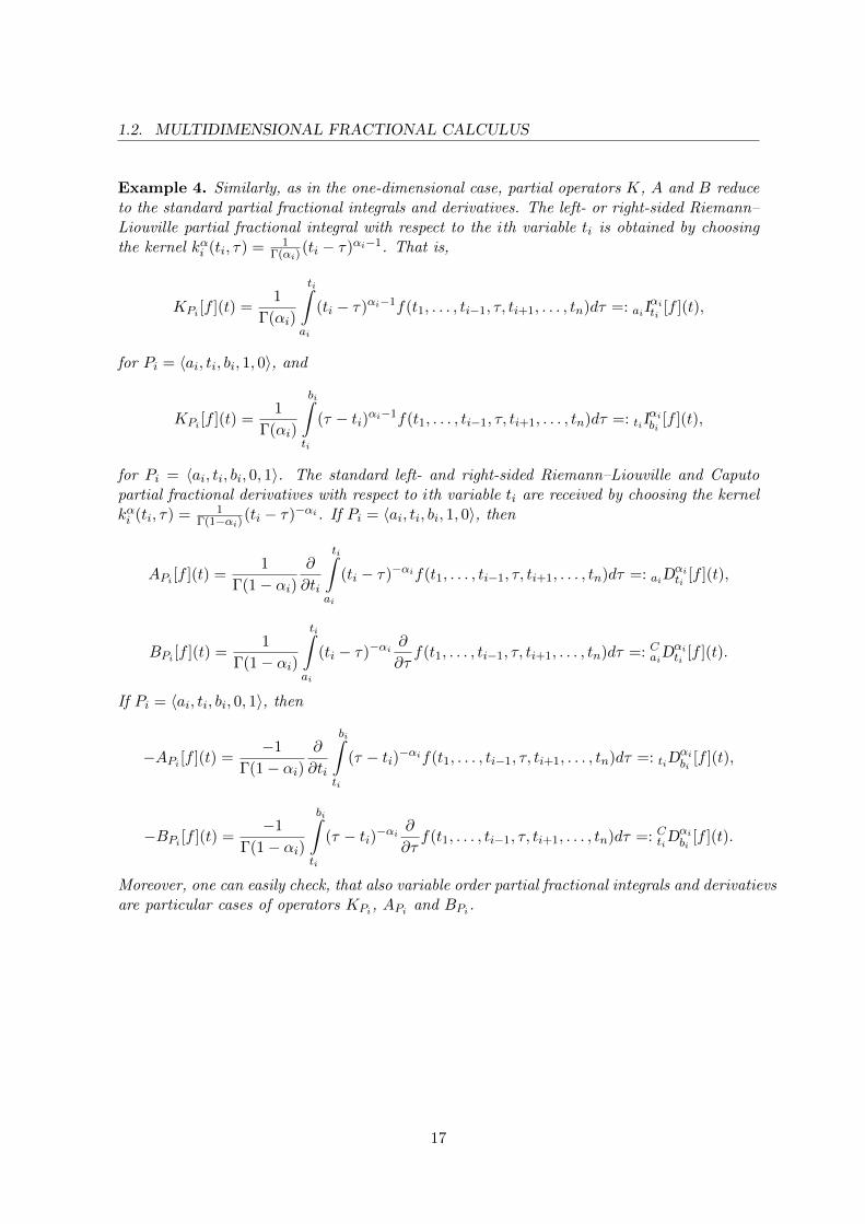
Example 4. Similarly, as in the one-dimensional case, partial operators K, A and B reduceto the standard partial fractional integrals and derivatives. The left- or right-sided Riemann–Liouville partial fractional integral with respect to the ith variable ti is obtained by choosingthe kernel kαi (ti, τ) = 1
Γ(αi)(ti − τ)αi−1. That is,
KPi [f ](t) =1
Γ(αi)
ti∫ai
(ti − τ)αi−1f(t1, . . . , ti−1, τ, ti+1, . . . , tn)dτ =: aiIαiti
[f ](t),
for Pi = 〈ai, ti, bi, 1, 0〉, and
KPi [f ](t) =1
Γ(αi)
bi∫ti
(τ − ti)αi−1f(t1, . . . , ti−1, τ, ti+1, . . . , tn)dτ =: tiIαibi
[f ](t),
for Pi = 〈ai, ti, bi, 0, 1〉. The standard left- and right-sided Riemann–Liouville and Caputopartial fractional derivatives with respect to ith variable ti are received by choosing the kernelkαi (ti, τ) = 1
Γ(1−αi)(ti − τ)−αi. If Pi = 〈ai, ti, bi, 1, 0〉, then
APi [f ](t) =1
Γ(1− αi)∂
∂ti
ti∫ai
(ti − τ)−αif(t1, . . . , ti−1, τ, ti+1, . . . , tn)dτ =: aiDαiti
[f ](t),
BPi [f ](t) =1
Γ(1− αi)
ti∫ai
(ti − τ)−αi∂
∂τf(t1, . . . , ti−1, τ, ti+1, . . . , tn)dτ =: CaiD
αiti
[f ](t).
If Pi = 〈ai, ti, bi, 0, 1〉, then
−APi [f ](t) =−1
Γ(1− αi)∂
∂ti
bi∫ti
(τ − ti)−αif(t1, . . . , ti−1, τ, ti+1, . . . , tn)dτ =: tiDαibi
[f ](t),
−BPi [f ](t) =−1
Γ(1− αi)
bi∫ti
(τ − ti)−αi∂
∂τf(t1, . . . , ti−1, τ, ti+1, . . . , tn)dτ =: CtiD
αibi
[f ](t).
Moreover, one can easily check, that also variable order partial fractional integrals and derivatievsare particular cases of operators KPi, APi and BPi.
17

Chapter 2
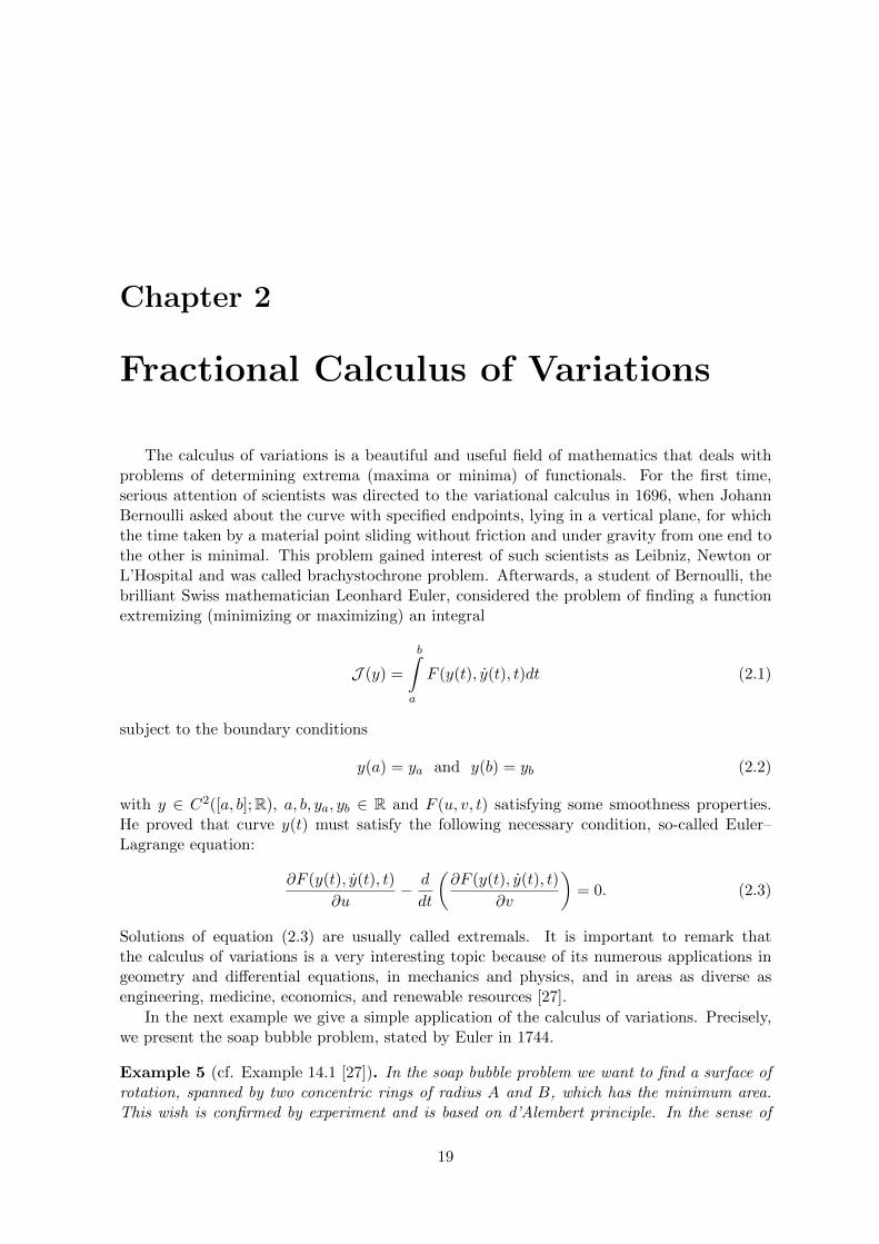
Fractional Calculus of Variations
The calculus of variations is a beautiful and useful field of mathematics that deals withproblems of determining extrema (maxima or minima) of functionals. For the first time,serious attention of scientists was directed to the variational calculus in 1696, when JohannBernoulli asked about the curve with specified endpoints, lying in a vertical plane, for whichthe time taken by a material point sliding without friction and under gravity from one end tothe other is minimal. This problem gained interest of such scientists as Leibniz, Newton orL’Hospital and was called brachystochrone problem. Afterwards, a student of Bernoulli, thebrilliant Swiss mathematician Leonhard Euler, considered the problem of finding a functionextremizing (minimizing or maximizing) an integral
J (y) =
b∫a
F (y(t), y(t), t)dt (2.1)
subject to the boundary conditions
y(a) = ya and y(b) = yb (2.2)
with y ∈ C2([a, b];R), a, b, ya, yb ∈ R and F (u, v, t) satisfying some smoothness properties.He proved that curve y(t) must satisfy the following necessary condition, so-called Euler–Lagrange equation:
∂F (y(t), y(t), t)
∂u− d
dt
(∂F (y(t), y(t), t)
∂v
)= 0. (2.3)
Solutions of equation (2.3) are usually called extremals. It is important to remark thatthe calculus of variations is a very interesting topic because of its numerous applications ingeometry and differential equations, in mechanics and physics, and in areas as diverse asengineering, medicine, economics, and renewable resources [27].
In the next example we give a simple application of the calculus of variations. Precisely,we present the soap bubble problem, stated by Euler in 1744.
Example 5 (cf. Example 14.1 [27]). In the soap bubble problem we want to find a surface ofrotation, spanned by two concentric rings of radius A and B, which has the minimum area.This wish is confirmed by experiment and is based on d’Alembert principle. In the sense of
19
CHAPTER 2. FRACTIONAL CALCULUS OF VARIATIONS
the calculus of variations, we can formulate the soap bubble problem in the following way: wewant to minimize the variational functional
J (y) =
b∫a
y(t)√
1 + y(t)2dt subject to y(a) = A, y(b) = B.
This is a special case of problem (2.1)-(2.2) with F (u, v, t) = u√
1 + v2. Let y(t) > 0 ∀t. It isnot difficult to verify that the Euler–Lagrange equation is given by
y(t) =1 + y(t)2
y(t)
and its solution is the catenary curve given by
y(t) = k cosh
(t+ c
k
),
where c, k are certain constants.
This thesis is devoted to the fractional calculus of variations and its generalizations. There-fore in the next sections we present basic results of the non-integer variational calculus. Letus precise, that along the work we will understand ∂iF as the partial derivative of functionF with respect to its ith argument.
2.1 Fractional Euler–Lagrange Equations
Within the years, several methods were proposed to solve mechanical problems with non-conservative forces, e.g., Rayleigh dissipation function method, technique introducing an aux-iliary coordinate or approach including the microscopic details of the dissipation directly inthe Lagrangian. Although, all mentioned methods are correct, they are not as direct andsimple as it is in the case of conservative systems. In the notes from 1996-1997, Riewe pre-sented a new approach to nonconservative forces [96, 97]. He claimed that friction forcesfollow from Lagrangians containing terms proportional to fractional derivatives. Precisely,for y : [a, b]→ Rr and αi, βj ∈ [0, 1], i = 1, . . . , N , j = 1, . . . , N ′, he considered the followingenergy functional:
J (y) =
b∫a
F(aD
α1t [y](t), . . . ,aD
αNt [y](t),tD
β1b [y](t), . . . ,tD
βN′b [y](t), y(t), t
)dt,
with r, N and N ′ being natural numbers. Using the fractional variational principle he ob-tained the following Euler–Lagrange equation:
N∑i=1
tDαib [∂iF ] +
N ′∑i=1
aDβit [∂i+NF ] + ∂N ′+N+1F = 0. (2.4)
Riewe illustrated his results through the classical problem of linear friction.
20

2.1. FRACTIONAL EULER–LAGRANGE EQUATIONS
Example 6 ( [97]). Let us consider the following Lagrangian:
F =1
2my2 − V (y) +
1
2γi
(aD
12t [y]
)2
, (2.5)
where the first term in the sum represents kinetic energy, the second one potential energy, thelast one is linear friction energy and i2 = −1. Using (2.4) we can obtain the Euler–Lagrangeequation for a Lagrangian containing derivatives of order one and order 1
2 :
∂F
∂y+ tD
12b
∂F
∂aD12t [y]
− d
dt
∂F
∂y= 0,
which, in the case of Lagrangian (2.5), becomes
my = −γi(tD
12b aD
12t
)[y]− ∂V (y)
∂y.
In order to obtain the equation with linear friction, my + γy + ∂V∂y = 0, Riewe suggested
considering an infinitesimal time interval, that is, the limiting case a → b, while keepinga < b.
After the works of Riewe several authors contributed to the theory of the fractional vari-ational calculus. First, let us point out the approach discussed by Klimek in [52]. It wassuggested to study symmetric fractional derivatives of order α (0 < α < 1) defined as follows:
Dα :=1
2aD
αt +
1
2tD
αb .
In contrast to the left and right fractional derivatives, operator Dα is symmetric for the scalarproduct given by
〈f |g〉 :=
b∫a
f(t)g(t) dt,
that is,
〈Dα[f ]|g〉 = 〈f |Dα[g]〉.
With this notion for the fractional derivative, for αi ∈ (0, 1) and y : [a, b]→ Rr, i = 1, . . . , N ,Klimek considered the following action functional:
J (y) =
b∫a
F (Dα1 [y](t), . . . ,DαN [y](t), y(t), t) dt. (2.6)
Using the fractional variational principle, she derived the Euler–Lagrange equation given by
∂N+1F +N∑i=1
Dαi [∂iF ] = 0. (2.7)
21
CHAPTER 2. FRACTIONAL CALCULUS OF VARIATIONS
As an example Klimek considered the following variational functional
J (y) =
b∫a
2my2(t)− γi(D
12 [y](t)
)2− V (y(t)) dt
and under appropriate assumptions arrived to the equation with linear friction
my = −∂V∂y− γy. (2.8)
Another type of problems, containing Riemann–Liouville fractional derivatives, was dis-cussed by Klimek in [53]:
J (y) =
b∫a
F (aDα1t [y](t), . . . ,aD
αNt [y](t), y(t), t)dt
and the Euler–Lagrange equation
∂N+1F +
N∑i=1
Ct D
αib [∂iF ] = 0 (2.9)
including fractional derivatives of the Caputo type was obtained.The next examples are borrowed from [53].
Example 7 (cf. Example 4.1.1 of [53]). Let 0 < α < 1 and y be a minimizer of the functional
J (y) =
b∫a
1
2y(t)aD
αt [y](t)dt.
Then y is a solution to the following Euler–Lagrange equation:
1
2
(aD
αt [y] + C
t Dαb [y]
)= 0.
Example 8 (cf. Example 4.1.2 of [53]). Let 0 < α < 1. The model of harmonic oscillator,in the framework of classical mechanics, is connected to an action
J (y) =
b∫a
[−1
2y′2(t) +
ω2
2y2(t)
]dt, (2.10)
and is determined by the following equation
y′′ + ω2y = 0. (2.11)
If in functional (2.10) instead of derivative of order one we put a derivative of fractional orderα, then
J (y) =
b∫a
[−1
2(aD
αt [y](t))2 +
ω2
2y2(t)
]dt,
and by (2.9) the Euler–Lagrange equation has the following form:
−Ct Dαb [aD
αt [y]] + ω2y = 0. (2.12)
If α→ 1+, then equation (2.12) reduces to (2.11). The proof of this fact, as well as solutionsto fractional harmonic oscillator equation (2.12), can be found in [53].
22

2.2. FRACTIONAL EMBEDDING OF EULER–LAGRANGE EQUATIONS
2.2 Fractional Embedding of Euler–Lagrange Equations
The notion of embedding introduced in [30] is an algebraic procedure providing an ex-tension of classical differential equations over an arbitrary vector space. This formalism isdeveloped in the framework of stochastic processes [30], non-differentiable functions [31], andfractional equations [29]. The general scheme of embedding theories is the following: (i) fixa vector space V and a mapping ι : C0([a, b],Rn)→ V ; (ii) extend differential operators overV ; (iii) extend the notion of integral over V . Let (ι,D, J) be a given embedding formalism,where a linear operator D : V → V takes place for a generalized derivative on V , and alinear operator J : V → R takes place for a generalized integral on V . The embedding pro-cedure gives two different ways, a priori, to generalize Euler–Lagrange equations. The first(pure algebraic) way is to make a direct embedding of the Euler–Lagrange equation. Thesecond (analytic) is to embed the Lagrangian functional associated to the equation and to de-rive, by the associated calculus of variations, the Euler–Lagrange equation for the embeddedfunctional. A natural question is then the problem of coherence between these two extensions:
Coherence problem. Let (ι,D, J) be a given embedding formalism. Do we have equiv-alence between the Euler–Lagrange equation which gives the direct embedding and the onereceived from the embedded Lagrangian system?
As shown in the work [29] for standard fractional differential calculus, the answer to thequestion above is known to be negative. To be more precise, let us define the followingoperator first introduced in [29].
Definition 20 (Fractional operator of order (α, β)). Let a, b ∈ R, a < b and µ ∈ C. Wedefine the fractional operator of order (α, β), with α > 0 and β > 0, by
Dα,βµ =1
2
[aD
αt −t D
βb
]+iµ
2
[aD
αt +t D
βb
]. (2.13)
In particular, for α = β = 1 one has D1,1µ = d
dt . Moreover, for µ = −i we recover the leftRiemann–Liouville fractional derivative of order α,
Dα,β−i = aDαt ,
and for µ = i the right Riemann–Liouville fractional derivative of order β:
Dα,βi = −tDαb .
Now, let us consider the following variational functional:
J (y) =
b∫a
F (Dα,βµ [y](t), y(t), t)dt
defined on the space of continuous functions such that aDαt [y] together with tD
βb [y] exist and
y(a) = ya, y(b) = yb. Using the direct embedding procedure, the Euler–Lagrange equationderived by Cresson is
Dβ,α−µ [∂1F ] = ∂2F. (2.14)
Using the variational principle in derivation of the Euler–Lagrange equation, one has
Dα,βµ [∂1F ] = ∂2F. (2.15)
23

CHAPTER 2. FRACTIONAL CALCULUS OF VARIATIONS
Reader can easily notice that, in general, there is a difference between equations (2.14) and(2.15) i.e., they are not coherent. Cresson claimed [29] that this lack of coherence has thefollowing sources:
• the set of variations in the method of variational principle is to large and thereforeit does not give correct answer; one should find the corresponding constraints for thevariations;
• there is a relation between lack of coherence and properties of the operator used togeneralize the classical derivative.
Let us observe that coherence between (2.14) and (2.15) is restored in the case when α = βand µ = 0. This type of coherence is called time reversible coherence . For a deeper discussionof the subject we refer the reader to [29].
In this chapter we presented few results of the fractional calculus of variations. A com-prehensive study of the subject can be found in the books [53,70].
24
Part II
Original Work
25


Chapter 3
Standard Methods in FractionalVariational Calculus
The model problem of this chapter is to find an admissible function giving a minimumvalue to the integral functional, which depends on an unknown function (or functions) of oneor several variables and its generalized fractional derivatives and/or generalized fractionalintegrals. In order to answer this question, we will make use of the standard methods in thefractional calculus of variations (see e.g., [70]). Namely, by analogy to the classical variationalcalculus (see e.g., [33]), the approach that we call standard, is first to prove Euler–Lagrangeequations, find their solutions and then to check if they are minimizers. It is important toremark that standard methods suffer an important disadvantage. Precisely, solvability ofEuler–Lagrange equations is assumed, which is not the case in direct methods that are goingto be presented later (see Chapter 4).
Now, before we describe briefly an arrangement of this chapter, we define the concept ofminimizer. Let (X, ‖·‖) be normed linear space and I be a functional defined on a nonemptysubset A of X. Moreover, let us introduce the following set: if y ∈ A and δ > 0, then
Nδ(y) := y ∈ A : ‖y − y‖ < δ
is called neighborhood of y in A.
Definition 21. Function y ∈ A is called minimizer of I if there exists a neighborhood Nδ(y)of y such that
I(y) ≤ I(y), for all y ∈ Nδ(y).
Note that any function y ∈ Nδ(y) can be represented in a convenient way as a perturbationof y. Precisely,
∀y ∈ Nδ(y), ∃η ∈ A0, y = y + hη, |h| ≤ ε,
where 0 < ε < δ‖η‖ and A0 is a suitable set of functions η such that
A0 = η ∈ X : y + hη ∈ A, |h| ≤ ε .
We begin the chapter with Section 3.1, where we prove generalized integration by partsformula and boundedness of generalized fractional integral from Lp(a, b;R)to Lq(a, b;R).
In Section 3.2 we consider the one-dimensional fundamental problem with generalizedfractional operators and obtain an appropriate Euler–Lagrange equation. Then, we prove
27

CHAPTER 3. STANDARD METHODS IN FRACTIONAL VARIATIONAL CALCULUS
that under some convexity assumptions on Lagrangian, every solution to the Euler–Lagrangeequation is automatically a solution to our problem. Moreover, as corollaries, we obtainresults for problems of the constant and variable order fractional variational calculus anddiscuss some illustrative examples.
In Section 3.3 we study variational problems with free end points and besides Euler–Lagrange equations we prove natural boundary conditions. As particular cases we obtainnatural boundary conditions for problems with constant and variable order fractional opera-tors.
Section 3.4 is devoted to generalized fractional isoperimetric problems. We want to findfunctions that minimize an integral functional subject to given boundary conditions andisoperimetric constraints. We prove necessary optimality conditions and, as corollaries, weobtain Euler–Lagrange equations for isoperimetric problems with constant and variable orderfractional operators. Furthermore, we illustrate our results through several examples.
In Section 3.5 we prove a generalized fractional counterpart of Noether’s theorem. Assum-ing invariance of the functional, we prove that any extremal must satisfy a certain generalizedfractional equation. Corresponding results are obtained for functionals with constant andvariable order fractional operators.
Section 3.6 is dedicated to variational problems defined by the use of the generalizedfractional integral instead of the classical integral. We obtain Euler–Lagrange equations anddiscuss several examples.
Finally, in Section 3.7 we study multidimensional fractional variational problems withgeneralized partial operators. We begin with the proofs of integration by parts formulas forgeneralized partial fractional integrals and derivatives. Next, we use these results to showEuler–Lagrange equations for the fundamental problem. Moreover, we prove a generalizedfractional Dirichlet’s principle, necessary optimality condition for the isoperimetric problemand Noether’s theorem. We finish the chapter with some conclusions.
3.1 Properties of Generalized Fractional Integrals
This section is devoted to properties of generalized fractional operators. We begin byproving in Section 3.1.1 that the generalized fractional operator KP is bounded and linear.Later, in Section 3.1.2, we give integration by parts formulas for generalized fractional oper-ators.
3.1.1 Boundedness of Generalized Fractional Operators
Along the work, we assume that 1 < p <∞ and that q is an adjoint of p, that is 1p + 1
q = 1.Let us prove the following theorem yielding boundedness of the generalized fractional integralKP from Lp(a, b;R) to Lq(a, b;R).
Theorem 1. Let us assume that k ∈ Lq(∆;R). Then, KP is a linear bounded operator fromLp(a, b;R) to Lq(a, b;R).
Proof. The linearity is obvious. We will show that KP is bounded from Lp(a, b;R) toLq(a, b;R). Considering only the first term of KP , let us prove that the following inequality
28

3.1. PROPERTIES OF GENERALIZED FRACTIONAL INTEGRALS
holds for any f ∈ Lp(a, b;R): b∫a
∣∣∣∣∣∣t∫
a
k(t, τ)f(τ) dτ
∣∣∣∣∣∣q
dt
1/q
≤ ‖k‖Lq(∆,R) ‖f‖Lp . (3.1)
Using Fubini’s theorem, we have k(t, ·) ∈ Lq(a, t;R) for almost all t ∈ (a, b). Then, applyingHolder’s inequality, we have∣∣∣∣∣∣
t∫a
k(t, τ)f(τ) dτ
∣∣∣∣∣∣q
≤
t∫a
|k(t, τ)|q dτ
1q t∫a
|f(τ)|p dτ
1p
q
≤t∫
a
|k(t, τ)|q dτ ‖f‖qLp
(3.2)for almost all t ∈ (a, b). Hence, integrating equation (3.2) on the interval (a, b), we obtaininequality (3.1). The proof is completed using the same strategy on the second term in thedefinition of KP .
Corollary 1. If 1p < α < 1, then aI
αt is a linear bounded operator from Lp(a, b;R) to
Lq(a, b;R).
Proof. Let us denote kα(t, τ) = 1Γ(α)(t− τ)α−1. For 1
p < α < 1 there exist a constant C ∈ Rsuch that for almost all t ∈ (a, b)
t∫a
|kα(t, τ)|q dτ ≤ C. (3.3)
Integrating (3.3) on the (a, b) we have kα(t, τ) ∈ Lq(∆;R). Therefore, applying Theorem 1with P = 〈a, t, b, 1, 0〉 operator aI
αt is linear bounded from Lp(a, b;R) to Lq(a, b;R).
Next result shows that with the use of Theorem 1, one can prove that variable orderfractional integral is a linear bounded operator.
Corollary 2. Let α : ∆ → [δ, 1] with δ > 1p . Then aI
α(·,·)t is linear bounded operator from
Lp(a, b;R) to Lq(a, b;R).
Proof. Let us denote kα(t, τ) = (t − τ)α(t,τ)−1/Γ(α(t, τ)). We have just to prove that kα ∈Lq(∆,R) in order to use Theorem 1. Let us note that since α is with values in [δ, 1] withδ > 0, then 1/(Γ α) is bounded. Hence, we have just to prove that (Γ α)kα ∈ Lq(∆,R).We have two different cases: b− a ≤ 1 and b− a > 1.
In the first case, for any (t, τ) ∈ ∆, we have 0 < t− τ ≤ 1 and q(δ − 1) > −1. Then:
t∫a
(t− τ)q(α(t,τ)−1) dτ ≤t∫
a
(t− τ)q(δ−1) dτ =(t− a)q(δ−1)+1
q(δ − 1) + 1≤ 1
q(δ − 1) + 1.
In the second case, for almost all (t, τ) ∈ ∆ ∩ (a, a + 1) × (a, b), we have 0 < t − τ ≤ 1.Consequently, we conclude in the same way that:
t∫a
(t− τ)q(α(t,τ)−1) dτ ≤ 1
q(δ − 1) + 1.
29
CHAPTER 3. STANDARD METHODS IN FRACTIONAL VARIATIONAL CALCULUS
Still in the second case, for almost all (t, τ) ∈ ∆ ∩ (a + 1, b) × (a, b), we have τ < t − 1 ort− 1 ≤ τ ≤ t. Then:
t∫a
(t−τ)q(α(t,τ)−1) dτ =
t−1∫a
(t−τ)q(α(t,τ)−1) dτ+
t∫t−1
(t−τ)q(α(t,τ)−1) dτ ≤ b−a−1+1
q(δ − 1) + 1.
Consequently, in any case, there exist a constant C ∈ R such that for almost all t ∈ (a, b):
t∫a
|kα(t, τ)|q dτ ≤ C. (3.4)
Finally, kα ∈ Lq(∆,R).
3.1.2 Generalized Fractional Integration by Parts
In this section we obtain formula of integration by parts for the generalized fractionalcalculus. Our results are particularly useful with respect to applications in dynamic opti-mization, where the derivation of the Euler–Lagrange equations uses, as a key step in theproof, integration by parts (see e.g., the proof of Theorem 3 in Section 3.2).
In our setting, integration by parts changes a given parameter set P into its dual P ∗. Theterm duality comes from the fact that P ∗∗ = P .
Definition 22 (Dual parameter set). Given a parameter set P = 〈a, t, b, λ, µ〉 we denote byP ∗ the parameter set P ∗ = 〈a, t, b, µ, λ〉. We say that P ∗ is the dual of P .
Our first formula of fractional integration by parts involves the operator KP .
Theorem 2. Let us assume that k ∈ Lq(∆;R). Then, the operator KP ∗ defined by
KP ∗ [f ](t) = µ
t∫a
k(t, τ)f(τ) dτ + λ
b∫t
k(τ, t)f(τ) dτ (3.5)
is a linear bounded operator from Lp(a, b;R) to Lq(a, b;R). Moreover, the following integrationby parts formula holds:
b∫a
f(t) ·KP [g](t) dt =
b∫a
g(t) ·KP ∗ [f ](t) dt, (3.6)
for any f, g ∈ Lp(a, b;R).
Proof. Using Theorem 1, we obtain that KP ∗ is a linear bounded operator from Lp(a, b;R)to Lq(a, b;R). The second part is easily proved using Fubini’s theorem. Indeed, consideringonly the first term of KP , the following equality holds for any f, g ∈ Lp(a, b;R):
λ
b∫a
f(t) ·t∫
a
k(t, τ)g(τ) dτ dt = λ
b∫a
g(τ) ·b∫τ
k(t, τ)f(t) dt dτ.
The proof is completed by using the same strategy on the second part of the definition ofKP .
30
3.1. PROPERTIES OF GENERALIZED FRACTIONAL INTEGRALS
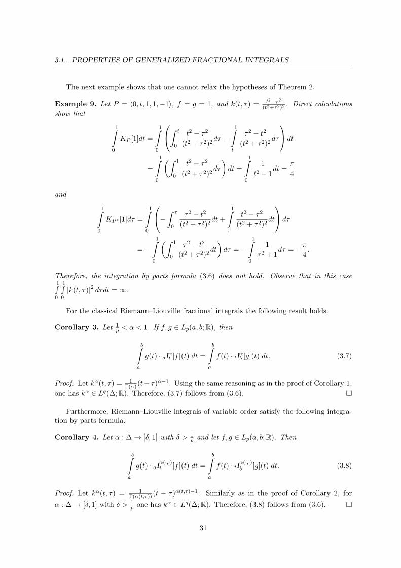
The next example shows that one cannot relax the hypotheses of Theorem 2.
Example 9. Let P = 〈0, t, 1, 1,−1〉, f = g = 1, and k(t, τ) = t2−τ2(t2+τ2)2
. Direct calculations
show that
1∫0
KP [1]dt =
1∫0
∫ t
0
t2 − τ2
(t2 + τ2)2dτ −
1∫t
τ2 − t2
(t2 + τ2)2dτ
dt
=
1∫0
(∫ 1
0
t2 − τ2
(t2 + τ2)2dτ
)dt =
1∫0
1
t2 + 1dt =
π
4
and
1∫0
KP ∗ [1]dτ =
1∫0
−∫ τ
0
τ2 − t2
(t2 + τ2)2dt+
1∫τ
t2 − τ2
(t2 + τ2)2dt
dτ
= −1∫
0
(∫ 1
0
τ2 − t2
(t2 + τ2)2dt
)dτ = −
1∫0
1
τ2 + 1dτ = −π
4.
Therefore, the integration by parts formula (3.6) does not hold. Observe that in this case1∫0
1∫0
|k(t, τ)|2 dτdt =∞.
For the classical Riemann–Liouville fractional integrals the following result holds.
Corollary 3. Let 1p < α < 1. If f, g ∈ Lp(a, b;R), then
b∫a
g(t) · aIαt [f ](t) dt =
b∫a
f(t) · tIαb [g](t) dt. (3.7)
Proof. Let kα(t, τ) = 1Γ(α)(t− τ)α−1. Using the same reasoning as in the proof of Corollary 1,
one has kα ∈ Lq(∆;R). Therefore, (3.7) follows from (3.6).
Furthermore, Riemann–Liouville integrals of variable order satisfy the following integra-tion by parts formula.
Corollary 4. Let α : ∆→ [δ, 1] with δ > 1p and let f, g ∈ Lp(a, b;R). Then
b∫a
g(t) · aIα(·,·)t [f ](t) dt =
b∫a
f(t) · tIα(·,·)b [g](t) dt. (3.8)
Proof. Let kα(t, τ) = 1Γ(α(t,τ))(t − τ)α(t,τ)−1. Similarly as in the proof of Corollary 2, for
α : ∆→ [δ, 1] with δ > 1p one has kα ∈ Lq(∆;R). Therefore, (3.8) follows from (3.6).
31

CHAPTER 3. STANDARD METHODS IN FRACTIONAL VARIATIONAL CALCULUS
3.2 Fundamental Problem
For P = 〈a, t, b, λ, µ〉, let us consider the following functional:
I : A(ya, yb) −→ R
y 7−→b∫a
F (y(t),KP [y](t), y(t), BP [y](t), t) dt,
(3.9)
where
A(ya, yb) :=y ∈ C1([a, b];R) : y(a) = ya, y(b) = yb, and KP [y], BP [y] ∈ C([a, b];R)
,
y denotes the classical derivative of y, KP is the generalized fractional integral operator withkernel belonging to Lq(∆;R), BP = KP d
dt and F is the Lagrangian function, of class C1:
F : R4 × [a, b] −→ R(x1, x2, x3, x4, t) 7−→ F (x1, x2, x3, x4, t).
(3.10)
Moreover, we assume that
• KP ∗ [τ 7→ ∂2F (y(τ),KP [y](τ), y(τ), BP [y](τ), τ)] ∈ C([a, b];R),
• t 7→ ∂3F (y(t),KP [y](t), y(t), BP [y](t), t) ∈ C1([a, b];R),
• KP ∗ [τ 7→ ∂4F (y(τ),KP [y](τ), y(τ), BP [y](τ), τ)] ∈ C1([a, b];R).
The next result gives a necessary optimality condition of the Euler–Lagrange type for theproblem of finding a function minimizing functional (3.9).
Theorem 3. Let y ∈ A(ya, yb) be a minimizer of functional (3.9). Then, y satisfies thefollowing Euler–Lagrange equation:
d
dt[∂3F (?y) (t)] +AP ∗ [τ 7→ ∂4F (?y) (τ)] (t) = ∂1F (?y) (t) +KP ∗ [τ 7→ ∂2F (?y) (τ)] (t),
(3.11)where (?y) (t) = (y(t),KP [y](t), ˙y(t), BP [y](t), t), for t ∈ (a, b).
Proof. Because y ∈ A(ya, yb) is a minimizer of (3.9), we have
I(y) ≤ I(y + hη),
for any |h| ≤ ε and every η ∈ A(0, 0). Let us define the following function
φy,η : [−ε, ε] −→ R
h 7−→ I(y + hη) =
b∫a
F (y(t) + hη(t),KP [y + hη](t), ˙y(t) + hη(t), BP [y + hη](t), t) dt.
Since φy,η is of class C1 on [−ε, ε] and
φy,η(0) ≤ φy,η(h), |h| ≤ ε,
32

3.2. FUNDAMENTAL PROBLEM
we deduce that
φ′y,η(0) =d
dhI(y + hη)
∣∣∣∣h=0
= 0.
Hence, by the theorem of differentiation under an integral sign and by the chain rule we get
b∫a
(∂1F (?y)(t) · η(t) + ∂2F (?y)(t) ·KP [η](t) + ∂3F (?y)(t) · η(t) + ∂4F (?y)(t) ·BP [η](t)) dt = 0.
Finally, Theorem 2 yields
b∫a
(∂1F (?y)(t) +KP ∗ [τ 7→ ∂2F (?y)(τ)] (t)) · η(t)
+ (∂3F (?y)(t) +KP ∗ [τ 7→ ∂4F (?y)(τ)] (t)) · η(t) dt = 0,
and applying the classical integration by parts formula and the fundamental lemma of thecalculus of variations (see e.g., [44]) we obtain (3.11).
Remark 1. From now, in order to simplify the notation, for T , S being fractional operatorswe will write shortly
T [∂iF (y(τ), T [y](τ), y(τ), S[y](τ), τ)]
instead ofT [τ 7→ ∂iF (y(τ), T [y](τ), y(τ), S[y](τ), τ)] , i = 1, . . . , 5.
Example 10. Let P = 〈0, t, 1, 1, 0〉. Consider the problem of minimizing the following func-tional:
I(y) =
1∫0
(KP [y](t) + t)2 dt
subject to the given boundary conditions
y(0) = −1 and y(1) = −1−1∫
0
u(1− τ) dτ,
where the kernel k of KP is such that k(t, τ) = h(t− τ) with h ∈ C1([0, 1];R) and h(0) = 1.
Here the resolvent u is related to the kernel h by u(t) = L−1[
1sh(s)
− 1]
(t), h(s) = L[h](s),
where L and L−1 are the direct and the inverse Laplace operators, respectively. We applyTheorem 3 with Lagrangian F given by F (x1, x2, x3, x4, t) = (x2 + t)2. Because
y(t) = −1−t∫
0
u(t− τ) dτ
is the solution to the Volterra integral equation of the first kind (see, e.g., Equation 16, p.114of [92])
KP [y](t) + t = 0,
33

CHAPTER 3. STANDARD METHODS IN FRACTIONAL VARIATIONAL CALCULUS
it satisfies our generalized Euler–Lagrange equation (3.11), that is,
KP ∗ [KP [y](τ) + τ ] (t) = 0, t ∈ (a, b).
In particular, for the kernel h(t − τ) = e−(t−τ) and the boundary conditions are y(0) = −1,y(1) = −2, the solution is y(t) = −1− t.
Remark 2 (cf. Theorem 2.2.3 of [104]). If the functional (3.9) does not depend on KP andBP , then Theorem 3 reduces to the classical result: if y ∈ C2([a, b];R) is a solution to theproblem of minimizing the functional
I(y) =
b∫a
F (y(t), y(t), t) dt, subject to y(a) = ya, y(b) = yb,
then y satisfies the Euler–Lagrange equation
∂1F (y(t), ˙y(t), t)− d
dt∂2F (y(t), ˙y(t), t) = 0, for all t ∈ (a, b).
Remark 3. In the particular case when functional (3.9) does not depend on the integerderivative of function y, we obtain from Theorem 3 the following result: if y ∈ A(ya, yb) is asolution to the problem of minimizing the functional
I(y) =
b∫a
F (y(t),KP [y](t), BP [y](t), t) dt,
subject to y(a) = ya and y(b) = yb, then y satisfies the Euler–Lagrange equation
AP ∗ [∂4F (y(τ),KP [y](τ), BP [y](τ), τ)] (t)
= ∂1F (y(t),KP [y](t), BP [y](t), t) +KP ∗ [∂2F (y(τ),KP [y](τ), BP [y](τ), τ)] (t), t ∈ (a, b).
This extends some of the recent results of [4].
Corollary 5. Let 0 < α < 1q and let y ∈ C1([a, b];R) be a solution to the problem of
minimizing the functional
I(y) =
b∫a
F (y(t), aI1−αt [y](t), y(t), Ca D
αt [y](t), t) dt, (3.12)
subject to the boundary conditions y(a) = ya and y(b) = yb, where
• F ∈ C1(R4 × [a, b];R),
• functions t 7→ ∂1F (y(t), aI1−αt [y](t), y(t), Ca D
αt [y](t), t),
tI1−αb
[∂2F (y(τ), aI
1−ατ [y](τ), y(τ), Ca D
ατ [y](τ), τ)
]are continuous on [a, b],
• functions t 7→ ∂3F (y(t), aI1−αt [y](t), y(t), Ca D
αt [y](t), t),
tI1−αb
[∂4F (y(τ), aI
1−ατ [y](τ), y(τ), Ca D
ατ [y](τ), τ)
]are continuously differentiable on [a, b].
34
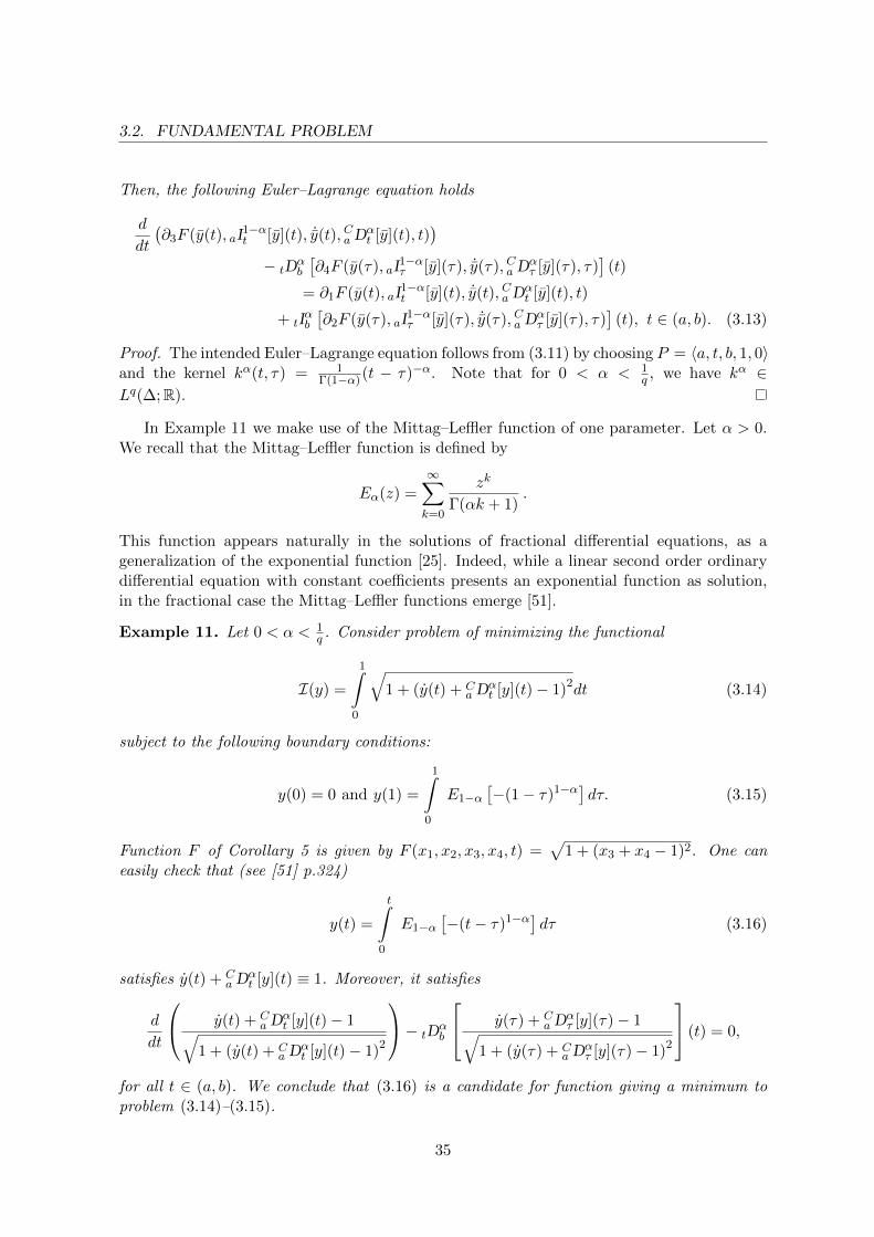
3.2. FUNDAMENTAL PROBLEM
Then, the following Euler–Lagrange equation holds
d
dt
(∂3F (y(t), aI
1−αt [y](t), ˙y(t), Ca D
αt [y](t), t)
)− tD
αb
[∂4F (y(τ), aI
1−ατ [y](τ), ˙y(τ), Ca D
ατ [y](τ), τ)
](t)
= ∂1F (y(t), aI1−αt [y](t), ˙y(t), Ca D
αt [y](t), t)
+ tIαb
[∂2F (y(τ), aI
1−ατ [y](τ), ˙y(τ), Ca D
ατ [y](τ), τ)
](t), t ∈ (a, b). (3.13)
Proof. The intended Euler–Lagrange equation follows from (3.11) by choosing P = 〈a, t, b, 1, 0〉and the kernel kα(t, τ) = 1
Γ(1−α)(t − τ)−α. Note that for 0 < α < 1q , we have kα ∈
Lq(∆;R).
In Example 11 we make use of the Mittag–Leffler function of one parameter. Let α > 0.We recall that the Mittag–Leffler function is defined by
Eα(z) =
∞∑k=0
zk
Γ(αk + 1).
This function appears naturally in the solutions of fractional differential equations, as ageneralization of the exponential function [25]. Indeed, while a linear second order ordinarydifferential equation with constant coefficients presents an exponential function as solution,in the fractional case the Mittag–Leffler functions emerge [51].
Example 11. Let 0 < α < 1q . Consider problem of minimizing the functional
I(y) =
1∫0
√1 + (y(t) + C
a Dαt [y](t)− 1)2dt (3.14)
subject to the following boundary conditions:
y(0) = 0 and y(1) =
1∫0
E1−α[−(1− τ)1−α] dτ. (3.15)
Function F of Corollary 5 is given by F (x1, x2, x3, x4, t) =√
1 + (x3 + x4 − 1)2. One caneasily check that (see [51] p.324)
y(t) =
t∫0
E1−α[−(t− τ)1−α] dτ (3.16)
satisfies y(t) + Ca D
αt [y](t) ≡ 1. Moreover, it satisfies
d
dt
y(t) + Ca D
αt [y](t)− 1√
1 + (y(t) + Ca D
αt [y](t)− 1)2
− tDαb
y(τ) + Ca D
ατ [y](τ)− 1√
1 + (y(τ) + Ca D
ατ [y](τ)− 1)2
(t) = 0,
for all t ∈ (a, b). We conclude that (3.16) is a candidate for function giving a minimum toproblem (3.14)–(3.15).
35

CHAPTER 3. STANDARD METHODS IN FRACTIONAL VARIATIONAL CALCULUS
Corollary 6 (cf. [3]). Let 0 < α < 1q and let I be the functional
I(y) =
b∫a
F(y(t), y(t), λ Ca D
αt [y](t) + µ Ct D
αb [y](t), t
)dt, (3.17)
where λ and µ are real numbers, and let y ∈ C1([a, b];R) be a minimizer of I among allfunctions satisfying boundary conditions y(a) = ya, y(b) = yb. Moreover, we assume that
• F ∈ C1(R3 × [a, b];R),
• functions t 7→ ∂2F(y(t), y(t), λ Ca D
αt [y](t) + µ Ct D
αb [y](t), t
),
aI1−αt
[∂3F
(y(τ), y(τ), λ Ca D
ατ [y](τ) + µ Cτ D
αb [y](τ), τ
)],
and tI1−αb
[∂3F
(y(τ), y(τ), λ Ca D
ατ [y](τ) + µ Cτ D
αb [y](τ), τ
)]are continuously differentiable
on [a, b].
Then, y satisfies the Euler–Lagrange equation
λ tDαb
[∂3F
(y(τ), ˙y(τ), λ Ca D
ατ [y](τ) + µ Cτ D
αb [y](τ), τ
)](t)
+ µ aDαt
[∂3F
(y(τ), ˙y(τ), λ Ca D
ατ [y](τ) + µ Cτ D
αb [y](τ), τ
)](t)
+ ∂1F(y(t), ˙y(t), λ Ca D
αt [y](t) + µ Ct D
αb [y](t), t
)− d
dt
(∂2F
(y(t), ˙y(t), λ Ca D
αt [y](t) + µ Ct D
αb [y](t), t
))= 0 (3.18)
for all t ∈ (a, b).
Proof. Choose P = 〈a, t, b, λ,−µ〉 and kα(t − τ) = 1Γ(1−α)(t − τ)−α. Then, for 0 < α < 1
q
kernel kα is in Lq(∆;R), the operator BP reduces to the sum of the left and right Caputofractional derivatives and (3.18) follows from (3.11).
Corollary 7. Let us consider the problem of minimizing a functional
I(y) =
b∫a
F(y(t), aI
1−α(·,·)t [y](t), y(t), Ca D
α(·,·)t [y](t), t
)dt (3.19)
subject to boundary conditions
y(a) = ya, y(b) = yb, (3.20)
where y, aI1−α(·,·)t [y], Ca D
α(·,·)t [y] ∈ C([a, b];R) and α : ∆→ [0, 1− δ] with δ > 1
p . Moreover, weassume that
• F ∈ C1(R4 × [a, b],R)
• function tI1−α(·,·)b
[∂2F
(y(τ), aI
1−α(·,·)τ [y](τ), y(τ), Ca D
α(·,·)τ [y](τ), τ
)]is continuous on [a, b],
• functions t 7→ ∂3F(y(t), aI
1−α(·,·)t [y](t), y, Ca D
α(·,·)t [y](t), t
)and tI
1−α(·,·)b
[∂4F
(y(τ), aI
1−α(·,·)τ [y](τ), y(τ), Ca D
α(·,·)τ [y](τ), τ
)]are continuously differ-
entiable on [a, b].
36
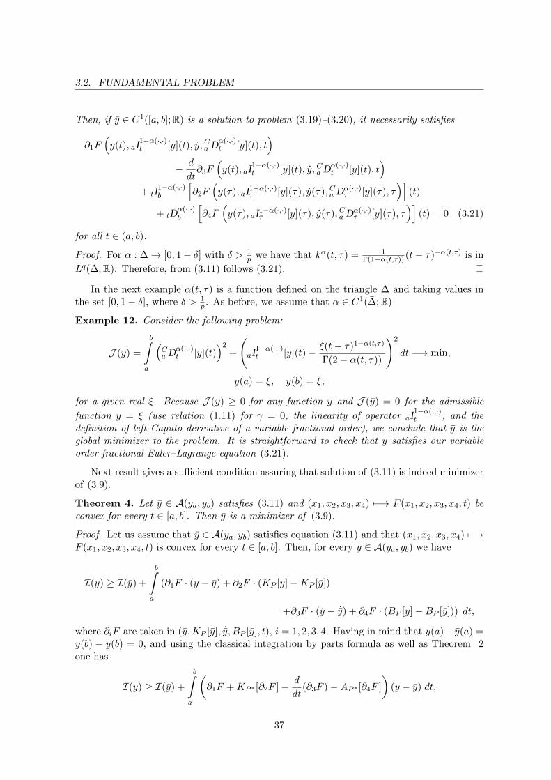
3.2. FUNDAMENTAL PROBLEM
Then, if y ∈ C1([a, b];R) is a solution to problem (3.19)–(3.20), it necessarily satisfies
∂1F(y(t), aI
1−α(·,·)t [y](t), y, Ca D
α(·,·)t [y](t), t
)− d
dt∂3F
(y(t), aI
1−α(·,·)t [y](t), y, Ca D
α(·,·)t [y](t), t
)+ tI
1−α(·,·)b
[∂2F
(y(τ), aI
1−α(·,·)τ [y](τ), y(τ), Ca D
α(·,·)τ [y](τ), τ
)](t)
+ tDα(·,·)b
[∂4F
(y(τ), aI
1−α(·,·)τ [y](τ), y(τ), Ca D
α(·,·)τ [y](τ), τ
)](t) = 0 (3.21)
for all t ∈ (a, b).
Proof. For α : ∆→ [0, 1− δ] with δ > 1p we have that kα(t, τ) = 1
Γ(1−α(t,τ))(t− τ)−α(t,τ) is in
Lq(∆;R). Therefore, from (3.11) follows (3.21).
In the next example α(t, τ) is a function defined on the triangle ∆ and taking values inthe set [0, 1− δ], where δ > 1
p . As before, we assume that α ∈ C1(∆;R)
Example 12. Consider the following problem:
J (y) =
b∫a
(Ca D
α(·,·)t [y](t)
)2+
(aI
1−α(·,·)t [y](t)− ξ(t− τ)1−α(t,τ)
Γ(2− α(t, τ))
)2
dt −→ min,
y(a) = ξ, y(b) = ξ,
for a given real ξ. Because J (y) ≥ 0 for any function y and J (y) = 0 for the admissible
function y = ξ (use relation (1.11) for γ = 0, the linearity of operator aI1−α(·,·)t , and the
definition of left Caputo derivative of a variable fractional order), we conclude that y is theglobal minimizer to the problem. It is straightforward to check that y satisfies our variableorder fractional Euler–Lagrange equation (3.21).
Next result gives a sufficient condition assuring that solution of (3.11) is indeed minimizerof (3.9).
Theorem 4. Let y ∈ A(ya, yb) satisfies (3.11) and (x1, x2, x3, x4) 7−→ F (x1, x2, x3, x4, t) beconvex for every t ∈ [a, b]. Then y is a minimizer of (3.9).
Proof. Let us assume that y ∈ A(ya, yb) satisfies equation (3.11) and that (x1, x2, x3, x4) 7−→F (x1, x2, x3, x4, t) is convex for every t ∈ [a, b]. Then, for every y ∈ A(ya, yb) we have
I(y) ≥ I(y) +
b∫a
(∂1F · (y − y) + ∂2F · (KP [y]−KP [y])
+∂3F · (y − ˙y) + ∂4F · (BP [y]−BP [y])) dt,
where ∂iF are taken in (y,KP [y], ˙y,BP [y], t), i = 1, 2, 3, 4. Having in mind that y(a)− y(a) =y(b) − y(b) = 0, and using the classical integration by parts formula as well as Theorem 2one has
I(y) ≥ I(y) +
b∫a
(∂1F +KP ∗ [∂2F ]− d
dt(∂3F )−AP ∗ [∂4F ]
)(y − y) dt,
37

CHAPTER 3. STANDARD METHODS IN FRACTIONAL VARIATIONAL CALCULUS
where, as before, ∂iF are taken in (y, KP [y], ˙y,BP [y], t), i = 1, 2, 3, 4. Finally, by Euler–Lagrange equation (3.11), we have I(y) ≥ I(y).
3.3 Free Initial Boundary
Let us define the following set
A(yb) :=y ∈ C1([a, b];R) : y(a) is free, y(b) = yb, and KP [y], BP [y] ∈ C([a, b];R)
,
and let y be a minimizer of functional (3.9) on A(yb), i.e., now
I : A(yb) −→ R
y 7−→b∫a
F (y(t),KP [y](t), y(t), BP [y](t), t) dt.
(3.22)
Because
I(y) ≤ I(y + hη),
for any |h| ≤ ε and every η ∈ A(0), we obtain as in the proof of Theorem 3 that
b∫a
(∂1F (?y)(t) +KP ∗ [∂2F (?y)(τ)] (t)) · η(t)
+ (∂3F (?y)(t) +KP ∗ [∂4F (?y)(τ)] (t)) · η(t) dt = 0, ∀η ∈ A(0),
where (?y)(t) = (y(t),KP [y](t), ˙y(t), BP [y](t), t). Moreover, having in mind that η(b) = 0 andusing the classical integration by parts formula, we find that
b∫a
(∂1F (?y)(t) +KP ∗ [∂2F (?y)(τ)] (t)− d
dt(∂3F (?y)(t) +KP ∗ [∂4F (?y)(τ)] (t))
)· η(t) dt
+ ∂3F (?y)(t) · η(t)|a + KP ∗ [∂4F (?y)(τ)] (t) · η(t)|a = 0, ∀η ∈ A(0).
Now, using the fundamental lemma of calculus of variations (see e.g., [44]) and the fact thatη(a) is arbitrary, we obtain
ddt [∂3F (?y)(t)] +AP ∗ [∂4F (?y)(τ)] (t) = ∂1F (?y)(t) +KP ∗ [∂2F (?y)(τ)] (t),
∂3F (?y)(t)|a + KP ∗ [∂4F (?y)(τ)] (t)|a = 0.
We have just proved the following result.
Theorem 5. If y ∈ A(yb) is a solution to the problem of minimizing functional (3.22) on theset A(yb), then y satisfies the Euler–Lagrange equation (3.11). Moreover, the extra boundarycondition
∂3F (?y)(t)|a + KP ∗ [∂4F (?y)(τ)] (t)|a = 0, (3.23)
holds, with (?y)(t) = (y(t),KP [y](t), ˙y(t), BP [y](t), t).
38

3.3. FREE INITIAL BOUNDARY
Similarly as it is in the theory of the classical calculus of variations we will call (3.23) thegeneralized fractional natural boundary condition.
Corollary 8 (cf. [2]). Let 0 < α < 1q and I be the functional given by
I(y) =
b∫a
F(y(t),Ca Dα
t [y](t), t)dt,
where F ∈ C1(R2 × [a, b];R), and aI1−αt
[∂2F
(y(τ),Ca Dα
τ [y](τ), τ)]
is continuously differen-tiable on [a, b]. If y ∈ C1([a, b];R) is a minimizer of I among all functions satisfying theboundary condition y(b) = yb, then y satisfies the Euler–Lagrange equation
∂1F(y(t),Ca Dα
t [y](t), t)
+t Dαb
[∂2F
(y(τ),Ca Dα
τ [y](τ), τ)]
(t) = 0
and the fractional natural boundary condition
tI1−αb
[∂2F
(y(τ),Ca Dα
τ [y](τ), τ)]
(t)∣∣a
= 0
holds for all t ∈ (a, b).
Proof. Corollary 8 follows from Theorem 5 with P = 〈a, t, b, 1, 0〉 and kα(t, τ) = 1Γ(1−α)(t −
τ)−α.
Corollary 9. Suppose that α : ∆→ [0, 1− δ], δ > 1p and I is the functional given by (3.19).
If y ∈ C1([a, b];R) is a minimizer to I satisfying boundary condition y(b) = yb and being such
that aI1−α(·,·)t [y], Ca D
α(·,·)t [y] ∈ C([a, b];R), then y is a solution to the Euler–Lagrange equation
∂1F(y(t), aI
1−α(·,·)t [y](t), ˙y, Ca D
α(·,·)t [y](t), t
)− d
dt∂3F
(y(t), aI
1−α(·,·)t [y](t), ˙y(t), Ca D
α(·,·)t [y](t), t
)+ tI
1−α(·,·)b
[∂2F
(y(τ), aI
1−α(·,·)τ [y](τ), y(τ), Ca D
α(·,·)τ [y](τ), τ
)](t)
+ tDα(·,·)b
[∂4F
(y(τ), aI
1−α(·,·)τ [y](τ), ˙y(τ), Ca D
α(·,·)τ [y](τ), τ
)](t) = 0
and the natural boundary condition
∂3F(y(t), aI
1−α(·,·)t [y](t), ˙y(t), Ca D
α(·,·)t [y](t), t
)∣∣∣a
+ tI1−α(·,·)b
[∂4F
(y(τ), aI
1−α(·,·)τ [y](τ), ˙y(τ), Ca D
α(·,·)τ [y](τ), τ
)](t)∣∣∣a
= 0
holds for all t ∈ (a, b).
Proof. Corollary 9 is an easy consequence of Theorem 5.
Remark 4. Observe that if the functional (3.22) is independent of the operator KP , that iswe have the following problem:
b∫a
F (y(t), y(t), BP [y](t), t) dt −→ min, y(b) = yb
39

CHAPTER 3. STANDARD METHODS IN FRACTIONAL VARIATIONAL CALCULUS
(y(a) free), then the optimality conditions (3.11) and (3.23) reduce, respectively, to
∂1F (y(t), ˙y(t), BP [y](t), t)− d
dt∂2F (y(t), ˙y(t), BP [y](t), t)
−AP ∗ [∂3F (y(τ), ˙y(τ), BP [y](τ), τ)] (t) = 0
and ∂2F (y(t), ˙y(t), BP [y](t), t)|a + KP ∗ [∂3F (y(τ), ˙y(τ), BP [y](τ), τ)] (t)|a = 0 for all t ∈(a, b).
3.4 Isoperimetric Problem
One of the earliest problems in geometry is the isoperimetric problem, already consideredby the ancient Greeks. It consists to find, among all closed curves of a given length, theone which encloses the maximum area. The general problem for which one integral is to begiven a fixed value, while another is to be made a maximum or a minimum, is nowadayspart of the calculus of variations [45, 104]. Such isoperimetric problems have found a broadclass of important applications throughout the centuries, with numerous useful implicationsin astronomy, geometry, algebra, analysis, and engineering [20, 32]. For recent advancementson the study of isoperimetric problems see [13,14,40] and references therein. Here we considerisoperimetric problems with generalized fractional operators. Similarly to Section 3.2 and 3.3,we deal with integrands involving both the generalized Caputo fractional derivative and thegeneralized fractional integral, as well as the classical derivative.
Let P = 〈a, t, b, λ, µ〉. We define the following functional:
J : A(ya, yb) −→ R
y 7−→b∫aG(y(t),KP [y](t), y(t), BP [y](t), t) dt,
(3.24)
where by y we understand the classical derivative of y, KP is the generalized fractional integraloperator with kernel belonging to Lq(∆;R), BP = KP d
dt and G is a Lagrangian of class C1:
G : R4 × [a, b] −→ R(x1, x2, x3, x4, t) 7−→ G(x1, x2, x3, x4, t).
Moreover, we assume that
• KP ∗ [∂2G(y(τ),KP [y](τ), y(τ), BP [y](τ), τ)] ∈ C([a, b];R),
• t 7→ ∂3G(y(t),KP [y](t), y(t), BP [y](t), t) ∈ C1([a, b];R),
• KP ∗ [∂4G(y(τ),KP [y](τ), y(τ), BP [y](τ), τ)] ∈ C1([a, b];R).
The first problem in this section, is to find a minimizer of functional (3.9) subject tothe isoperimetric constraint J (y) = ξ. In the next theorem we provide necessary optimalitycondition for this type of problems.
Theorem 6. Suppose that y is a minimizer of functional I in the class
Aξ(ya, yb) := y ∈ A(ya, yb) : J (y) = ξ .
40

3.4. ISOPERIMETRIC PROBLEM
Then there exists a real constant λ0, such that, for H = F − λ0G, equation
d
dt[∂3H(?y)(t)]+AP ∗ [∂4H(?y)(τ)] (t) = ∂1H(?y)(t)+KP ∗ [∂2H(?y)(τ)] (t), t ∈ (a, b) (3.25)
holds, provided that
d
dt[∂3G(?y)(t)] +AP ∗ [∂4G(?y)(τ)] (t) 6= ∂1G(?y)(t) +KP ∗ [∂2G(?y)(τ)] (t), t ∈ (a, b) (3.26)
where (?y)(t) = (y(t),KP [y](t), ˙y(t), BP [y](t), t).
Proof. By hypothesis (3.26) and the fundamental lemma of the calculus of variations (seee.g., [44]) we can choose η2 ∈ A(0, 0) so that
b∫a
(∂1G(?y)(t) +KP ∗ [∂2G(?y)(τ)] (t)) · η2(t)
+ (∂3G(?y)(t) +KP ∗ [∂4G(?y)(τ)] (t)) · η2(t) dt = 1.
With this function η2 and an arbitrary η1 ∈ A(0, 0), let us define functions
φ : [−ε1, ε1]× [−ε2, ε2] −→ R(h1, h2) 7−→ I(y + h1η1 + h2η2)
andψ : [−ε1, ε1]× [−ε2, ε2] −→ R
(h1, h2) 7−→ J (y + h1η1 + h2η2)− ξ.
Observe that ψ(0, 0) = 0 and
∂ψ
∂h2
∣∣∣∣(0,0)
=
b∫a
(∂1G(?y)(t) +KP ∗ [∂2G(?y)(τ)] (t)) · η2(t)
+ (∂3G(?y)(t) +KP ∗ [∂4G(?y)(τ)] (t)) · η2(t) dt = 1.
According to the implicit function theorem we can find ε0 > 0 and a function s ∈ C1([−ε0, ε0];R)with s(0) = 0 such that
ψ(h1, s(h1)) = 0, ∀h1 ∈ [−ε0, ε0]
which implies that y + h1η1 + s(h1)η2 ∈ Aξ(ya, yb). We also have
∂ψ
∂h1+∂ψ
∂h2· s′(h1) = 0, ∀h1 ∈ [−ε0, ε0]
and hence
s′(0) = − ∂ψ∂h1
∣∣∣∣(0,0)
.
Because y ∈ A(ya, yb) is a minimizer of I we have
φ(0, 0) ≤ φ(h1, s(h1)), ∀h1 ∈ [−ε0, ε0]
41

CHAPTER 3. STANDARD METHODS IN FRACTIONAL VARIATIONAL CALCULUS
and then∂φ
∂h1
∣∣∣∣(0,0)
+∂φ
∂h2
∣∣∣∣(0,0)
· s′(0) = 0.
Letting λ0 = ∂φ∂h2
∣∣∣(0,0)
be the Lagrange multiplier we find
∂φ
∂h1
∣∣∣∣(0,0)
− λ0∂ψ
∂h1
∣∣∣∣(0,0)
= 0
or, in other words,
b∫a
[(∂1F (?y)(t) +KP ∗ [∂2F (?y)(τ)] (t)) · η1(t) + (∂3F (?y)(t) +KP ∗ [∂4F (?y)(τ)] (t)) · η1(t)]
−λ0 [(∂1G(?y)(t) +KP ∗ [∂2G(?y)(τ)] (t)) · η1(t) + (∂3G(?y)(t) +KP ∗ [∂4G(?y)(τ)] (t)) · η1(t)] dt= 0.
Finally, applying one more time the fundamental lemma of the calculus of variations we obtain(3.25).
Example 13. Let P = 〈0, t, 1, 1, 0〉. Consider the problem
I(y) =
1∫0
(KP [y](t) + t)2 dt −→ min,
J (y) =
1∫0
tKP [y](t) dt = ξ,
y(0) = ξ − 1, y(1) = (ξ − 1)
1 +
1∫0
u(1− τ)dτ
,
where the kernel k is such that k(t, τ) = h(t − τ) with h ∈ C1([0, 1];R), h(0) = 1 andKP ∗ [id](t) 6= 0 (notation id means identity transformation i.e., id(t) = t). Here the resolventu is related to the kernel h in the same way as in Example 10. Since KP ∗ [id](t) 6= 0, thereis no solution to the Euler–Lagrange equation for functional J . The augmented LagrangianH of Theorem 6 is given by H(x1, x2, t) = (x2 + t)2 − λ0tx2. Function
y(t) = (ξ − 1)
1 +
t∫0
u(t− τ)dτ
is the solution to the Volterra integral equation of the first kind KP [y](t) = (ξ− 1)t (see, e.g.,Equation 16, p. 114 of [92]) and for λ0 = 2ξ satisfies our optimality condition (3.25):
KP ∗ [2 (KP [y](τ) + τ)− 2ξτ ] (t) = 0. (3.27)
The solution of (3.27) subject to the given boundary conditions depends on the particularchoice for the kernel. For example, let hα(t−τ) = eα(t−τ). Then the solution of (3.27) subject
42
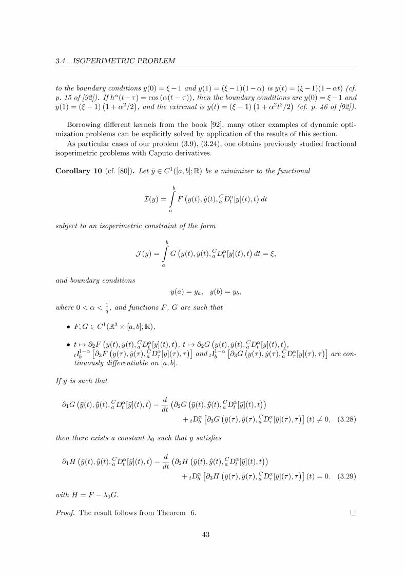
3.4. ISOPERIMETRIC PROBLEM
to the boundary conditions y(0) = ξ−1 and y(1) = (ξ−1)(1−α) is y(t) = (ξ−1)(1−αt) (cf.p. 15 of [92]). If hα(t−τ) = cos (α(t− τ)), then the boundary conditions are y(0) = ξ−1 andy(1) = (ξ − 1)
(1 + α2/2
), and the extremal is y(t) = (ξ − 1)
(1 + α2t2/2
)(cf. p. 46 of [92]).
Borrowing different kernels from the book [92], many other examples of dynamic opti-mization problems can be explicitly solved by application of the results of this section.
As particular cases of our problem (3.9), (3.24), one obtains previously studied fractionalisoperimetric problems with Caputo derivatives.
Corollary 10 (cf. [80]). Let y ∈ C1([a, b];R) be a minimizer to the functional
I(y) =
b∫a
F(y(t), y(t), Ca D
αt [y](t), t
)dt
subject to an isoperimetric constraint of the form
J (y) =
b∫a
G(y(t), y(t), Ca D
αt [y](t), t
)dt = ξ,
and boundary conditions
y(a) = ya, y(b) = yb,
where 0 < α < 1q , and functions F , G are such that
• F,G ∈ C1(R3 × [a, b];R),
• t 7→ ∂2F(y(t), y(t), Ca D
αt [y](t), t
), t 7→ ∂2G
(y(t), y(t), Ca D
αt [y](t), t
),
tI1−αb
[∂3F
(y(τ), y(τ), Ca D
ατ [y](τ), τ
)]and tI
1−αb
[∂3G
(y(τ), y(τ), Ca D
ατ [y](τ), τ
)]are con-
tinuously differentiable on [a, b].
If y is such that
∂1G(y(t), ˙y(t), Ca D
αt [y](t), t
)− d
dt
(∂2G
(y(t), ˙y(t), Ca D
αt [y](t), t
))+ tD
αb
[∂3G
(y(τ), ˙y(τ), Ca D
ατ [y](τ), τ
)](t) 6= 0, (3.28)
then there exists a constant λ0 such that y satisfies
∂1H(y(t), ˙y(t), Ca D
αt [y](t), t
)− d
dt
(∂2H
(y(t), ˙y(t), Ca D
αt [y](t), t
))+ tD
αb
[∂3H
(y(τ), ˙y(τ), Ca D
ατ [y](τ), τ
)](t) = 0. (3.29)
with H = F − λ0G.
Proof. The result follows from Theorem 6.
43

CHAPTER 3. STANDARD METHODS IN FRACTIONAL VARIATIONAL CALCULUS
Example 14. Let α ∈(
0, 1q
)and ξ ∈ R. Consider the following fractional isoperimetric
problem:
I(y) =
1∫0
(y(t) + C
0 Dαt [y](t)(t)
)2dt −→ min
J (y) =
1∫0
(y(t) + C
0 Dαt [y](t)
)dt = ξ
y(0) = 0, y(1) =
1∫0
E1−α
(− (1− τ)1−α
)ξdτ.
(3.30)
In our example (3.30) the function H of Corollary 10 is given by
H(y(t), y(t), C0 Dαt [y](t), t) =
(y(t) + C
0 Dαt [y](t)
)2 − λ0
(y(t) + C
0 Dαt [y](t)
).
One can easily check that function
y(t) =
∫ t
0E1−α
(− (t− τ)1−α
)ξdτ (3.31)
• is such that (3.28) holds;
• satisfies y(t) + C0 D
αt [y](t) = ξ (see, e.g., p. 328, Example 5.24 [51]).
Moreover, (3.31) satisfies the Euler–Lagrange equation (3.29) for λ0 = 2ξ, i.e.,
− d
dt
(2(y(t) + C
0 Dαt [y](t)
)− 2ξ
)+ tD
α1
[(2(y(τ) + C
0 Dατ [y](τ)
)− 2ξ
)]= 0
We conclude that (3.31) is an extremal for the isoperimetric problem (3.30).
Let us consider two cases.
1. Choose ξ = 1. When α→ 0 one gets from (3.30) the classical isoperimetric problem
I(y) =
1∫0
(y(t) + y(t))2 dt −→ min
J (y) =
1∫0
y(t)dt =1
e
y(0) = 0 y(1) = 1− 1
e.
(3.32)
Our extremal (3.31) is then reduced to the classical extremal y(t) = 1 − e−t of theisoperimetric problem (3.32).
44

3.4. ISOPERIMETRIC PROBLEM
2. Let α = 12 . Then (3.30) gives the following fractional isoperimetric problem:
I(y) =
1∫0
(y(t) + C
0 D12t [y](t)
)2
dt −→ min
J (y) =
1∫0
(y(t) + C
0 D12t [y](t)
)dt = ξ
y(0) = 0 , y(1) = ξ
(erfc(1)e +
2√π− 1
),
(3.33)
where erfc is the complementary error function defined by
erfc(z) =2√π
∞∫z
exp(−t2)dt.
The extremal (3.31) for the particular fractional isoperimetric problem (3.33) is
y(t) = ξ
(eterfc(
√t)− 2
√t√π− 1
).
Corollary 11. Let us consider the problem of minimizing functional (3.19) subject to anisoperimetric constraint
J (y) =
b∫a
G(y(t), aI
1−α(·,·)t [y](t), y(t), Ca D
α(·,·)t [y](t), t
)dt = ξ (3.34)
and the boundary conditionsy(a) = ya, y(b) = yb, (3.35)
where y, aI1−α(·,·)t [y], Ca D
α(·,·)t [y] ∈ C([a, b];R) and α : ∆→ [0, 1− δ] with δ > 1
p . Moreover, weassume that
• G ∈ C1(R4 × [a, b];R),
• tI1−α(·,·)b
[∂2G
(y(τ), aI
1−α(·,·)τ [y](τ), y(τ), Ca D
α(·,·)τ [y](τ), τ
)]is continuous on [a, b],
• t 7→ ∂3G(y(t), aI
1−α(·,·)t [y](t), y(t), Ca D
α(·,·)t [y](t), t
)and , tI
1−α(·,·)b
[∂4G
(y(τ), aI
1−α(·,·)τ [y](τ), y(τ), Ca D
α(·,·)τ [y](τ), τ
)]are continuously differ-
entiable on [a, b].
If y ∈ C1([a, b];R) is a solution to problem (3.19),(3.34),(3.35), then there exists realnumber λ0 such that, for H = F − λ0G, we have
∂1H −d
dt∂3H + tI
1−α(t,·)b [∂2H] + tD
α(t,·)b [∂4H] = 0,
provided that
∂1G−d
dt∂3G+ tI
1−α(t,·)b [∂2G] + tD
α(t,·)b [∂4G] 6= 0.
Here, functions ∂iH and ∂iG, i = 1, 2, 3, 4, are evaluated at(y(t), aI
1−α(·,·)t [y](t), ˙y, Ca D
α(·,·)t [y](t), t
).
45
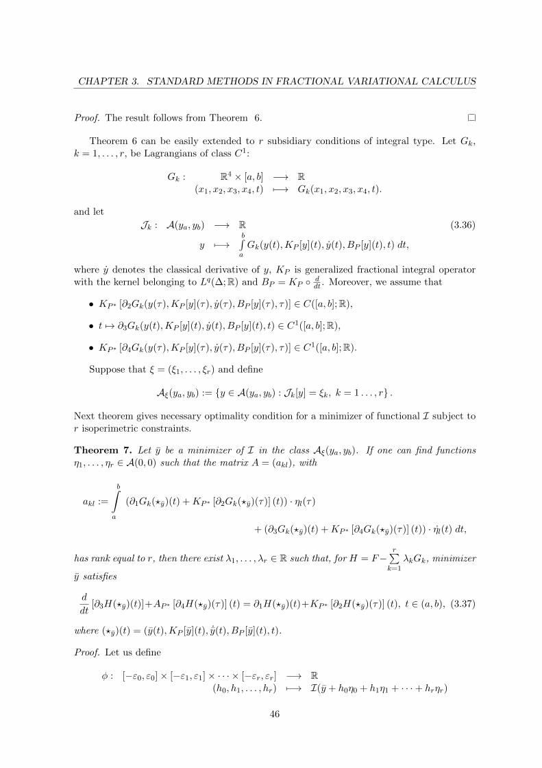
CHAPTER 3. STANDARD METHODS IN FRACTIONAL VARIATIONAL CALCULUS
Proof. The result follows from Theorem 6.
Theorem 6 can be easily extended to r subsidiary conditions of integral type. Let Gk,k = 1, . . . , r, be Lagrangians of class C1:
Gk : R4 × [a, b] −→ R(x1, x2, x3, x4, t) 7−→ Gk(x1, x2, x3, x4, t).
and let
Jk : A(ya, yb) −→ R
y 7−→b∫aGk(y(t),KP [y](t), y(t), BP [y](t), t) dt,
(3.36)
where y denotes the classical derivative of y, KP is generalized fractional integral operatorwith the kernel belonging to Lq(∆;R) and BP = KP d
dt . Moreover, we assume that
• KP ∗ [∂2Gk(y(τ),KP [y](τ), y(τ), BP [y](τ), τ)] ∈ C([a, b];R),
• t 7→ ∂3Gk(y(t),KP [y](t), y(t), BP [y](t), t) ∈ C1([a, b];R),
• KP ∗ [∂4Gk(y(τ),KP [y](τ), y(τ), BP [y](τ), τ)] ∈ C1([a, b];R).
Suppose that ξ = (ξ1, . . . , ξr) and define
Aξ(ya, yb) := y ∈ A(ya, yb) : Jk[y] = ξk, k = 1 . . . , r .
Next theorem gives necessary optimality condition for a minimizer of functional I subject tor isoperimetric constraints.
Theorem 7. Let y be a minimizer of I in the class Aξ(ya, yb). If one can find functionsη1, . . . , ηr ∈ A(0, 0) such that the matrix A = (akl), with
akl :=
b∫a
(∂1Gk(?y)(t) +KP ∗ [∂2Gk(?y)(τ)] (t)) · ηl(τ)
+ (∂3Gk(?y)(t) +KP ∗ [∂4Gk(?y)(τ)] (t)) · ηl(t) dt,
has rank equal to r, then there exist λ1, . . . , λr ∈ R such that, for H = F−r∑
k=1
λkGk, minimizer
y satisfies
d
dt[∂3H(?y)(t)]+AP ∗ [∂4H(?y)(τ)] (t) = ∂1H(?y)(t)+KP ∗ [∂2H(?y)(τ)] (t), t ∈ (a, b), (3.37)
where (?y)(t) = (y(t),KP [y](t), ˙y(t), BP [y](t), t).
Proof. Let us define
φ : [−ε0, ε0]× [−ε1, ε1]× · · · × [−εr, εr] −→ R(h0, h1, . . . , hr) 7−→ I(y + h0η0 + h1η1 + · · ·+ hrηr)
46

3.5. NOETHER’S THEOREM
and
ψk : [−ε0, ε0]× [−ε1, ε1]× · · · × [−εr, εr] −→ R(h0, h1, . . . , hr) 7−→ Jk(y + h0η0 + h1η1 + · · ·+ hrηr)− ξk
Observe that φ, ψk are functions of class C1 ([−ε0.ε0]× · · · × [−εr, εr];R), A =(∂ψk∂hl
∣∣∣0
)and
that ψk(0, 0, . . . , 0) = 0. Moreover, because y is a minimizer of functional I we have
φ(0, . . . , 0) ≤ φ(h0, h1, . . . , hr).
From the classical multiplier theorem, there are λ1, . . . , λr ∈ R such that
∇φl(0, . . . , 0) +
r∑k=1
λk∇ψk(0, . . . , 0) = 0, (3.38)
From (3.38), we can compute λ1, . . . , λr, turning out to be independent of the choice ofη0 ∈ A(0, 0). Finally, by the fundamental lemma of the calculus of variations, we arrive to(3.37).
3.5 Noether’s Theorem
Emmy Noether’s classical work [74] from 1918 states that a conservation law in variationalmechanics follow whenever the Lagrangian function is invariant under a one–parameter con-tinuous group of transformations, that transform dependent and/or independent variables.This result not only unifies conservation laws but also suggests a way to discover new ones.In this section we consider variational problems that depend on generalized fractional inte-grals and derivatives. Following the methods used in [29, 42, 43, 48]we apply Euler–Lagrangeequations to formulate a generalized fractional version of Noether’s theorem without trans-formation of time. We start by introducing the notion generalized fractional extremal andone–parameter family of infinitesimal transformations.
Definition 23. The function y ∈ C1 ([a, b];R), with KP [y], BP [y] ∈ C ([a, b];R), that is asolution to equation (3.11) is said to be a generalized fractional extremal.
We consider a one–parameter family of transformations of the form y(t) = φ(θ, t, y(t)),where φ is a map of class C2:
φ : [−ε, ε]× [a, b]× R −→ R(θ, t, x) 7−→ φ(θ, t, x),
such that φ(0, t, x) = x. Note that, using Taylor’s expansion of φ(θ, t, y(t)) in a neighborhoodof 0 one has
y(t) = φ(0, t, y(t)) + θ∂
∂θφ(0, t, y(t)) + o(θ),
provided that θ ∈ [−ε, ε]. Moreover, having in mind that φ(0, t, y(t)) = y(t) and denotingξ(t, y(t)) = ∂
∂θφ(0, t, y(t)), one has
y(t) = y(t) + θξ(t, y(t)) + o(θ), (3.39)
47

CHAPTER 3. STANDARD METHODS IN FRACTIONAL VARIATIONAL CALCULUS
so that, for θ ∈ [−ε, ε] the linear approximation to the transformation is
y(t) ≈ y(t) + θξ(t, y(t)).
Now, let us introduce the notion of invariance.
Definition 24. We say that the Lagrangian F is invariant under the one–parameter familyof infinitesimal transformations (3.39), where ξ is such that t 7→ ξ(t, y(t)) ∈ C1 ([a, b];R) withKP [τ 7→ ξ(τ, y(τ))] , BP [τ 7→ ξ(τ, y(τ))] ∈ C ([a, b];R) if
F (y(t),KP [y](t), y(t), BP [y](t), t) = F(y(t),KP [y](t), ˙y(t), BP [y](t), t
), (3.40)
for all θ ∈ [−ε, ε], and all y ∈ C1 ([a, b];R) with KP [y], BP [y] ∈ C ([a, b];R).
In order to state Noether’s theorem in a compact form, we introduce the following twobilinear operators:
D[f, g] := f ·AP ∗ [g] + g ·BP [f ], (3.41)
I[f, g] := −f ·KP ∗ [g] + g ·KP [f ]. (3.42)
Theorem 8 (Generalized Fractional Noether’s Theorem). Let F be invariant under the oneparameter family of infinitesimal transformations (3.39). Then for every generalized fractionalextremal the following equality holds
d
dt(ξ(t, y(t)) · ∂3F (?y)(t))+D [ξ(t, y(t)), ∂4F (?y)(t)]+I [ξ(t, y(t)), ∂2F (?y)(t)] = 0, t ∈ (a, b),
(3.43)where (?y)(t) = (y(t),KP [y](t), y(t), BP [y](t), t).
Proof. By equation (3.40) one has
d
dθ
[F(y(t),KP [y](t), ˙y(t), BP [y](t), t
)]∣∣∣∣θ=0
= 0
The usual chain rule implies
∂1F (?y)(t) ·d
dθy(t) + ∂2F (?y)(t) ·
d
dθKP [y](t)
+ ∂3F (?y)(t) ·d
dθ˙y(t) + ∂4F (?y)(t) ·
d
dθBP [y](t)
∣∣∣∣∣θ=0
= 0.
By linearity of KP , BP differentiating with respect to θ, and putting θ = 0 we have
∂1F (?y)(t) · ξ(t, y(t)) + ∂2F (?y)(t) ·KP [τ 7→ ξ(τ, y(τ))](t)
+ ∂3F (?y)(t) ·d
dtξ(t, y(t)) + ∂4F (?y)(t) ·BP [τ 7→ ξ(τ, y(τ))](t) = 0.
Now, using generalized Euler–Lagrange equation (3.11) and formulas (3.41) and (3.42) onearrives to (3.43).
48

3.5. NOETHER’S THEOREM
Example 15. Let P = 〈a, t, b, λ, µ〉 and y ∈ C1 ([a, b];R) with BP [y] ∈ C ([a, b];R). ConsiderLagrangian F (BP [y](t), t) and transformations
y(t) = y(t) + εc+ o(ε), (3.44)
where c is a constant. Then, we have
F (BP [y](t), t) = F (BP [y](t), t)
Therefore, F is invariant under (3.44) and the generalized fractional Noether’s theorem indi-cates that
AP ∗ [∂1F (BP [y](τ), τ)](t) = 0, t ∈ (a, b), (3.45)
along any generalized fractional extremal y. Notice that equation (3.45) can be written in theform
d
dt(KP ∗ [∂1F (BP [y](τ), τ)](t)) = 0, (3.46)
that is, quantity KP ∗ [∂1F (BP [y](τ), τ)] is conserved along all generalized fractional extremalsand this quantity, following the classical approach, can be called a generalized fractional con-stant of motion.
Similarly to previous sections, one can obtain from Theorem 8 results regarding to constantand variable order fractional integrals and derivatives.
Corollary 12. If for any y ∈ C1([a, b];R) the following equality is satisfied
F(y(t), y(t), λ Ca D
αt [y](t) + µ Ct D
αb [y](t), t
)= F
(y(t), ˙y(t), λ Ca D
αt [y](t) + µ Ct D
αb [y](t), t
),
where y is the family (3.39), then we have
d
dt
(ξ(t, y(t)) · ∂2F
(y(t), y(t), λ Ca D
αt [y](t) + µ Ct D
αb [y](t), t
))− ξ(t, y(t)) ·
(λtD
αb
[∂3F
(y(τ), y(τ), λ Ca D
ατ [y](τ) + µ Cτ D
αb [y](τ), τ
)](t)
µaDαt
[∂3F
(y(τ), y(τ), λ Ca D
ατ [y](τ) + µ Cτ D
αb [y](τ), τ
)](t))
+∂3F(y(t), y(t), λ Ca D
αt [y](t) + µ Ct D
αb [y](t), t
)·(λCa D
αt [ξ(τ, y(τ))](t) + µCt D
αb [ξ(τ, y(τ))](t)
)= 0
along all solutions of the Euler–Lagrange equation (3.18).
Proof. Corollary 12 is a simple consequence of Theorem 8.
Corollary 13. Let y ∈ C1([a, b];R) with I1−α(·,·)t [y], Ca D
α(·,·)t [y] ∈ C([a, b];R) and suppose that
F(y(t), aI
1−α(·,·)t [y](t), y(t), Ca D
α(·,·)t [y](t), t
)= F
(y(t), aI
1−α(·,·)t [y](t), ˙y(t), Ca D
α(·,·)t [y](t), t
)where y is the family (3.39) such that t 7→ ξ(t, y(t)) ∈ C1([a, b];R) and I
1−α(·,·)t [τ 7→ ξ(τ, y(τ))],
Ca D
α(·,·)t [τ 7→ ξ(τ, y(τ))] ∈ C([a, b];R). Then all solutions of the Euler–Lagrange equation
49
CHAPTER 3. STANDARD METHODS IN FRACTIONAL VARIATIONAL CALCULUS
(3.21) must satisfy
d
dt
(ξ(t, y(t)) · ∂3F
(y(t), aI
1−α(·,·)t [y](t), y(t), Ca D
α(·,·)t [y](t), t
))− ξ(t, y(t)) · tDα(·,·)
b
[∂4F
(y(τ), aI
1−α(·,·)τ [y](τ), y(τ), Ca D
α(·,·)τ [y](τ), τ
)](t)
+ ∂4F(y(t), aI
1−α(·,·)t [y](t), y(t), Ca D
α(·,·)t [y](t), t
)· Ca D
α(·,·)t [ξ(τ, y(τ))](t)
− ξ(t, y(t)) · tI1−α(·,·)b
[∂2F
(y(τ), aI
1−α(·,·)τ [y](τ), y(τ), Ca D
α(·,·)τ [y](τ), τ
)](t)
+ ∂2F(y(t), aI
1−α(·,·)t [y](t), y(t), Ca D
α(·,·)t [y](t), t
)· aI1−α(·,·)
t [ξ(τ, y(τ))](t) = 0, t ∈ (a, b).
Proof. Corollary 13 can be easily obtained from Theorem 8.
Corollary 14. Suppose that y ∈ C1([a, b];R) and for family (3.39) one has
F (y(t), aI1−αt [y](t), y(t), Ca D
αt [y](t), t) dt = F (y(t), aI
1−αt [y](t), ˙y(t), Ca D
αt [y](t), t).
Then
d
dt
(ξ(t, y(t)) · ∂2F (y(t), aI
1−αt [y](t), y(t), Ca D
αt [y](t), t)
)− ξ(t, y(t)) · tDα
b [∂4F (y(τ), aI1−ατ [y](τ), y(τ), Ca D
ατ [y](τ), τ)]
+ ∂4F (y(t), aI1−αt [y](t), y(t), Ca D
αt [y](t), t) · Ca Dα
t [ξ(τ, y(τ))]
− ξ(t, y(t)) · tI1−αb [∂2F (y(τ), aI1−ατ [y](τ), y(τ), Ca D
ατ [y](τ), τ)]
+ ∂2F (y(t), aI1−αt [y](t), y(t), Ca D
αt [y](t), t) · aI1−αt [ξ(τ, y(τ))] = 0
along any solution of the Euler–Lagrange equation (3.13).
Proof. Corollary 14 can be easily obtained from Theorem 8.
3.6 Variational Calculus in Terms of a Generalized Integral
In this section, we develop a generalized fractional calculus of variations, by consideringvery general problems, where the classical integrals are substituted by generalized fractionalintegrals, and the Lagrangians depend not only on classical derivatives but also on generalizedfractional operators. By choosing particular operators and kernels, one obtains the recentresults available in the literature of mathematical physics [35,36,46].
Let R = 〈a, b, b, 1, 0〉, P = 〈a, t, b, λ, µ〉 and consider the problem of finding a function ythat gives minimum value to the functional
I : A(ya, yb) −→ Ry 7−→ KR [F (y(t),KP [y](t), y(t), BP [y](t), t)] (b),
(3.47)
where KR and KP are generalized fractional integrals with kernels k(x, t) and h(t, τ), respec-tively, being elements of Lq(∆;R), BP = KP d
dt and F is a Lagrangian of class C1:
F : R4 × [a, b] −→ R(x1, x2, x3, x4, t) 7−→ F (x1, x2, x3, x4, t).
Moreover, we assume that
50
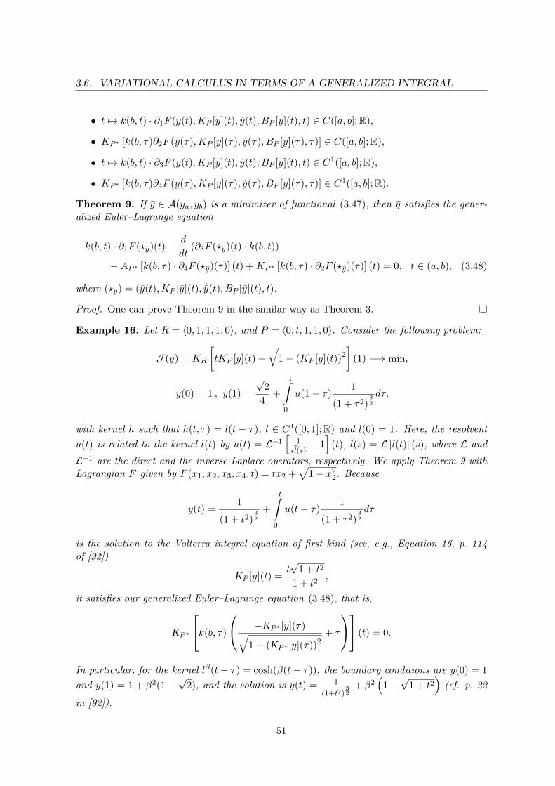
3.6. VARIATIONAL CALCULUS IN TERMS OF A GENERALIZED INTEGRAL
• t 7→ k(b, t) · ∂1F (y(t),KP [y](t), y(t), BP [y](t), t) ∈ C([a, b];R),
• KP ∗ [k(b, τ)∂2F (y(τ),KP [y](τ), y(τ), BP [y](τ), τ)] ∈ C([a, b];R),
• t 7→ k(b, t) · ∂3F (y(t),KP [y](t), y(t), BP [y](t), t) ∈ C1([a, b];R),
• KP ∗ [k(b, τ)∂4F (y(τ),KP [y](τ), y(τ), BP [y](τ), τ)] ∈ C1([a, b];R).
Theorem 9. If y ∈ A(ya, yb) is a minimizer of functional (3.47), then y satisfies the gener-alized Euler–Lagrange equation
k(b, t) · ∂1F (?y)(t)−d
dt(∂3F (?y)(t) · k(b, t))
−AP ∗ [k(b, τ) · ∂4F (?y)(τ)] (t) +KP ∗ [k(b, τ) · ∂2F (?y)(τ)] (t) = 0, t ∈ (a, b), (3.48)
where (?y) = (y(t),KP [y](t), ˙y(t), BP [y](t), t).
Proof. One can prove Theorem 9 in the similar way as Theorem 3.
Example 16. Let R = 〈0, 1, 1, 1, 0〉, and P = 〈0, t, 1, 1, 0〉. Consider the following problem:
J (y) = KR
[tKP [y](t) +
√1− (KP [y](t))2
](1) −→ min,
y(0) = 1 , y(1) =
√2
4+
1∫0
u(1− τ)1
(1 + τ2)32
dτ,
with kernel h such that h(t, τ) = l(t − τ), l ∈ C1([0, 1];R) and l(0) = 1. Here, the resolvent
u(t) is related to the kernel l(t) by u(t) = L−1[
1
sl(s)− 1]
(t), l(s) = L [l(t)] (s), where L and
L−1 are the direct and the inverse Laplace operators, respectively. We apply Theorem 9 withLagrangian F given by F (x1, x2, x3, x4, t) = tx2 +
√1− x2
2. Because
y(t) =1
(1 + t2)32
+
t∫0
u(t− τ)1
(1 + τ2)32
dτ
is the solution to the Volterra integral equation of first kind (see, e.g., Equation 16, p. 114of [92])
KP [y](t) =t√
1 + t2
1 + t2,
it satisfies our generalized Euler–Lagrange equation (3.48), that is,
KP ∗
k(b, τ)
−KP ∗ [y](τ)√1− (KP ∗ [y](τ))2
+ τ
(t) = 0.
In particular, for the kernel lβ(t− τ) = cosh(β(t− τ)), the boundary conditions are y(0) = 1
and y(1) = 1 + β2(1−√
2), and the solution is y(t) = 1
(1+t2)32
+ β2(
1−√
1 + t2)
(cf. p. 22
in [92]).
51

CHAPTER 3. STANDARD METHODS IN FRACTIONAL VARIATIONAL CALCULUS
The following corollary gives an extension of the main result of [37].
Corollary 15. If y ∈ C1 ([a, b];R) is a solution to the problem of minimizing
J (y) = aIαb
[F(y(t), y(t), CaD
βt [y] (t), t
)](b),
subject to the boundary conditions
y(a) = ya, y(b) = yb,
where α, β ∈ (0, 1q ), F ∈ C2
(R3 × [a, b];R
), then
∂1F(y(t), ˙y(t), CaD
βt [y] (t), t
)· (b− t)α−1
− d
dt
(∂2F
(y(t), ˙y(t), CaD
βt [y] (t), t
)· (b− t)α−1
)+ tD
βb
[(b− τ)α−1 · ∂3F
(y(τ), ˙y(τ), CaD
βτ [y] (τ), τ
)]= 0, t ∈ (a, b).
If the Lagrangian of functional (3.47) does not depend on generalized fractional operatorsB and K, then Theorem 9 gives the following result: if y ∈ C1([a, b];R) is a solution to theproblem of extremizing
I(y) =
∫ b
aF (y(t), y(t), t) k(b, t)dt (3.49)
subject to y(a) = ya and y(b) = yb, then
∂1F (y(t), y(t), t)− d
dt∂2F (y(t), y(t), t) =
1
k(b, t)· ddtk(b, t)∂2F (y(t), y(t), t) . (3.50)
We recognize on the right hand side of (3.50) the generalized weak dissipative parameter
δ(t) =1
(b, t)· ddtk(b, t).
Now, let us consider two examples of Lagrangians associated to functional (3.49).
Example 17. As a first example, let us consider kernel kα(b, t) = eα(b−t) and the Lagrangian
L (y(t), y(t), t) =1
2my2(t)− V (y(t)),
where V (y) is the potential energy and m stands for mass. The Euler–Lagrange equation(3.50) gives the following second-order ordinary differential equation:
y(t)− αy(t) = − 1
mV ′(y(t)). (3.51)
Equation (3.51) coincides with (14) of [46], obtained by modification of Hamilton’s principle.
Next example extends some of the recent results of [35,36], where the fractional action-likevariational approach (FALVA) was proposed to model dynamical systems. FALVA functionalsare particular cases of (3.49), where the fractional time integral introduces only one parameterα.
52

3.7. GENERALIZED VARIATIONAL CALCULUS OF SEVERAL VARIABLES
Example 18. Let us consider the Caldirola–Kanai Lagrangian [35, 36]
L (y(t), y(t), t) = m(t)
(y2(t)
2− ω2 y
2(t)
2
), (3.52)
which describes a dynamical oscillatory system with exponentially increasing time-dependentmass, where ω is the frequency and m(t) = m0e−γbeγt = m0eγt, m0 = m0e−γb. Using ourgeneralized FALVA Euler–Lagrange equation (3.50) with kernel k(b, t) to Lagrangian (3.52),we obtain
y(t) + (δ(t) + γ) y(t) + ω2y(t) = 0. (3.53)
We note that there is a small inconsistence in [35], regarding the coefficient of y(t) in(3.53).
3.7 Generalized Variational Calculus of Several Variables
Variational problems with functionals depending on several variables arise, for example,in mechanics problems, which involve systems with infinite number of degrees of freedom,like a vibrating elastic solid. Fractional variational problems involving multiple integrals havebeen already studied in different contexts. We can mention here [8, 17, 29, 77] where themutlidimensional fractional Euler–Lagrange equations for a field were obtained, or [68] wherefirst and second fractional Noether–type theorems are proved. In this section we present amore general approach to the subject by considering functionals depending on generalizedfractional operators.
3.7.1 Multidimensional Generalized Fractional Integration by Parts
In this section, it is of our interest to obtain integration by parts formula for generalizedfractional operators. We shall denote by t = (t1, . . . , tn) a point in Ωn, where Ωn = (a1, b1)×· · · × (an, bn), and by dt = dt1 . . . dtn. Throughout this subsection i ∈ 1, . . . , n is arbitrarybut fixed.
Theorem 10. Let Pi = 〈ai, ti, bi, λi, µi〉 be the parameter set and let KPi be the generalizedpartial fractional integral with ki being a difference kernel such that ki ∈ L1(0, bi − ai;R). Iff : Rn → R and η : Rn → R, f, η ∈ C
(Ωn;R
), then the generalized partial fractional integrals
satisfy the following identity:∫Ωn
f(t) ·KPi [η](t) dt =
∫Ωn
η(t) ·KP ∗i[f ](t) dt,
where P ∗i is the dual of Pi.
Proof. Let Pi = 〈ai, ti, bi, λi, µi〉 and f, η,∈ C(Ωn;R
). Since f and η, are continuous functions
on Ωn, they are bounded on Ωn i.e., there exist real numbers C,D > 0 such that |f(t)| ≤ C,
53
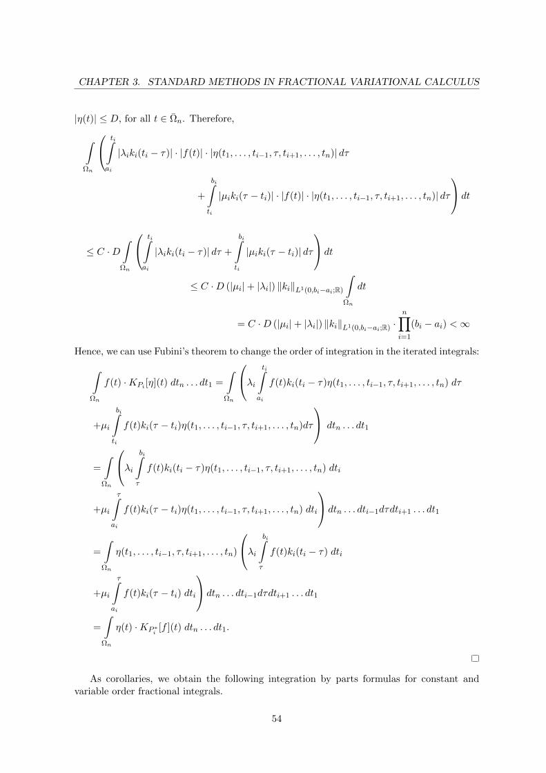
CHAPTER 3. STANDARD METHODS IN FRACTIONAL VARIATIONAL CALCULUS
|η(t)| ≤ D, for all t ∈ Ωn. Therefore,
∫Ωn
ti∫ai
|λiki(ti − τ)| · |f(t)| · |η(t1, . . . , ti−1, τ, ti+1, . . . , tn)| dτ
+
bi∫ti
|µiki(τ − ti)| · |f(t)| · |η(t1, . . . , ti−1, τ, ti+1, . . . , tn)| dτ
dt
≤ C ·D∫
Ωn
ti∫ai
|λiki(ti − τ)| dτ +
bi∫ti
|µiki(τ − ti)| dτ
dt
≤ C ·D (|µi|+ |λi|) ‖ki‖L1(0,bi−ai;R)
∫Ωn
dt
= C ·D (|µi|+ |λi|) ‖ki‖L1(0,bi−ai;R) ·n∏i=1
(bi − ai) <∞
Hence, we can use Fubini’s theorem to change the order of integration in the iterated integrals:∫Ωn
f(t) ·KPi [η](t) dtn . . . dt1 =
∫Ωn
λi ti∫ai
f(t)ki(ti − τ)η(t1, . . . , ti−1, τ, ti+1, . . . , tn) dτ
+µi
bi∫ti
f(t)ki(τ − ti)η(t1, . . . , ti−1, τ, ti+1, . . . , tn)dτ
dtn . . . dt1
=
∫Ωn
λi bi∫τ
f(t)ki(ti − τ)η(t1, . . . , ti−1, τ, ti+1, . . . , tn) dti
+µi
τ∫ai
f(t)ki(τ − ti)η(t1, . . . , ti−1, τ, ti+1, . . . , tn) dti
dtn . . . dti−1dτdti+1 . . . dt1
=
∫Ωn
η(t1, . . . , ti−1, τ, ti+1, . . . , tn)
λi bi∫τ
f(t)ki(ti − τ) dti
+µi
τ∫ai
f(t)ki(τ − ti) dti
dtn . . . dti−1dτdti+1 . . . dt1
=
∫Ωn
η(t) ·KP ∗i[f ](t) dtn . . . dt1.
As corollaries, we obtain the following integration by parts formulas for constant andvariable order fractional integrals.
54
3.7. GENERALIZED VARIATIONAL CALCULUS OF SEVERAL VARIABLES
Corollary 16. Let 0 < αi < 1, and let f : Rn → R, η : Rn → R be such that f, η ∈ C(Ωn;R),then the following formula holds∫
Ωn
f(t) · aiIαiti
[η](t) dt =
∫Ωn
η(t) · tiIαibi
[f ](t) dt. (3.54)
Corollary 17. Suppose that α : [0, bi − ai] → [0, 1], and that f : Rn → R, η : Rn → R aresuch that f, η ∈ C(Ωn;R). Then,∫
Ωn
f(t) · aiIαi(·)ti
[η](t) dt =
∫Ωn
η(t) · tiIαi(·)bi
[f ](t) dt. (3.55)
Theorem 11 (Generalized Fractional Integration by Parts for Several Variables). Let Pi =〈ai, ti, bi, λi, µi〉 be the parameter set and f, η ∈ C1
(Ωn;R
). Moreover, let BPi = d
dt KPi,where KPi is the generalized partial fractional integral with difference kernel i.e., ki = ki(ti−τ)such that ki ∈ L1(0, bi − ai;R), and KP ∗i
[f ] ∈ C1(Ωn;R
). Then∫
Ωn
f(t) ·BPi [η](t) dt =
∫∂Ωn
η(t) ·KP ∗i[f ](t) · νi d(∂Ωn)−
∫Ωn
η(t) ·AP ∗i [f ](t) dt,
where νi is the outward pointing unit normal to ∂Ωn.
Proof. By the definition of generalized partial Caputo fractional derivative, Theorem 10 andthe standard integration by parts formula (see e.g., [38]) one has∫
Ωn
f(t) ·BPi [η](t) dt =
∫Ωn
f(t) ·KPi
[∂η
∂ti
](t) dt =
∫Ωn
∂η(t)
∂ti·KP ∗i
[f ](t) dt
=
∫∂Ωn
η(t) ·KP ∗i[f ](t) · νi d(∂Ωn)−
∫Ωn
η(t) · ∂∂ti
KP ∗i[f ](t) dt
=
∫∂Ωn
η(t) ·KP ∗i[f ](t) · νi d(∂Ωn)−
∫Ωn
η(t) ·AP ∗i [f ](t) dt.
Next corollaries present multidimensional integration by parts formulas for constant andvariable order fractional derivatives.
Corollary 18. If 0 < αi < 1, functions f : Rn → R and η : Rn → R are such thatf, η ∈ C1(Ωn;R) and tI
1−αibi
[f ] ∈ C1(Ωn;R), then∫Ωn
f(t) · CaiDαiti
[η](t) dt =
∫∂Ωn
η(t) · tI1−αibi[f ](t) · νi d(∂Ωn)−
∫Ωn
η(t) · tiDαibi
[f ](t) dt.
Corollary 19. If αi : [0, bi−ai]→ [0, 1], functions f : Rn → R and η : Rn → R are such that
f, η ∈ C1(Ωn;R) and tiIαi(·)bi
[f ] ∈ C1(Ωn;R), then∫Ωn
f(t) · CaiDαi(·)ti
[η](t) dt =
∫∂Ωn
η(t) · tiIαi(·)bi
[f ](t) · νi d(∂Ωn)−∫
Ωn
η · tiDαi(·)bi
[f ](t) dt.
55
CHAPTER 3. STANDARD METHODS IN FRACTIONAL VARIATIONAL CALCULUS
3.7.2 Fundamental Problem
In this subsection, we use the notion of generalized fractional gradient.
Definition 25. Let n ∈ N and P = (P1, . . . , Pn), Pi = 〈ai, t,bi, λi, µi〉. We define generalizedfractional gradient of a function f : Rn → R with respect to the generalized fractional operatorT by
∇TP [f ] :=
n∑i=1
ei · TPi [f ],
where ei : i = 1, . . . , n denotes the standard basis in Rn.
For n ∈ N let us assume that Pi = 〈ai, ti, bi, λi, µi〉 and P = (P1, . . . , Pn), y : Rn → R, andζ : ∂Ωn → R is a given function. Consider the following functional:
I : A(ζ) −→ Ry 7−→
∫Ωn
F (y(t),∇KP [y](t),∇[y](t),∇BP [y](t), t) dt(3.56)
where
A(ζ) :=y ∈ C1(Ωn;R) : y|∂Ωn
= ζ, KPi [y], BPi [y] ∈ C(Ωn;R), i = 1, . . . , n,
∇ denotes the classical gradient operator, ∇KP and ∇BP are generalized fractional gradientoperators such that KPi is the generalized partial fractional integral with the kernel ki =ki(ti − τ), ki ∈ L1(0, bi − ai;R) and BPi is the generalized partial fractional derivative ofCaputo type satisfying BPi = KPi ∂
∂ti, for i = 1, . . . , n. Moreover, we assume that F is a
Lagrangian of class C1:
F : R× R3n × Ωn −→ R(x1, x2, x3, x4, t) 7−→ F (x1, x2, x3, x4, t),
and
• KP ∗i[∂1+iF (y(τ),∇KP [y](τ),∇[y](τ),∇BP [y](τ), τ)] ∈ C(Ωn;R),
• t 7→ ∂1+n+iF (y(t),∇KP [y](t),∇[y](t),∇BP [y](t), t) ∈ C1(Ωn;R),
• KP ∗i[∂1+2n+iF (y(τ),∇KP [y](τ),∇[y](τ),∇BP [y](τ), τ)] ∈ C1(Ωn;R),
where i = 1, . . . , n.Following theorem states that if a function minimizes functional (3.56), then it necessarily
must satisfy (3.57). This means that equation (3.57) determines candidates to solve problemof minimizing functional (3.56).
Theorem 12. Suppose that y ∈ A(ζ) is a minimizer of (3.56). Then, y satisfies the followinggeneralized Euler–Lagrange equation:
∂1F (?y)(t) +
n∑i=1
(KP ∗i
[∂1+iF (?y)(τ)](t)
− ∂
∂ti(∂1+n+iF (?y)(t))−AP ∗i [∂1+2n+iF (?y)(τ)](t)
)= 0, t ∈ Ωn, (3.57)
where (?y)(t) = (y(t),∇KP [y](t),∇[y](t),∇BP [y](t), t).
56
3.7. GENERALIZED VARIATIONAL CALCULUS OF SEVERAL VARIABLES
Proof. Let y ∈ A(ζ) be a minimizer of (3.56). Then, for any |h| ≤ ε and every η ∈ A(0), itsatisfies
I(y) ≤ I(y + hη).
Now, let us define the following function
φy,η : [−ε, ε] −→ R
h 7−→ I(y + hη) =
∫Ωn
F (y(t) + hη(t),∇KP [y + hη](t),∇[y + hη](t),∇BP [y + hη](t), t) dt.
Because φy,η ∈ C1([−ε, ε];R) and
φy,η(0) ≤ φy,η(h), |h| ≤ ε,
one has
φ′y,η(0) =d
dhI(y + hη)
∣∣∣∣h=0
= 0.
Moreover, using the chain rule, we obtain
∫Ωn
∂1F (?y)(t) · η(t) +n∑i=1
(∂1+iF (?y)(t) ·KPi [η](t)
+ ∂1+n+iF (?y)(t) ·∂η(t)
∂ti+ ∂1+2n+iF (?y)(t) ·BPi [η](t)
)dt = 0.
Finally, Theorem 10 implies that
∫Ωn
(∂1F (?y)(t) +
n∑i=1
KP ∗i[∂1+iF (?y)(τ)] (t)
)· η(t)
+
n∑i=1
(∂1+n+iF (?y)(t) +KP ∗i
[∂1+2n+iF (?y)(τ)] (t)
)· ∂η(t)
∂tidt = 0
and by the classical integration by parts formula (see e.g., [38]) and the fundamental lemmaof the calculus of variations (see e.g., Theorem 1.24, [33]), we arrive to (3.57).
Example 19. Consider a motion of medium whose displacement may be described as a scalarfunction y(t, x), where x = (x1, x2). For example, this function may represent the transversedisplacement of a membrane. Suppose that the kinetic energy T and the potential energy Vof the medium are given by
T
(∂y(t, x)
∂t
)=
1
2
∫ρ(x)
(∂y(t, x)
∂t
)2
dx,
V (y) =1
2
∫k(x) |∇[y](t, x)|2 dx,
57
CHAPTER 3. STANDARD METHODS IN FRACTIONAL VARIATIONAL CALCULUS
where ρ(x) is the mass density and k(x) is the stiffness, both assumed positive. Then, theclassical action functional is
I(y) =1
2
∫Ω
(ρ(x)
(∂y(t, x)
∂t
)2
− k(x) |∇[y](t, x)|2)dxdt.
We shall illustrate what are the Euler–Lagrange equations when the Lagrangian density de-pends on generalized fractional derivatives. When we have the Lagrangian with the kineticterm depending on the operator BP1, with P1 = 〈a1, t, b1, λ, µ〉, then the fractional actionfunctional has the form
I(y) =1
2
∫Ω3
[ρ(x) (BP1 [y](t, x))2 − k(x) |∇[y](t, x)|2
]dxdt. (3.58)
The generalized fractional Euler–Lagrange equation satisfied by an extremal of (3.58) is
−ρ(x)AP ∗1 [BP1 [y](τ, s)] (t, x)−∇ [k(s)∇[y](τ, s)] (t, x) = 0.
If ρ and k are constants, then equation
ρAP ∗1 [BP1 [y](τ, s)] (t, x) + c2∆[y](t, x) = 0,
where c2 = k/ρ, can be called the generalized time-fractional wave equation. Now, assume thatthe kinetic energy and the potential energy depend on BP1 and ∇BP operators, respectively,where P = (P2, P3). Then, the action functional for the system has the form
I(y) =1
2
∫Ω3
[ρ (BP1 [y](t, x))2 − k |∇BP [y](t, x)|2
]dxdt. (3.59)
The generalized fractional Euler–Lagrange equation satisfied by an extremal of (3.59) is
−ρAP ∗1 [BP1 [y](τ, s)] (t, x) +3∑i=2
AP ∗i [BPi [y](τ, s)] (t, x) = 0.
If ρ and k are constants, then
AP ∗1 [BP1 [y](τ, s)] (t, x)− c2
(3∑i=2
AP ∗i [kBPi [y](τ, s)] (t, x)
)= 0
can be called the generalized space- and time-fractional wave equation.
Corollary 20. Let α = (α1, . . . , αn) ∈ (0, 1)n and let y ∈ C1(Ωn;R) be a minimizer of thefunctional
I(y) =
∫Ωn
F (y(t),∇I1−α [y](t),∇[y](t),∇Dα [y](t), t) dt (3.60)
satisfyingy(t)|∂Ωn
= ζ(t), (3.61)
58
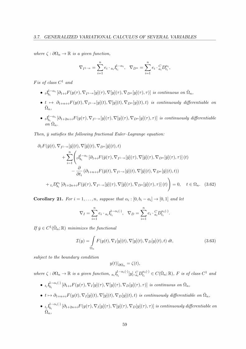
3.7. GENERALIZED VARIATIONAL CALCULUS OF SEVERAL VARIABLES
where ζ : ∂Ωn → R is a given function,
∇I1−α =n∑i=1
ei · aiI1−αiti
, ∇Dα =n∑i=1
ei · CaiDαiti,
F is of class C1 and
• tI1−αibi
[∂1+iF (y(τ),∇I1−α [y](τ),∇[y](τ),∇Dα [y](τ), τ)] is continuous on Ωn,
• t 7→ ∂1+n+iF (y(t),∇I1−α [y](t),∇[y](t),∇Dα [y](t), t) is continuously differentiable onΩn,
• tI1−αibi
[∂1+2n+iF (y(τ),∇I1−α [y](τ),∇[y](τ),∇Dα [y](τ), τ)] is continuously differentiable
on Ωn.
Then, y satisfies the following fractional Euler–Lagrange equation:
∂1F (y(t),∇I1−α [y](t),∇[y](t),∇Dα [y](t), t)
+
n∑i=1
(tI
1−αibi
[∂1+iF (y(τ),∇I1−α [y](τ),∇[y](τ),∇Dα [y](τ), τ)] (t)
− ∂
∂ti(∂1+n+iF (y(t),∇I1−α [y](t),∇[y](t),∇Dα [y](t), t))
+ tiDαibi
[∂1+2n+iF (y(τ),∇I1−α [y](τ),∇[y](τ),∇Dα [y](τ), τ)] (t)
)= 0, t ∈ Ωn. (3.62)
Corollary 21. For i = 1, . . . , n, suppose that αi : [0, bi − ai]→ [0, 1] and let
∇I =
n∑i=1
ei · aiI1−αi(·)ti
, ∇D =
n∑i=1
ei · CaiDαi(·)ti
.
If y ∈ C1(Ωn;R) minimizes the functional
I(y) =
∫Ωn
F (y(t),∇I [y](t),∇[y](t),∇D[y](t), t) dt, (3.63)
subject to the boundary condition
y(t)|∂Ωn= ζ(t),
where ζ : ∂Ωn → R is a given function, aiI1−αi(·)ti
[y], CaiDαi(·)ti∈ C(Ωn;R), F is of class C1 and
• tiI1−αi(·)bi
[∂1+iF (y(τ),∇I [y](τ),∇[y](τ),∇D[y](τ), τ)] is continuous on Ωn,
• t 7→ ∂1+n+iF (y(t),∇I [y](t),∇[y](t),∇D[y](t), t) is continuously differentiable on Ωn,
• tiI1−αi(·)bi
[∂1+2n+iF (y(τ),∇I [y](τ),∇[y](τ),∇D[y](τ), τ)] is continuously differentiable on
Ωn,
59

CHAPTER 3. STANDARD METHODS IN FRACTIONAL VARIATIONAL CALCULUS
then y satisfies the following equation
∂1F (y(t),∇I [y](t),∇[y](t),∇D[y](t), t)
+n∑i=1
(tiI
1−αi(·)bi
[∂1+iF (y(τ),∇I [y](τ),∇[y](τ),∇D[y](τ), τ)] (t)
− ∂
∂ti(∂1+n+iF (y(t),∇I [y](t),∇[y](t),∇D[y](t), t))
+ tiDαi(·)bi
[∂1+2n+iF (y(τ),∇I [y](τ),∇[y](τ),∇D[y](τ), τ)] (t)
)= 0, t ∈ Ωn. (3.64)
Theorem 13. Suppose that y ∈ A(ζ) satisfies (3.57) and function (x1, x2, x3, x4)→ F (x1, x2, x3, x4, t)is convex for every t ∈ Ωn. Then, y is a minimizer of functional (3.56).
Proof. Let y ∈ A(ζ) be a function satisfying equation (3.57) and such that (x1, x2, x3, x4)→F (x1, x2, x3, x4, t) is convex for every t ∈ Ωn. Then, the following inequality holds:
I(y) ≥ I(y)
+
∫Ωn
(∂1F (y − y) +
n∑i=1
[∂1+iF ·KPi [y − y] + ∂1+n+iF
∂
∂ti[y − y] + ∂1+2n+iF ·BPi [y − y]
])dt,
where functions ∂iF are evaluated at (y,∇KP [y],∇[y],∇BP [y], t), for i = 1, . . . , 3n+ 1. More-over, using the classical integration by parts formula, as well as Theorem 10 and the fact thaty − y|∂Ωn
= 0, we obtain
I(y) ≥ I(y) +
∫Ωn
(∂1F +
n∑i=1
[KP ∗i
[∂1+iF ] +∂
∂ti(∂1+n+iF ) +AP ∗i [∂1+2n+iF ]
])(y − y) dt.
Finally, applying equation (3.57), we have I(y) ≥ I(y) for any y ∈ A(ζ) and the proof iscomplete.
3.7.3 Dirichlet’s Principle
One of the most important variational principles for PDEs is Dirichlet’s principle for theLaplace equation. We shall present its generalized fractional counterpart.
We show that the solution of the generalized fractional boundary value problemn∑i=1
AP ∗i [BPi [y]] = 0 in Ωn, (3.65)
y = ζ on ∂Ωn, (3.66)
can be characterized as a minimizer of the following variational functional
I(y) =
∫Ωn
|∇BP [y]|2 dt (3.67)
60
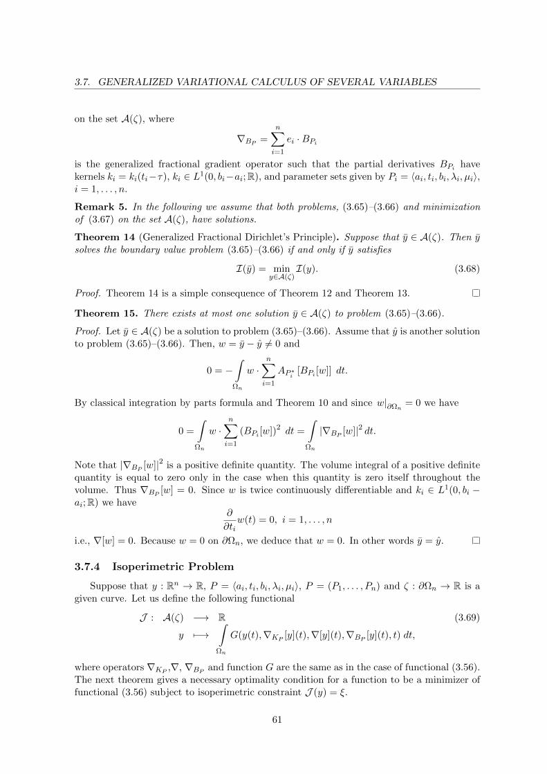
3.7. GENERALIZED VARIATIONAL CALCULUS OF SEVERAL VARIABLES
on the set A(ζ), where
∇BP =n∑i=1
ei ·BPi
is the generalized fractional gradient operator such that the partial derivatives BPi havekernels ki = ki(ti−τ), ki ∈ L1(0, bi−ai;R), and parameter sets given by Pi = 〈ai, ti, bi, λi, µi〉,i = 1, . . . , n.
Remark 5. In the following we assume that both problems, (3.65)–(3.66) and minimizationof (3.67) on the set A(ζ), have solutions.
Theorem 14 (Generalized Fractional Dirichlet’s Principle). Suppose that y ∈ A(ζ). Then ysolves the boundary value problem (3.65)–(3.66) if and only if y satisfies
I(y) = miny∈A(ζ)
I(y). (3.68)
Proof. Theorem 14 is a simple consequence of Theorem 12 and Theorem 13.
Theorem 15. There exists at most one solution y ∈ A(ζ) to problem (3.65)–(3.66).
Proof. Let y ∈ A(ζ) be a solution to problem (3.65)–(3.66). Assume that y is another solutionto problem (3.65)–(3.66). Then, w = y − y 6= 0 and
0 = −∫
Ωn
w ·n∑i=1
AP ∗i [BPi [w]] dt.
By classical integration by parts formula and Theorem 10 and since w|∂Ωn= 0 we have
0 =
∫Ωn
w ·n∑i=1
(BPi [w])2 dt =
∫Ωn
|∇BP [w]|2 dt.
Note that |∇BP [w]|2 is a positive definite quantity. The volume integral of a positive definitequantity is equal to zero only in the case when this quantity is zero itself throughout thevolume. Thus ∇BP [w] = 0. Since w is twice continuously differentiable and ki ∈ L1(0, bi −ai;R) we have
∂
∂tiw(t) = 0, i = 1, . . . , n
i.e., ∇[w] = 0. Because w = 0 on ∂Ωn, we deduce that w = 0. In other words y = y.
3.7.4 Isoperimetric Problem
Suppose that y : Rn → R, P = 〈ai, ti, bi, λi, µi〉, P = (P1, . . . , Pn) and ζ : ∂Ωn → R is agiven curve. Let us define the following functional
J : A(ζ) −→ R
y 7−→∫
Ωn
G(y(t),∇KP [y](t),∇[y](t),∇BP [y](t), t) dt,
(3.69)
where operators ∇KP ,∇, ∇BP and function G are the same as in the case of functional (3.56).The next theorem gives a necessary optimality condition for a function to be a minimizer offunctional (3.56) subject to isoperimetric constraint J (y) = ξ.
61
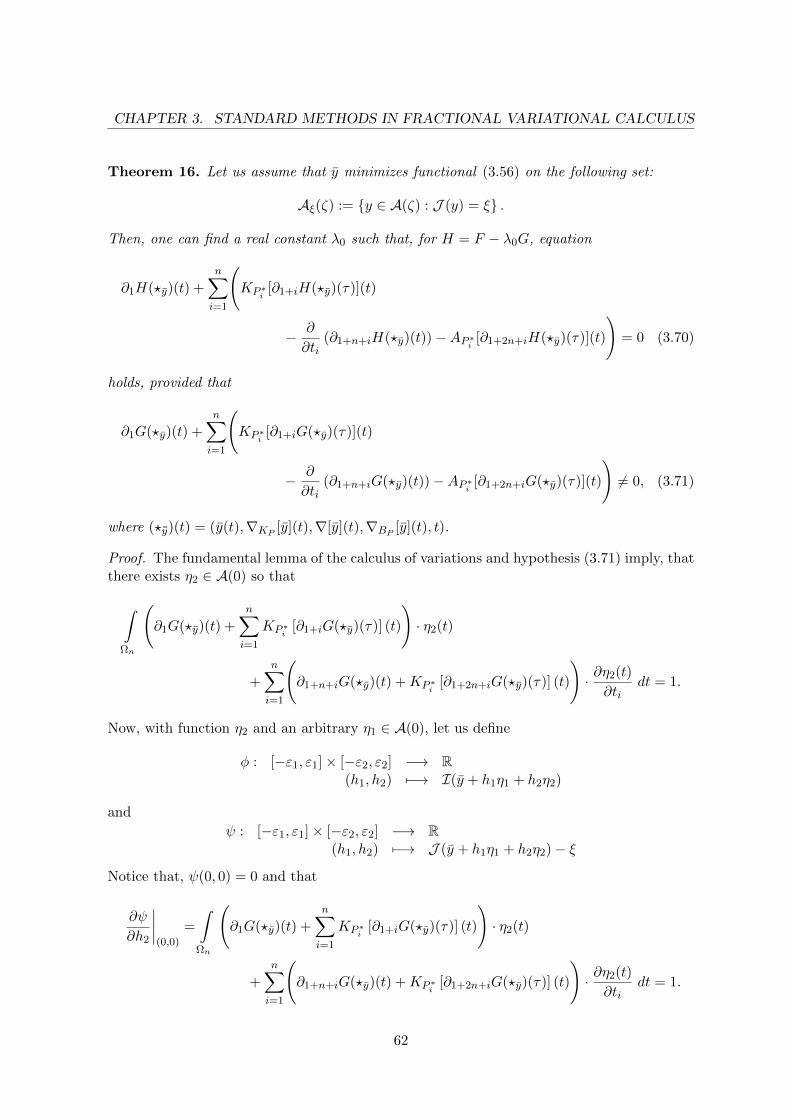
CHAPTER 3. STANDARD METHODS IN FRACTIONAL VARIATIONAL CALCULUS
Theorem 16. Let us assume that y minimizes functional (3.56) on the following set:
Aξ(ζ) := y ∈ A(ζ) : J (y) = ξ .
Then, one can find a real constant λ0 such that, for H = F − λ0G, equation
∂1H(?y)(t) +
n∑i=1
(KP ∗i
[∂1+iH(?y)(τ)](t)
− ∂
∂ti(∂1+n+iH(?y)(t))−AP ∗i [∂1+2n+iH(?y)(τ)](t)
)= 0 (3.70)
holds, provided that
∂1G(?y)(t) +
n∑i=1
(KP ∗i
[∂1+iG(?y)(τ)](t)
− ∂
∂ti(∂1+n+iG(?y)(t))−AP ∗i [∂1+2n+iG(?y)(τ)](t)
)6= 0, (3.71)
where (?¯y)(t) = (y(t),∇KP [y](t),∇[y](t),∇BP [y](t), t).
Proof. The fundamental lemma of the calculus of variations and hypothesis (3.71) imply, thatthere exists η2 ∈ A(0) so that
∫Ωn
(∂1G(?y)(t) +
n∑i=1
KP ∗i[∂1+iG(?y)(τ)] (t)
)· η2(t)
+
n∑i=1
(∂1+n+iG(?y)(t) +KP ∗i
[∂1+2n+iG(?y)(τ)] (t)
)· ∂η2(t)
∂tidt = 1.
Now, with function η2 and an arbitrary η1 ∈ A(0), let us define
φ : [−ε1, ε1]× [−ε2, ε2] −→ R(h1, h2) 7−→ I(y + h1η1 + h2η2)
and
ψ : [−ε1, ε1]× [−ε2, ε2] −→ R(h1, h2) 7−→ J (y + h1η1 + h2η2)− ξ
Notice that, ψ(0, 0) = 0 and that
∂ψ
∂h2
∣∣∣∣(0,0)
=
∫Ωn
(∂1G(?y)(t) +
n∑i=1
KP ∗i[∂1+iG(?y)(τ)] (t)
)· η2(t)
+
n∑i=1
(∂1+n+iG(?y)(t) +KP ∗i
[∂1+2n+iG(?y)(τ)] (t)
)· ∂η2(t)
∂tidt = 1.
62

3.7. GENERALIZED VARIATIONAL CALCULUS OF SEVERAL VARIABLES
The implicit function theorem implies, that there is ε0 > 0 and a function s ∈ C1([−ε0, ε0];R)with s(0) = 0 such that
ψ(h1, s(h1)) = 0, |h1| ≤ ε0,
and then y + h1η1 + s(h1)η2 ∈ Aξ(ζ). Moreover,
∂ψ
∂h1+∂ψ
∂h2· s′(h1) = 0, |h1| ≤ ε0,
and then
s′(0) = − ∂ψ∂h1
∣∣∣∣(0,0)
.
Because y ∈ A(ζ) is a minimizer of I we have
φ(0, 0) ≤ φ(h1, s(h1)), |h1| ≤ ε0,
and hence∂φ
∂h1
∣∣∣∣(0,0)
+∂φ
∂h2
∣∣∣∣(0,0)
· s′(0) = 0.
Letting λ0 = ∂φ∂h2
∣∣∣(0,0)
be the Lagrange multiplier we find
∂φ
∂h1
∣∣∣∣(0,0)
− λ0∂ψ
∂h1
∣∣∣∣(0,0)
= 0
or, in other words,
∫Ωn
[(∂1F (?y)(t) +
n∑i=1
KP ∗i[∂1+iF (?y)(τ)] (t)
)· η1(t)
+
n∑i=1
(∂1+n+iF (?y)(t) +KP ∗i
[∂1+2n+iF (?y)(τ)] (t)
)· ∂η1(t)
∂ti
]
− λ0
[(∂1G(?y)(t) +
n∑i=1
KP ∗i[∂1+iG(?y)(τ)] (t)
)· η1(t)
+n∑i=1
(∂1+n+iG(?y)(t) +KP ∗i
[∂1+2n+iG(?y)(τ)] (t)
)· ∂η1(t)
∂ti
]dt = 0.
Finally, applying the integration by parts formula for classical and fractional derivatives, andby the fundamental lemma of the calculus of variations we obtain (3.70).
Corollary 22. Let us assume that α = (α1, . . . , αn) ∈ (0, 1)n and y ∈ C1(Ωn;R) is minimizerof functional (3.60) subject to the isoperimetric constraint J (y) = ξ, where
J (y) =
∫Ωn
G(y(t),∇I1−α [y](t),∇[y](t),∇Dα [y](t), t) dt (3.72)
and boundary condition (3.61). Moreover
63
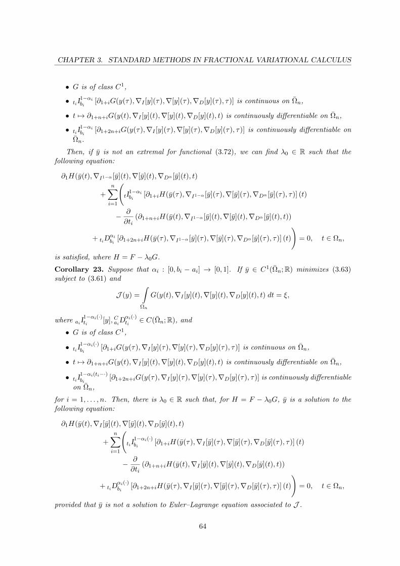
CHAPTER 3. STANDARD METHODS IN FRACTIONAL VARIATIONAL CALCULUS
• G is of class C1,
• tiI1−αibi
[∂1+iG(y(τ),∇I [y](τ),∇[y](τ),∇D[y](τ), τ)] is continuous on Ωn,
• t 7→ ∂1+n+iG(y(t),∇I [y](t),∇[y](t),∇D[y](t), t) is continuously differentiable on Ωn,
• tiI1−αibi
[∂1+2n+iG(y(τ),∇I [y](τ),∇[y](τ),∇D[y](τ), τ)] is continuously differentiable on
Ωn.
Then, if y is not an extremal for functional (3.72), we can find λ0 ∈ R such that thefollowing equation:
∂1H(y(t),∇I1−α [y](t),∇[y](t),∇Dα [y](t), t)
+n∑i=1
(tI
1−αibi
[∂1+iH(y(τ),∇I1−α [y](τ),∇[y](τ),∇Dα [y](τ), τ)] (t)
− ∂
∂ti(∂1+n+iH(y(t),∇I1−α [y](t),∇[y](t),∇Dα [y](t), t))
+ tiDαibi
[∂1+2n+iH(y(τ),∇I1−α [y](τ),∇[y](τ),∇Dα [y](τ), τ)] (t)
)= 0, t ∈ Ωn,
is satisfied, where H = F − λ0G.
Corollary 23. Suppose that αi : [0, bi − ai] → [0, 1]. If y ∈ C1(Ωn;R) minimizes (3.63)subject to (3.61) and
J (y) =
∫Ωn
G(y(t),∇I [y](t),∇[y](t),∇D[y](t), t) dt = ξ,
where aiI1−αi(·)ti
[y], CaiDαi(·)ti∈ C(Ωn;R), and
• G is of class C1,
• tiI1−αi(·)bi
[∂1+iG(y(τ),∇I [y](τ),∇[y](τ),∇D[y](τ), τ)] is continuous on Ωn,
• t 7→ ∂1+n+iG(y(t),∇I [y](t),∇[y](t),∇D[y](t), t) is continuously differentiable on Ωn,
• tiI1−αi(ti−·)bi
[∂1+2n+iG(y(τ),∇I [y](τ),∇[y](τ),∇D[y](τ), τ)] is continuously differentiable
on Ωn,
for i = 1, . . . , n. Then, there is λ0 ∈ R such that, for H = F − λ0G, y is a solution to thefollowing equation:
∂1H(y(t),∇I [y](t),∇[y](t),∇D[y](t), t)
+n∑i=1
(tiI
1−αi(·)bi
[∂1+iH(y(τ),∇I [y](τ),∇[y](τ),∇D[y](τ), τ)] (t)
− ∂
∂ti(∂1+n+iH(y(t),∇I [y](t),∇[y](t),∇D[y](t), t))
+ tiDαi(·)bi
[∂1+2n+iH(y(τ),∇I [y](τ),∇[y](τ),∇D[y](τ), τ)] (t)
)= 0, t ∈ Ωn,
provided that y is not a solution to Euler–Lagrange equation associated to J .
64
3.7. GENERALIZED VARIATIONAL CALCULUS OF SEVERAL VARIABLES
3.7.5 Noether’s Theorem
In Section 3.5 of this thesis, we have proved a generalized fractional version of Noether’stheorem. That is, assuming invariance of Lagrangian under changes in the coordinate system,we showed that its extremal must satisfy equation (3.43). In this section, we prove a gener-alized multidimensional fractional Noether’s theorem. As before, we start with definitions ofextremal and invariance.
Definition 26. A function y ∈ C1(Ωn;R) such that KPi [y], BPi [y] ∈ C(Ωn;R), i = 1, . . . , nsatisfying equation (3.57) is said to be a generalized fractional extremal.
We consider a one–parameter family of transformations of the form y(t) = φ(θ, t, y(t)),where φ is a map of class C2:
φ : [−ε, ε]× Ωn × R −→ R(θ, t, x) 7−→ φ(θ, t, x),
such that φ(0, t, x) = x. Note that, using Taylor’s expansion of φ(θ, t, y(t)) in a neighborhoodof 0 one has
y(t) = φ(0, t, y(t)) + θ∂
∂θφ(0, t, y(t)) + o(θ),
provided that θ ∈ [−ε, ε]. Moreover, having in mind that φ(0, t, y(t)) = y(t) and denotingξ(t, y(t)) = ∂
∂θφ(0, t, y(t)), one has
y(t) = y(t) + θξ(t, y(t)) + o(θ), (3.73)
so that, for θ ∈ [−ε, ε] the linear approximation to the transformation is
y(t) ≈ y(t) + θξ(t, y(t)).
Now, let us introduce the notion of invariance.
Definition 27. We say that the Lagrangian F is invariant under the one–parameter familyof infinitesimal transformations (3.73), where ξ is such that t 7→ ξ(t, y(t)) ∈ C1
(Ωn;R
)with
KPi [τ 7→ ξ(τ, y(τ))] , BPi [τ 7→ ξ(τ, y(τ))] ∈ C(Ωn;R
), i = 1, . . . , n, if
F (y(t),∇KP [y](t),∇[y](t),∇BP [y](t), t) = F (y(t),∇KP [y](t),∇[y](t),∇BP [y](t), t), (3.74)
for all θ ∈ [−ε, ε], and all y ∈ C1(Ωn;R
)with KPi [y], BPi [y] ∈ C
(Ωn;R
), i = 1, . . . , n.
Similarly to Section 3.5, we want to state Noether’s theorem in a compact form. For thatwe introduce the following two bilinear operators:
Di[f, g] := f ·AP ∗i [g] + g ·BPi [f ], (3.75)
Ii[f, g] := −f ·KP ∗i[g] + g ·KPi [f ], (3.76)
where i = 1, . . . , n.
Now we are ready to state the generalized fractional Noether’s theorem.
65

CHAPTER 3. STANDARD METHODS IN FRACTIONAL VARIATIONAL CALCULUS
Theorem 17 (Generalized Multidimensional Fractional Noether’s Theorem). Let F be in-variant under the one–parameter family of infinitesimal transformations (3.73). Then forevery generalized fractional extremal the following equality holds
n∑i=1
Ii [ξ(t, y(t)), ∂1+iF (?y)(t)] +∂
∂ti(ξ(t, y(t)) · ∂1+n+iF (?y)(t))
+ Di [ξ(t, y(t)), ∂1+2n+iF (?y)(t)] = 0, t ∈ Ωn, (3.77)
where (?y)(t) = (y(t),∇KP [y](t),∇[y](t),∇BP [y](t), t).
Proof. By equation (3.74) one has
d
dθ[F (y(t),∇KP [y](t),∇[y](t),∇BP [y](t), t)]
∣∣∣∣θ=0
= 0
The usual chain rule implies
∂1F (?y)(t) ·d
dθy(t) +
n∑i=1
∂1+iF (?y)(t) ·d
dθKPi [y](t)
+ ∂1+n+iF (?y)(t) ·d
dθ
∂
∂tiy(t) + ∂1+2n+iF (?y)(t) ·
d
dθBPi [y](t)
∣∣∣∣∣θ=0
= 0.
By linearity of KPi , BPi , i = 1, . . . , n differentiating with respect to θ, and putting θ = 0 wehave
∂1F (?y)(t) · ξ(t, y(t)) +n∑i=1
∂1+iF (?y)(t) ·KPi [τ 7→ ξ(τ, y(τ))](t)
+ ∂1+n+iF (?y)(t) ·∂
∂tiξ(t, y(t)) + ∂1+2n+iF (?y)(t) ·BPi [τ 7→ ξ(τ, y(τ))](t) = 0.
Now, using generalized Euler–Lagrange equation (3.57) and formulas (3.75) and (3.76) wearrive to (3.77).
Example 20. Let c ∈ R, P = (P1, . . . , Pn) with Pi = 〈ai, ti, bi, λi, µi〉 and y ∈ C1(Ωn;R)with BPi [y] ∈ C(Ωn;R), i = 1, . . . , n. We consider one–parameter family of infinitesimaltransformations
y(t) = y(t) + εc+ o(ε), (3.78)
and the Lagrangian F (∇BP [y](t), t) Then we have
F (∇BP [y](t), t) = F (∇BP [y](t), t) .
Hence, F is invariant under (3.78) and Theorem 17 asserts that
n∑i=1
Di [c, ∂n+iF (∇BP [y](t), t)] = 0. (3.79)
Similarly to the previous sections, one can obtain from Theorem 17 results regarding toconstant and variable order fractional integrals and derivatives.
66
3.8. CONCLUSION
Corollary 24. Suppose that α = (α1, . . . , αn) ∈ (0, 1)n and that
F (y(t),∇I1−α [y](t),∇[y](t),∇Dα [y](t), t) = F (y(t),∇I1−α [y](t),∇[y](t),∇Dα [y](t), t),
where y ∈ C1(Ωn;R) and y is the family (3.73). Then all solutions of the Euler–Lagrangeequation (3.62) satisfy
n∑i=1
I1−αii [ξ, ∂1+iF ] +
∂
∂ti(ξ · ∂1+n+iF ) + Dαi
i [ξ, ∂1+2n+iF ] = 0,
whereDαii [f, g] := −f · tiD
αibi
[g] + g · CaiDαiti
[f ],
I1−αii [f, g] := −f · tI1−αibi
[g] + g · aiI1−αiti
[f ], i = 1, . . . , n,
function ξ is taken in (t, y(t)) and functions ∂jF are evaluated at (y(t),∇I1−α [y](t),∇[y](t),∇Dα [y](t), t)for j = 1, . . . , 3n.
Corollary 25. Let us assume that y ∈ C1(Ωn;R) with aiI1−αi(·)ti
[y], CaiD
αi(·)ti
[y] ∈ C(Ωn;R),αi : [0, bi − ai]→ [0, 1], and that
F (y(t),∇I [y](t),∇[y](t),∇D[y](t), t) = F (y(t),∇I [y](t),∇[y](t),∇D[y](t), t),
where y is the family (3.73) such that t 7→ ξ(t, y(t)) ∈ C1(Ωn;R) with aiI1−αi(·)ti
[τ 7→ ξ(τ, y(τ))],CaiD
αi(·)ti
[τ 7→ ξ(τ, y(τ))] ∈ C(Ωn;R). Then
n∑i=1
I1−αi(·,·)i [ξ, ∂1+iF ] +
∂
∂ti(ξ · ∂1+n+iF ) + D
αi(·,·)i [ξ, ∂1+2n+iF ] = 0,
along any solution of Euler–Lagrange equation (3.64), where
Dαi(·,·)i [f, g] := −f · tiD
αi(·,·)bi
[g] + g · CaiDαi(·,·)ti
[f ],
I1−αi(·,·)i [f, g] := −f · tiI
1−αi(·,·)bi
[g] + g · aiI1−αi(·,·)ti
[f ], i = 1, . . . , n,
function ξ is taken in (t, y(t)) and functions ∂jF are evaluated at (y(t),∇I [y](t),∇[y](t),∇D[y](t), t)for j = 1, . . . , 3n.
3.8 Conclusion
In this chapter we unified, subsumed and significantly extended the necessary optimalityconditions available in the literature of the fractional calculus of variations. It should be men-tioned, however, that since fractional operators are nonlocal, it can be extremely challengingto find analytical solutions to fractional problems of the calculus of variations and, in manycases, solutions may not exist. Here, we gave several examples with analytic solutions, andmany more can be found borrowing different kernels from the book [92]. On the other hand,one can easily choose examples for which the fractional Euler–Lagrange differential equationsare hard to solve, and in that case one needs to use numerical methods [10]. However, inthe absence of existence, the necessary conditions for extremality are vacuous: one can not
67

CHAPTER 3. STANDARD METHODS IN FRACTIONAL VARIATIONAL CALCULUS
characterize an entity that does not exist in the first place. For solving a problem of thefractional calculus of variations one should proceed along the following three steps: (i) first,prove that a solution to the problem exists; (ii) second, verify the applicability of necessaryoptimality conditions; (iii) finally, apply the necessary conditions which identify the extremals(the candidates). Further elimination, if necessary, identifies the minimizer(s) of the problem.All three steps in the above procedure are crucial. As mentioned by Young in [106], thecalculus of variations has born from the study of necessary optimality conditions, but anysuch theory is ”naive” until the existence of minimizers is verified. Therefore, in the nextchapter, we shall follow the direct approach, first proving that a solution exists and nextfinding candidates with the help of the necessary optimality conditions.
3.9 State of the Art
The results of this chapter were published in [75,77–83,86,87] and were presented by theauthor at several international conferences:
• International Mathematical Symposium on Mathematical Theory of Networks and Sys-tems, 9th July– 13th July 2012, Melbourne, Australia. Presentation: A GeneralizedFractional Calculus with Applications [84]. Talk at invited session.
• 5th Symposium on Fractional Differentiation and Its Applications, 14th May– 17th May2012, Nanjing, China. Presentation: Generalized Fractional Green’s Theorem. Talk atinvited session.
• Transform methods and special functions, 20th October– 23rd October 2011, Sofia,Bulgaria. Presentation: Fractional Variational Calculus of Variable Order.
• SIAM Conference on Control and Its Applications, 8th July– 12th July 2011, Baltimore,United States of America. Presentation: Fractional Variational Calculus with Classicaland Combined Caputo Derivatives. Talk at invited session.
• International Conference on Isoperimetric Problem of Queen Dido and its MathematicalRamifications, 24th May– 29th May 2010, Tunis, Tunisia. Presentation: FractionalIsoperimetric Problems.
• Workshop on Variational Analysis and Applications, October 2011, Evora, Portugal.Presentation: Fractional Variational Calculus with Classical and Combined CaputoDerivatives.
• The 4th IFAC Workshop on Fractional Differentiation and its Applications, 18th October–20th October 2010, Badajoz, Spain. Presentation: Calculus of Variations with Frac-tional and Classical Derivatives [76].
• 8th EUROPT Workshop on Advances in Continuous Optimization, 9th July– 10th July2010, Aveiro, Portugal. Presentation: Necessary Optimality Conditions for FractionalVariational Problem.
Paper [87] entitled Green’s theorem for generalized fractional derivatives [85] received theGrunvald-Letnikov Award, Best Student Paper (Theory) at the conference ’Fractional Differ-entiation and its Applications’ in May 2012, Nanjing, China. More detailed information canbe found at http://em.hhu.edu.cn/fda12/Awards.html.
68
Chapter 4
Direct Methods in FractionalCalculus of Variations
In this chapter we study the fundamental problem of calculus of variations with a La-grangian depending on generalized fractional integrals and generalized fractional derivatives.In contrast with the standard approach presented in Chapter 3, we use direct methods toaddress the problem of finding minima to generalized fractional functionals. First, we proveexistence of solutions in an appropriate space of functions and under suitable assumptionsof regularity, coercivity and convexity. Next, we proceed with application of an optimalitycondition, and finish examining the candidates to arrive to solution.
Let us briefly describe the main contents of the chapter. In Section 4.1 we prove a Tonellitype theorem ensuring existence of minimizers for generalized fractional functionals. We alsogive sufficient conditions for a regular Lagrangian and for a coercive functional. Section 4.2 isdevoted to a necessary optimality condition for minimizers. In the last Section 4.3 we improveour results assuming more regularity of the Lagrangian and generalized fractional operators.
4.1 Existence of a Minimizer for a Generalized Functional
Let us recall that 1 < p, q <∞ and 1p + 1
q = 1. In this section, our aim is to give sufficientconditions ensuring the existence of a minimizer for the following generalized Lagrangianfunctional:
I : A −→ R
y 7−→b∫aF (y(t),KP [y](t), y(t), BP [y](t), t) dt,
where A is a weakly closed subset of W 1,p(a, b;R), y denotes the derivative of y, KP is thegeneralized fractional integral with a kernel in Lq(∆;R), BP = d
dt KP is the generalizedfractional Caputo derivative, P = 〈a, t, b, λ, µ〉 is a set of parameters and F is a Lagrangianof class C1:
F : R4 × [a, b] −→ R(x1, x2, x3, x4, t) 7−→ F (x1, x2, x3, x4, t).
69

CHAPTER 4. DIRECT METHODS IN FRACTIONAL CALCULUS OF VARIATIONS
4.1.1 A Tonelli-type Theorem
In this section we state a Tonelli-type theorem ensuring the existence of a minimizer forI with the help of general assumptions of regularity, coercivity and convexity. These threehypothesis are usual in the classical case, see [33]. Precisely:
Definition 28. A Lagrangian F is said to be regular if it satisfies:
• t 7→ F (y(t),KP [y](t), y(t), BP [y](t), t) ∈ L1(a, b;R);
• t 7→ ∂1F (y(t),KP [y](t), y(t), BP [y](t), t) ∈ L1(a, b;R);
• t 7→ ∂2F (y(t),KP [y](t), y(t), BP [y](t), t) ∈ Lp(a, b;R);
• t 7→ ∂3F (y(t),KP [y](t), y(t), BP [y](t), t) ∈ Lq(a, b;R);
• t 7→ ∂4F (y(t),KP [y](t), y(t), BP [y](t), t) ∈ Lp(a, b;R),
for any y ∈W 1,p(a, b;R):
Definition 29. Functional I is said to be coercive on A if it satisfies:
lim‖y‖W1,p→∞
y∈A
I(y) = +∞.
We are now in position to state the following result:
Theorem 18 (Tonelli-type Theorem). Let us assume that:
• F is regular;
• I is coercive on A;
• F (·, t) is convex on (Rd)4 for any t ∈ [a, b].
Then, there exists a minimizer for I.
Proof. Since F is regular, for any y ∈ A, t 7→ F (y(t),KP [y](t), y(t), BP [y](t), t) ∈ L1(a, b;R)and then I(y) exists in R. Let us introduce a minimizing sequence (yn)n∈N ⊂ A satisfying:
I(yn) −→ infy∈AI(y) < +∞.
Since I is coercive, (yn)n∈N is bounded in W 1,p(a, b;R). Since W 1,p(a, b;R) is a reflexiveBanach space, it exists a subsequence of (yn)n∈N weakly convergent in W 1,p(a, b;R). In thefollowing, we still denote this subsequence by (yn)n∈N and we denote by y its weak limit.Since A is a weakly closed subset of W 1,p(a, b;R), y ∈ A. Finally, using the convexity of F ,we have for any n ∈ N:
I(yn) ≥ I(y) +
b∫a
∂1F · (yn(t)− y(t)) + ∂2F · (KP [yn](t)−KP [y](t))
+ ∂3F · (yn(t)− ˙y(t)) + ∂4F · (BP [yn](t)−BP [y](t)) dt, (4.1)
where ∂iF are taken in (y(t),KP [y](t), ˙y(t), BP [y](t), t) for any i = 1, 2, 3, 4.
Now, from these four following facts:
70

4.1. EXISTENCE OF A MINIMIZER FOR A GENERALIZED FUNCTIONAL
• F is regular;
• ynW 1,p
−−− y;
• KP is linear bounded from Lp(a, b;R) to Lq(a, b;R);
• the compact embedding W 1,p(a, b;R) C([a, b];R) holds;
one can easily conclude that:
• t 7→ ∂3F (y(t),KP [y](t), ˙y(t), BP [y](t), t) ∈ Lq(a, b;R) and ynLp− ˙y;
• t 7→ ∂4F (y(t),KP [y](t), ˙y(t), BP [y](t), t) ∈ Lp(a, b;R) and BP [yn]Lq− BP [y];
• t 7→ ∂1F (y(t),KP [y](t), ˙y(t), BP [y](t), t) ∈ L1(a, b;R) and ynL∞−−→ y;
• t 7→ ∂2F (y(t),KP [y](t), ˙y(t), BP [y](t), t) ∈ Lp(a, b;R) and KP [yn]Lq−→ K[y].
Finally, when n tends to ∞ in the inequality (4.1), we obtain:
infy∈AI(y) ≥ I(y) ∈ R,
which completes the proof.
The first two hypothesis of Theorem 18 are very general. Consequently, in Sections 4.1.2and 4.1.3, we give concrete assumptions on F ensuring its regularity and the coercivity of I.
The last hypothesis of convexity is strong. Nevertheless, from more regularity assumptionson F , on KP and on BP , we prove in Section 4.3 that we can provide versions of Theorem 18with weaker convexity assumptions.
4.1.2 Sufficient Condition for a Regular Lagrangians
In this Section, we give a sufficient condition on F implying its regularity. First, for anyM ≥ 1, let us define the set PM of maps P such that for any (x1, x2, x3, x4, t) ∈ (R)4× [a, b]:
P (x1, x2, x3, x4, t) =
N∑k=0
ck(x1, t) |x2|d2,k |x3|d3,k |x4|d4,k ,
with N ∈ N and where, for any k = 0, . . . , N , ck : R× [a, b] −→ R+ is continuous and(d2,k, d3,k, d4,k) ∈ [0, q]× [0, p]× [0, q] satisfies d2,k + (q/p)d3,k + d4,k ≤ (q/M).
The following lemma shows the interest of sets PM .
Lemma 1. Let M ≥ 1 and P ∈PM . Then:
∀y ∈W 1,p(a, b;R), t 7→ P (y(t),KP [y](t), y(t), BP [y](t), t) ∈ LM (a, b;R).
Proof. For any k = 0, . . . , N , ck(u, t) is continuous and then it is in L∞(a, b;R). We alsohave |KP [y]|d2,k ∈ Lq/d2,k(a, b;R), |y|d3,k ∈ Lp/d3,k(a, b;R) and |BP [y]|d4,k ∈ Lq/d4,k(a, b;R).Consequently:
ck(u, t) |KP [y]|d2,k |y|d3,k |BP [y]|d4,k ∈ Lr(a, b;R), (4.2)
with r = q/(d2,k + (q/p)d3,k + d4,k) ≥M . The proof is complete.
71

CHAPTER 4. DIRECT METHODS IN FRACTIONAL CALCULUS OF VARIATIONS
Then, from this previous Lemma, one can easily obtain the following proposition.
Proposition 1. Let us assume that there exist P0 ∈ P1, P1 ∈ P1, P2 ∈ Pp, P3 ∈ Pq andP4 ∈Pp such that for any (x1, x2, x3, x4, t) ∈ (R)4 × [a, b]:
• |F (x1, x2, x3, x4, t)| ≤ P0(x1, x2, x3, x4, t);
• |∂1F (x1, x2, x3, x4, t)| ≤ P1(x1, x2, x3, x4, t);
• |∂2F (x1, x2, x3, x4, t)| ≤ P2(x1, x2, x3, x4, t);
• |∂3F (x1, x2, x3, x4, t)| ≤ P3(x1, x2, x3, x4, t);
• |∂4F (x1, x2, x3, x4, t)| ≤ P4(x1, x2, x3, x4, t).
Then, F is regular.
This last proposition states that if the norms of F and of its partial derivatives arecontrolled from above by elements of PM , then F is regular. We will see some examplesin Section 4.1.4.
4.1.3 Sufficient Condition for a Coercive Functionals
The definition of coercivity for functional I is strongly dependent on the considered setA. Consequently, in this section, we will consider an example of set A and we will give asufficient condition on F ensuring the coercivity of I in this case.
Precisely, let us consider ya ∈ R and A = W 1,pa (a, b;R) where W 1,p
a (a, b;R) := y ∈W 1,p(a, b;R), y(a) = ya. From the compact embeddingW 1,p(a, b;R) C([a, b];R), W 1,p
a (a, b;R)is weakly closed in W 1,p(a, b;R).
An important consequence of such a choice of set A is given by the following lemma.
Lemma 2. There exist A0, A1 ≥ 0 such that for any y ∈W 1,pa (a, b;R):
• ‖y‖L∞ ≤ A0 ‖y‖Lp +A1;
• ‖KP [y]‖Lq ≤ A0 ‖y‖Lp +A1;
• ‖BP [y]‖Lq ≤ A0 ‖y‖Lp +A1.
Proof. The last inequality comes from the boundedness of KP . Let us consider the second one.For any y ∈W 1,p
a (a, b;R), we have ‖y‖Lp ≤ ‖y − ya‖Lp+‖ya‖Lp ≤ (b−a) ‖y‖Lp+(b−a)1/p |ya|.We conclude using again the boundedness of KP . Now, let us consider the first inequality. Forany y ∈W 1,p
a (a, b;R), we have ‖y‖L∞ ≤ ‖y − ya‖L∞ + |ya| ≤ ‖y‖L1 + |ya| ≤ (b−a)1/q ‖y‖Lp +|ya|. Finally, we have just to define A0 and A1 as the maxima of the appearing constants.The proof is complete.
Precisely, Lemma 2 states the affine domination of the term ‖y‖Lp on the terms ‖y‖L∞ ,
‖KP [y]‖Lq and ‖BP [y]‖Lq for any y ∈W 1,pa (a, b;R). This characteristic of W 1,p
a (a, b;R) leadsus to give the following sufficient condition for a coercive functional I.
72
4.1. EXISTENCE OF A MINIMIZER FOR A GENERALIZED FUNCTIONAL
Proposition 2. Let us assume that for any (x1, x2, x3, x4, t) ∈ R4 × [a, b]:
F (x1, x2, x3, x4, t) ≥ c0 |x3|p +
N∑k=1
ck |x1|d1,k |x2|d2,k |x3|d3,k |x4|d4,k ,
with c0 > 0 and N ∈ N and where, for any k = 1, . . . , N , ck ∈ R and (d1,k, d2,k, d3,k, d4,k) ∈R+ × [0, q]× [0, p]× [0, q] satisfies:
d2,k + (q/p)d3,k + d4,k ≤ q and 0 ≤ d1,k + d2,k + d3,k + d4,k < p.
Then, I is coercive on W 1,pa (a, b;R).
Proof. Let us define rk = q/(d2,k + d4,k + (q/p)d3,k) ≥ 1 and let r′k denote the adjoint of rki.e., r′k = rk
rk−1. Using Holder’s inequality, one can easily prove that, for any y ∈W 1,p
a (a, b;R),
we have:
I(y) ≥ c0 ‖y‖Lp − (b− a)1/r′N∑k=1
|ck| ‖y‖d1,kL∞ ‖KP [y]‖d2,kLq ‖y‖
d3,kLp ‖BP [y]‖d4,kLq .
From the ”affine domination” of the term ‖y‖Lp on the terms ‖y‖L∞ , ‖KP [y]‖Lq and ‖BP [y]‖Lqfor any y ∈W 1,p
a (a, b;R) (see Lemma 2) and from the assumption 0 ≤ d1,k+d2,k+d3,k+d4,k <p, we obtain that:
lim‖y‖Lp→∞
y∈W 1,pa (a,b;R)
I(y) = +∞.
Finally, from Lemma 2, we also have in W 1,pa (a, b;R):
‖y‖Lp →∞⇐⇒ ‖y‖W 1,p →∞.
Consequently, I is coercive on W 1,pa (a, b;R). The proof is complete.
In this section, we have studied the case whereA is the weakly closed subset ofW 1,p(a, b;R)satisfying the initial condition y(a) = ya. For other examples of set A, let us note that allthe results of this section are still valid when:
• A is weakly closed subset of W 1,p(a, b;R) satisfying a final condition in t = b;
• A is weakly closed subset of W 1,p(a, b;R) satisfying two boundary conditions in t = aand in t = b.
4.1.4 Examples of Lagrangians
In this section, we give several examples of a convex Lagrangian F satisfying assumptionsof Propositions 1 and 2. In consequence, they are examples of application of Theorem 18 inthe case A = W 1,p
a (a, b;R).
Example 21. The most classical examples of a Lagrangian are the quadratic ones. Let usconsider the following:
F (x1, x2, x3, x4, t) = c(t) +1
2
4∑i=1
|xi|2 ,
73
CHAPTER 4. DIRECT METHODS IN FRACTIONAL CALCULUS OF VARIATIONS
where c : [a, b] → R is of class C1. One can easily check that F satisfies the assumptionsof Propositions 1 and 2 with p = q = 2. Moreover, F satisfies the convexity hypothesis ofTheorem 18. Consequently, one can conclude that there exists a minimizer of I defined onW 1,2a (a, b;R).
Example 22. Let us consider p = q = 2 and let us still denote by F the Lagrangian definedin Example 21. To obtain a more general example, one can define a Lagrangian F1 from Fas a time-dependent homothetic transformation and/or translation of its variables. Precisely:
F1(x1, x2, x3, x4, t) = F (c1(t)x1 +c01(t), c2(t)x2 +c0
2(t), c3(t)x3 +c03(t), c4(t)x4 +c0
4(t), t), (4.3)
where ci : [a, b] → R and c0i : [a, b] → R are of class C1 for any i = 1, 2, 3, 4. In this case,
F1 also satisfies convexity hypothesis of Theorem 18 and the assumptions of Proposition 1.Moreover, if c3 is with values in R+, then F1 also satisfies the assumptions of Proposition 2.
One should be careful: this last remark is not available in more general context. Precisely,if a general Lagrangian F satisfies the convexity hypothesis of Theorem 18 and assumptionsof Propositions 1 and 2, then Lagrangian F1 obtained by (4.3) also satisfies the convexityhypothesis of Theorem 18 and the assumptions of Proposition 1. Nevertheless, the assumptionof Proposition 2 can be lost by this process.
Example 23. We can also study quasi–linear examples given by Lagrangians of the type
F (x1, x2, x3, x4, t) = c(t) +1
p|x3|p +
4∑i=1
fi(t) · xi,
where c : [a, b] → R and for any i = 1, 2, 3, 4, fi : [a, b] → R are of class C1. In thiscase, F satisfies the assumptions of Propositions 1 and 2. Consequently, since F satisfiesthe convexity hypothesis of Theorem 18, one can conclude that there exists a minimizer of Idefined on W 1,p
a (a, b;R).
The most important constraint in order to apply Theorem 18 is the convexity hypothesis.This is the reason why the previous examples concern convex quasi–polynomial Lagrangians.Nevertheless, in Section 4.3, we are going to provide some improved versions of Theorem 18with weaker convexity assumptions. This will be allowed by more regularity hypotheses onF and/or on KP and BP . We refer to Section 4.3 for more details.
4.2 Necessary Optimality Condition for a Minimizer
In this section, we assume additionally that:
• F satisfies the assumptions of Proposition 1 (in particular, F is regular);
• A satisfies the following condition:
∀y ∈ A, ∀η ∈ C∞c , ∃0 < ε ≤ 1, ∀ |h| ≤ ε, y + hη ∈ A. (4.4)
74

4.2. NECESSARY OPTIMALITY CONDITION FOR A MINIMIZER
The assumption on A is satisfied if A + C∞c ⊂ A (for example A = W 1,pa (a, b;R) in Section
4.1.3). By C∞c we denote the space of infinitely differentiable functions compactly supportedin (a, b).
In the next theorem we will make use of the following Lemma.
Lemma 3. Let M ≥ 1 and P ∈ PM . Then, for any y ∈ A and any η ∈ C∞c , it existsg ∈ LM (a, b;R+) such that for any h ∈ [−ε, ε]:
P (y + hη,KP [y] + hKP [η], y + hη, BP [y] + hBP [η], t) ≤ g. (4.5)
Proof. Indeed, for any k = 0, . . . , N , for almost all t ∈ (a, b) and for any h ∈ [−ε, ε], we have:
ck(y(t) + hη(t), t) |KP [y](t) + hKP [η](t)|d2,k |y(t) + hη(t)|d3,k |BP [y](t) + hBP [η](t)|d4,k
≤ ck(|KP [y](t)|d2,k + |KP [η](t)|d2,k︸ ︷︷ ︸∈Lq/d2,k (a,b;R)
)(|y(t)|d3,k + |η(t)|d3,k︸ ︷︷ ︸∈Lp/d3,k (a,b;R)
)(|BP [y](t)|d4,k + |BP [η](t)|d4,k︸ ︷︷ ︸∈Lq/d4,k (a,b;R)
),
(4.6)
where ck = 2d2,k+d3,k+d4,k max[a,b]×[−ε,ε]
ck(y(t) + hη(t), t) exists in R because ck, y and η are
continuous. Since d2,k + (q/p)d3,k + d4,k ≤ (q/M), the right term in inequality (4.6) is inLM (a, b;R+) and is independent of h. The proof is completed.
Finally, from this previous Lemma, we can prove the following result:
Theorem 19. Let us assume that F satisfies assumptions of Proposition 1, I is coerciveand F (·, t) is convex on R4 for any t ∈ [a, b]. Then, the minimizer y ∈ A of I (given byTheorem 18) satisfies the generalized Euler-Lagrange equation
d
dt
(∂3F (?y)(t) +KP ∗ [∂4F (?y)(τ)](t)
)= ∂1F (?y)(t) +KP ∗ [∂2F (?y)(τ)](t), (GEL)
for almost all t ∈ (a, b), where (?y)(t) = (y(t),KP [y](t), ˙y(t), BP [y](t), t).
Proof. Since F satisfies the assumptions of Proposition 1, F is regular. Consequently, fromTheorem 18, we know that I admits a minimizer y ∈ A and then
I(y) ≤ I(y + hη), (4.7)
for any |h| ≤ ε and every η ∈ C∞c . Let us define the following map:
φy,η : [−ε, ε] −→ R
h 7−→ I(y + hη) =b∫aψy,η(t, h) dt,
where
ψy,η(t, h) := F (y(t) + hη(t),KP [y](t) + hKP [η](t), ˙y(t) + hη(t), BP [y](t) + hBP [η](t), t).
First we want to prove that the following term:
limh→0
I(y + hη)− I(y)
h= lim
h→0
φy,η(h)− φy,η(0)
h= φ′y,η(0) (4.8)
75
CHAPTER 4. DIRECT METHODS IN FRACTIONAL CALCULUS OF VARIATIONS
exists in R. In order to differentiate φy,η, we use the theorem of differentiation under theintegral sign. Indeed, we have for almost all t ∈ (a, b) that ψy,η(t, ·) is differentiable on [−ε, ε]with:
∀h ∈ [−ε, ε], ∂ψy,η∂h
(t, h)
= ∂1F (?y+hη)(t)·η(t)+∂2F (?y+hη)(t)·KP [η](t)+∂3F (?y+hη)(t)·η(t)+∂4F (?y+hη)(t)·BP [η](t).(4.9)
Since F satisfies the assumptions of Proposition 1, from Lemma 3 there exist g1 ∈ L1(a, b;R+),g2 ∈ Lp(a, b;R+), g3 ∈ Lq(a, b;R+) and g4 ∈ Lp(a, b;R+) such that for any h ∈ [−ε, ε] and foralmost all t ∈ (a, b):∣∣∣∣∂ψy,η∂h
(t, h)
∣∣∣∣ ≤ g1(t) |η(t)|+ g2(t) |KP [η](t)|+ g3(t) |η(t)|+ g4(t) |BP [η](t)| . (4.10)
Since η ∈ L∞(a, b;R), KP [η] ∈ Lq(a, b;R), η ∈ Lp(a, b;R) and BP [η] ∈ Lq(a, b;R), we canconclude that the right term in Inequality (4.10) is in L1(a, b;R+) and is independent of h.Consequently, we can use the theorem of differentiation under the integral sign and we obtainthat φy,η is differentiable with
∀h ∈ [−ε, ε], φ′y,η(h) =
b∫a
∂ψy,η∂h
(t, h) dt. (4.11)
Furthermore, inequality (4.7) implies
d
dhφy,η(h)
∣∣∣∣h=0
= 0,
what can be written as
b∫a
∂1F (?y)(t) · η(t) + ∂2F (?y)(t) ·KP [η](t) + ∂3F (?y)(t) · η(t) + ∂4F (?y)(t) ·BP [η](t) dt = 0.
Moreover, applying integration by parts formula (3.5) one has
b∫a
(∂1F (?y)(t) +KP ∗ [∂2F (?y)(τ)]
)· η(t) +
(∂3F (?y)(t) +KP ∗ [∂4F (?y)(τ)]
)· η(t) dt = 0.
Then, taking an absolutely continuous anti-derivative w of t 7→ ∂1F (?y)(t)+KP ∗ [∂2F (?y)(τ)](t) ∈L1(a, b;R), we obtain using integration by parts that:
b∫a
(∂3F (?y)(t) +KP ∗ [∂4F (?y)(τ)](t)− w(t)
)· η(t) dt = 0.
From the du Bois Reymond Lemma there exists a constant C ∈ R such that for almost allt ∈ (a, b), we have:
∂3F (?y)(t) +K∗[∂4F (?y)(τ)](t) = C + w(t). (4.12)
76
4.3. SOME IMPROVEMENTS
Since the right term is absolutely continuous, we can differentiate it almost everywhere on(a, b). Finally, we obtain that y is a critical point of I if and only if the following equationholds almost everywhere on (a, b):
d
dt
(∂3F (?y)(t) +KP ∗ [∂4F (?y)(τ)](t)
)= ∂1F (?y)(t) +KP ∗ [∂2F (?y)(τ)](t). (4.13)
The proof is completed.
We would like to remark that in the particular case, when kα(t, τ) = 1Γ(1−α)(t − τ)−α,
kα ∈ Lq(∆;R) and P = 〈a, t, b, 1, 0〉, then Sections 4.1.1, 4.1.2, 4.1.3, 4.1.4 and 4.2 recoverthe case of the following fractional variational functional
I : A −→ R
y 7−→b∫aF (y(t), aI
1−αt [y](t), y(t), Ca D
αt [y](t), t) dt,
studied in [23]. Moreover, if we choose the kernel kα(t, τ) = 1Γ(1−α(t,τ))(t − τ)−α(t,τ), kα ∈
Lq(∆;R) and the parameter set P = 〈a, t, b, 1, 0〉, then Sections 4.1.1, 4.1.2, 4.1.3, 4.1.4 and 4.2restore the case of the variable order fractional variational functional
I : A −→ R
y 7−→b∫aF(y(t), aI
1−α(·,·)t [y](t), y(t), Ca D
α(·,·)t [y](t), t
)dt.
4.3 Some Improvements
In this section, we assume more regularity of the Lagrangian F and of the operators KP
and BP . It allows to weaken the convexity assumption in Theorem 18 and/or the assumptionsof Propositions 1 and 2.
4.3.1 A First Weaker Convexity Assumption
Let us assume that F satisfies the following condition:
(F (·, x2, x3, x4, t))(x2,x3,x4,t)∈R3×[a,b] is uniformly equicontinuous on R. (4.14)
This condition has to be understood as:
∀ε > 0, ∃δ > 0,∀(u, v) ∈ R2, |u− v| ≤ δ =⇒ ∀(x2, x3, x4, t) ∈ R3 × [a, b],
|F (u, x2, x3, x4, t)− F (v, x2, x3, x4, t)| ≤ ε. (4.15)
For example, this condition is satisfied for a Lagrangian F with bounded ∂1F . In thiscase, we can prove the following improved version of Theorem 18:
Theorem 20. Let us assume that:
• F satisfies the condition given by (4.14);
• F is regular;
77

CHAPTER 4. DIRECT METHODS IN FRACTIONAL CALCULUS OF VARIATIONS
• I is coercive on A;
• L(x1, ·, t) is convex on R3 for any x1 ∈ R and for any t ∈ [a, b].
Then, there exists a minimizer for I.
Proof. Indeed, with the same proof of Theorem 18, we can construct a weakly convergentsequence (yn)n∈N ⊂ A satisfying
ynW 1,p
−−− y ∈ A and I(yn) −→ infy∈AI(y) < +∞.
Since the compact embedding W 1,p(a, b;R) C([a, b];R) holds, we have ynC→ y. Let ε > 0
and let us consider δ > 0 given by (4.15). There exists N ∈ N such that for any n ≥ N ,‖yn − y‖∞ ≤ δ. So, for any n ≥ N and for t ∈ (a, b):
|F (yn(t),KP [yn](t), yn(t), BP [yn](t), t)− F (y(t),KP [yn](t), yn(t), BP [yn](t), t)| ≤ ε.
Consequently, for any n ≥ N , we have
I(yn) ≥∫ b
aF (y(t),KP [yn](t), yn(t), BP [yn](t), t)dt− (b− a)ε.
From the convexity hypothesis and using the same strategy as in the proof of Theorem 18,we have by passing to the limit on n
infy∈AI(y) ≥ I(y)− (b− a)ε.
The proof is complete since the previous inequality is true for any ε > 0.
Such an improvement allows to give examples of a Lagrangian F without convexity on itsfirst variable. Taking inspiration from Example 21, we can provide the following example.
Example 24. Let us consider p = 2 and A = W 1,2a (a, b;R). Let us consider
F (x1, x2, x3, x4, t) = f(x1, t) +1
2
4∑i=2
|xi|2 ,
for any f : R × [a, b] → R of class C1 with ∂1f bounded (like sine and cosine functions). Inthis case, F satisfies the hypothesis of Theorem 20 and we can conclude with the existence ofa minimizer of I defined on A.
4.3.2 A Second Weaker Convexity Assumption
In this section, we assume that KP is moreover a linear bounded operator from C([a, b];R)to C([a, b];R). For example, this condition is satisfied by Riemann–Liouville fractional inte-grals (see [51,98] for detailed proofs). We also assume that F satisfies the following condition:
(F (·, ·, x3, x4, t))(x3,x4,t)∈R2×[a,b] is uniformly equicontinuous on R2. (4.16)
78

4.3. SOME IMPROVEMENTS
This condition has to be understood as:
∀ε > 0, ∃δ > 0,∀(u, v) ∈ R2,∀(u0, v0) ∈ R2 |u− v| ≤ δ, |u0 − v0| ≤ δ =⇒ ∀(x3, x4, t) ∈ R2×[a, b],
|F (u, u0, x3, x4, t)− F (v, v0, x3, x4, t)| ≤ ε. (4.17)
For example, this condition is satisfied for a Lagrangian F with bounded ∂1F and bounded∂2F . In this case, we can prove the following improved version of Theorem 18:
Theorem 21. Let us assume that:
• F satisfies the condition given by (4.16);
• F is regular;
• I is coercive on A;
• L(x1, x2, ·, t) is convex on R2 for any (x1, x2) ∈ R and for any t ∈ [a, b].
Then, there exists a minimizer for I.
Proof. Indeed, with the same proof of Theorem 18, we can construct a weakly convergentsequence (yn)n∈N ⊂ A satisfying
ynW 1,p
−−− y ∈ A and I(yn) −→ infy∈AI(y) < +∞.
Since the compact embedding W 1,p(a, b;R) C([a, b];R) holds, we have ynC→ y and since
KP is continuous from C([a, b];R) to C([a, b];R), we have KP [yn]C→ KP [y]. Let ε > 0 and let
us consider δ > 0 given by (4.17). There exists N ∈ N such that for any n ≥ N , ‖yn − y‖∞ ≤ δand ‖KP [yn]−KP [y]‖∞ ≤ δ. So, for any n ≥ N and for t ∈ (a, b):
|F (yn(t),KP [yn](t), yn(t), BP [yn](t), t)− F (y(t),KP [y](t), yn(t), BP [yn](t), t)| ≤ ε.
Consequently, for any n ≥ N , we have
I(yn) ≥∫ b
aF (y(t),KP [y](t), yn(t), BP [yn](t), t)dt− (b− a)ε.
From the convexity hypothesis and using the same strategy as in the proof of Theorem 18,we have by passing to the limit on n:
infy∈AI(y) ≥ I(y)− (b− a)ε.
The proof is complete since the previous inequality is true for any ε > 0.
Such an improvement allows to give examples of a Lagrangian F without convexity onits two first variables. Taking inspiration from Example 23, we can provide the followingexample.
Example 25. Let us consider
F (x1, x2, x3, x4, t) = c(t) cos(x1) · sin(x2) +1
p|x3|p + f(t) · x4,
where c : [a, b] → R, f : [a, b] → R are of class C1([a, b];R). In this case, one can prove thatF satisfies all hypothesis of Theorem 21 and then, we can conclude with the existence of aminimizer of I defined on W 1,p
a (a, b;R) for any 1 < p <∞ and 1 < q <∞.
79
CHAPTER 4. DIRECT METHODS IN FRACTIONAL CALCULUS OF VARIATIONS
4.4 Conclusion
In [23] existence results for fractional variational problems containing Caputo derivativeswere given. This chapter extends those results to any linear operator KP bounded from thespace Lp(a, b;R) to Lq(a, b;R), having in mind that BP := KP d
dt .
4.5 State of the Art
The results presented in this chapter are submitted [24]. For an important particular casesee [23].
80

Chapter 5
Application to the Sturm–LiouvilleProblem
In 1836–1837 the French mathematicians Sturm (1803-1853) and Liouville (1809-1855)published series of articles initiating a new subtopic of mathematical analysis–the Sturm–Liouville theory. It deals with the general linear, second order ordinary differential equationof the form
d
dt
(p(t)
dy
dt
)+ q(t)y = λw(t)y, (5.1)
where t ∈ [a, b], and in any particular problem functions p(t), q(t) and w(t) are known. Inaddition, certain boundary conditions are attached to equation (5.1). For specific choices ofthe boundary conditions, nontrivial solutions of (5.1) exist only for particular values of theparameter λ = λ(m), m = 1, 2, . . . . Constants λ(m) are called eigenvalues and correspondingsolutions y(m)(t) are called eigenfunctions. For a deeper discussion of the classical Sturm–Liouville theory we refer the reader to [44,104].
Recently, many researchers focused their attention on certain generalizations of Sturm–Liouville problem. Namely, they are interested in equations of the type (5.1), however withfractional differential operators (see e.g., [5, 6, 54–56, 64, 93]). In this chapter, we developthe Sturm–Liouville theory by studying the Sturm–Liouville eigenvalue problem with Caputofractional derivatives. We show that fractional variational principles are useful for the ap-proximation of eigenvalues and eigenfunctions. Traditional Sturm–Liouville theory does notdepend upon the calculus of variations, but stems from the theory of ordinary linear dif-ferential equations. However, the Sturm–Liouville eigenvalue problem is readily formulatedas a constrained variational principle, and this formulation can be used to approximate thesolutions. We emphasize that it has a special importance for the fractional Sturm–Liouvilleequation since fractional operators are nonlocal and it can be extremely challenging to findanalytical solutions. Besides allowing convenient approximations many general properties ofthe eigenvalues can be derived using the variational principle.
5.1 Useful Lemmas
In this section, we present three lemmas that are used to prove existence of solutions forthe fractional Sturm–Liouville problem.
81

CHAPTER 5. APPLICATION TO THE STURM–LIOUVILLE PROBLEM
Lemma 4. Let α ∈ (0, 1) and function γ ∈ C([a, b];R). If∫ b
aγ(t)
d
dt
(Ca D
αt [h](t)
)dt = 0
for each h ∈ C1([a, b];R) such that ddtCa D
αt [h] ∈ C([a, b];R) and boundary conditions
h(a) = aI1−αt h(b) = 0
andCa D
αt [h](t)|t=a = C
t Dαb [h](t)|t=b = 0
are fulfilled, then γ(t) = c0 + c1t, where c0, c1 are some real constants.
Proof. Let us define function h as follows
h(t) := aI1+αt [γ(τ)− c0 − c1τ ] (t) (5.2)
with constants fixed by the conditions
aI2t [γ(τ)− c0 − c1τ ] (t)|t=b = 0 (5.3)
aI1t [γ(τ)− c0 − c1τ ] (t)|t=b = 0. (5.4)
Observe that function h is continuous and fulfills the boundary conditions
h(a) = 0 aI1−αt [h](t)|t=b = aI
2t [γ(τ)− c0 − c1τ ] (t)|t=b = 0
andCa D
αt [h](t)|t=a = aD
αt [h](t)|t=a =
d
dtaI
2t [γ(τ)− c0 − c1τ ] (t)|t=a
= aI1t [γ(τ)− c0 − c1τ ] (t)|t=a = 0,
Ca D
αt [h](t)|t=b = aD
αt [h](t)|t=b =
d
dtaI
2t [γ(τ)− c0 − c1τ ] (t)|t=b
= aI1t [γ(τ)− c0 − c1τ ] (t)|t=b = 0.
In addition,t 7→ h′(t) = aI
αt [γ(τ)− c0 − c1τ ](t) ∈ C([a, b];R)
t 7→ d
dtCa D
αt [h](t) = γ(t)− c0 − c1t ∈ C([a, b];R).
We also have ∫ b
a(γ(t)− c0 − c1t)
d
dt
(Ca D
αt [h](t)
)dt
=
∫ b
a(−c0 − c1t)
d
dt
(Ca D
αt [h](t)
)dt
= −c0 · Ca Dαt [h](t)|t=bt=a − c1t · Ca Dα
t [h](t)|t=bt=a + c1 · aI1−αt [h](t)|t=bt=a = 0.
On the other hand,
d
dt
(Ca D
αt [h](t)
)=
d
dtCa D
αt
[aI
1+αt [γ(τ)− c0 − c1τ ] (s)
](t) = γ(t)− c0 − c1t
82
5.1. USEFUL LEMMAS
and
0 =
∫ b
a(γ(t)− c0 − c1t)
d
dt
(Ca D
αt [h](t)
)dt =
∫ b
a(γ(t)− c0 − c1t)
2 dt.
Thus function γ isγ(t) = c0 + c1t.
The proof is complete.
Lemma 5. Let α ∈(
12 , 1), γ ∈ C([a, b];R) and aD
1−αt [γ] ∈ L2(a, b;R). If∫ b
aγ(t)
d
dt
(Ca D
αt [h](t)
)dt = 0
for each h ∈ C1([a, b];R) such that h′′ ∈ L2(a, b;R), ddtCa D
αt [h] ∈ C([a, b];R) and boundary
conditions
h(a) = aI1−αt [h](b) = 0, (5.5)
Ca D
αt [h](t)|t=a = C
a Dαt [h](t)|t=b = 0 (5.6)
are fulfilled, then γ(t) = c0 + c1t, where c0, c1 are some real constants.
Proof. We define function h as in the proof of Lemma 4:
h(t) := aI1+αt [γ(τ)− c0 − c1τ ] (t) (5.7)
with constants fixed by the conditions (5.3) and (5.4). The proof of the lemma is analogousto that of the Lemma 4. In addition, for the second order derivative we have
h′′(t) =d
dtaIαt [γ(τ)− c0 − c1τ ] (t)
= aD1−αt [γ(τ)− c0 − c1τ ] (t)
= aD1−αt [γ](t)− (c0 + c1a)
(t− a)α−1
Γ(α)− c1
(t− a)α
Γ(α+ 1).
Let us observe that for α > 1/2
t 7→ (t− a)α−1
Γ(α)∈ L2(a, b;R)
t 7→ (t− a)α
Γ(α+ 1)∈ C([a, b];R) ⊂ L2(a, b;R).
Thus, we conclude that h′′ ∈ L2(a, b;R) and function h constructed in this proof fulfillsall the assumptions of Lemma 5. The remaining part of the proof is analogous to that forLemma 4.
Lemma 6. (a) Let α ∈(
12 , 1), functions γj ∈ C([a, b];R), j = 1, 2, 3 and aD
1−αt [γ3] ∈
L2(a, b;R). If
b∫a
(γ1(t)h(t) + γ2(t)Ca D
αt [h](t) + γ3(t)
d
dt
(Ca D
αt [h](t)
))dt = 0 (5.8)
83
CHAPTER 5. APPLICATION TO THE STURM–LIOUVILLE PROBLEM
for each h ∈ C1([a, b];R), such that h′′ ∈ L2(a, b;R) and ddtCa D
αt [h] ∈ C([a, b];R), fulfilling
boundary conditions
h(a) = aI1−αt [h](b) = 0, (5.9)
Ca D
αt [h](t)|t=a = C
a Dαt [h](t)|t=b = 0 (5.10)
then γ3 ∈ C1([a, b];R).
(b) Let α ∈(
12 , 1)
and functions γ1, γ2 ∈ C([a, b];R). If
b∫a
(γ1(t)h(t) + γ2(t)Ca D
αt [h](t)
)dt = 0 (5.11)
for each h ∈ C1([a, b];R), such that h′′ ∈ L2(a, b;R) and ddtCa D
αt [h] ∈ C([a, b];R), fulfilling
boundary conditions (5.9), (5.10), then
−γ1(t)− Ct D
αb [γ2](t) = 0.
Proof. Observe that integral (5.8) can be rewritten as follows:∫ b
a
(γ1(t)h(t) + γ2(t)Ca D
αt [h](t) + γ3(t)
d
dtCa D
αt [h](t)
)dt =
=
∫ b
a
(−(aI
1t tIαb
)[γ1](t)− aI
1t [γ2](t) + γ3(t)
) ddtCa D
αt [h](t) dx = 0.
Due to the fact that relations(aIαt tI1b
d
dtCa D
αt
)[h](t) = h(t)
and (tI
1b
d
dτCa D
αt
)[h](t) = −Ca Dα
t [h](t)
are valid because function h fulfills boundary conditions (5.9),(5.10). Denote
γ(t) := −(aI
1t tIαb
)[γ1](t)− aI
1t [γ2](t) + γ3(t).
It is clear that γ ∈ C([a, b];R) and aD1−αt [γ] ∈ L2(a, b;R). Thus, according to Lemma 5,
there exist constants c0 and c1 such that
−(aI
1t tIαb
)[γ1](t)− aI
1t [γ2](t) + γ3(t) = c0 + c1t.
Let us note that function γ3 is
γ3(t) =(aI
1t tIαb
)[γ1](t) + aI
1t [γ2](t) + c0 + c1t.
Hence its first order derivative is continuous in [a, b] and γ3 ∈ C1([a, b];R).
84

5.2. THE FRACTIONAL STURM–LIOUVILLE PROBLEM
The proof of part (b) is similar. We write integral (5.11) as follows:
b∫a
(γ1(t)h(t) + γ2(t)Ca D
αt [h](t)
)dt
=
b∫a
(−(aI
1t tIαb
)[γ1](t)− aI
1t [γ2](t)
) ddtCa D
αt [h](t)dt = 0.
The function in brackets is continuous in [a, b],
aD1−αt
[−(aI
1t tIαb
)[γ1](τ)− aI
1t [γ2](τ)
](t) = − (aI
αt tIαb ) [γ1](t)− aI
αt [γ2](t),
and− (aI
αt tIαb ) [γ1]− aI
αt [γ2] ∈ C([a, b];R) ⊂ L2(a, b;R),
so we again can apply Lemma 5 and obtain that there exist constants c0 and c1 such that(aI
1t tIαb
)[γ1](t) + aI
1t [γ2](t) = c0 + c1t.
Thus functions γ1,2 fulfill equation:
Ct D
αb [γ2](t) + γ1(t) = 0.
5.2 The Fractional Sturm–Liouville Problem
The crucial idea in the proof of main result of this chapter (Theorem 23) is to apply directvariational methods to the fractional Sturm–Liouville equation. Starting from the fractionalSturm–Liouville equation the approach is to find an associated functional and to use this tofind approximations to the minimizers, which are necessarily solutions to the original equation.In the case of the fractional Sturm–Liouville equation an associated variational problem isthe fractional isoperimetric problem which is defined in the following way:
min I(y) =
b∫a
F (y(t), Ca Dαt [y](t), t) dt, (5.12)
subject to the boundary conditions
y(a) = ya, y(b) = yb (5.13)
and the isoperimetric constraint
J (y) =
b∫a
G(y(t), Ca Dαt [y](t), t) dt = ξ, (5.14)
where ξ ∈ R is given, and
F : [a, b]× R2 −→ R(y, u, t) 7−→ F (y, u, t),
85

CHAPTER 5. APPLICATION TO THE STURM–LIOUVILLE PROBLEM
G : [a, b]× R2 −→ R(y, u, t) 7−→ G(y, u, t)
are functions of class C1, such that ∂F∂u ,
∂G∂u have continuous tD
αb derivatives.
Theorem 22 (cf. Theorem 3.3 [15]). If y ∈ C[a, b] with Ca D
αt [y] ∈ C([a, b];R) is a minimizer
for problem (5.12)–(5.14), then there exists a real constant λ such that, for H = F + λG, theequation
∂H
∂y(y(t), Ca D
αt [y](t), t) + tD
αb
[∂H
∂u(y(t), Ca D
αt [y](t), t)
]= 0 (5.15)
holds, provided that
∂G
∂y(y(t), Ca D
αt [y](t), t) + tD
αb
[∂G
∂u(y(t), Ca D
αt [y](t), t)
]6= 0.
5.2.1 Existence of Discrete Spectrum
We show that, similarly to the classical case, for the fractional Sturm–Liouville problemthere exist an infinite monotonic increasing sequence of eigenvalues. Moreover, apart frommultiplicative factors, to each eigenvalue there corresponds precisely one eigenfunction andeigenfunctions form an orthogonal set of solutions.
We shall use the following assumptions.(H1) Let 1
2 < α < 1 and p, q, wα be given functions such that: p is of C1 class and p(t) > 0;q, wα are continuous, wα(t) > 0 and (
√wα)′ is Holderian of order β ≤ α − 1
2 . Consider thefractional differential equation
Ct D
αb
[p(τ)Ca D
ατ [y](τ)
](t) + q(t)y(t) = λwα(t)y(t), (5.16)
that will be called the fractional Sturm-Liouville equation, subject to the boundary conditions
y(a) = y(b) = 0. (5.17)
Theorem 23. Under assumptions (H1), the fractional Sturm–Liouville Problem (FSLP)(5.16)–(5.17) has an infinite increasing sequence of eigenvalues λ(1), λ(2), . . . , and to eacheigenvalue λ(n) there corresponds an eigenfunction y(n) which is unique up to a constantfactor. Furthermore, eigenfunctions y(n) form an orthogonal set of solutions.
Proof. The proof is similar in spirit to [44] and will be divided into 6 steps. As in [44] at thesame time we shall derive a method for approximating the eigenvalues and eigenfunctions.Step 1. We shall consider problem of minimizing the functional
I(y) =
b∫a
[p(t)(Ca D
αt [y](t))2 + q(t)y2(t)
]dt (5.18)
subject to an isoperimetric constraint
J (y) =
b∫a
wα(t)y2(t)dt = 1 (5.19)
86

5.2. THE FRACTIONAL STURM–LIOUVILLE PROBLEM
and boundary conditions (5.17). First, let us point out that functional (5.18) is bounded frombelow. Indeed, as p(t) > 0 we have
I(y) =
b∫a
[p(t)(Ca D
αt [y](t))2 + q(t)y2(t)
]dt
≥ mint∈[a,b]
q(t)
wα(t)·
b∫a
wα(t)y2(t) dt = mint∈[a,b]
q(t)
wα(t)=: M0 > −∞.
From now on, for simplicity, we assume that a = 0 and b = π. According to the Ritzmethod, we approximate solution of (5.17)–(5.19) using the following trigonometric functionwith coefficient dependening on wα:
ym(t) =1√wα
m∑k=1
βk sin(kt). (5.20)
Observe that ym(0) = ym(π) = 0. Substituting (5.20) into (5.18) and (5.19) we obtain theproblem of minimizing the function
I(β1, . . . , βm) = I([β])
=m∑
k,j=1
βkβj
π∫0
[p(t)
(C0 D
αt
[sin(kτ)√wα
](t) · C0 Dα
t
[sin(jτ)√wα
](t)
)+
q(t)
wα(t)sin(kt) sin(jt)
]dt
(5.21)
subject to the condition
J(β1, . . . , βm) = J([β]) =π
2
m∑k=1
(βk)2 = 1. (5.22)
Since I([β]) is continuous and the set given by (5.22) is compact, function I([β]) attains
minimum, denoted by λ(1)m , at some point [β(1)] = (β
(1)1 , . . . , β
(1)m ). If this procedure is carried
out for m = 1, 2, . . ., we obtain a sequence of numbers λ(1)1 , λ
(1)2 , . . .. Because λ
(1)m+1 ≤ λ
(1)m
and I(y) is bounded from below, we can find the limit
limm→∞
λ(1)m = λ(1).
Step 2. Let
y(1)m (t) =
1√wα
m∑k=1
β(1)k sin(kt)
denote the linear combination (5.20) achieving the minimum λ(1)m . We shall prove that se-
quence (y(1)m )m∈N contains a uniformly convergent subsequence. From now on, for simplicity,
we will write ym instead of y(1)m . Recall that
λ(1)m =
π∫0
[p(t)
(C0 D
αt [ym](t)
)2+ q(t)y2
m(t)]dt
87
CHAPTER 5. APPLICATION TO THE STURM–LIOUVILLE PROBLEM
is convergent, so it must be bounded, i.e., there exists constant M > 0 such that
π∫0
[p(t)
(C0 D
αt [ym](t)
)2+ q(t)y2
m(t)]dt ≤M, m ∈ N.
Therefore, for all m ∈ N it hold the following
π∫0
p(t)(C0 D
αt [ym](t)
)2dt ≤M +
∣∣∣∣∣∣π∫
0
q(t)y2m(t) dt
∣∣∣∣∣∣≤M + max
t∈[0,π]
∣∣∣∣ q(t)wα(t)
∣∣∣∣π∫
0
wα(t)y2m(t) dt = M + max
t∈[0,π]
∣∣∣∣ q(t)wα(t)
∣∣∣∣ =: M1..
Moreover, since p(t) > 0 one has
mint∈[0,π]
p(t)
π∫0
(C0 D
αt [ym](t)
)2dt ≤
π∫0
p(t)(C0 D
αt [ym](t)
)2dt ≤M1,
and hence
π∫0
(C0 D
αt [ym](t)
)2dt ≤ M1
mint∈[0,π]
p(t)=: M2. (5.23)
Using (3.68), (5.23), condition ym(0) = 0 and Schwartz inequality, one has
|ym(t)|2 =∣∣(
0Iαt C0 Dα
t
)[ym](t)
∣∣2 =1
Γ(α)2
∣∣∣∣∣∣t∫
0
(t− τ)α−1C0 D
ατ ym(τ)dτ
∣∣∣∣∣∣2
≤ 1
Γ(α)2
π∫0
∣∣C0 D
ατ [ym](τ)
∣∣2 dτ(∫ t
0(t− τ)2(α−1)dτ
)
≤ 1
Γ(α)2M2
∫ t
0(t− τ)2(α−1)dτ <
1
Γ(α)M2
1
2α− 1π2α−1,
so that (ym)m∈N is uniformly bounded. Now, using Schwartz inequality, equation (5.23) andthe fact that the following inequality holds
∀x1 ≥ x2 ≥ 0, (x1 − x2)2 ≤ x21 − x2
2,
88
5.2. THE FRACTIONAL STURM–LIOUVILLE PROBLEM
we have for any 0 < t1 < t2 ≤ π
|ym(t2)− ym(t1)| =∣∣(
0Iαt C0 Dα
t
)[ym](t2)−
(0Iαt C0 Dα
t
)[ym](t1)
∣∣=
1
Γ(α)
∣∣∣∣∣∣t2∫
0
(t2 − τ)α−1C0 D
αt [ym](τ)dτ −
t1∫0
(t1 − τ)α−1C0 D
αt [ym](τ)dτ
∣∣∣∣∣∣=
1
Γ(α)
∣∣∣∣∣∣t2∫t1
(t2 − τ)α−1C0 D
αt [ym](τ)dτ −
t1∫0
((t2 − τ)α−1 − (t1 − τ)α−1
)C0 D
αt [ym](τ)dτ
∣∣∣∣∣∣≤ 1
Γ(α)
t2∫t1
(t2 − τ)2(α−1)dτ
12 t2∫t1
[(C0 D
αt [ym](τ)
)2]dτ
12
+
t1∫0
((t1 − τ)α−1 − (t2 − τ)α−1
)2dτ
12 t1∫
0
[(C0 D
αt [ym](τ)
)2]dτ
12
≤√M2
Γ(α)
t2∫t1
(t2 − τ)2(α−1)dτ
12
+
t1∫0
((t1 − τ)2(α−1) − (t2 − τ)2(α−1)
)dτ
12
=
√M2
Γ(α)√
2α− 1
[(t2 − t1)α−
12 +
[(t2 − t1)2α−1 − t2α−1
2 + t2α−11
] 12
]≤ 2
√M2
Γ(α)√
2α− 1(t2 − t1)α−
12 .
Therefore, by Ascoli’s theorem, there exists a uniformly convergent subsequence (ymn)n∈N ofsequence (ym)m∈N. It means that we can find y(1) ∈ C([a, b];R) such that
y(1) = limn→∞
ymn .
Step 3. Observe that by the Lagrange multiplier rule at [β] = [β(1)] we have
0 =∂
∂βj
[I([β])− λ(1)
m J([β])]|[β]=[β(1)], j = 1, . . . ,m.
Multiplying equations by an arbitrary constant Cj and summing from 1 to m we obtain
0 =m∑j=1
Cj∂
∂βj
[I([β])− λ(1)
m J([β])]|[β]=[β(1)]. (5.24)
Introducing
hm(x) =1√wα
m∑j=1
Cj sin(jt)
we can rewrite (5.24) in the form
0 =
π∫0
[p(t)C0 D
αt [ym](t)C0 D
αt [hm](t) + [q(t)− λ(1)
m wα(t)]ym(t)hm(t)]dt, (5.25)
89
CHAPTER 5. APPLICATION TO THE STURM–LIOUVILLE PROBLEM
Using the differentiation properties and formula C0 D
αt [ym] = d
dt0I1−αt [ym] we write (5.25) as
0 =
π∫0
[−p′(t)0I
1−αt [ym](t)C0 D
αt [hm](t)− p(t)0I
1−αt [ym](t)
d
dtC0 D
αt [hm](t)
]dt
+ p(t)0I1−αt [ym](t)C0 D
αt [hm](t)|t=πt=0 +
π∫0
[q(t)− λ(1)m wα(t)]ym(t)hm(t)dt := Im. (5.26)
By Lemma 7 (with w = 1/√wα) and Lemma 8 (Appendix), for function h fulfilling as-
sumptions of Lemma 5, we shall obtain in the limit (at least for the convergent subsequence(ymn)n∈N) the relation
0 =
π∫0
[−p′(t)0I
1−αt [y(1)](t) C0 D
αt [h](t)− p(t)0I
1−αt [y(1)](t)
d
dtC0 D
αt [h](t)
]dt
+ p(t)0I1−αt [y(1)](t) C0 D
αt [h](t)|t=πt=0 +
π∫0
[q(t)− λ(1)wα(t)]y(1)(t)h(t) dt := I. (5.27)
Let us check the convergence of integrals (5.26) explicitly
|Im − I| ≤π∫
0
∣∣∣−p′(t)0I1−αt [ym](t)C0 D
αt [hm](t) + p′(t)0I
1−αt [y(1)](t) C0 D
αt [h](t)
∣∣∣ dt+
π∫0
∣∣∣∣p(t)0I1−αt [ym](t)
d
dtC0 D
αt [hm](t)− p(t)0I
1−αt [y(1)](t)
d
dtC0 D
αt [h](t)
∣∣∣∣ dt+∣∣∣p(t)0I
1−αt [ym](t)C0 D
αt [hm](t)|x=0 − p(t)0I
1−αt [y(1)](t) C0 D
αt [h](t)|t=0
∣∣∣+∣∣∣p(t)0I
1−αt [ym](t)C0 D
αt [hm](t)|t=π − p(t)0I
1−αt [y(1)](t) C0 D
αt [h](t)|t=π
∣∣∣+
π∫0
∣∣∣[q(t)− λ(1)m wα(t)]ym(t)hm(t)− [q(t)− λ(1)wα(t)]y(1)(t) h(t)
∣∣∣ dt. (5.28)
For the first integral we get
π∫0
∣∣∣−p′(t)0I1−αt [ym](t)C0 D
αt [hm](t) + p′(t)0I
1−αt [y(1)](t) C0 D
αt [h](t)
∣∣∣ dt ≤≤ ||p′|| ·
[||C0 Dα
t [h]|| · ||0I1−αt [ym − y(1)]||L1 +M3K1−α√π||C0 Dα
t [hm − h]||L2
],
where constant M3 = supm∈N||ym|| and || · || denotes the supremum norm in the C([0, π];R)
space. Now, we estimate the second integral
π∫0
∣∣∣∣p(t)0I1−αt [ym](t)
d
dtC0 D
αt [hm](t)− p(t)I1−α
0+ y(1)(t)d
dtC0 D
αt [h](t)
∣∣∣∣ dt ≤90
5.2. THE FRACTIONAL STURM–LIOUVILLE PROBLEM
≤ ||p|| ·[|| ddtC0 D
αt [h]||L2 · ||0I1−αt [ym − y(1)]||L2 +M3K1−α · ||
d
dtC0 D
αt [hm − h]||L1
].
For the next two terms we have
0I1−αt [ym](0) −→ 0I
1−αt [y](0), 0I
1−αt [ym](π) −→ 0I
1−αt [y](π) (5.29)
resulting from the convergence of sequence ymC−→ y. For sequence hm = gm/
√wα, we infer
from Lemma 8 that
h′mC−→ h′.
Hence, alsoC0 D
αt [hm]
C−→ C0 D
αt [h], 0I
1−αt [h′m]
C−→ 0I1−αt [h′]
and at points t = 0, π we obtain
C0 D
αt [hm](0) −→ c
0Dαt [h](0), C
0 Dαt [hm](π) −→ c
0Dαt [h](π). (5.30)
The above pointwise convergence (5.29) and (5.30) imply that
limm−→∞
∣∣∣p(t)0I1−αt [ym](t)C0 D
αt [hm](t)|t=0 − p(t)0I
1−αt [y(1)](t) C0 D
αt [h](t)|t=0
∣∣∣ = 0
limm−→∞
∣∣∣p(t)0I1−αt [ym](t)C0 D
αt [hm](t)|t=π − p(t)0I
1−αt [y(1)](t) C0 D
αt [h](t)|t=π
∣∣∣ = 0.
Finally, for the last term in estimation (5.28) we get
π∫0
|[q(t)− λ(1)m wα(t)]ym(t)hm(t)− [q(t)− λ(1)wα(t)]y(1)(t) h(t)|dt
≤π∫
0
|q(t)(ym(t)hm(t)− y(1)(t) h(t))|dt+
∫ π
0|wα(t)(λ(1)
m ym(t)hm(t)− λ(1)y(1)(t) h(t))|dt
≤ π · ||q|| ·[M3 · ||hm − h||+ ||h|| · ||ym − y(1)||
]+π · ||wα|| ·
[Λ(M3 · ||hm − h||+ ||h|| · ||ym − y(1)||
)+ ||y(1)h|| · |λ(1)
m − λ(1)|],
where constants M3 = supm∈N||ym|| and Λ = sup
m∈N|λ(1)m |. We conclude that
0 = limm−→∞
Im = I
and (5.27) is fulfilled for function y(1) being the limit of subsequence (ymn) of the sequence(ym)m∈N.
Step 4. Let us denote in relation (5.27):
γ1(t) := (q(t)− λ(1)wα(t))y(1)(t),
γ2(t) := −p′(t)0I1−αt [y(1)](t),
γ3(t) := −p(t)0I1−αt [y(1)](t).
91

CHAPTER 5. APPLICATION TO THE STURM–LIOUVILLE PROBLEM
We observe that γj ∈ C([0, π];R), j = 1, 2, 3 and 0D1−αt [γ3] ∈ L2(0, π;R) because
0D1−αt [γ3] = 0D
1−αt
[p · 0I1−α
t [y(1)]]
= 0Iαt
[d
dt
(p · 0I1−α
t [y(1)])]
= 0Iαt
[p′ · 0I1−α
t [y(1)] + p · C0 Dαt [y(1)]
].
Both parts of the above function belong to the L2(0, π;R) space.Assuming that function h in (5.27) is an arbitrary function fulfilling assumptions of Lemma 6and applying Lemma 6 part (a), we conclude that γ3 = −p · 0I1−α
t [y(1)] ∈ C1([0, π];R) . Fromthis fact it follows that p · ddt0I
αt [y(1)] ∈ C([0, π];R) and integral (5.27) can be rewritten as
0 =
π∫0
[p(t)C0 D
αt [y(1)](t)C0 D
αt [h](t) + (q(t)− λ(1)wα(t))y(1)(t)h(t)
]dt.
Now, we apply Lemma 6 part (b) defining
γ1(t) := γ1(t) = (q(t)− λ(1)wα)y(1)(t),
γ2(t) := p(t)d
dt0I
1−αt [y(1)](t).
This time γ1, γ2 ∈ C([0, π];R) and from Lemma 6 part (b) it follows that
Ct D
απ
[p(τ)c0D
ατ [y(1)](τ)
](t) + q(t)y(1)(t) = λ(1)wα(t)y(1)(t).
By construction this solution fulfills the Dirichlet boundary conditions
y(1)(0) = y(1)(π) = 0
and is nontrivial because
J (y(1)) =
π∫0
wα(t)(y(1)(t)
)2dt = 1.
In addition, we also have for the solution
0Dαt [y(1)] = C
0 Dαt [y(1)] ∈ C([0, π];R).
Let us observe that from the Dirichlet boundary conditions it follows that y(1) also solves theFSLP (5.16)-(5.17) in [0, π].
Step 5. Now, let us restore the superscript on y(1)m and show that
(y
(1)m
)m∈N
itself converges
to y(1). First, let us point out that for given λ the solution of
Ct D
απ [p(τ)c0D
ατ [y](τ)] (t) + q(t)y(t) = λ(1)wα(t)y(t), (5.31)
subject to the boundary conditions
y(a) = y(b) = 0 (5.32)
92
5.2. THE FRACTIONAL STURM–LIOUVILLE PROBLEM
and the normalization conditionπ∫
0
wα(t)y2(t) dt = 1 (5.33)
is unique except for a sign. Next, let us assume that y(1) solves Sturm–Liouville equation(5.31) and that corresponding eigenvalue is λ = λ(1). In addition, suppose that y(1) is nontrivial i.e., we can find t0 ∈ [0, π] such that y(1)(t0) 6= 0 and choose the sign so that y(1)(t0) > 0.
Similarly, for all m ∈ N, let y(1)m solve (5.31) with corresponding eigenvalue λ = λ
(1)m and let
us choose the signs so that y(1)m (t0) ≥ 0. Now, suppose that
(y
(1)m
)m∈N
does not converge to
y(1). It means that we can find another subsequence of(y
(1)m
)m∈N
such that it converges to
another solution y(1) of (5.31) with λ = λ(1). We know that for λ = λ(1) solution of (5.31)subject to (5.32) and (5.33) must be unique except for a sign, thence
y(1) = −y(1)
and we must have y(1)(t0) < 0. However, it is impossible because for all m ∈ N value of y(1)m
in t0 is greater or equal zero. It means that we have contradiction and hence, choosing each
y(1)m with adequate sign, we obtain y
(1)m → y(1).
Step 6. In order to find eigenfunction y(2) and the corresponding eigenvalue λ(2), we againminimize functional (5.18) subject to (5.19) and (5.17), but now with an extra orthogonalitycondition
π∫0
wα(t)y(t)y(1)(t) dt = 0. (5.34)
If we approximate solution by
ym(t) =1√wα
m∑k=1
βk sin(kt), ym(0) = ym(π) = 0,
then we again receive quadratic form (5.21). However in this case admissible solutions arepoints satisfying (5.22) together with
π
2
m∑k=1
βkβ(1)k = 0, (5.35)
i.e., they lay in (m − 1)-dimensional sphere. As before, we find that function I([β]) has a
minimum λ(2)m and there exists λ(2) such that
λ(2) = limm→∞
λ(2)m ,
because J(y) is bounded from below. Moreover, it is clear that the following relation:
λ(1) ≤ λ(2) (5.36)
holds. Now, let us denote by
y(2)m (t) =
1√wα
m∑k=1
β(2)k sin(kt),
93

CHAPTER 5. APPLICATION TO THE STURM–LIOUVILLE PROBLEM
the linear combination achieving the minimum λ(2)m , where β(2) = (β
(2)1 , . . . , β
(2)m ) is the point
satisfying (5.22) and (5.35). By the same argument as before, we can prove that the sequence
(y(2)m )m∈N converges uniformly to a limit function y(2), which satisfies the Strum-Liouville
equation (5.16) with λ(2), the boundary conditions (5.17), normalization condition (5.19)and the orthogonality condition (5.34). Therefore, solution y(2) of the FSLP correspondingto the eigenvalue λ(2) exists. Furthermore, because orthogonal functions cannot be linearlydependent, and since only one eigenfunction corresponds to each eigenvalue (except for aconstant factor), we have the strict inequality
λ(1) < λ(2)
instead of (5.36). Finally, if we repeat the above procedure, with similar modifications, wecan obtain eigenvalues λ(3), λ(4), . . . and corresponding eigenfunctions y(3), y(4), . . . .
5.2.2 The First Eigenvalue
In this section we prove two theorems showing that the first eigenvalue of problem (5.16)–(5.17) is a minimum value of certain functionals. As in the proof of Theorem 23 in the sequel,for simplicity, we assume that a = 0 and b = π in the problem (5.16)–(5.17).
Theorem 24. Let y(1) denote the eigenfunction, normalized to satisfy the isoperimetric con-straint
J (y) =
π∫0
wα(t)y2(t) dt = 1, (5.37)
associated to the first eigenvalue λ(1) of problem (5.16)–(5.17) and assume that function
tDαπ
[p · C0 Dα
t [y]]
is continuous. Then, y(1) is a minimizer of the following variational func-tional
I(y) =
π∫0
[p(t)(C0 D
αt [y](t))2 + q(t)y2(t)
]dt, (5.38)
in the class C([0, π];R) with C0 D
αt [y] ∈ C([0, π];R) subject to the boundary conditions
y(0) = y(π) = 0 (5.39)
and an isoperimetric constraint (5.37). Moreover,
I(y(1)) = λ(1).
Proof. Suppose that y ∈ C([0, π];R) is a minimizer of I and C0 D
αt [y] ∈ C([0, π];R). Then, by
Theorem 22, there is number λ such that y satisfies equation
tDαπ [p(τ)c0D
ατ [y](τ)] (t) + q(t)y(t) = λwα(t)y(t), (5.40)
and conditions (5.37), (5.39). Since tDαπ
[p · C0 Dα
t [y]]
and Ct D
απ
[p · C0 Dα
t [y]]
are continuous, itfollows that p(t) · C0 Dα
t [y](t)∣∣t=π
= 0. Therefore, equation (5.40) is equivalent to
Ct D
απ [p(τ)c0D
ατ [y](τ)] (t) + q(t)y(t) = λwα(t)y(t). (5.41)
94

5.2. THE FRACTIONAL STURM–LIOUVILLE PROBLEM
Let us multiply (5.40) by y and integrate it on the interval [0, π], then
π∫0
(y(t) · tDα
π [p(τ)c0Dατ [y](τ)] (t) + q(t)y2(t)
)dt = λ
π∫0
wα(t)y2(t) dt.
Applying the integration by the parts formula for fractional derivatives (cf. (1.9)) and havingin mind that conditions (5.39), (5.37) and p(t) · C0 Dα
t [y](t)∣∣t=π
= 0 hold, one has
π∫0
((c0D
αt [y](t))2 p(t) + q(t)y2(t)
)dt = λ.
HenceI(y) = λ.
Any solution to problem (5.37)–(5.39) satisfies equation (5.41) must be nontrivial since (5.37)holds, so λ must be an eigenvalue. Moreover, according to Theorem 23 there is the leastelement in the spectrum being eigenvalue λ(1) and the corresponding eigenfunction y(1) nor-malized to meet the isoperimetric condition. Therefore J(y(1)) = λ(1).
Definition 30. We call to functional R defined by
R(y) =I(y)
J (y),
where I(y) is given by (5.38) and J (y) by (5.37), the Rayleigh quotient for the fractionalSturm–Liouville problem (5.16)–(5.17).
Theorem 25. Let us assume that function y ∈ C([0, π];R) with C0 D
αt [y] ∈ C([0, π];R), satis-
fying boundary conditions y(0) = y(π) = 0 and being nontrivial, is a minimizer of Rayleighquotient R for the Sturm–Liouville problem (5.16)–(5.17). Moreover, assume that function
tDαπ
[p · C0 Dα
t [y]]
is continuous. Then, value of R in y is equal to the first eigenvalue λ(1) i.e.,
R(y) = λ(1).
Proof. Suppose that function y ∈ C([0, π];R) with C0 D
αt [y] ∈ C([0, π];R), satisfying y(0) =
y(π) = 0 and nontrivial, is a minimizer of Rayleigh quotient R and that value of R in y isequal to λ, i.e.,
R(y) =I(y)
J (y)= λ.
Consider one-parameter family of curves
y = y + hη, |h| ≤ ε,
where η ∈ C([0, π];R) with C0 D
αt [η] ∈ C([0, π];R) is such that η(0) = η(π) = 0, η 6= 0 and
define the following functions
φ : [−ε, ε] −→ R
h 7−→ J (y + hη) =
π∫0
wα(t)(y(t) + hη(t))2 dt,
95

CHAPTER 5. APPLICATION TO THE STURM–LIOUVILLE PROBLEM
ψ : [−ε, ε] −→ R
h 7−→ I(y + hη) =
π∫0
[p(t)(C0 D
αt [y + hη](t))2 + q(t)(y(t) + hη(t))2
]dt
andζ : [−ε, ε] −→ R
h 7−→ R(y + hη) = I(y+hη)J (y+hη) .
Since ζ is of class C1 on [−ε, ε] and
ζ(0) ≤ ζ(h), |h| ≤ ε,
we deduce that
ζ ′(0) =d
dhR(y + hη)
∣∣∣∣h=0
= 0.
Moreover, notice that
ζ ′(h) =1
φ(h)
(ψ′(h)− ψ(h)
φ(h)φ′(h)
)and that
ψ′(0) =d
dhI(y + hη)
∣∣∣∣h=0
= 2
π∫0
[p(t) · C0 Dα
t [y](t) · C0 Dαt [η](t) + q(t)y(t)η(t)
]dt,
φ′(0) =d
dhJ (y + hη)
∣∣∣∣h=0
= 2
π∫0
[wα(t)y(t)η(t)] dt.
Therefore
ζ ′(0) =d
dhR(y + hη)
∣∣∣∣h=0
=2
J (y)
π∫0
p(t) · C0 Dαt [y](t) · C0 Dα
t [η](t) + q(t)y(t)η(t) dt− I(y)
J (y)
π∫0
wα(t)y(t)η(t) dt
= 0.
Having in mind that I(y)J (y) = λ and η(0) = η(π) = 0, using the integration by parts formula
(1.9) we obtain
π∫0
(tDαπ [pc0D
ατ [y]] (t) + q(t)y(t)− λwα(t)y(t)) η(t) dt = 0.
Now, applying fundamental lemma of calculus of variations we arrive at
tDαπ
[p(τ) · C0 Dα
τ [y](τ)]
(t) + q(t)y(t) = λwα(t)y(t). (5.42)
Under our assumptions p(t) · C0 Dαt [y](t)
∣∣t=π
= 0 and therefore equation (5.42) is equivalentto
Ct D
απ
[p(τ) · C0 Dα
τ [y](τ)]
(t) + q(t)y(t) = λwα(t)y(t). (5.43)
96
5.2. THE FRACTIONAL STURM–LIOUVILLE PROBLEM
Since y 6= 0 we deduce that number λ is an eigenvalue of (5.43). On the other hand, let λ(m)
be an eigenvalue and y(m) the corresponding eigenfunction, then
Ct D
απ
[p(τ)C0 D
ατ [y(m)](τ)
](t) + q(t)y(m)(t) = λ(m)wα(t)y(m)(t). (5.44)
Similarly to the proof of Theorem 24, we can obtain
π∫0
((C0 D
αt [y(m)](t)
)2p(t) + q(t)(y(m)(t))2
)dt
π∫0
λ(m)wα(t)(y(m)(t))2 dt
= λ(m),
for any m ∈ N. That is R(y(m)) = I(y(m))
J (y(m))= λ(m). Finally, since minimum value of R at y is
equal to λ, i.e.,λ ≤ R(y(m)) = λ(m) ∀m ∈ N,
we have λ = λ(1).
5.2.3 An Illustrative Example
Let us consider the following fractional oscillator equation:
tDαb [caD
ατ [y](τ)] (t)− λy(t) = 0, (5.45)
where y(a) = y(b) = 0. One can easily check that problem of finding nontrivial solutionsto equation (5.45) and corresponding values of parameter λ is a particular case of problem(5.16)–(5.17) with p(t) ≡ 1, q(t) ≡ 0 and wα(t) ≡ 1. The corresponding variational functionalis
Iα(y) =
b∫a
p(t) · (Ca Dαt [y](t))2dt = ||√p C
a Dαt [y]||2L2
with the isoperimetric conditionb∫a
y2(t)dt = 1.
Let us fix the value of parameter p and assume that orders α1, α2 fulfill the condition 12 <
α1 < α2 < 1. Then, we obtain for functionals Iα1 , Iα2 the following relation
Iα1(y) = ||√pCa Dα1t [y]||2L2 = ||√paI1−α1
t
[d
dty
]||2L2 = ||√paIα2−α1
t aI1−α2t
[d
dty
]||2L2
≤ K2α2−α1
· ||√pCa Dα2t [y]||2L2 = K2
α2−α1Iα2(y),
where we denoted
Kα2−α1 :=(b− a)α2−α1
Γ(α2 − α1 + 1).
We observe that in the above estimation two cases occur:
if Kα2−α1 ≤ 1, then Iα1(y) ≤ Iα2(y);
if Kα2−α1 > 1, then Iα1(y) ≤ K2α2−α1
· Iα2(y).
97

CHAPTER 5. APPLICATION TO THE STURM–LIOUVILLE PROBLEM
The relations between functionals for different values of fractional order lead to the set ofinequalities for eigenvalues λj valid for any j ∈ N:
if Kα2−α1 ≤ 1, then λj(α1) ≤ λj(α2);
if Kα2−α1 > 1, then λj(α1) ≤ K2α2−α1
· λj(α2).
In particular when order α2 = 1 we get
Iα1(y) = ||√pCa Dα1t [y]||2L2 = ||√paI1−α1
t [Dy] ||2L2
≤ K21−α1
· ||√pDy||2L2 = K21−α1I1(y)
and the following relations dependent on the value of constant K1−α1
if K1−α1 ≤ 1, then Iα1(y) ≤ I1(y);
if K1−α1 > 1, then Iα1(y) ≤ K21−α1
· I1(y).
Thus, comparing the eigenvalues for the fractional and the classical harmonic oscillator equa-tion for boundary conditions y(a) = y(b) = 0, we conclude that the respective classicaleigenvalues are higher than the ones resulting from the fractional problem for any j ∈ N.Namely
if K1−α1 ≤ 1, then λj(α1) ≤ λj(1) = p
(jπ
b− a
)2
;
if K1−α1 > 1, then λj(α1) ≤ K21−α1
· λj(1) = p
(jπ
(b− a)α1Γ(2− α1)
)2
.
5.3 State of the Art
The results of this chapter can be found in the paper [58].
98

Appendix
In this appendix we prove two lemmas, concerning certain convergence properties of frac-tional and classical derivatives, that are important in the proof of Theorem 23. Let us beginwith the following definition of Holder continuous functions.
Definition 31. Function g is Holder continuous in the interval [a, b] with coefficient 0 < β ≤ 1if
supx,y∈[a,b], x 6=y
|f(x)− f(y)||x− y|β
<∞. (5.46)
We denote this class of Holder continuous functions as CβH([a, b];R).
Lemma 7. Let α ∈ (0, 1), functions w, g ∈ C1([0, π];R)∩C1H([−π, π];R) be odd functions in
[−π, π] such that w′′, g′′ ∈ L2(0, π;R). If we denote as gm the m-th sum of the Fourier seriesof function g, then the following convergences are valid in [0, π]
C0 D
αt [gm]
L2
−→ C0 D
αt [g] (5.47)
d
dtC0 D
αt [gm]
L1
−→ d
dtC0 D
αt [g] (5.48)
C0 D
αt [wgm]
L2
−→ C0 D
αt [wg] (5.49)
d
dtC0 D
αt [wgm]
L1
−→ d
dtC0 D
αt [wg]. (5.50)
Proof. We can apply Property 7 and estimate the∥∥C
0 Dαt [gm]− C
0 Dαt [g]
∥∥L2 norm in [0, π] as
follows ∥∥C0 D
αt [gm]− C
0 Dαt [g]
∥∥L2 ≤
∥∥0I
1−αt [g′m − g′]|
∥∥L2 ≤ K1−α · ||g′m − g′||L2 .
For even functions from the C1([0, π];R) ∩ C1H([−π, π];R) space, g′m is the m-th sum of
the Fourier series of the derivative g′. Hence in interval [0, π]
g′mL2
−→ g′
and from the above inequalities it follows that (5.47) is valid on [0, π]
C0 D
αt [gm]
L2
−→ C0 D
αt [g].
Let us observe that for t > 0
d
dtC0 D
αt [gm](t) = 0D
αt [g′m](t) = C
0 Dαt [g′m](t) +
g′m(0) · t−α
Γ(1− α)
99
APPENDIX
d
dtC0 D
αt [g](t) = 0D
αt [g′](t) = C
0 Dαt [g′](t) +
g′(0) · t−α
Γ(1− α).
Therefore we can estimate the distance between ddtc0D
αt [gm] and d
dtc0D
αt [g] in interval [0, π]
using (1.10) for β = 1− α and p = 1∥∥∥∥ ddtC0 Dαt [gm]− d
dtC0 D
αt [g]
∥∥∥∥L1
≤∥∥C
0 Dαt [g′m − g′]
∥∥L1 +
∥∥∥∥(g′m(0)− g′(0)) · t−α
Γ(1− α)
∥∥∥∥L1
=∥∥
0I1−αt [g′′m − g′′]
∥∥L1 + |g′m(0)− g′(0)| ·
∥∥∥∥ t−α
Γ(1− α)
∥∥∥∥L1
≤ K1−α · ||g′′m − g′′||L1 + |g′m(0)− g′(0)| · π1−α
Γ(2− α)≤
≤ K1−α ·√π · ||g′′m − g′′||L2 + |g′m(0)− g′(0)| · π1−α
Γ(2− α).
By assumptions we have in [−π, π] (thence also in [0, π])
g′′mL2
−→ g′′, g′m(0) −→ g′(0).
Hence we conclude that (5.48) is valid.The convergence given in (5.49) follows from (5.47), namely∥∥C
0 Dαt [wgm]− C
0 Dαt [wg]
∥∥L2
=∥∥
0I1−αt
[(wgm)′ − (wg)′
]∥∥L2
≤∥∥
0I1−αt [w(g′m − g′)]
∥∥L2 +
∥∥0I
1−αt [w′(gm − g)]
∥∥L2
≤ K1−α · ||w(g′m − g′)||L2 +K1−α · ||w′(gm − g)||L2
≤ K1−α(||w|| · ||g′m − g′||L2 + ||w′|| · ||gm − g||L2
),
where || · || denotes the supremum norm in the C([0, π];R) space. From assumptions of ourlemma it follows that in [0, π]
g′mL2
−→ g′, gmL2
−→ g.
Thus convergence (5.49) is valid.To prove convergence (5.50) we start by observing that for t > 0
d
dtC0 D
αt [wgm](t) = 0D
αt
[(wgm)′
](t) = C
0 Dαt
[(wgm)′
](t) +
(wgm)′(0) · t−α
Γ(1− α)
d
dtC0 D
αt [wg](t) = 0D
αt
[(wg)′
](t) = C
0 Dαt
[(wg)′
](t) +
(wg)′(0) · t−α
Γ(1− α).
100

For the L1-distance between ddtC0 D
αt [wgm] and d
dtC0 D
αt [wg] in interval [0, π] we have∥∥∥∥ ddt c0Dα
t [wgm]− d
dtc0D
αt [wg]
∥∥∥∥L1
(5.51)
≤ ||c0Dαt
[(wgm)′ − (wg)′
]||L1 +
∥∥∥∥[(wgm)′ (0)− (wg)′ (0)]· t−α
Γ(1− α)
∥∥∥∥L1
≤ ||0I1−αt
[(wgm)′′ − (wg)′′
]||L1 +
∣∣(wgm)′ (0)− (wg)′ (0)∣∣ · ∥∥∥∥ t−α
Γ(1− α)
∥∥∥∥L1
≤ K1−α · || (wgm)′′ − (wg)′′ ||L1 +∥∥(wgm)′ (0)− (wg)′ (0)
∥∥ · π1−α
Γ(2− α)
≤ K1−α ·√π · || (wgm)′′ − (wg)′′ ||L2 +
∥∥(wgm)′ (0)− (wg)′ (0)∥∥ · π1−α
Γ(2− α).
Because(wgm)′′ − (wg)′′
= w(g′′m − g′′) + 2 (w)′ · (g′m − g′) + (w)′′ · (gm − g)
we have|| (wgm)′′ − (wg)′′ ||L2
≤ ||w|| · ||g′′m − g′′||L2 + 2 · || (w)′ || · ||g′m − g′||L2 + ||w′′||L2 · ||gm − g||L2 .
From the assumptions of the lemma it follows that for j = 0, 1, 2
limm−→∞
||g(j)m − g(j)||L2 = 0.
Hencelim
m−→∞|| (wgm)′′ − (wg)′′ ||L2 = 0.
In additionlim
m−→∞
∣∣(wgm)′ (0)− (wg)′ (0)∣∣
= limm−→∞
∣∣(w)′ (0)(gm(0)− g(0)) + w(0)(g′m(0)− g′(0))∣∣
≤ limm−→∞
∣∣(w)′ (0)(gm(0)− g(0))∣∣+ lim
m−→∞
∣∣w(0)(g′m(0)− g′(0))∣∣ = 0.
Taking into account estimation (5.51) and the above inequalities we conclude that (5.50) isvalid.
Lemma 8. Let α ∈(
12 , 1), β ≤ α− 1
2 , function w be positive, even function in [−π, π] and
w′ ∈ CβH([−π, π];R). Function h′ is the derivative of h defined by assumptions of Lemma 5and formula (5.7), function g is defined as
g(t) := h(t)w(t).
If we denote as gm the m-th sum of the Fourier series of function g, then the followingconvergences are valid in interval [0, π]
g′mC−→ g′, (5.52)
g′m(0) −→ g′(0), (5.53)
g′m(π) −→ g′(π). (5.54)
101

APPENDIX
Proof. Definition (5.7) in interval [0, π] implies for derivative h′
h′(t) = 0Iαt [γ](t) +Atα +Bt1+α, (5.55)
where γ ∈ C[0, π] and constants A,B ∈ R are specified by conditions (5.3), (5.4) in the proofof Lemma 4. Let us observe that t1+α ∈ C1([0, π];R), function tα is Holder continuous in [0, π]with coefficient β ≤ α, thus it can be extended to an odd/even, Holder continuous functionin interval [−π, π]. In addition 0I
αt [γ](t) is Holder continuous function in [0, π] with coefficient
β ≤ α− 12 because:
|0Iαt [γ](t)− 0Iαt [γ](s)|
|t− s|β≤ 2 · ||γ||L2
Γ(α)√
2α− 1· |t− s|α−
12−β ≤ 2 · ||γ||L2
Γ(α)√
2α− 1· πα−
12−β <∞
and can be extended to an odd/even, Holder continuous function in interval [−π, π]. Observethat for Holder continuous functions in [−π, π] we have the absolute convergence of theirFourier series. For function g′ we obtain in [0, π]
g′(t) = h′(t)w(t) + h(t)w′(t).
Both terms on the right-hand side are, by assumption, functions from the CβH([0, π];R)-
space and can be extended to odd/even functions in the CβH([−π, π];R) space. Hence theirFourier series are absolutely convergent in [−π, π]. Concluding, we have for function g′ theconvergence in interval [−π, π]
g′mC−→ g′.
Thus the sequence g′m of partial sums is also absolutely convergent in interval [0, π]. Formulas(5.53,5.54) are a straightforward consequence of this fact.
102

Conclusions and Future Work
This thesis was dedicated to generalized fractional calculus of variations. We extendedstandard fractional variational calculus, by considering problems with generalized fractionaloperators, that by choosing special kernels reduce e.g., to fractional operators of Riemann–Liouville, Caputo, Hadamard, Riesz or Katugampola types. First, we proved several prop-erties of generalized fractional operators, including boundedness in the space of p-Lebesgueintegrable functions, relation between generalized Riemann–Liouville and Caputo derivativesor generalized fractional integration by parts formulas. Next, we applied standard methods offractional variational calculus to find admissible functions giving minima to certain function-als. We considered cases of one and several variables. However, because in standard methodsit is assumed that Euler–Lagrange equations are solvable, we presented certain results accord-ing to direct methods, where it is not the case. We proved a Tonelli type theorem ensuringexistence of minimizers and then obtained necessary optimality condition giving candidatesfor solutions. The last chapter was devoted to the fractional Sturm–Liouville problem. Apply-ing methods of fractional variational calculus we proved that there exists an infinite increasingsequence of eigenvalues, to each eigenvalue corresponds an eigenfunction and all of them areorthogonal. Moreover, we presented two theorems concerning the first eigenvalue.
Concluding, our results cover several variational problems with particular fractional op-erators and give a compact and transparent view for the fractional calculus of variations. Wetrust that our work will provide new insights to further research on the subject, where stillmuch remains to be done.
This research can choose several directions. Here, we find important to mention thefollowing ones. We can
• consider variational problems with higher order derivatives;
• consider Lagrangians with different operators KP 1 ,KP 2 , . . . and BP 1 , BP 2 , . . . ;
• apply direct methods to multidimensional variational problems;
• explore problems of generalized fractional calculus of variations with holonomic or nonholonomic constraints;
• with the help of fractional variational calculus show fractional counterpart of isoperi-metric inequality;
• continue with varational methods in problems of generalized fractional optimal controlincluding necessary conditions of optimality or maximum principle;
Majority of the results mentioned in this thesis, were published or submitted to peerreviewed international journals (see [23,24,58,75,77–80,82,83,87]).
103


References
[1] N.H. Abel, Euvres completes de Niels Henrik Abel, Christiana: Imprimerie de Grondahland Son; New York and London: Johnson Reprint Corporation. VIII, 621 pp., 1965.
[2] O. P. Agrawal, Fractional variational calculus and the transversality conditions, J. Phys.A: Math. Gen., 39 (2006), no. 33, 10375–10384.
[3] O. P. Agrawal, Generalized Euler-Lagrange equations and transversality conditions forFVPs in terms of the Caputo derivative, J. Vib. Control, 13 (2007), no. 9-10, 1217–1237.
[4] O. P. Agrawal, Generalized variational problems and Euler-Lagrange equations, Comput.Math. Appl. 59 (2010), no. 5, 1852–1864.
[5] Q. M. Al-Mdallal, An efficient method for solving fractional Sturm-Liouville problems,Chaos Solitons and Fractals, 40, (2009) 183-189.
[6] Q. M. Al–Madallal, On the numerical solution of fractional Sturm–Liouville problem,Int. J. of Comput. Math. 87 (2010), no. 12, 2837–2845.
[7] R. Almeida, Fractional variational problems with the Riesz-Caputo derivative, Appl.Math. Lett. 25 (2012), no. 2, 142–148.
[8] R. Almeida, A. B. Malinowska, D. F. M. Torres, A Fractional Calculus of Variations forMultiple Integrals with Application to Vibrating String, J. Math. Phys. 51 (2010), no. 3,033503, 12pp.
[9] R. Almeida, A. B. Malinowska, D. F. M. Torres, Fractional Euler-Lagrange differentialequations via Caputo derivatives, In: Fractional Dynamics and Control, Springer NewYork, 2012, Part 2, 109–118.
[10] R. Almeida, S. Pooseh, D. F. M. Torres, Fractional variational problems depending onindefinite integrals, Nonlinear Anal. 75 (2012), no. 3, 1009–1025.
[11] A. Almeida, S. Samko, Fractional and hypersingular operators in variable exponentspaces on metric measure spaces, Mediterr. J. Math. 6 (2009), 215–232.
[12] R. Almeida, D. F. M. Torres, Calculus of variations with fractional derivatives and frac-tional integrals, Appl. Math. Lett. 22 (2009), no. 12, 1816–1820.
[13] R. Almeida, D. F. M. Torres, Holderian variational problems subject to integral con-straints, J. Math. Anal. Appl. 359 (2009), no. 2, 674–681.
105

REFERENCES
[14] R. Almeida, D. F. M. Torres, Isoperimetric problems on time scales with nabla deriva-tives, J. Vib. Control 15 (2009), no. 6, 951–958.
[15] R. Almeida, D. F. M. Torres, Necessary and sufficient conditions for the fractional cal-culus of variations with Caputo derivatives, Commun. Nonlinear Sci. Numer. Simul. 16(2011), no. 3, 1490–1500.
[16] K. Balachandran, J. Y. Park, J. J. Trujillo, Controllability of nonlinear fractional dy-namical systems, Nonlinear Anal. 75 (2012), no. 4, 1919–1926.
[17] D. Baleanu, I. S. Muslih, Lagrangian formulation of classical fields within Riemann-Liouville fractional derivatives, Phys. Scripta 72 (2005), no. 2-3, 119–121.
[18] N. R. O. Bastos, R. A. C. Ferreira, D. F. M. Torres, Necessary optimality conditions forfractional difference problems of the calculus of variations, Discrete Contin. Dyn. Syst.29 (2011), no. 2, 417–437.
[19] N. R. O. Bastos, R. A. C. Ferreira, D. F. M. Torres, Discrete-time fractional variationalproblems, Signal Process. 91 (2011), no. 3, 513–524.
[20] V. Blasjo, The isoperimetric problem, Amer. Math. Monthly, 112 (2005), no. 6, 526–566.
[21] T. Blaszczyk, M. Ciesielski, M. Klimek, J. Leszczynski, Numerical solution of fractionaloscillator equation, Appl. Math. and Comput. 218 (2011), no. 6, 2480–2488.
[22] L. Bourdin, Existence of a weak solution for fractional Euler–Lagrange equations, J.Math. Anal. Appl. 399 (2013), no. 1, 239–251.
[23] L. Bourdin, T. Odzijewicz, D. F. M. Torres, Existence of minimizers for fractional vari-ational problems containing Caputo derivatives, Adv. Dyn. Syst. Appl. 8 (2013), no. 1,3–12.
[24] L. Bourdin, T. Odzijewicz, D. F. M. Torres, Existence of Minimizers for Generalized La-grangian Functionals and a Necessary Optimality Condition — Application to FractionalVariational Problems, submitted.
[25] R. F. Camargo, A. O. Chiacchio, R. Charnet, E. Capelas de Oliveira, Solution of thefractional Langevin equation and the Mittag–Leffler functions, J. Math. Phys. 6 (2009)063507. 8pp.
[26] A. Carpinteri, F. Mainardi, Fractals and fractional calculus in continuum mechanics,CISM Courses and Lectures, 378, Springer, Vienna, 1997.
[27] F. Clarke, Functional analysis, calculus of variations and optimal control, Graduate Textsin Mathematics, Springer, 2013.
[28] C. F. M. Coimbra, Mechanics with variable-order differential operators, Ann. Phys. 12(2003), no. 11–12, 692–703.
[29] J. Cresson, Fractional embedding of differential operators and Lagrangian systems, J.Math. Phys. 48 (2007), no. 3, 033504, 34pp.
106
REFERENCES
[30] J. Cresson, S. Darses, Stochastic embedding of dynamical systems, J. Math. Phys. 48(2007), no. 7, 072703, 54 pp.
[31] J. Cresson, G. S. F. Frederico and D. F. M. Torres, Constants of motion for non-differentiable quantum variational problems, Topol. Methods Nonlinear Anal. 33 (2009),no. 2, 217–231.
[32] J. P. Curtis, Complementary extremum principles for isoperimetric optimization prob-lems, Optim. Eng. 5 (2004), no. 4, 417–430.
[33] B. Dacorogna, Introduction to the calculus of variations, Imperial College Press, 2004.
[34] G. Diaz, C. F. M. Coimbra, Nonlinear dynamics and control of a variable order oscillatorwith application to the van der Pol equation, Nonlinear Dynam. 56 (2009), no. 1–2,145–157.
[35] R. A. El-Nabulsi, Fractional quantum Euler-Cauchy equation in the Schrodinger pic-ture, complexified harmonic oscillators and emergence of complexified Lagrangian andHamiltonian dynamics, Mod. Phys. Lett. B 23 (2009), no. 28, 3369–3386.
[36] R. A. El-Nabulsi, Fractional variational problems from extended exponentially fractionalintegral, Appl. Math. Comput. 217 (2011), no. 22, 9492–9496.
[37] R. A. El-Nabulsi, D. F. M. Torres, Fractional actionlike variational problems, J. Math.Phys. 49 (2008), no. 5, 053521, 7pp.
[38] L. C. Evans, Partial differential equations, Gruaduate Studies in Mathematics, AmericanMathematical Society, United States of America, 1997.
[39] G. M. Ewing, Calculus of variations with applications Courier Dover Publications, NewYork, 1985.
[40] R. A. C. Ferreira, D. F. M. Torres, Isoperimetric problems of the calculus of variationson time scales, in Nonlinear Analysis and Optimization II (eds: A. Leizarowitz, B. S.Mordukhovich, I. Shafrir, and A. J. Zaslavski), Contemporary Mathematics, vol. 514,Amer. Math. Soc., Providence, RI, 2010, pp. 123–131.
[41] G. S. F. Frederico, T. Odzijewicz, D. F. M. Torres, Noether’s Theorem forNonsmooth Extremals of Variational Problems with Time Delay, Appl. Anal.,DOI:10.1080/00036811.2012.762090.
[42] G. S. F. Frederico, D. F. M. Torres, Fractional conservation laws in optimal controltheory, Nonlinear Dynam. 53 (2008), no. 3, 215–222.
[43] G. S. F. Frederico, D. F. M. Torres, Fractional Noether’s theorem in the Riesz-Caputosense, Appl. Math. Comput. 217 (2010), no. 3, 1023–1033.
[44] I. M. Gelfand, S.V. Fomin, Calculus of Variations, Dover Publications Inc., New York,2000.
[45] M. Giaquinta, S. Hildebrandt, Calculus of variations I, Springer-Verlag, Berlin, Heidel-berg, 2004.
107
REFERENCES
[46] L. Herrera, L. Nunez, A. Patino, H. Rago, A variational principle and the classical andquantum mechanics of the damped harmonic oscillator, Am. J. Phys. 54 (1986), no. 3,273–277.
[47] R. Hilfer, Applications of fractional calculus in physics, World Sci. Publishing, RiverEdge, NJ, 2000.
[48] J. Jost, X. Li-Jost, Calculus of variations, Cambridge Univ. Press, Cambridge, 1998.
[49] U. N. Katugampola, New approach to a generalized fractional integral, Appl. Math.Comput. 218 (2011), no. 3, 860–865.
[50] A. A. Kilbas, M. Saigo, Generalized Mittag–Leffler function and generalized fractionalcalculus operators, Integral Transform. Spec. Func., 15 (2004), no. 1, 31–49.
[51] A. A. Kilbas, H. M. Srivastava, J. J. Trujillo, Theory and applications of fractionaldifferential equations, North-Holland Mathematics Studies, 204, Elsevier, Amsterdam,2006.
[52] M. Klimek, Lagrangian fractional mechanics—a noncommutative approach, Czechoslo-vak J. Phys. 55 (2005), no. 11, 1447–1453.
[53] M. Klimek, On solutions of linear fractional differential equations of a variational type,The Publishing Office of Czestochowa University of Technology, Czestochowa, 2009.
[54] M. Klimek, O. P. Agrawal, On a regular fractional Sturm–Liouville problem with deriva-tives of order in (0, 1), Proceedings of the 13th International Carpathian Control Con-ference, 28-31 May 2012, Vysoke Tatry (Podbanske), Slovakia. http://dx.doi.org/10.1109/CarpathianCC.2012.6228655
[55] M. Klimek, O. P. Agrawal, Regular fractional Sturm-Liouville problem with generalizedderivatives of order in (0,1). To appear in: Proceedings of the IFAC Joint Conference:5th SSSC, 11th WTDA, 5th WFDA, 4-6 February 2013, Grenoble, France.
[56] M. Klimek, O. P. Agrawal, Fractional Sturm-Liouville problem. To appear in Computersand Mathematics with Applications (2013).
[57] M. Klimek, M. Lupa, Reflection symmetric formulation of generalized fractional varia-tional calculus, Fract. Calc. Appl. Anal. 16 (2013), no. 1, 243–261.
[58] M. Klimek, T. Odzijewicz, A. B. Malinowska, Variational Methods for the FractionalSturm–Liouville Problem, submitted.
[59] S. F. Lacroix, Traite du calcul differentiel et du calcul integral, Paris: Mme. VeCourcier,3 (1819), second edition, 409–410.
[60] C. Lanczos, The variational principles of mechanics, fourth edition, Mathematical Ex-positions, No. 4, Univ. Toronto Press, Toronto, ON, 1970.
[61] N. Laskin, Fractional quantum mechanics and Levy path integrals, Phys. Lett. A 268(2000), no. 4-6, 298–305.
108
REFERENCES
[62] M. J. Lazo, D. F. M. Torres, The DuBois–Reymond fundamental lemma of the frac-tional calculus of variations and an Euler–Lagrange equation involving only derivativesof Caputo, J. Optim. Theory Appl. 156 (2013), no. 1, 56–67.
[63] J. Li, M. Ostoja-Starzewski, Micropolar continuum mechanics of fractal media, Internat.J. Engrg. Sci. 49 (2011), no. 12, 1302–1310.
[64] Y. Lin, T. He, H. Shi, Existence of positive solutions for Sturm–Liouville BVPs of singularfractional differential equations, U. P. B. Sci. Bull. 74 (2012), no. 1, Series A.
[65] C. F. Lorenzo, T. T. Hartley, Variable order and distributed order fractional opera- tors,Nonlinear Dynam. 29 (2002), no. 1–4, 57–98.
[66] F. Mainardi, Fractional calculus and waves in linear viscoelasticity, Imp. Coll. Press,London, 2010.
[67] A. B. Malinowska, Fractional variational calculus for non-differentiable functions, In:Fractional Dynamics and Control, D. Baleanu, J. A. Tenreiro Machado and A. C. J. Luo(eds.), Springer New York, 2012, Part 2, Chapter 8, 97–108.
[68] A. B. Malinowska, A formulation of the fractional Noether-type theorem for multidimen-sional Lagrangians, Appl. Math. Lett. 25 (2012), no. 11, 1941–1946.
[69] A. B. Malinowska, D. F. M. Torres, Generalized natural boundary conditions for frac-tional variational problems in terms of the Caputo derivative, Comput. Math. Appl. 59(2010), no. 9, 3110–3116.
[70] A. B. Malinowska, D. F. M. Torres, Introduction to the fractional calculus of variations,Imperial College Press, 2012.
[71] R. Metzler, J. Klafter, The random walk’s guide to anomalous diffusion: a fractionaldynamics approach, Phys. Rep. 339 (2000), no. 1, 77 pp.
[72] D. Mozyrska, D. F. M. Torres, Minimal modified energy control for fractional linearcontrol systems with the Caputo derivative, Carpathian J. Math. 26 (2010), no. 2, 210–221.
[73] D. Mozyrska, D. F. M. Torres, Modified optimal energy and initial memory of fractionalcontinuous-time linear systems, Signal Process. 91 (2011), no. 3, 379–385.
[74] E. Noether, Invariante Variationsprobleme, Nachr. v. d. Ges. d. Wiss. zu Gottingen(1918), 235–257.
[75] T. Odzijewicz, Variable Order Fractional Isoperimetric Problem of Several Variables,Advances in the Theory and Applications of Non-integer Order Systems, 257 (2013),133-139.
[76] T. Odzijewicz, A. B. Malinowska, D. F. M. Torres, Calculus of variations with fractionaland classical derivatives, Proceedings of FDA’10, The 4th IFAC Workshop on FractionalDifferentiation and its Applications, Badajoz, Spain, October 18-20, 2010 (Eds: I. Pod-lubny, B. M. Vinagre Jara, YQ. Chen, V. Feliu Batlle, I. Tejado Balsera), Article no.FDA10-076, 5 pp.
109

REFERENCES
[77] T. Odzijewicz, D. F. M. Torres, Fractional calculus of variations for double integrals,Balkan J. Geom. Appl. 16 2 (2011), 102–113.
[78] T. Odzijewicz, A. B. Malinowska, D. F. M. Torres, Generalized fractional calculus withapplications to the calculus of variations, Comput. Math. Appl. 64 (2012), no. 10, 3351–3366.
[79] T. Odzijewicz, A. B. Malinowska, D. F. M. Torres, Fractional calculus of variations interms of a generalized Fractional Integral with Applications to Physics, Abstr. Appl.Anal. 2012, Article ID 871912, 24 p.
[80] T. Odzijewicz, A. B. Malinowska, D. F. M. Torres, Fractional variational calculus withclassical and combined Caputo derivatives, Nonlinear Anal. 75 (2012), no. 3, 1507–1515.
[81] T. Odzijewicz, A. B. Malinowska, D. F. M. Torres, Variable order fractional variationalcalculus for double integrals, Proceedings of the IEEE Conference on Decision and Con-trol, 2012, art. no. 6426489, pp. 6873–6878.
[82] T. Odzijewicz, A. B. Malinowska, D. F. M. Torres, Fractional calculus of variations ofseveral independent variables, European Phys. J., accepted.
[83] T. Odzijewicz, D. F. M. Torres, Calculus of variations with classical and fractional deriva-tives, Math. Balkanica 26 (2012), no. 1-2, 191–202.
[84] T. Odzijewicz, A. B. Malinowska, D. F. M. Torres, A Generalized fractional calculusof variations with applications, Proceedings of The 20th International Symposium onMathematical Theory of Networks and Systems (MTNS), 9 - 13 July 2012, University ofMelbourne, Australia, Paper 159.
[85] T. Odzijewicz, A. B. Malinowska, D. F. M. Torres, Green’s theorem for generalizedfractional derivatives, Proceedings of FDA’2012, The Fifth Symposium on FractionalDifferentiation and its Applications, May 14-17, 2012, Hohai University, Nanjing, China.Editors: Wen Chen, HongGuang Sun and Dumitru Baleanu. Paper #084
[86] T. Odzijewicz, A. B. Malinowska, D. F. M. Torres, Fractional variational calculus ofvariable order, Operator Theory: Advances and Applications, 229 (2013), 291–301.
[87] T. Odzijewicz, A. B. Malinowska, D. F. M. Torres, Green’s theorem for generalizedfractional derivative , Fract. Calc. Appl. Anal. 16 (2013), no. 1, 64–75.
[88] T. Odzijewicz, A. B. Malinowska, D. F. M. Torres, Noether’s theorem for fractionalvariational problems of variable order, Cent. Eur. J. Phys., DOI: 10.2478/s11534-013-0208-2.
[89] T. Odzijewicz, A. B. Malinowska, D. F. M. Torres, A Generalized Fractional Calculus ofVariations, Control and Cybernetics, 42 (2013), no. 2, in press.
[90] H. T. C. Pedro, M. H. Kobayashi, J. M. C. Pereira, C. F. M. Coimbra, Variable ordermodeling of diffusive-convective effects on the oscillatory flow past a sphere, J. Vib.Control 14 (2008), no. 9–10, 1569–1672.
[91] I. Podlubny, Fractional differential equations, Academic Press, San Diego, CA, 1999.
110
REFERENCES
[92] A. D. Polyanin, A. V. Manzhirov, Handbook of integral equations, CRC, Boca Raton,FL, 1998.
[93] J. Qi, S. Chen, Eigenvalue problems of the model from nonlocal continuum mechanics,J. Math. Phys. 52 (2011), no. 7, 073516, 14pp.
[94] L. E. S. Ramirez, C. F. M. Coimbra, On the selection and meaning of variable orderoperators for dynamic modeling, Int. J. Differ. Equ. 2010 (2010), Art. ID 846107, 16 pp.
[95] L. E. S. Ramirez, C. F. M. Coimbra, On the variable order dynamics of the nonlinearwake caused by a sedimenting particle, Phys. D 240 (2011), no. 13, 1111–1118.
[96] F. Riewe, Nonconservative Lagrangian and Hamiltonian mechanics, Phys. Rev. E (3) 53(1996), no. 2, 1890–1899.
[97] F. Riewe, Mechanics with fractional derivatives, Phys. Rev. E (3) 55 (1997), no. 3, partB, 3581–3592.
[98] S. G. Samko, A. A. Kilbas, O. I. Marichev, Fractional integrals and derivatives, translatedfrom the 1987 Russian original, Gordon and Breach, Yverdon, 1993.
[99] S. G. Samko, B. Ross, Integration and differentiation to a variable fractional order,Integral Transform. Spec. Funct. 1 (1993), no. 4, 277–300.
[100] Z. Sha, F. Jing-Li, L. Yong-Song, Lagrange equations of nonholonomic systems withfractional derivatives, Chin. Phys. B 19 (2010), no. 12, 120301, 5 pp.
[101] V. E. Tarasov, Continuous limit of discrete systems with long-range interaction, J. Phys.A 39 (2006), no. 48, 14895–14910.
[102] V. E. Tarasov, Fractional statistical mechanics, Chaos 16 (2006), no. 3, 033108, 7 pp.
[103] V. E. Tarasov and G. M. Zaslavsky, Fractional dynamics of coupled oscillators withlong-range interaction, Chaos 16 (2006), no. 2, 023110, 13 pp.
[104] B. van Brunt, The calculus of cariations, Springer, New York, 2004.
[105] R. Weinstock, Calculus of variations - with applications to science and engineeringMcGraw Hill Book Company Inc., 1952.
[106] L. C. Young, Lectures on the calculus of variations and optimal control theory, Forewordby Wendell H. Fleming Saunders, Philadelphia, 1969.
[107] G. M. Zaslavsky, Hamiltonian chaos and fractional dynamics, reprint of the 2005 orig-inal, Oxford Univ. Press, Oxford, 2008.
[108] G. M. Zaslavsky, M. A. Edelman, Fractional kinetics: from pseudochaotic dynamics toMaxwell’s demon, Phys. D 193 (2004), no. 1-4, 128–147.
111


Index
Boundednessof generalized fractional integral KP , 28of Riemann–Liouville fractional integral,
10, 29of variable order fractional integral, 29
Caldirola–Kanai Lagrangian, 53Caputo
derivatives of variable order, 12fractional derivatives, 9partial
derivatives of variable order, 16partial fractional derivatives, 15
Dirichlet’s principle, 60
Euler–Lagrange equationfor problems with Caputo fractional deriva-
tives, 36, 43, 52for problems with generalized fractional
operators, 32, 40, 46, 51, 75for problems with Riemann–Liouville frac-
tional integrals and Caputo fractionalderivatives, 34
for problems with variable order fractionalintegrals and derivatives, 36, 45
of several variablesfor problems with generalized fractional
operators, 56, 62for problems with Riemann–Liouville frac-
tional integrals and Caputo fractionalderivatives, 58, 63
for problems with variable order frac-tional operators, 59, 64
Fractional operator of order (α, β), 23
Generalized fractionalderivatives
of Caputo type, 13
of Riemann–Liouville type, 13integrals of Riemann–Liouville type, 12
Generalized fractional Dirichlet’s principle, 61Generalized partial fractional
derivativeof Caputo type, 16of Riemann–Liouville type, 16
integral, 16
Hadamard fractional integrals, 8
Integration by parts formulafor fractional derivatives, 10for fractional integrals of Riemann–Liouville
type, 31for operator KP , 30for variable order fractional integrals, 31of several variables
for fractional derivatives, 55for generalized fractional derivatives, 55for generalized fractional integrals, 53for Riemann–Liouville fractional inte-
grals, 55for variable order fractional derivatives,
55for variable order fractional integrals,
55Invariant Lagrangian
for with generalized fractional operators,48
of several variables with generalized frac-tional operators, 65
Natural boundary conditionsfor generalized fractional operators, 38for problems with Caputo fractional deriva-
tives, 39for problems with variable order fractional
integrals and derivatives, 39Noether’s Theorem
113
INDEX
for fractional Caputo derivatives, 49for generalized fractional operators, 48for Riemann–Lioville fractional integrals
and Caputo fractional derivatives, 50for variable order fractional integrals and
derivatives, 49of several variables
for generalized fractional operators, 66for problems with Riemann–Liouville frac-
tional integrals and Caputo fractionalderivatives, 67
for problems with variable order Riemann–Liouville fractional integrals and vari-able order Caputo fractional deriva-tives, 67
Relation betweenRiemann–Liouville and Caputo fractional
derivatives, 9Riemann–Liouville
derivatives of variable order, 12fractional derivatives, 8fractional integrals, 8integrals of variable order, 11partial
derivatives of variable order, 15integrals of variable order, 15
partial fractional derivatives, 15partial fractional integrals, 14
Set PM , 71Sturm–Liouville problem of fractional order,
86Sufficient condition for regular Lagrangian, 72Symmetric fractional derivatives, 21
The soap bubble problem, 19Time reversible coherence, 24Tonelli-type theorem, 70
Weak dissipative parameter, 52
114