Sessão Temática 2Sessão Temática 2Análise BayesianaAnálise Bayesiana

Utilizando a abordagem Bayesiana no mapeamento de QTL´s

Roseli Aparecida LeandroESALQ/USP

11o SEAGRO / 50ª RBRAS Londrina, Paraná 04 a 08 de Julho de 2005

Colaboradores Colaboradores

Prof. Dr. Cláudio Lopes Souza Jr. Prof. Dr. Antônio Augusto Franco Garcia (Departamento de Genética ESALQ/USP)

Elisabeth Regina de Toledo (PPG Estatística e Experimentação

Agronômica, ESALQ/USP)

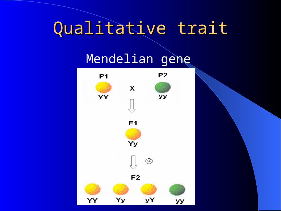
Qualitative traitQualitative trait

Mendelian gene

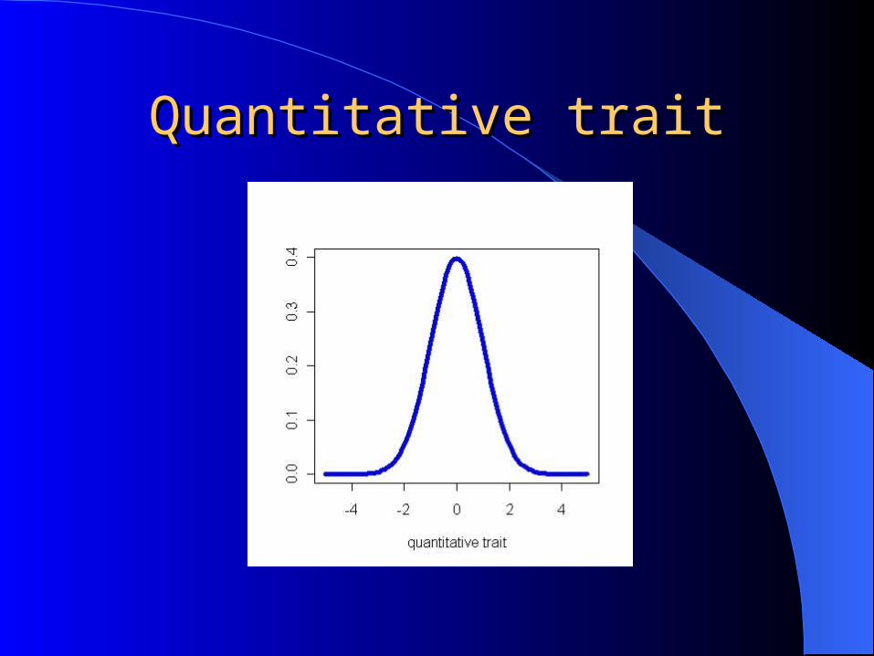
Quantitative traitQuantitative trait

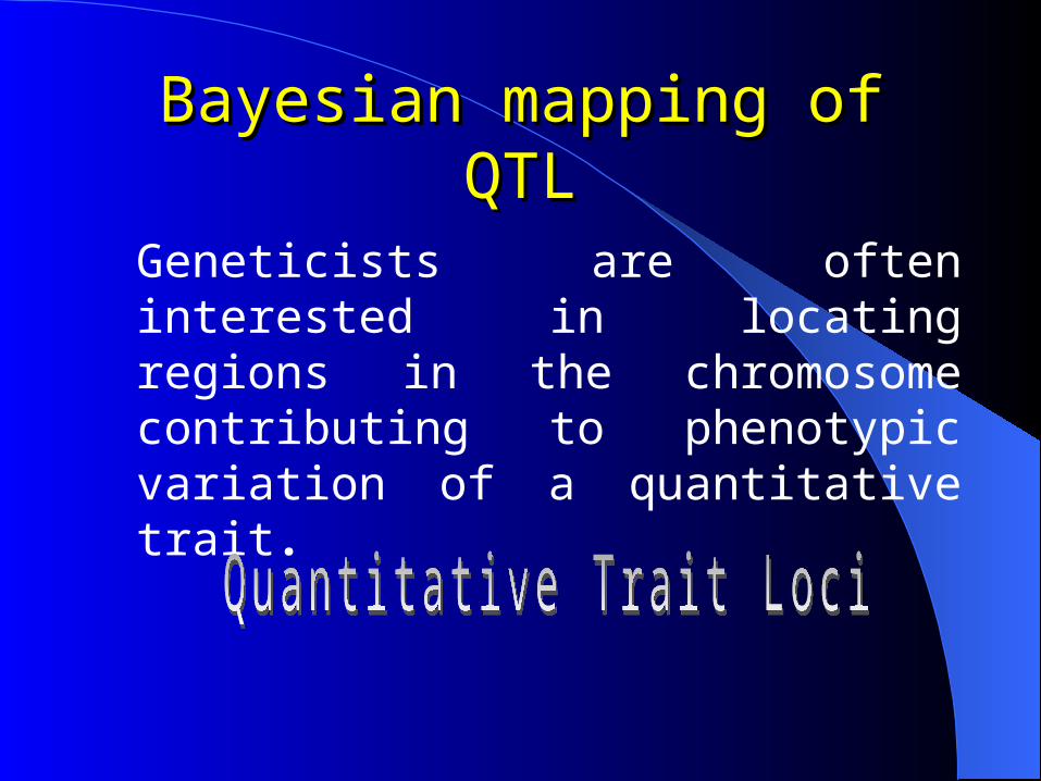
Bayesian mapping of QTLBayesian mapping of QTL

Geneticists are often interested in locating regions in the chromosome contributing to phenotypic variation of a quantitative trait.

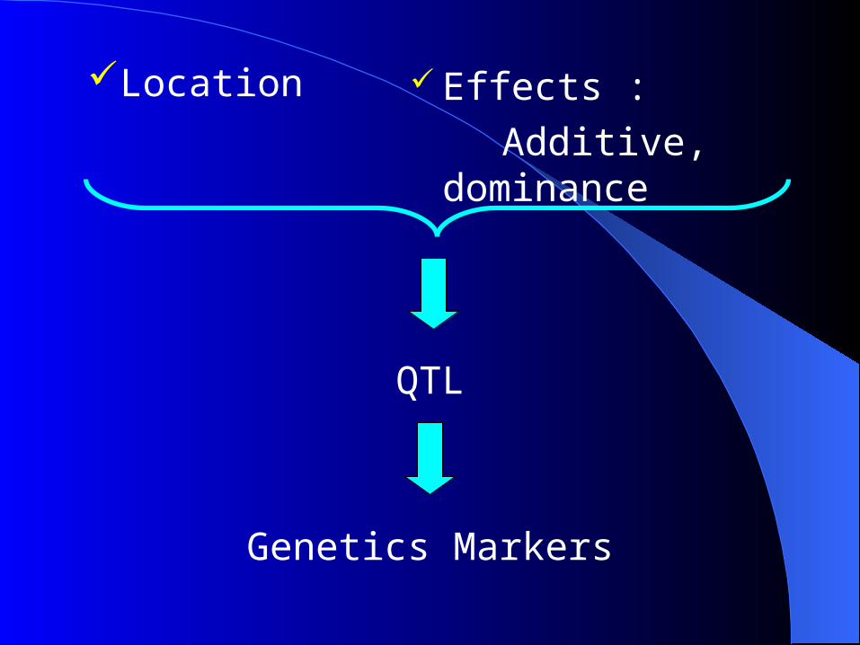
Effects :

Additive, dominance

Location

QTL

Genetics Markers

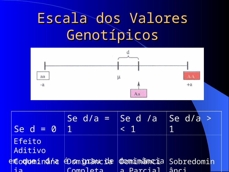
Escala dos Valores Escala dos Valores GenotípicosGenotípicos

Se d = 0 Se d/a = 1 Se d /a < 1 Se d/a > 1Efeito Aditivo

CodominânciaDominância Completa

Dominância Parcial Sobredominânci

em que: d/a é o grau de dominância

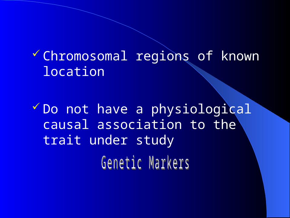
Chromosomal regions of known location

Do not have a physiological causal association to the trait under study

Genetics MarkersGenetics Markers

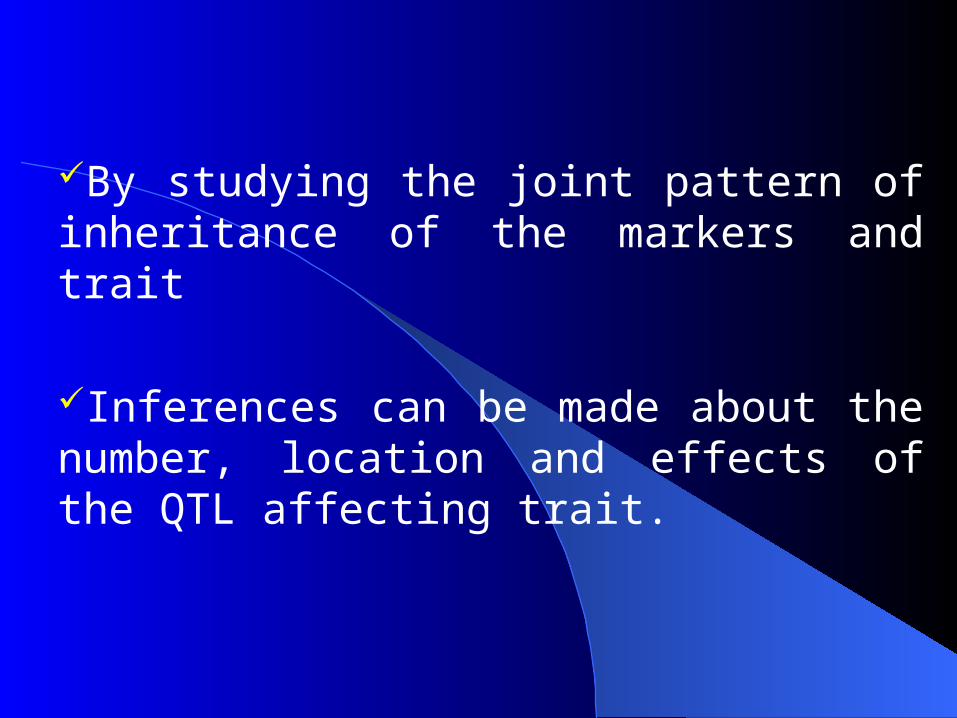
By studying the joint pattern of inheritance of the markers and trait

Inferences can be made about the number, location and effects of the QTL affecting trait.

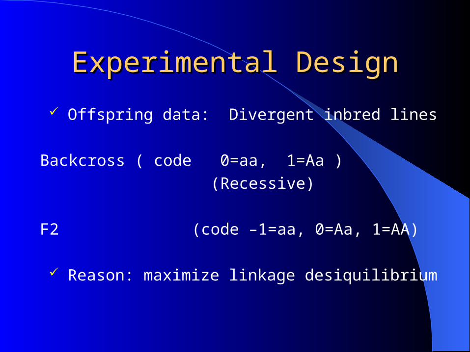
Experimental DesignExperimental Design

Offspring data: Divergent inbred lines

Backcross ( code 0=aa, 1=Aa )

(Recessive)

F2 (code –1=aa, 0=Aa, 1=AA)

Reason: maximize linkage desiquilibrium

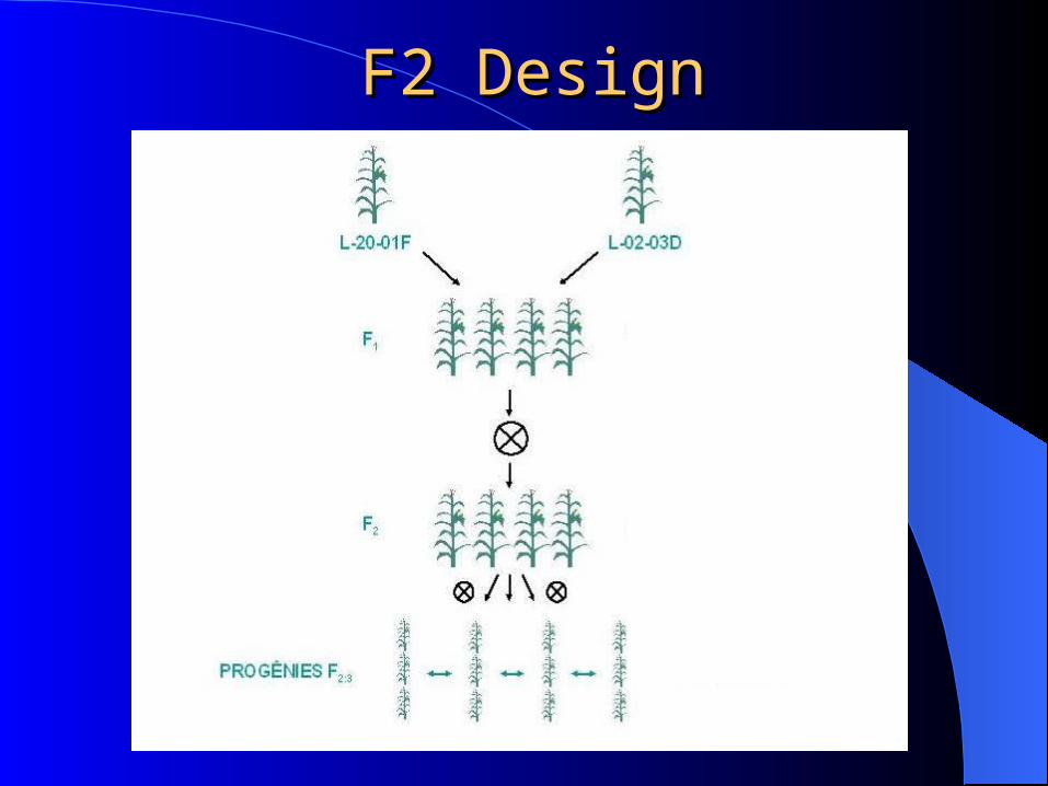
F2 DesignF2 Design

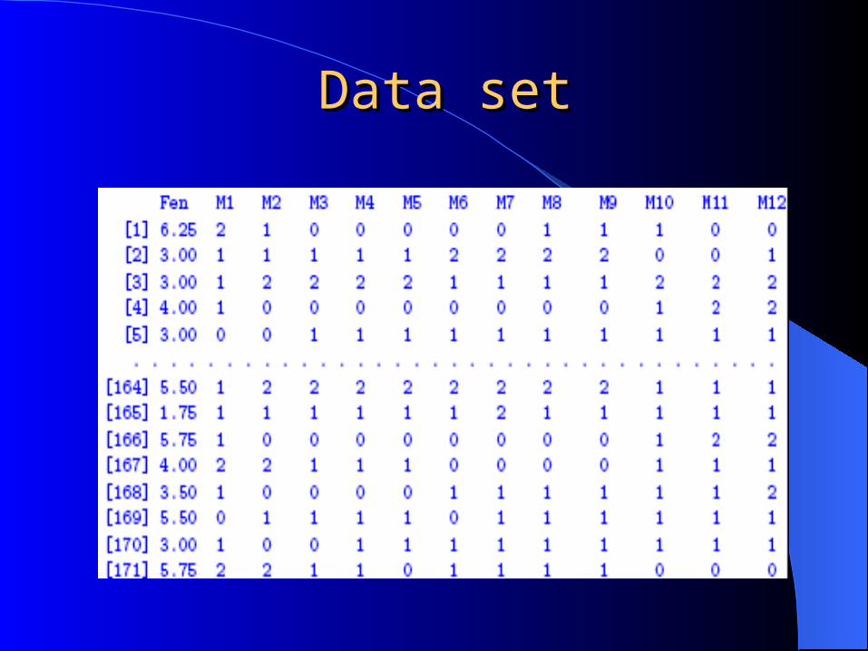
Data setData set

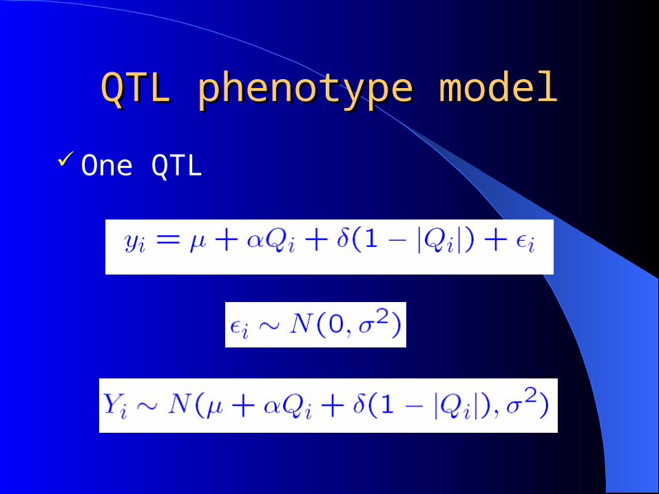
QTL phenotype modelQTL phenotype model

One QTL

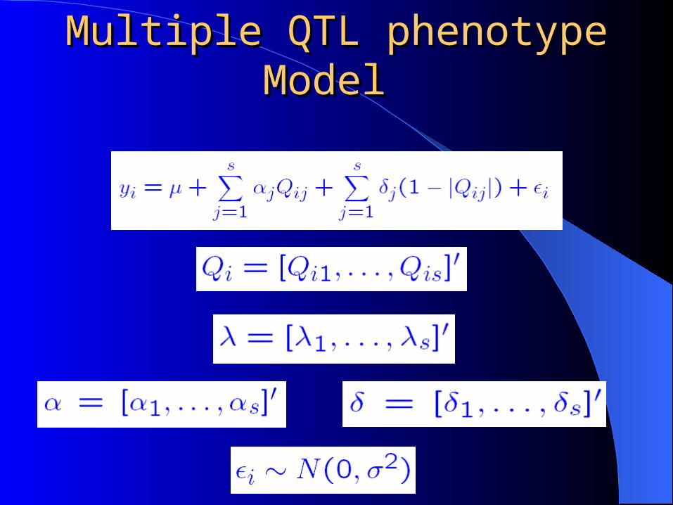
Multiple QTL phenotype Multiple QTL phenotype Model Model

Our aim is to make joint inference about the number of QTL, their positions (loci) and the sizes of their effects.

Assume that a linkage map has been developed for the genome.

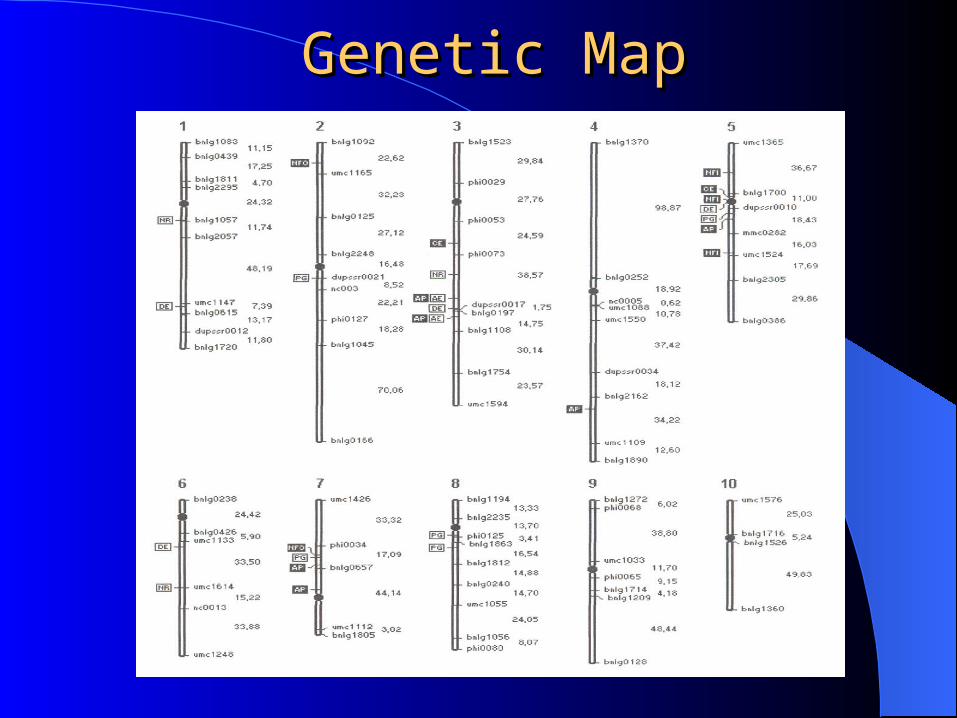
Genetic MapGenetic Map

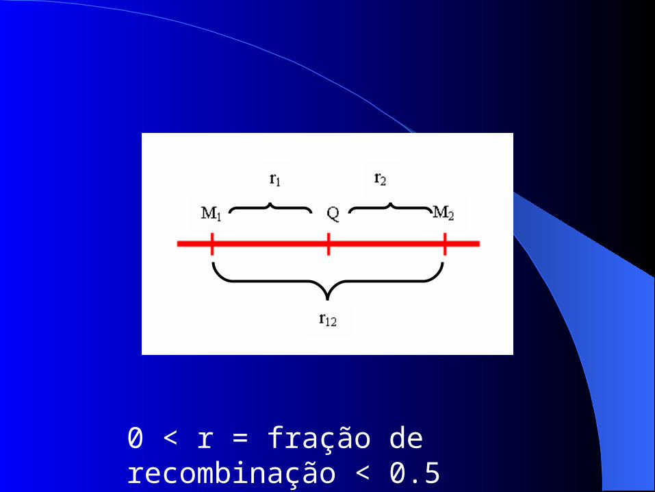
0 < r = fração de recombinação < 0.5

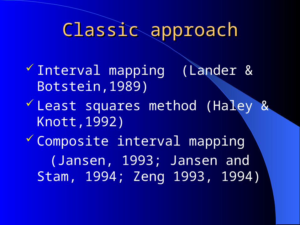
Classic approachClassic approach

Interval mapping (Lander & Botstein,1989)

Least squares method (Haley & Knott,1992)

Composite interval mapping

(Jansen, 1993; Jansen and Stam, 1994; Zeng 1993, 1994)

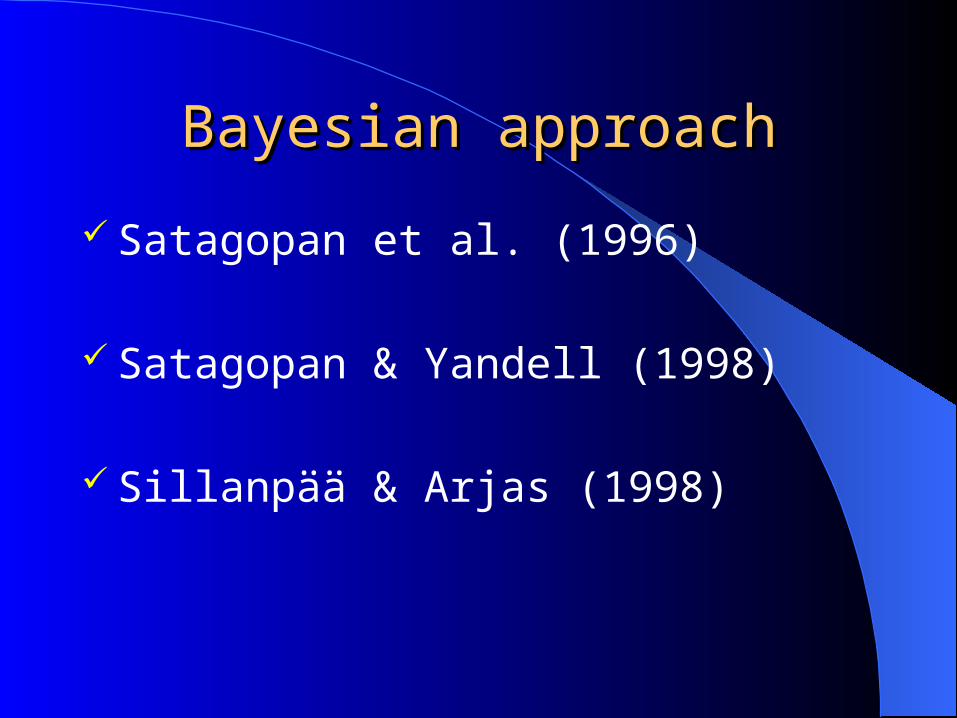
Bayesian approachBayesian approach

Satagopan et al. (1996)

Satagopan & Yandell (1998)

Sillanpää & Arjas (1998)

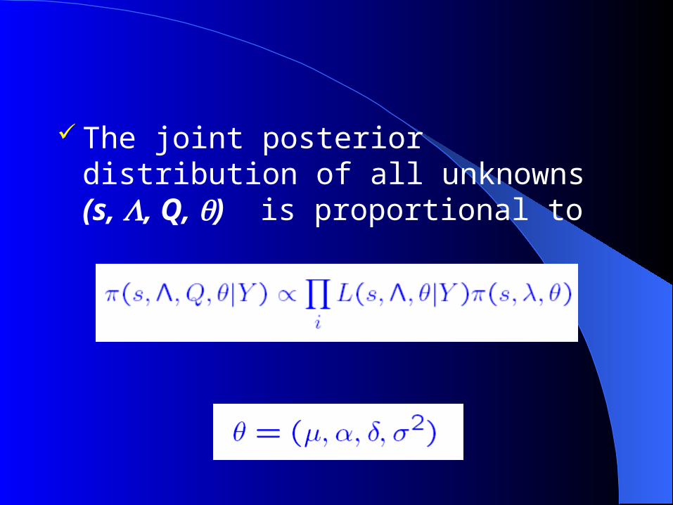
The joint posterior distribution of all unknowns (s, , Q, ) is proportional to

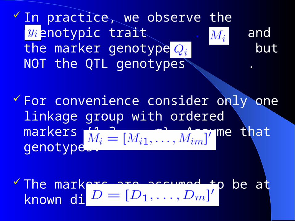
In practice, we observe the phenotypic trait . and the marker genotypes but NOT the QTL genotypes .

For convenience consider only one linkage group with ordered markers {1,2,...,m}. Assume that genotypes:

The markers are assumed to be at known distances

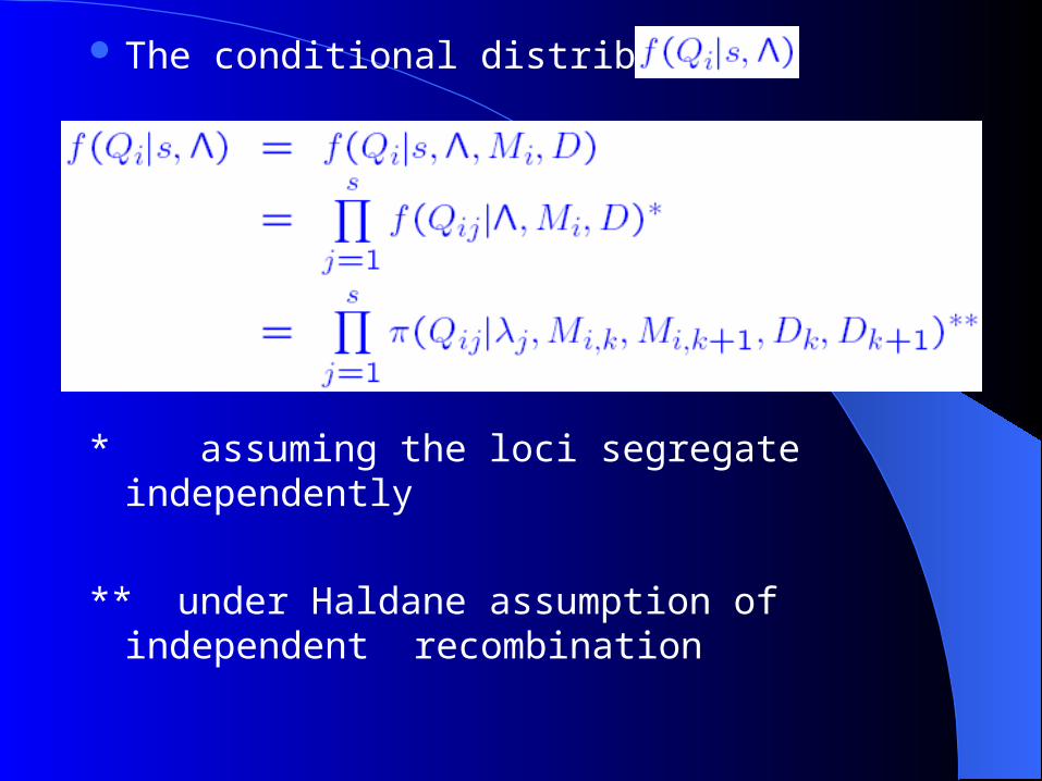
The conditional distribution

* assuming the loci segregate independently

** under Haldane assumption of independent recombination

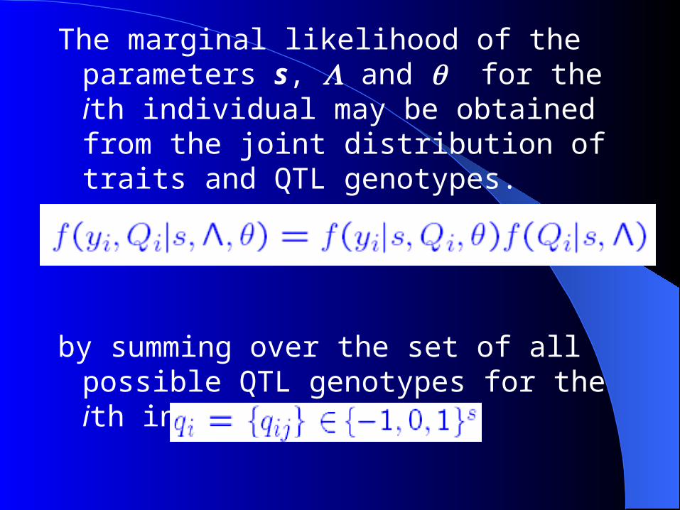
The marginal likelihood of the parameters s, and for the ith individual may be obtained from the joint distribution of traits and QTL genotypes.

by summing over the set of all possible QTL genotypes for the ith individual,

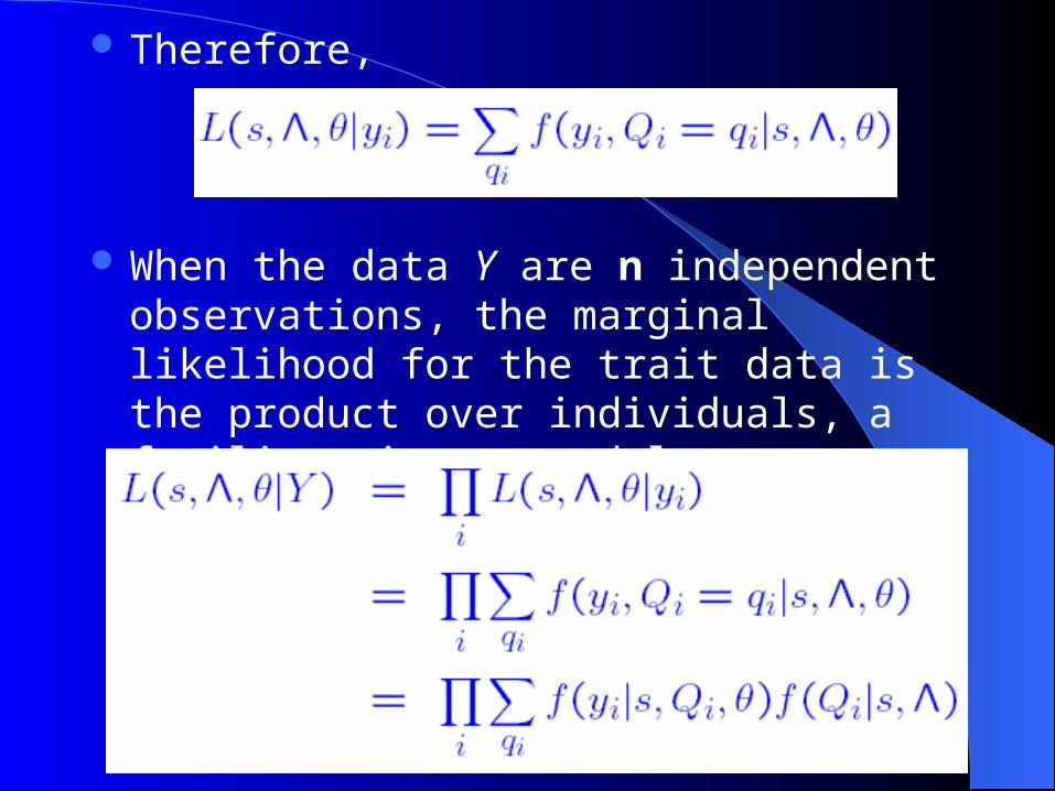
Therefore,

When the data Y are n independent observations, the marginal likelihood for the trait data is the product over individuals, a familiar misture model likelihood,

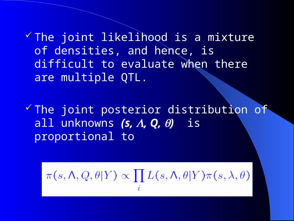
The joint likelihood is a mixture of densities, and hence, is difficult to evaluate when there are multiple QTL.

The joint posterior distribution of all unknowns (s, , Q, ) is proportional to

A Bayesian approach combined with reversible jump MCMC is well suited for QTL studies

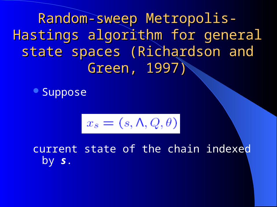
Random-sweep Metropolis-Hastings Random-sweep Metropolis-Hastings algorithm for general state spaces algorithm for general state spaces

(Richardson and Green, 1997)(Richardson and Green, 1997)

Suppose

current state of the chain indexed by s.

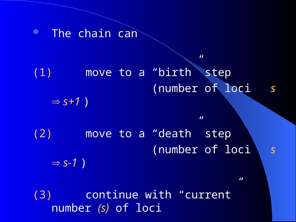
The chain can

(1) move to a “birth” step

(number of loci s s+1 )

(2) move to a “death” step

(number of loci s s-1 )

(3) continue with “current” number (s) of loci

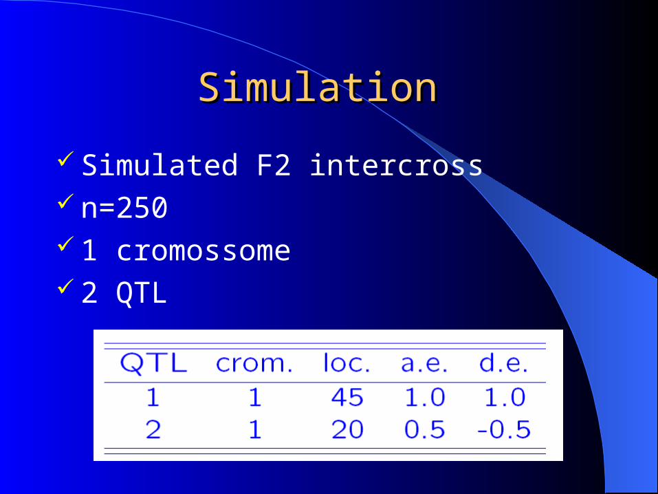
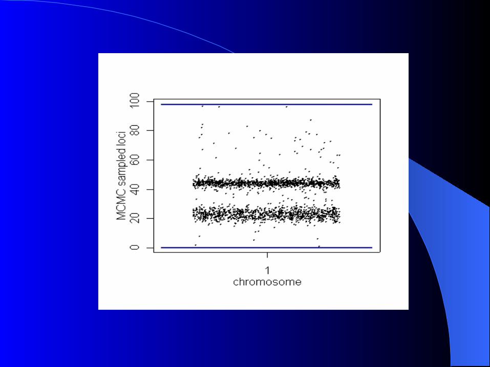
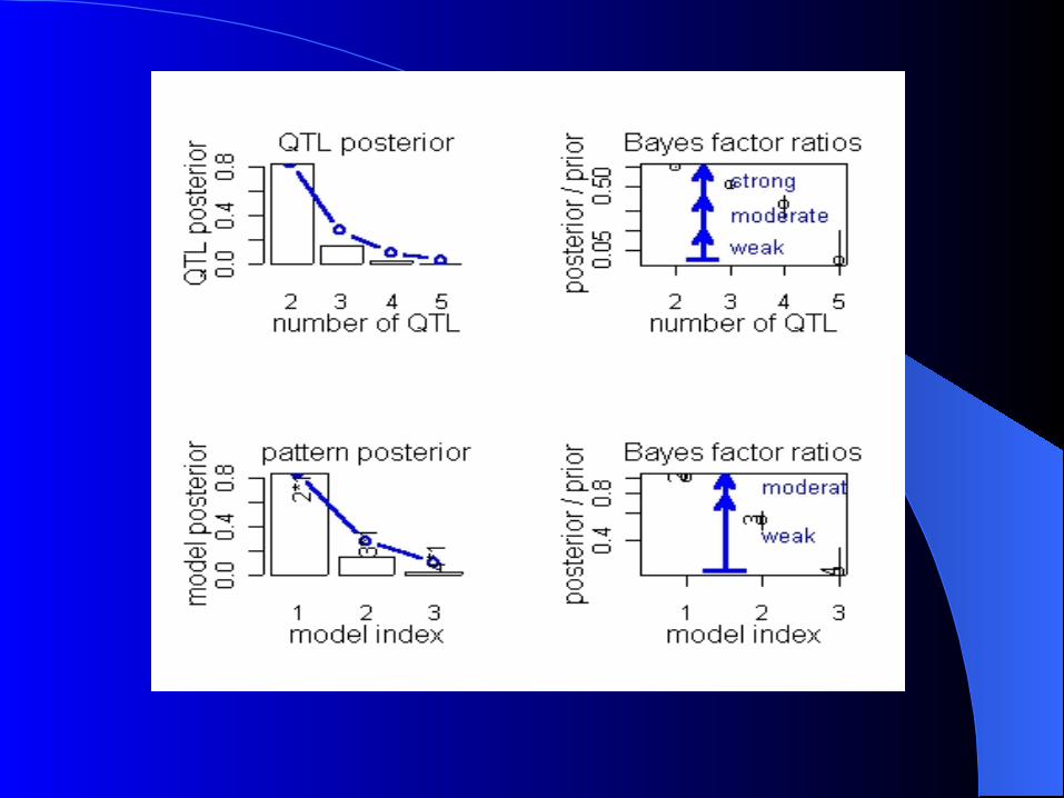
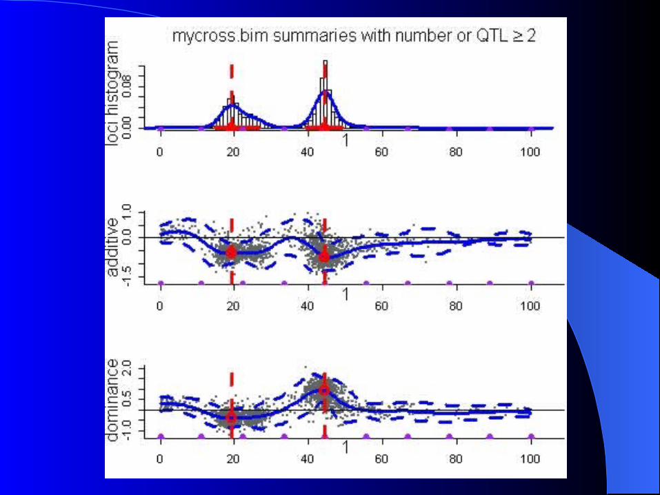
Simulation Simulation

Simulated F2 intercross n=250 1 cromossome 2 QTL

ReferênciasReferências

Satagopan, J. M.; Yandell, B. S. (1998)Bayesian model determination for

quantitative trait