
Numericalinvestigationoftheerosionreduction ... ·...
95
UNIVERSIDADE FEDERAL DE UBERLÂNDIA CARLOS ANTONIO RIBEIRO DUARTE Numerical investigation of the erosion reduction in elbows promoted by a vortex chamber Uberlândia – MG – Brasil 27 de Março de 2015
Transcript of Numericalinvestigationoftheerosionreduction ... ·...

UNIVERSIDADE FEDERAL DE UBERLÂNDIA
CARLOS ANTONIO RIBEIRO DUARTE
Numerical investigation of the erosion reductionin elbows promoted by a vortex chamber
Uberlândia – MG – Brasil
27 de Março de 2015
CARLOS ANTONIO RIBEIRO DUARTE
Numerical investigation of the erosion reduction inelbows promoted by a vortex chamber
Dissertação apresentada ao Programa dePós-Graduação em Engenharia Mecânica daUniversidade Federal de Uberlândia, comoparte dos requisitos para a obtenção dotítulo de MESTRE EM ENGENHARIAMECÂNICA.
Área de concentração: Transferência deCalor e Mecânica dos Fluidos
Universidade Federal de Uberlândia – UFU
Faculdade de Engenharia Mecânica
Programa de Pós-Graduação
Supervisor: Prof. Dr. Francisco José de Souza
Uberlândia – MG – Brasil27 de Março de 2015

Dados Internacionais de Catalogação na Publicação (CIP)Sistema de Bibliotecas da UFU, MG, Brasil.
D812n Duarte, Carlos Antonio Ribeiro, 1989 -2015 Numerical investigation of the erosion reduction in elbows promoted by a vortex
chamber/ Carlos Antonio Ribeiro Duarte. – 2015.95 f. : il.
Orientador: Francisco José de SouzaDissertação (Mestrado) – Universidade Federal de Uberlândia , Programa de
Pós-Graduação em Engenharia Mecânica.Inclui bibliografia
1. Engenharia mecânica - Teses. 2. Desgaste mecânico - Teses. 3. Lagrange,Funções de - Teses. 4. Amortecimento (Mecânica) - Teses. I. Souza, Francisco Joséde. II. Universidade Federal de Uberlândia. III. Programa de Pós-Graduação emEngenharia Mecânica. IV. Título
CDU:621
CARLOS ANTONIO RIBEIRO DUARTE
Numerical investigation of the erosion reduction inelbows promoted by a vortex chamber
Dissertação apresentada ao Programa dePós-Graduação em Engenharia Mecânica daUniversidade Federal de Uberlândia, comoparte dos requisitos para a obtenção dotítulo de MESTRE EM ENGENHARIAMECÂNICA.
Área de concentração: Transferência deCalor e Mecânica dos Fluidos
Trabalho aprovado. Uberlândia – MG – Brasil, 27 de março de 2015:
Prof. Dr. Francisco José de SouzaOrientador - UFU
Prof. Aristeu da Silveira Neto, Dr. Ing.UFU
Waldir Pedro Martignoni, Ph.D.PETROBRAS
Uberlândia – MG – Brasil27 de Março de 2015

To my family for always standing by my side.
Acknowledgements
I would like to express my gratitude to my supervisor, Prof. Dr. Francisco José deSouza, whose expertise, understanding, and patience, added considerably to my graduateexperience. I appreciate his vast knowledge and skill in many areas and his assistance inwriting reports (i.e., publications, conference papers and this dissertation).
A very special thanks goes out to Prof. Dr. Aristeu da Silveira Neto, without whosemotivation and encouragement I would not have considered a graduate career mechanicalengineering research. It was under his tutelage that I developed a focus and becameinterested in computational fluid dynamics. He provided me with direction, technicalsupport and became more of a mentor and friend, than a professor. It was through his,persistence, understanding and kindness that I completed my undergraduate degree andwas encouraged to apply for graduate training. I doubt that I will ever be able to conveymy appreciation fully, but I owe him my eternal gratitude.
Thanks also goes out to those who provided me with technical advice at times ofcritical need; Msc. Bruno Tadeu, Msc. João Rodrigo and Vinicius Fagundes. I would alsolike to thank my friends at MFLab1, for our philosophical debates, exchanges of knowledge,skills, and venting of frustration during my graduate program, which helped enrich theexperience.
I would also like to thank my parents, Maria Beatriz and José Carlos for the supportthey provided me through my entire life, my brother Lucas Eduardo for the friendshipand in particular, I must acknowledge my fiancée and best friend, Larissa, without whoselove, encouragement and patience, I would not have finished this dissertation.
In conclusion, I recognize that this research would not have been possible withoutthe financial assistance of Petróleo Brasileiro (PETROBRAS2), the Coordination forthe Improvement of Higher Education Personnel (CAPES3) , the Federal University ofUberlândia and the Department of Mechanical Engineering, and express my gratitude tothose agencies.
1 MFLAB:<http://mflab.mecanica.ufu.br>2 PETROBRAS <http://www.petrobras.com.br/>3 CAPES <http://www.capes.gov.br/>
"Das Böse existiert nicht,genauso wenig wie die Kälte und die Dunkelheit.
Gott hat das Böse nicht geschaffen.Sondern es ist das Ergebnis dessen,
was Gottes Herz noch nicht berührt hat.”
"Evil does not exist,It is just like darkness and cold,
God did not create evil.Evil is the result of what happens
when man does not have God’s love present in his heart.”
Albert Einstein - (1879 - 1955)

AbstractErosive wear is usually a decisive factor for failure of pipelines plants. Many industrialprocesses which require conveying of erosive particles are directly exposed to problemsof leakage or contamination. As a result, unnecessary costs are needed by maintenanceoperations. This industrial concern is responsible for leading researchers to develop analysistools which can precisely quantify the problem of erosion. Due to this fact, to validate theCFD model, numerical results for the standard elbow are compared to the experimentaldata. After that, a vortex chamber was added to the standard elbow, preserving the samegeometry characteristics (e.g., diameter and curvature radius) as well as the simulationparameters (e.g., initial velocity, density, viscosity, etc.). Based on four-way-coupledsimulations of the gas-solid flow in both geometries, the comparison between the standardand vortex-chamber elbow results was performed and a detailed analysis of the mass loadinginfluence on the flow and on the penetration rate was reached. The present work used thefinite-volume, unstructured code UNSCYFL3D, which solves the gas flow using the fullycoupled Euler-Lagrange approach. The two-layer k-epsilon was used to model turbulenceeffects. Interestingly, the results show that the penetration ratio in the vortex-chamberelbow does not exponentially reduces with the increase of the mass loading, distinguishingfrom the behavior observed in standard elbow. Another important finding is that theaddition of the vortex chamber significantly shows the efficiency of the cushioning effect.Comparing the peak of penetration ratio in both elbow designs for a mass loading of 1.0,the reduction was around 93% when the vortex chamber is present. Therewith, based onnumerical analyses of the coupled gas-solid flow the physical mechanism for the cushioningeffect is proposed.
Key-words: Elbow Erosion, Vortex-chamber Elbow Erosion, Mass Loading, Four-WayCoupling, Inter-Particle Collisions, Cushioning Effect.

ResumoO desgaste erosivo é geralmente um fator decisivo na ruptura de gasodutos. Muitos processosindustriais que necessitam transportar partículas erosivas estão diretamente expostos aproblemas de vazamento ou de contaminação. Como resultado, custos desnecessáriossão usados em operações de manutenção. Essa preocupação industrial é responsável pormotivar os pesquisadores a desenvolver ferramentas de análise que possam quantificar comprecisão o problema da erosão. Devido a esse fato, para validar o modelo de CFD, osresultados numéricos para o cotovelo padrão são comparados com dados experimentais.Depois disso, uma câmara de vórtice foi adicionada ao cotovelo padrão, mantendo asmesmas características geométricas (e.g., diâmetro e raio de curvatura), bem como osparâmetros de simulação (e.g., velocidade inicial, densidade, viscosidade, etc.). Com baseem simulações com quatro vias de acoplamento do escoamento gás-sólido em ambasgeometrias, a comparação entre os resultados de cotovelo padrão e do cotovelo comcâmara de vórtice foi realizada e uma análise detalhada da influência da carga mássica noescoamento e na taxa de penetração foi obtida. O presente trabalho utilizou o código devolumes finitos UNSCYFL3D, que resolve o escoamento de gás usando a abordagem deEuler-Lagrange totalmente acoplada. O modelo k-epsilon duas camadas foi usado paramodelar os efeitos de turbulência. Curiosamente, os resultados mostram que a taxa depenetração no cotovelo com câmara de vórtice não reduz exponencialmente com o aumentoda carga mássica, contradizendo o comportamento observado no cotovelo padrão. Outradescoberta importante é que a adição da câmara de vórtice mostra significativamente aeficiência do efeito de amortecimento. Comparando-se o pico da taxa de penetração emambos os modelos de cotovelo para uma carga mássica de 1.0, a redução foi cerca de 93 %quando a câmara de vórtice está presente. Com base em análises numéricas do escoamentode gás-sólido acoplado, o mecanismo físico do efeito de amortecimento é proposto.
Palavras-chaves: Erosão em Cotovelos, Erosão em Cotovelos com Câmara de Vórtice,Carga Mássica, Quatro-Vias de Acoplamento, Colisões entre Partículas, Efeito de Amortec-imento.

List of Figures
Figure 1 – Example of erosive wear in a pump casing. . . . . . . . . . . . . . . . . 17Figure 2 – Methodology used to reach the research objective. . . . . . . . . . . . . 20Figure 3 – Examples of flow configurations related to erosion due to impact by
solid particles (HUMPHREY, 1990). . . . . . . . . . . . . . . . . . . . 24Figure 4 – Examples of pipe fittings. . . . . . . . . . . . . . . . . . . . . . . . . . 25Figure 5 – Example of a 90 degree elbow. . . . . . . . . . . . . . . . . . . . . . . . 26Figure 6 – Example of a vortex-chamber elbow. . . . . . . . . . . . . . . . . . . . 27Figure 7 – The turbulent kinetic energy distributed over eddies of different sizes
(FRöHLICH; TERZI, 2008). . . . . . . . . . . . . . . . . . . . . . . . . 32Figure 8 – Control volume for a finite volume discretization. . . . . . . . . . . . . 45Figure 9 – Flowchart solution of SIMPLE method implemented in UNSCYFL3D. 47Figure 10 – Flow chart of fully coupled Euler-Lagrange calculations (LAíN; SOM-
MERFELD, 2013). . . . . . . . . . . . . . . . . . . . . . . . . . . . . . 50Figure 11 – Schematics of the elbow investigated. . . . . . . . . . . . . . . . . . . . 52Figure 12 – Standard Elbow domain. . . . . . . . . . . . . . . . . . . . . . . . . . . 53Figure 13 – Schematics of the vortex-chamber elbow investigated. . . . . . . . . . . 54Figure 14 – Vortex-Chamber Elbow domain. . . . . . . . . . . . . . . . . . . . . . . 55Figure 15 – Streamlines of the velocity field inside the standard elbow. . . . . . . . 56Figure 16 – Erosion contours of mass loading φ = 0.013 with different levels of
interaction: (a) One-way coupling; (b) Two-way coupling; (c) Four-waycoupling. . . . . . . . . . . . . . . . . . . . . . . . . . . . . . . . . . . . 57
Figure 17 – Numerical and experimental penetration ratios versus bend curvatureangle for one, two and four-way couplings. Mass loading φ = 0.013. . . 58
Figure 18 – Erosion contours of mass loading φ = 0.25 with different phase interac-tion regimes: (a) One-way coupling; (b) Two-way coupling; (c) Four-waycoupling. . . . . . . . . . . . . . . . . . . . . . . . . . . . . . . . . . . . 58
Figure 19 – Numerical and experimental penetration ratio versus bend curvatureangle for one, two and four-way coupling and mass loading φ = 0.25. . 59
Figure 20 – Influence of two-way (lines with symbols) and four-way (dashed lines)coupling for φ = 0.25 and φ = 1.0. . . . . . . . . . . . . . . . . . . . . . 60
Figure 21 – Average velocity field for the fluid (continuous line), particles in two-waycoupling (circles) and particles in four-way coupling (squares). Massloading is φ = 1.0. . . . . . . . . . . . . . . . . . . . . . . . . . . . . . 61
Figure 22 – Influence of the mass loading in the penetration ratio. . . . . . . . . . . 62

Figure 23 – Snapshot of particle behavior for φ = 1.0. From top to bottom: one-way,two-way and four-way couplings. From left to right: before collision withthe bend outer surface, during collision with bend, and during collisionwith the wall, as seen from the side opposing the inlet domain. . . . . . 63
Figure 24 – Erosion contours with four-way coupling approach for the growing massloadings: (a) φ = 0.013; (b) φ = 0.25; (c) φ = 0.5; (d) φ = 1.0; (e) φ = 1.5. 64
Figure 25 – Particle concentration field for mass loading φ = 1.0: (a) One-waycalculation; (b) Two-way calculation; (c) Four-way calculation. . . . . . 65
Figure 26 – Streamlines of the velocity field inside the vortex-chamber elbow. . . . 66Figure 27 – Contours of velocity magnitude (a) and turbulence kinetic energy (b)
in symmetry plane. . . . . . . . . . . . . . . . . . . . . . . . . . . . . . 67Figure 28 – Erosion contours of mass loading φ = 0.013 with different phase interac-
tion regimes: (a) One-way coupling; (b) Two-way coupling; (c) Four-waycoupling. . . . . . . . . . . . . . . . . . . . . . . . . . . . . . . . . . . . 68
Figure 29 – Numerical penetration ratio versus bend curvature angle for one, twoand four-way couplings. Mass loading φ = 0.013. . . . . . . . . . . . . . 68
Figure 30 – Erosion contours of mass loading φ = 0.25 with different phase interac-tion regimes: (a) One-way coupling; (b) Two-way coupling; (c) Four-waycoupling. . . . . . . . . . . . . . . . . . . . . . . . . . . . . . . . . . . . 69
Figure 31 – Numerical penetration ratio versus bend curvature angle for one, twoand four-way couplings. Mass loading φ = 0.25. . . . . . . . . . . . . . 70
Figure 32 – Erosion contours with two-way coupling approach for the growing massloadings: (a) φ = 0.013; (b) φ = 0.25; (c) φ = 0.5; (d) φ = 1.0; (e) φ = 1.5. 71
Figure 33 – Numerical penetration ratio versus bend curvature angle with two-waycoupling approach for the growing mass loadings: (a) φ = 0.013; (b)φ = 0.25; (c) φ = 0.5; (d) φ = 1.0; (e) φ = 1.5. . . . . . . . . . . . . . . 71
Figure 34 – Average velocity inside the vortex chamber: (a) fluid, (b) particle. . . . 72Figure 35 – Erosion contours with four-way coupling approach for the growing mass
loadings: (a) φ = 0.013; (b) φ = 0.25; (c) φ = 0.5; (d) φ = 1.0; (e) φ = 1.5. 73Figure 36 – Erosion contours with four-way coupling approach for the growing mass
loadings: (a) φ = 0.013; (b) φ = 0.25; (c) φ = 0.5; (d) φ = 1.0; (e)φ = 1.5 and fixed for φ = 1.5 magnitude. . . . . . . . . . . . . . . . . . 74
Figure 37 – Numerical penetration ratio versus bend curvature angle with four-waycoupling approach for the growing mass loadings: (a) φ = 0.013; (b)φ = 0.25; (c) φ = 0.5; (d) φ = 1.0; (e) φ = 1.5. . . . . . . . . . . . . . . 75
Figure 38 – Particle concentration field for mass loading φ = 1.5: (a) One-waycalculation; (b) Two-way calculation; (c) Four-way calculation. . . . . . 75
Figure 39 – Comparison between the standard and the vortex-chamber elbows. . . 77
Figure 40 – Standard elbow fields: (a) U velocity component; (b) V velocity compo-nent; (c) W velocity component. . . . . . . . . . . . . . . . . . . . . . . 88
Figure 41 – Standard elbow fields: (a) Pressure; (b) Turbulence Kinetic Energy. . . 88Figure 42 – Vortex-chamber elbow fields: (a) U velocity component; (b) V velocity
component; (c) W velocity component. . . . . . . . . . . . . . . . . . . 89Figure 43 – Vortex-chamber elbow fields: (a) Pressure; (b) Turbulence Kinetic Energy. 89Figure 44 – Snapshot of particle behavior inside the standard elbow colored by
diameter (one-way coupling). . . . . . . . . . . . . . . . . . . . . . . . 90Figure 45 – Snapshot of particle behavior inside the standard elbow colored by
rotation: blue - low, red - high (one-way coupling). . . . . . . . . . . . 91Figure 46 – Snapshot of particle behavior inside the vortex-chamber elbow colored
by diameter (one-way coupling). . . . . . . . . . . . . . . . . . . . . . . 92Figure 47 – Snapshot of particle behavior inside the vortex-chamber elbow colored
by rotation: blue - low, red - high (one-way coupling). . . . . . . . . . . 93Figure 48 – Snapshot of particles behavior for φ = 1.0. From top to bottom: 0.39s,
0.5s and 0.8s. From left to right: one-way, two-way and four-way coupling. 94

List of Tables
Table 1 – Constants used for the erosion ratio correlation. . . . . . . . . . . . . . . 42Table 2 – Simulation conditions for erosion prediction. . . . . . . . . . . . . . . . 53Table 3 – Standard elbow (SE) and vortex-chamber elbow (VCE) peak reduction. 77

List of abbreviations and acronyms
CFD Computational Fluid Dynamics
DES Detached Eddy Simulation
DNS Direct Numerical Simulation
FVM Finite Volume Method
LES Large Eddy Simulation
MFlab Laboratory of Fluid Mechanics
NSE Navier Stokes Equation
NPS Nominal Pipe Size
PETROBRAS Petróleo Brasileiro
RANS Reynolds-Averaged Navier–Stokes equations
RMS Root Mean Square
SIMPLE Semi-Implicit Method for Pressure-Linked Equations
TKE Turbulence Kinetic Energy

List of symbols
δij Kronecker delta
gi Gravity component

Contents
1 INTRODUCTION . . . . . . . . . . . . . . . . . . . . . . . . . . . . 17
2 DISSERTATION SCOPE . . . . . . . . . . . . . . . . . . . . . . . . 192.1 Research objective . . . . . . . . . . . . . . . . . . . . . . . . . . . . . 192.2 Relevance . . . . . . . . . . . . . . . . . . . . . . . . . . . . . . . . . . 202.3 Methodology . . . . . . . . . . . . . . . . . . . . . . . . . . . . . . . . 20
3 BACKGROUND THEORY . . . . . . . . . . . . . . . . . . . . . . . 223.1 Types of wear . . . . . . . . . . . . . . . . . . . . . . . . . . . . . . . . 223.1.1 Erosion due to particles . . . . . . . . . . . . . . . . . . . . . . . . . . . . 223.1.2 Erosion mechanisms . . . . . . . . . . . . . . . . . . . . . . . . . . . . . 233.1.3 Influence of the flow in the erosion . . . . . . . . . . . . . . . . . . . . . . 243.2 Pipe fittings . . . . . . . . . . . . . . . . . . . . . . . . . . . . . . . . . 253.2.1 Standard elbow . . . . . . . . . . . . . . . . . . . . . . . . . . . . . . . . 253.2.2 Vortex-chamber elbow . . . . . . . . . . . . . . . . . . . . . . . . . . . . 263.3 CFD applied to erosion problems . . . . . . . . . . . . . . . . . . . . . 273.3.1 Erosion correlations . . . . . . . . . . . . . . . . . . . . . . . . . . . . . . 273.3.2 Coefficients of restitution . . . . . . . . . . . . . . . . . . . . . . . . . . . 293.3.3 Coefficients of friction . . . . . . . . . . . . . . . . . . . . . . . . . . . . 30
4 MATHEMATICAL MODELS . . . . . . . . . . . . . . . . . . . . . . 314.1 Gas phase equations . . . . . . . . . . . . . . . . . . . . . . . . . . . . 314.1.1 Reynolds Averaged Navier Stokes simulations . . . . . . . . . . . . . . . . 334.1.2 Turbulence model . . . . . . . . . . . . . . . . . . . . . . . . . . . . . . . 344.1.2.1 Two layer k − ε model . . . . . . . . . . . . . . . . . . . . . . . . . . . . . . 34
4.2 Particle motion equations . . . . . . . . . . . . . . . . . . . . . . . . . 364.3 Erosion prediction equation . . . . . . . . . . . . . . . . . . . . . . . . 40
5 FINITE VOLUME DISCRETIZATION . . . . . . . . . . . . . . . . . 435.1 Finite Volume Method . . . . . . . . . . . . . . . . . . . . . . . . . . . 435.2 Spatial discretization . . . . . . . . . . . . . . . . . . . . . . . . . . . . 435.3 Pressure-velocity coupling . . . . . . . . . . . . . . . . . . . . . . . . . 455.4 Solution procedure . . . . . . . . . . . . . . . . . . . . . . . . . . . . . 465.5 Solver UNSCYFL3D . . . . . . . . . . . . . . . . . . . . . . . . . . . . 47
6 PARTICLE PHASE ALGORITHM . . . . . . . . . . . . . . . . . . . 496.1 Coupling procedure . . . . . . . . . . . . . . . . . . . . . . . . . . . . . 49

6.2 Particle-tracking algorithm . . . . . . . . . . . . . . . . . . . . . . . . 51
7 NUMERICAL SETUP AND PROCEDURE . . . . . . . . . . . . . . 52
8 RESULTS . . . . . . . . . . . . . . . . . . . . . . . . . . . . . . . . . 568.1 Standard elbow results . . . . . . . . . . . . . . . . . . . . . . . . . . . 568.1.1 Validation at low concentration - One, two and four-way couplings . . . . . 568.1.2 Two-way versus four-way coupling . . . . . . . . . . . . . . . . . . . . . . 608.1.3 Influence of the mass loading in the penetration ratio . . . . . . . . . . . . 618.1.4 Mechanisms of particle interactions - Cushioning effect . . . . . . . . . . . 658.2 Vortex-chamber elbow results . . . . . . . . . . . . . . . . . . . . . . 668.2.1 Fluid phase simulation . . . . . . . . . . . . . . . . . . . . . . . . . . . . 668.2.2 Effects at low concentration - One, two and four-way coupling . . . . . . . 678.2.3 Two-way coupling . . . . . . . . . . . . . . . . . . . . . . . . . . . . . . . 708.2.4 Influence of the mass loading in the penetration ratio - Four-way coupling . 728.2.5 Mechanisms of erosion reduction . . . . . . . . . . . . . . . . . . . . . . . 758.2.6 Standard elbow versus Vortex-chamber elbow . . . . . . . . . . . . . . . . 76
9 CONCLUSIONS . . . . . . . . . . . . . . . . . . . . . . . . . . . . . 78
10 FUTURE RESEARCH . . . . . . . . . . . . . . . . . . . . . . . . . . 80
Bibliography . . . . . . . . . . . . . . . . . . . . . . . . . . . . . . . 81
APPENDIX 86
APPENDIX A – ADDITIONAL ILLUSTRATIONS . . . . . . . . . 87
17
1 Introduction
Particles carried by a fluid flow is a common situation in many engineering systems.The necessity to model and predict detailed information about these kind of flows became apersistent issue in the study of multiphase flows over the past few decades. By understandingthe dynamics of motion, it is possible to make improvements and increase the safety duringthe operation of these systems.
Throughout the 60’s a new theoretical approach has been developed, the Computa-tional Fluid Dynamics (CFD). The Computational Fluid Dynamics aims to simulate flowthrough numerical methodologies designed to represent a physical phenomenon. Althoughits development begun over 50 years ago, only in the 90’s it started to have greater accep-tance in the industry, especially in aeronautical projects. Nowadays, the ComputationalFluid Dynamics has become an important tool to study flow problems, helping designersto optimize single and multiphase systems. In wear-related problems, the CFD is used as atool for predicting the wear in various environments and due to its complexity unfeasiblethe use of empirical correlations.
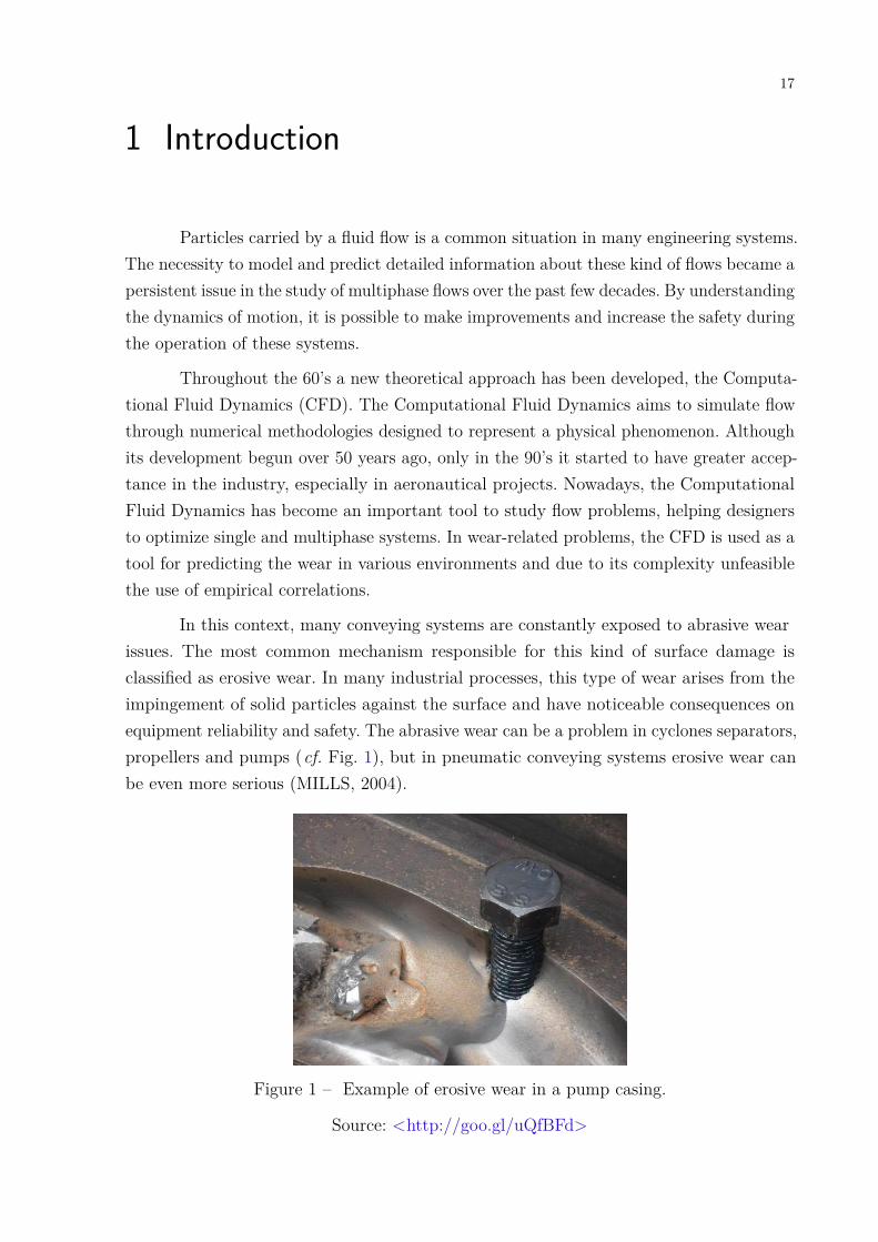
In this context, many conveying systems are constantly exposed to abrasive wearissues. The most common mechanism responsible for this kind of surface damage isclassified as erosive wear. In many industrial processes, this type of wear arises from theimpingement of solid particles against the surface and have noticeable consequences onequipment reliability and safety. The abrasive wear can be a problem in cyclones separators,propellers and pumps (cf. Fig. 1), but in pneumatic conveying systems erosive wear canbe even more serious (MILLS, 2004).
Figure 1 – Example of erosive wear in a pump casing.
Source: <http://goo.gl/uQfBFd>

Chapter 1. Introduction 18
Generally speaking, erosive wear is a problem which industry has learned to live.Although there are many ways to reduce the magnitude of the problem, relate the conveyedmaterial and the system itself requires a large number of variables to be taken into account.In addition, maintenance time and operating costs are also important factors that leadcompanies to decide which is the best method for the reduction of erosion in their equipment.For an entire pipeline plant, the effects of different elements (e.g., constrictions, pipe shapesand pipe fittings) have to be considered. Due to the nature of the transport process, pipingsystems are willing to wear when abrasive particles have to be conveyed. When particlesare carried in suspension through the air, high conveying air velocities are required to keepthe material moving, in order to prevent pipeline obstruction. In this context, pipe fittingsprovide pneumatic conveying systems with their flexibility in change the flow direction,however, these spots become more susceptible to repeatedly collisions and rapid wear canoccur.
The goal of this dissertation is to support oil and gas industry by analyzing themechanisms responsible for the erosion reduction in elbows promoted by a vortex chamber.In agreement with both Petróleo Brasileiro (PETROBRAS) as well as the supervisor fromthe university, and supported by the acquired knowledge during the literature review, itwas decided to focus the research on the erosion reduction with the increase of the massloading for both standard and vortex-chamber elbows.
The present dissertation is organized as follows: Chapter 2 discusses the objectiveand the method to reach it. In chapter 3, the background theory is presented as wellas an overview of the elbows studied. Chapter 4 presents an overview of the relevantequations for gas/particle phase and erosion prediction. Chapters 5 and 6 describes thetype of discretization and the particle phase algorithm, respectively. Chapter 7 presentsa summary of the experiments and the numerical approach applied.The dissertation isconcluded in Chapter 9 and future research recommendation are given in Chapter 10.

19
2 Dissertation scope
After an exhaustive literature review, for a successful and fulfillment of the gradu-ation research, it is of extreme importance to define the goal and a method to reach it.Both are elaborate in this chapter. First Section 2.1 presents the research objective, afterwhich a few words are spend on the relevance of the project in Section 2.2. Finally, inSection 2.3, a methodology is presented in order to reach the objective.
2.1 Research objectiveThere are two factors that directly influenced the definitive research objective of
the current dissertation. Besides the literature acquired during the literature research, thesuggestions and advices from the university supervisor are taken into account. PETRO-BRAS project suggestions are focused on solve problems related to wear in oil and gasindustry, whereas my supervisor also draw attention to the scientific value of the research.For this reason, the research objective is divided into a primary and secondary objective.
The first objective relates to the research from a scientific perspective. This objectiveforms the basis to complete the research.
Carry out an investigation of the mass loading effects on the erosion of aninety-degree-elbow, by simulating the elbow with an in-house CFD code.
The reason for focusing on the ninety-degree-elbow is related to validate the erosionprediction model with experiments, implement it in the code and analyze its capacity todeal with a variety of erosion problems in engineering with sufficient accuracy.
The second objective covers the part of the research that is of particular interestfor PETROBRAS.
Predict the erosion profile in a vortex-chamber elbow for different mass loadings,aiming to verify its benefits when compared with the standard elbow geometry.
The reduction of erosion in cyclones separators and conveying systems are ofparticular interest for the company. For engineering purpose they require to know themagnitude of erosion acting on the equipment surface and the effects of the mass loadingon the erosive process.
Both objectives are fulfilled simultaneously throughout this dissertation, whereasthe conclusions can be found in Chapter 9.

Chapter 2. Dissertation scope 20
2.2 RelevanceFor this research, the only available simulation tool is CFD. Unfortunately erosion
experimenting and measuring are not feasible. During the literature survey no example ofsolely the application of CFD onto a vortex-chamber elbow was found. Hence it would berather novel to produce useful results using solely CFD. The standard elbow validationprocess will form one of the key parts in successfully acquiring these results. So besides thebenefits for PETROBRAS, the research will also contribute to the scientific community.
2.3 MethodologyKnowing the research objectives it is possible to outline an initial methodology.
This process is devised with the knowledge obtained during the literature review. It isschematically showed in Fig. 2 by placing the various steps in blocks and connecting themvia arrows.
ValidationFphaseF-FStandardFElbow
AnalysisFphaseF-FStandardFElbow
AnalysisFphaseF-FVortex-chamberFElbow
InitialFsetup SolveFsimulationCompareFtoF
experimentalFdata
UpdateFsetup
AlterFsetupSolveFsimulationCompareFtoF
experimentalFdata
UpdateFsetup
Alt
erFg
eom
etry
AlterFsetup SolveFsimulation AnalyseFflowF
behavior
UpdateFsetup
FinalF
recommendations
Figure 2 – Methodology used to reach the research objective.

Chapter 2. Dissertation scope 21
Two phases can be distinguished; a validation phase and an analysis phase. Thegoal of the validation phase is to come up with a simulation setup that provides sufficientlyaccurate results in order to be used for the standard elbow simulations. In the analysisphase, both standard and vortex-chamber elbows are simulated for different values of massloadings. The next lines explain both phases in details.
Validation phaseFor the standard elbow an initial simulation setup is created based on literature and
different erosion prediction models are tested. After find the best model, the simulation isran and the resulting erosion profile is compared to existing experimental data. Dependingon the outcome, the setup is updated in order to match both data sets more closely.Note that the updates are based on acquired literature and preserves the experimentalcharacteristics. The complete validation phase is covered in Section 8.1.1 of this report.
Analysis phaseOnce the simulation shows good agreement with the experimental data, the setup
is altered such that it solves the flow and the erosion for different mass loadings. Theresulting simulations can provide important insight into the changes of the erosion profiledue to the mass loading variations. After this stage, the vortex-chamber geometry iscreated and the validate standard elbow simulation setup serves as an initial setup for thevortex-chamber simulations.
Finally, the vortex-chamber elbow is simulated with various mass loadings whileusing the best known simulation setup employed for the standard elbow. By analyzingthe resulting dataset, it becomes possible to obtain remarkable results on both elbowssimulations. The complete analysis phase is covered in Sections 8.1 and 8.2 of this report.
However before elaborating the research objective, first some background theory isrequired. This should provide the reader with a basic understanding of erosion wear andnumerical techniques to compute them. The following set of chapters, bundled in Chapters3 to 6, presents this theory.

22
3 Background theory
Several characteristics make the erosion profile inside pipelines and elbows signifi-cantly different. Hence the Computational Fluid Dynamical (CFD) techniques required tosimulated the flow differ as well. This part of the dissertation will present the backgroundtheory required to understand the basic erosion phenomena occurring inside pipes and theCFD techniques employed to simulate them.
3.1 Types of wearAs described in many books, (e.g., Gahr (1987) and Hutchings (1992)), different
types of wear may be separated by referring to the basic material removal mechanisms, thewear mechanisms, that cause the wear on a microscopic level. There are many attemptsto classify wear by wear mechanisms, but a commonly accepted first order classificationdistinguishes between adhesive wear, abrasive wear, wear caused by surface fatigue, andwear due to tribochemical reactions.
Very commonly, the damage observed on a tribologically loaded surface is a result oftwo or more coexisting or interacting surface damage types. Interacting damage types maylead to unproportionally high wear rates, as for example in oxidation-enhanced surfacecracking; adhesive wear may however also be suppressed by oxidation (ASKELAND;FULAY; WRIGHT, 2010).
In this context, the present dissertation will exclusively focus on the erosion dueto particles. It is known that other types of wear can coexist, however, carry out a studywith more than one type of wear at the same time can significantly increase the difficultyto find accurate mathematical models. Due to this fact, all the geometries studied in thisreport as well as the experimental database have their surface damaged preferentiallyby erosion, avoiding the interference of other types of wear and facilitating an accurateanalysis of the models used in the simulations.
3.1.1 Erosion due to particles
Erosion is defined as the wear resulted by the interaction between a solid surfaceand a fluid flow containing abrasive particles with a certain speed, or the impact of freemoving liquid (or solid) particles on a solid surface (FINNIE, 1960). We can divide theunderstanding of erosion in two major parts, the first being the determination of thefluid flow conditions of the number, direction, and velocity of the particles striking thesurface. The second part may be defined as the calculation of surface material removed,

Chapter 3. Background theory 23
with the data acquired from the first part. Clearly, the first part of the erosion process ischaracterized as a fluid mechanics problem, with the fluid flow transporting the particlesinto the surface, which defines the erosion wear (PEREIRA; SOUZA; MORO, 2014).
Erosion wear is dependent of the number of particles striking a surface, as well as thephysical quantities associated with it, such as particle velocity and their direction relativeto the surface to be struck. It is known that these quantities are noticeably determinedby the flow conditions. In other words, any minor change in the flow conditions such asviscous regime or temperature might bring large variations in the erosion rate. For example,in operations where the flow direction changes quickly such as turbine blade erosion isusually more severe than in a straight run of piping. Other erosion-increasing factor is thelocal turbulence generated from roughened surface or misaligned parts (FINNIE, 1960).
3.1.2 Erosion mechanisms
According to the literature, there are several ways to describe the mechanism oferosion, as provided from different authors. Therefore, it is difficult to establish only onemechanism as the most reliable and real mechanism. The most used in the literature arethe ones proposed by Finnie (1960) and Hutchings (1992).
Finnie (1960) proposed a mechanism of erosion in which the particle acts as aminiature machine tool in which the surface material is cut, generating a chip. Also, forthe erosion of ductile metals, at oblique impact, this mechanism happens irrespective ofits shape and size.
Hutchings (1992) proposed a similar mechanism. However, he split the cuttingaction into three different types, relying on the shape and the orientation of the erodingparticle. The first type occurs when there is erosion by oblique impact of spherical particles,and the material is removed by a plowing action, moving materials to the front and sideof the particle. The second and third types occur when there is the collision of angularshaped particles, and they differ from each other in the orientation of the erodent particleas it strikes the target surface, as well as the direction of the particle during the contactwith the surface; in other words, if the particle rolls forward or backward during contact.Type I cutting is defined when the particle rolls forward during the contact, and material isremoved by repeated impacts on a prominent lip formed by the indenting angular particle.Type II cutting is defined when the particle rolls backward, and the material is removedas if the erosion was a machining operation, with the material being removed as a chipdue to the fact that there’s a sharp tip of the erodent particle, working as a machiningtool (HUTCHINGS, 1992).

Chapter 3. Background theory 24
3.1.3 Influence of the flow in the erosion
Figure 3 shows four flow configurations commonly found in engineering applications.The first configuration illustrates an impinging jet, which covers a wide range of applications,representing from research configurations to abrasion machining; Figure 3b shows the flowconfiguration found in flows over turbine blades and turbo machinery; Figure 3c showsthe flow configuration that occurs in pneumatic transport of solids and in piping; Figure3d represents the flow configuration found in heat transfer devices (HUMPHREY, 1990).
Figure 3 – Examples of flow configurations related to erosion due to impact by solidparticles (HUMPHREY, 1990).
The dynamic behavior of large and small particles is interpreted briefly in Fig. 1.The ability of a particle to respond to changes imposed by the flow, and therefore, changeits trajectory is characterized by the number λ, which is defined by the ratio of two timescales that characterizes the dynamics of both solid and fluid phases, respectively. In Fig.1, this number simply represents the particle dimension; for λ >> 1, particles have highmomentum and respond slowly to flow changes; on the other hand, for λ << 1, particlestend to follow the flow, being an alternative to flow visualization. This is analogous to theStokes number, classically used in particulate systems research.
The incident velocity magnitude of a particle depends on its interaction withthe fluid, with other particles, and with the wall. The behavior of these interactionsdepends of the flow viscous regime (laminar or turbulent), as well as the size, shape anddensity of particles. Interactions between particles are strongly related to the local particleconcentration, potentially causing low or high concentration regions (PEREIRA; SOUZA;MORO, 2014).

Chapter 3. Background theory 25
3.2 Pipe fittingsA fitting is used in pipe plumbing systems to connect straight pipe or tubing sections,
to adapt to different sizes or shapes, and for other purposes, such as regulating or measuringfluid flow. Some examples of pipe fittings are showed in Fig. 4. The term plumbing isgenerally used to describe conveyance of water, gas, or liquid waste in ordinary domesticor commercial environments, whereas piping is often used to describe high-performance(e.g., high pressure, high flow, high temperature, hazardous materials) conveyance of fluidsin specialized applications (PARISHER; RHEA, 2002). Pipe fittings are commonly usedin flow systems and can strongly influence flow (DESHPANDE; BARIGOU, 2001).
Although there is a plenty of pipe fittings, the focus of this work will be aimed onlyfor two types of elbows: the standard elbow and the vortex-chamber elbow. This elbowsare discussed in the next two sections, respectively.
Figure 4 – Examples of pipe fittings.
Source: <http://goo.gl/Sl97VE>
3.2.1 Standard elbow
An elbow is a pipe fitting installed between two lengths of pipe or tubing to allowa change of direction, usually a 90 or 45 angle. A 90 degree elbow (Fig. 5) is also calleda "90 bend" or "90 ell" but in this report the name ”standard elbow” is used in order tofacilitate the treatment between the two types studied. It is a fitting which is bent in sucha way to produce 90 degree change in the direction of flow in the pipe. It is used to changethe direction in piping and is also sometimes called a "quarter bend" (MILLS, 2004). A90 degree elbow attaches readily to plastic, copper, cast iron, steel and lead. It can also
Chapter 3. Background theory 26
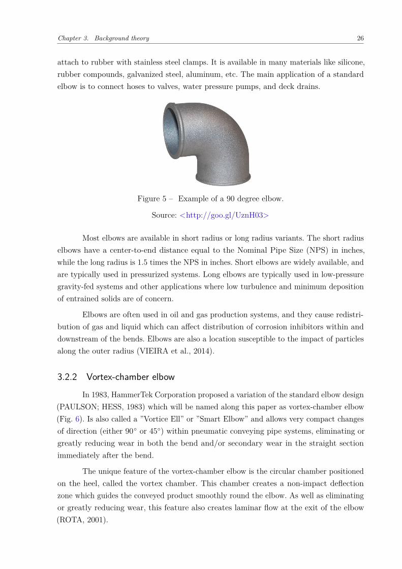
attach to rubber with stainless steel clamps. It is available in many materials like silicone,rubber compounds, galvanized steel, aluminum, etc. The main application of a standardelbow is to connect hoses to valves, water pressure pumps, and deck drains.
Figure 5 – Example of a 90 degree elbow.
Source: <http://goo.gl/UznH03>
Most elbows are available in short radius or long radius variants. The short radiuselbows have a center-to-end distance equal to the Nominal Pipe Size (NPS) in inches,while the long radius is 1.5 times the NPS in inches. Short elbows are widely available, andare typically used in pressurized systems. Long elbows are typically used in low-pressuregravity-fed systems and other applications where low turbulence and minimum depositionof entrained solids are of concern.
Elbows are often used in oil and gas production systems, and they cause redistri-bution of gas and liquid which can affect distribution of corrosion inhibitors within anddownstream of the bends. Elbows are also a location susceptible to the impact of particlesalong the outer radius (VIEIRA et al., 2014).
3.2.2 Vortex-chamber elbow
In 1983, HammerTek Corporation proposed a variation of the standard elbow design(PAULSON; HESS, 1983) which will be named along this paper as vortex-chamber elbow(Fig. 6). Is also called a ”Vortice Ell” or ”Smart Elbow” and allows very compact changesof direction (either 90 or 45) within pneumatic conveying pipe systems, eliminating orgreatly reducing wear in both the bend and/or secondary wear in the straight sectionimmediately after the bend.
The unique feature of the vortex-chamber elbow is the circular chamber positionedon the heel, called the vortex chamber. This chamber creates a non-impact deflectionzone which guides the conveyed product smoothly round the elbow. As well as eliminatingor greatly reducing wear, this feature also creates laminar flow at the exit of the elbow(ROTA, 2001).

Chapter 3. Background theory 27
Figure 6 – Example of a vortex-chamber elbow.
Source: <http://goo.gl/q26dxh>
Although not commonly found in daily life, will be shown during this work that forindustrial applications which require the transport of abrasive particles the vortex-chamberelbow provides an excellent alternative to the standard elbow.
3.3 CFD applied to erosion problemsMany efforts have motivated the research community to understand the physics be-
hind the erosion process in pipe systems. Experimental investigations (CHEN; MCLAURY;SHIRAZI, 2006; CHEN; MCLAURY; SHIRAZI, 2004; VIEIRA et al., 2014; TAKAHASHIet al., 2010; MAZUMDER; SHIRAZI; MCLAURY, 2008) support the development ofempirical correlations and models that are capable to predict the erosion behavior bothsingle and multiphase flows (AHLERT, 1994; NEILSON; GILCHRIST, 1968; OKA; OKA-MURA; YOSHIDA, 2005a; OKA; OKAMURA; YOSHIDA, 2005b; ZHANG et al., 2007).In this sense, progress in understanding the erosion due to particles has been achieved bythe utilization of CFD models that can accurately simulate the fluid and particle motionthrough pipelines and bends (LAíN; SOMMERFELD, 2013).
Four empirical models for the calculation of the erosion ratio were tested in thiswork. It should be noticed that these models are implemented in Unsteady Cyclone Flow3D (UNSCYFL3D), working alongside the fluid and particle models. These models arepresented below but only the Oka, Okamura e Yoshida (2005a) model was used to simulateall the cases. Oka, Okamura e Yoshida (2005a) will be explained in details in Section 4.3.
3.3.1 Erosion correlations
The erosion rate is defined as the mass of removed material per unit of area perunit of time. It is calculated on the walls by accumulating the damage each particle causes
Chapter 3. Background theory 28
when colliding against the wall surface. It is given by:
Ef = 1Af
∑π(f)
mπ er (3.1)
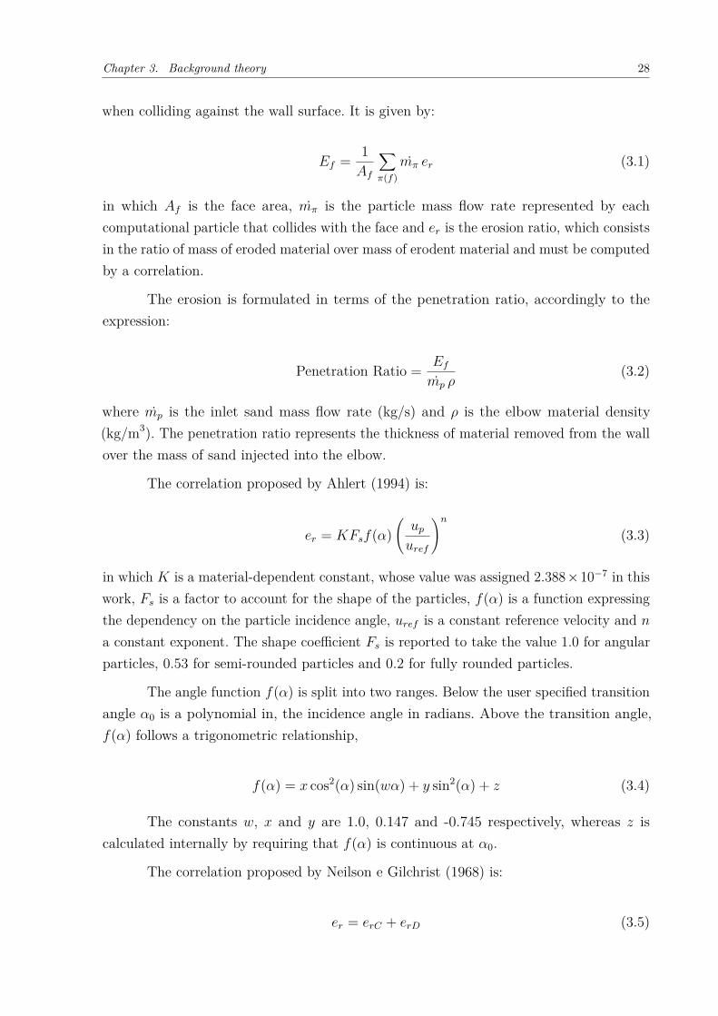
in which Af is the face area, mπ is the particle mass flow rate represented by eachcomputational particle that collides with the face and er is the erosion ratio, which consistsin the ratio of mass of eroded material over mass of erodent material and must be computedby a correlation.
The erosion is formulated in terms of the penetration ratio, accordingly to theexpression:
Penetration Ratio = Efmp ρ
(3.2)
where mp is the inlet sand mass flow rate (kg/s) and ρ is the elbow material density(kg/m3). The penetration ratio represents the thickness of material removed from the wallover the mass of sand injected into the elbow.
The correlation proposed by Ahlert (1994) is:
er = KFsf(α)(upuref
)n(3.3)
in which K is a material-dependent constant, whose value was assigned 2.388×10⁻⁷ in thiswork, Fs is a factor to account for the shape of the particles, f(α) is a function expressingthe dependency on the particle incidence angle, uref is a constant reference velocity and na constant exponent. The shape coefficient Fs is reported to take the value 1.0 for angularparticles, 0.53 for semi-rounded particles and 0.2 for fully rounded particles.
The angle function f(α) is split into two ranges. Below the user specified transitionangle α0 is a polynomial in, the incidence angle in radians. Above the transition angle,f(α) follows a trigonometric relationship,
f(α) = x cos2(α) sin(wα) + y sin2(α) + z (3.4)
The constants w, x and y are 1.0, 0.147 and -0.745 respectively, whereas z iscalculated internally by requiring that f(α) is continuous at α0.
The correlation proposed by Neilson e Gilchrist (1968) is:
er = erC + erD (3.5)
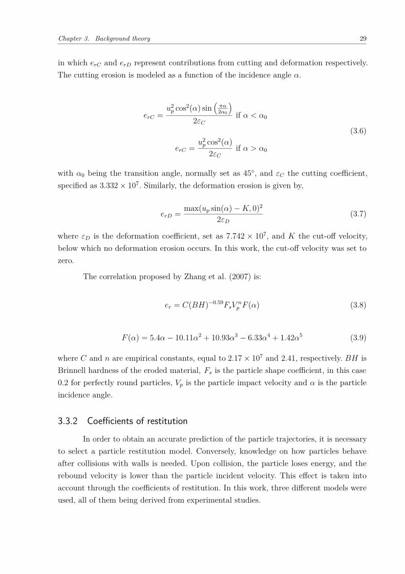
Chapter 3. Background theory 29
in which erC and erD represent contributions from cutting and deformation respectively.The cutting erosion is modeled as a function of the incidence angle α.
erC =u2p cos2(α) sin
(πα2α0
)2εC
if α < α0
(3.6)
erC =u2p cos2(α)
2εCif α > α0
with α0 being the transition angle, normally set as 45, and εC the cutting coefficient,specified as 3.332× 10⁷. Similarly, the deformation erosion is given by,
erD = max(up sin(α)−K, 0)2
2εD(3.7)
where εD is the deformation coefficient, set as 7.742 × 10⁷, and K the cut-off velocity,below which no deformation erosion occurs. In this work, the cut-off velocity was set tozero.
The correlation proposed by Zhang et al. (2007) is:
er = C(BH)−0.59FsVnp F (α) (3.8)
F (α) = 5.4α− 10.11α2 + 10.93α3 − 6.33α4 + 1.42α5 (3.9)
where C and n are empirical constants, equal to 2.17× 10⁷ and 2.41, respectively. BH isBrinnell hardness of the eroded material, Fs is the particle shape coefficient, in this case0.2 for perfectly round particles, Vp is the particle impact velocity and α is the particleincidence angle.
3.3.2 Coefficients of restitution
In order to obtain an accurate prediction of the particle trajectories, it is necessaryto select a particle restitution model. Conversely, knowledge on how particles behaveafter collisions with walls is needed. Upon collision, the particle loses energy, and therebound velocity is lower than the particle incident velocity. This effect is taken intoaccount through the coefficients of restitution. In this work, three different models wereused, all of them being derived from experimental studies.

Chapter 3. Background theory 30
The model proposed by Forder, Thew e Harrison (1998) for the normal and parallelcoefficients of restitution is given, respectively, by:
e = 0.988− 0.78α + 0.19α2 − 0.024α3 + 0.0027α4 (3.10)
epar = 1− 0.78α + 0.84α2 − 0.21α3 + 0.028α4 − 0.022α5 (3.11)
where α is the particle incidence angle in radians.
Sommerfeld e Huber (1999) proposed a model for the normal coefficient of restitutiononly, regarding the parallel component equal to one. The reason for that is the lowcontribution of the parallel component on the reflection of particles after collision. Thecorrelation for the normal restitution coefficient is given by:
e = max(1− 0.013α, 0.7) (3.12)
Despite the coefficients presented above the model proposed by Grant e Tabakoff(1975), which was not shown here, has a better accuracy due to its relation on experimentaldata on aluminum and sand. This model will also be presented in Section 4.3.
3.3.3 Coefficients of friction
Friction is not itself a fundamental force but arises from forces between the twocontacting surfaces. The complexity of these interactions makes the calculation of frictionfrom first principles impractical and necessitates the use of empirical methods for analysisand the development of theory.
An empirical model proposed by Sommerfeld e Huber (1999) described below:
µ = max(0.5− 0.175α, 0.15) (3.13)
It is worth noticing that the static and dynamic coefficients of friction were assumedto be equal in this work. No considerable difference was detected by prescribing the dynamiccoefficient lower than the static one.

31
4 Mathematical models
It is clear that many different simulations techniques are available for the present study.However not every technique is suitable for the type of flow being solved. Based on thetype of flow, assumptions can be made that simplify the flow equations. This leads to aset of equations that should resolve the flow field with sufficient accuracy while using thecomputational resources as effective as possible.
This chapter presents the mathematical models that should be sufficient for thecurrent study. For the gas phase solution the RANS method with a two-layer k-epsilonturbulence model is employed. The particulate phase is treated in a Lagrangian framework,having the equation of motion based on Newton’s second law. For the erosion calculationthe most accurate model is proposed and utilized. Every technique and model will bedetailed separately.
The chapter is structured as follows. First, Section 4.1 presents the flow equations.Then, Section 4.2 shows the particle motion equations. Finally, the employed erosion modelis presented in Section 4.3.
4.1 Gas phase equationsSimulations of fluids are based on the Navier Stokes Equations (NSE). In tensor
notation the continuity and Cauchy momentum equation are respectively,
∂ρ
∂t+ ∂(ρui)
∂xi= 0 (4.1)
∂(ρui)∂t
+ ∂(ρuiuj)∂xj
= − ∂p
∂xi+ ∂τij∂xj
+ fi (4.2)
where p is the pressure, ρ is the fluid density, ui represents the i component of the velocityvector, τij denotes the molecular viscous tensor and fi is the component i of the sourceterm.
For a Newtonian fluid, where ν represents the the kinematic viscosity of the fluid,the tensor is modeled with the Stokes model of viscous stress,
τij = ν
(∂ui∂xj
+ ∂uj∂xi
)− 2
3µδij (4.3)
Chapter 4. Mathematical models 32
For the present study, a steady-state and incompressible flow is assumed. Externalforces such as gravity forces and source terms due to phase interaction ( Suip) are addedto the momentum equation. Now the NSE for continuity and momentum are,
∂(ρui)∂xi
= 0 (4.4)
∂(ρuiuj)∂xj
= − ∂p
∂xi+ ∂
∂xj
[ν
(∂ui∂xj
+ ∂uj∂xi
)]+ Suip + ρgi (4.5)
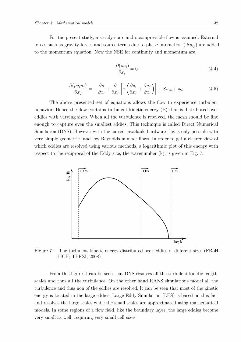
The above presented set of equations allows the flow to experience turbulentbehavior. Hence the flow contains turbulent kinetic energy (E) that is distributed overeddies with varying sizes. When all the turbulence is resolved, the mesh should be fineenough to capture even the smallest eddies. This technique is called Direct NumericalSimulation (DNS). However with the current available hardware this is only possible withvery simple geometries and low Reynolds number flows. In order to get a clearer view ofwhich eddies are resolved using various methods, a logarithmic plot of this energy withrespect to the reciprocal of the Eddy size, the wavenumber (k), is given in Fig. 7.
log k
log
E
RANS LES DNS
Figure 7 – The turbulent kinetic energy distributed over eddies of different sizes (FRöH-LICH; TERZI, 2008).
From this figure it can be seen that DNS resolves all the turbulent kinetic lengthscales and thus all the turbulence. On the other hand RANS simulations model all theturbulence and thus non of the eddies are resolved. It can be seen that most of the kineticenergy is located in the large eddies. Large Eddy Simulation (LES) is based on this factand resolves the large scales while the small scales are approximated using mathematicalmodels. In some regions of a flow field, like the boundary layer, the large eddies becomevery small as well, requiring very small cell sizes.
Chapter 4. Mathematical models 33
For the current study, a confined flow is considered. Since high Reynolds number ispresent and complex flow phenomena occur, DNS is not an option for solving the flow.LES is also discarded as an option due to its high computational costs. Since RANS usesthe least computational resources while still providing sufficiently accurate results, themain focus lies on this technique. The next section shows more detail about this method.
4.1.1 Reynolds Averaged Navier Stokes simulations
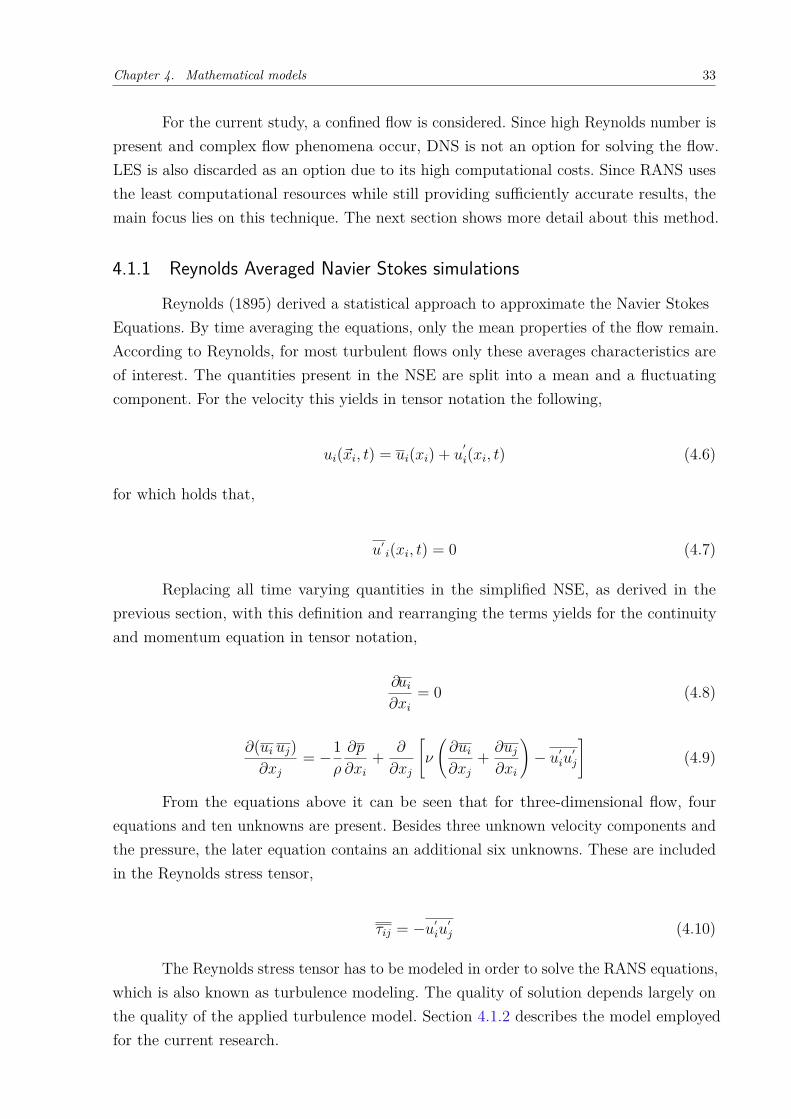
Reynolds (1895) derived a statistical approach to approximate the Navier StokesEquations. By time averaging the equations, only the mean properties of the flow remain.According to Reynolds, for most turbulent flows only these averages characteristics areof interest. The quantities present in the NSE are split into a mean and a fluctuatingcomponent. For the velocity this yields in tensor notation the following,
ui(~xi, t) = ui(xi) + u′
i(xi, t) (4.6)
for which holds that,
u′i(xi, t) = 0 (4.7)
Replacing all time varying quantities in the simplified NSE, as derived in theprevious section, with this definition and rearranging the terms yields for the continuityand momentum equation in tensor notation,
∂ui∂xi
= 0 (4.8)
∂(ui uj)∂xj
= −1ρ
∂p
∂xi+ ∂
∂xj
[ν
(∂ui∂xj
+ ∂uj∂xi
)− u′
iu′j
](4.9)
From the equations above it can be seen that for three-dimensional flow, fourequations and ten unknowns are present. Besides three unknown velocity components andthe pressure, the later equation contains an additional six unknowns. These are includedin the Reynolds stress tensor,
τij = −u′iu
′j (4.10)
The Reynolds stress tensor has to be modeled in order to solve the RANS equations,which is also known as turbulence modeling. The quality of solution depends largely onthe quality of the applied turbulence model. Section 4.1.2 describes the model employedfor the current research.

Chapter 4. Mathematical models 34
4.1.2 Turbulence model
The Reynolds stress tensor, τij, is often approximated by the Boussinesq (1877)hypothesis in order to link the Reynolds stresses with the mean velocity gradients. Thisapproximation is formulated as follows,
τij = −νt(∂ui∂xj
+ ∂uj∂xi
)+ 2
3kδij (4.11)
In this equation both the kinematic Eddy viscosity, νt and the turbulent kineticenergy, k, are unknown. Closure models provide a means to compute these extra quantitiesby introducing extra equations. The models can be classified into four different types;algebraic models, one equation models, two equation models and second order closuremodels. Thereof, according to Wilcox (1994), for RANS simulations the two equationmodels are the most popular. On the other hand, when a Detached Eddy Simulation(DES) simulation is performed, often a one equation model is employed. The term one ortwo equation turbulence model implies that one or two extra transport variables are usedfor the formulation that are related to νt and k.
For RANS simulations the best choice is to use the k − ε or the k − ω turbulencemodel. These models solve two extra transport equations. One for k and one for ε or ω.These extra variables relate to νt for the k − ε model as,
νt = Cµk2
ε(4.12)
and for k − ω as,
νt = k
ω(4.13)
For this dissertation, a variation of the k− ε is used and will be discussed in detailsin the following subsections.
4.1.2.1 Two layer k − ε model
The most famous model of the two is the k − ε model of which the standard isset by Jones e Launder (1972). In this formulation the second transport variable used isthe turbulent kinetic energy dissipation ε. In literature the method is often referred to asthe Standard k − ε model. When applying the Standard k − ε model, usually the closurecoefficients published in Launder e Sharma (1974) are used.
The two layer k − ε model is employed, as it can handle well both the core flowand the near wall region. Essentially, it consists in solving the standard model for theturbulent flow region and a one equation model for the region affected by the viscosity. In

Chapter 4. Mathematical models 35
the one equation k − ε model, the conservation equation for k is retained, whereas ε iscomputed from,
ε = k3/2
lε(4.14)
The length scale that appears in Eq. (4.14) is computed from,
lε = y Cl (1− e−Rey/Aε) (4.15)
In Eq. (4.15), Rey is the turbulent Reynolds number, defined as:
Rey = ρ y√k
µ(4.16)
where y is the distance from the wall to the element centers. This number is the demarcationof the two regions, fully turbulent if Rey > Re∗y, Re∗y = 200 and viscosity-affected,Rey < 200. For the one equation model, the turbulent viscosity is computed from,
µt,2layer = ρCµ lµ√k (4.17)
The length scale in the equation above is computed as below:
lµ = y Cl (1− e−Rey/Aµ) (4.18)
In UNSCYFL3D code, both the standard k−ε and the one equation model describedabove are solved over the whole domain, and the solutions for the turbulent viscosityand the turbulence kinetic energy dissipation rate provided by both models are smoothlyblended,
µt = λε µt,standard + (1− λε)µt,2layer (4.19)
A blending function, λε, is defined in such a way that it is equal to unity far fromwalls and is zero very near walls. The blending function used here is,
λε = 12
[1 + tanh
(Rey −Re∗y
A
)](4.20)
The constant A determines the width of the blending function,
A =0.20Re∗y
artanh (0.98) (4.21)

Chapter 4. Mathematical models 36
The purpose of the blending function λε is to prevent solution divergence when thesolution from both the standard and the one-equation models do not match. The constantsin the length scale formulas, Eqs. (4.15) and (4.18), are taken from:
Cl = 0.4187C−3/4µ Aµ = 70 Aε = 2Cl (4.22)
Since no wall-functions are used, it is very important to refine the grid so as tohave y+ < 1 in the first element away from the wall and ensure accurate results for thefluid flow.
4.2 Particle motion equationsAs mentioned in Section 4, the dispersed phase is treated in a Lagrangian framework,
in which each particle is tracked through the domain and its equation of motion is based onNewton’s second law. The trajectory, linear momentum and angular momentum equationsfor a rigid, spherical particle can be written, respectively,
dxpidt
= upi (4.23)
mpdupidt
= mp3ρCD4ρpdp
(ui − upi) + Fsi + Fri +(
1− ρ
ρp
)mpgi (4.24)
Ipdωpidt
= Ti (4.25)
In the above equations, ui = Ui + u′i are the components of the instantaneous fluid
velocity. The average fluid velocity Ui is interpolated from the resolved flow field, whereasthe fluctuating component u′
i is calculated according to the Langevin dispersion modelproposed by Sommerfeld (2001). dp is the particle diameter and Ip = 0.1mp d
2p is the
moment of inertia for a sphere. Unlike most commercial CFD codes, UNSCYFL3D solvesfor the particle rotation. This is particularly important when dealing with large particles,which frequently collide with walls.
The empirical correlation proposed by Schiller e Naumann (1935) is used to evaluatethe drag coefficient past each particle:
CD = 24Re−1p (1 + 0.15Re0.687
p ) if Rep < 1000
(4.26)
CD = 0.44 if Rep > 1000

Chapter 4. Mathematical models 37
In Eqs. (4.26), Rep is the particle Reynolds number Rep = ρ dp|~u− ~up|/µ.
The calculation of the shear-induced lift force is based on the analytical resultof Saffman (1965) and extended for higher particle Reynolds numbers according to Mei(1992):
~Fs = 1.615 dpRe1/2s Cls[(~u− ~up)× ~ω] (4.27)
~ω is the vorticity, Res = ρ d2p |~ω|/µ is the particle Reynolds number of the shear flow and
Cls = Fls/Fls,Saff represents the ratio of the extend lift force to the Saffman force:
Cls = (1− 0.3314 β0.5)e−0.1Rep + 0.3314 β0.5 if Rep < 40
(4.28)
Cls = 0.0524(β Rep)0.5 if Rep > 40
β is a parameter β = 0.5Res/Rep which varies with 0.005 < β < 0.4.
The rotation-induced lift is computed based on the relation given by Rubinow eKeller (1961), which was extended to account for the relative motion between particle andfluid:
~Fr = π
8 ρ d3p
RepRer
Clr[~Ω× (~u− ~up)]
|~Ω|(4.29)
In Eq. (4.29), ~Ω = 0.5 ~∇× ~u− ~ωp and Res = ρ d2p |~Ω|/µ. The lift coefficient Clr is
obtained from the correlation proposed by Lun e Liu (1997):
Clr = RerRep
if Rep < 1
(4.30)
Clr = RerRep
(0.178 + 0.822Re−0.522p ) if Rep > 1
Also, the rotating particle experiences torque from the fluid flow. The correlationof Rubinow e Keller (1961) was extended to account for the relative motion between fluidand particle at higher Reynolds number:
~T = Crρ d5
p
64 |~Ω| ~Ω (4.31)
The coefficient of rotation, Cr, was obtained from the following correlation, derivedfrom and the direct numerical simulations of Dennis, Singh e Ingham (1980):
Chapter 4. Mathematical models 38
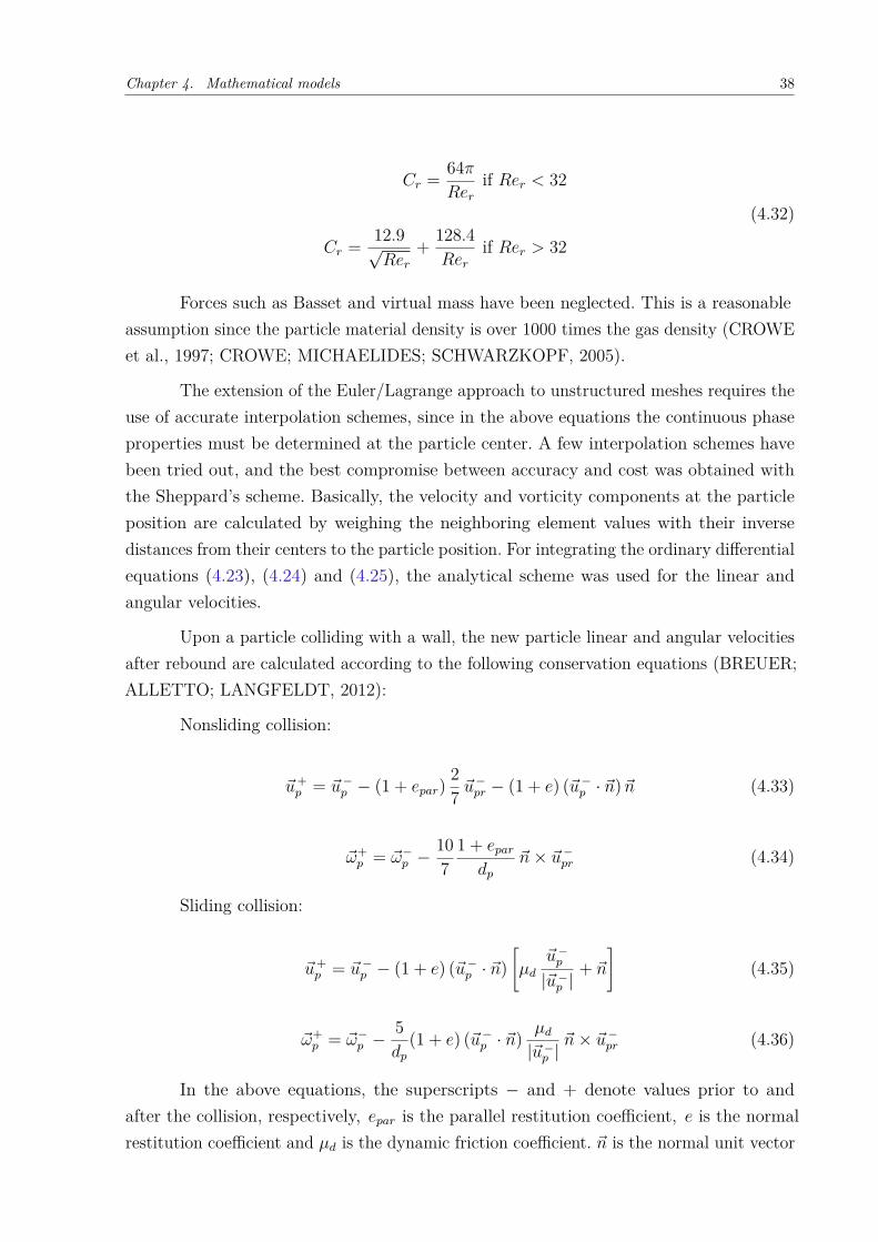
Cr = 64πRer
if Rer < 32
(4.32)
Cr = 12.9√Rer
+ 128.4Rer
if Rer > 32
Forces such as Basset and virtual mass have been neglected. This is a reasonableassumption since the particle material density is over 1000 times the gas density (CROWEet al., 1997; CROWE; MICHAELIDES; SCHWARZKOPF, 2005).
The extension of the Euler/Lagrange approach to unstructured meshes requires theuse of accurate interpolation schemes, since in the above equations the continuous phaseproperties must be determined at the particle center. A few interpolation schemes havebeen tried out, and the best compromise between accuracy and cost was obtained withthe Sheppard’s scheme. Basically, the velocity and vorticity components at the particleposition are calculated by weighing the neighboring element values with their inversedistances from their centers to the particle position. For integrating the ordinary differentialequations (4.23), (4.24) and (4.25), the analytical scheme was used for the linear andangular velocities.
Upon a particle colliding with a wall, the new particle linear and angular velocitiesafter rebound are calculated according to the following conservation equations (BREUER;ALLETTO; LANGFELDT, 2012):
Nonsliding collision:
~u+p = ~u−p − (1 + epar)
27 ~u
−pr − (1 + e) (~u−p · ~n)~n (4.33)
~ω+p = ~ω−p −
107
1 + epardp
~n× ~u−pr (4.34)
Sliding collision:
~u+p = ~u−p − (1 + e) (~u−p · ~n)
[µd
~u−p|~u−p |
+ ~n
](4.35)
~ω+p = ~ω−p −
5dp
(1 + e) (~u−p · ~n) µd|~u−p |
~n× ~u−pr (4.36)
In the above equations, the superscripts − and + denote values prior to andafter the collision, respectively, epar is the parallel restitution coefficient, e is the normalrestitution coefficient and µd is the dynamic friction coefficient. ~n is the normal unit vector
Chapter 4. Mathematical models 39
pointing outwards of the element face being impacted. ~urp is the relative velocity at thecontact point:
~upr = ~up − (~up · ~n)~n+ dp2 ωp × ~n (4.37)
Inter-particle collisions are modeled with a stochastic, hard-sphere model. Asdescribed by Oesterle e Petitjean (1993) and Sommerfeld (2001), for each computationalparticle, a fictitious collision partner is generated, and the probability of a collision ischecked based on an analogy with kinetic theory of gases. This in turn requires that theaverage and RMS linear and angular velocities, as well as the particle concentration in eachcontrol volume, be sampled and stored every Lagrangian calculation. Although demandinga lot of memory, the method is rather economical and effective, and avoids the use of adeterministic collision model, which is quite expensive computationally.
Numerous experimental studies have shown evidence that wall roughness is impor-tant in the particle behavior. Therefore, their influence must be included in the modeling.As demonstrated by Lain, Sommerfeld e Kussin (2002) and Benson, Tanaka e Eaton (2004),the wall roughness plays a vital role in the dispersion of particles in pneumatic transportsystems. In order to account for such effects, we implemented the model proposed bySommerfeld e Huber (1999), to represent the effects of surface asperities on the particle flow.In summary, the wall roughness is simulated by assuming that the effective impact angleαgeometric is composed of the geometric impact angle α geometric added to a stochasticcontribution due to wall roughness.
α = αgeometric + ξ ·∆γ (4.38)
This stochastic contribution is sampled from a Gaussian distribution with a stan-dard deviation ∆γ, which depends on the structure of wall roughness and particle size.Unfortunately, the value of ∆γ must be calibrated so as to provide the best agreementbetween the experimental and simulated pressure losses.
When a structured grid is used, it is simple to determine the element hosting theparticle, as there exists a straightforward relationship between the element index and itsphysical location. Because an unstructured grid is used in this work, there is the needfor a specific algorithm to locate the particle after its final position is calculated by theintegration of Eq. (4.23). For that purpose, the particle-localization algorithm proposedby Haselbacher, Najjar e Ferry (2007) is used and will be detailed in Section 6.
Chapter 4. Mathematical models 40
4.3 Erosion prediction equationAfter a exhaustive search in literature, the works from Pereira, Souza e Moro
(2014) and Duarte, Souza e dos Santos (2015) showed that the combination of the modelsproposed by Oka, Okamura e Yoshida (2005b) for the erosion ratio and Grant e Tabakoff(1975) for the coefficient of restitution were the most suitable for the erosion predictionwhen ninety-degree-elbows are investigated. Accordingly, these models were used in thiswork and will be described below.
As previously explained, the erosion rate and the penetration ratio are defined,respectively, as:
Ef = 1Af
∑π(f)
mπ er (4.39)
Penetration Ratio = Efmp ρ
(4.40)
The predictive equation for erosion damage proposed by Oka, Okamura e Yoshida(2005b) can be expressed as:
E(α) = g(α)E90 (4.41)
E(α) and E90 denote a unit of eroded material per mass of particles (mm3kg−1). g(α) isthe impact angle dependence expressed by two trigonometric functions and by the initialeroded material Vickers hardness number (Hv) in unit of GPa, as in Eq. (4.42):
g(α) = (sinα)n1(1 + Hv (1− sinα))n2 (4.42)
n1 and n2 are exponents determined by the eroded material hardness and other impactconditions such particle properties and shape. These exponents shows the effects of repeatedplastic deformation and cutting action, and for particles of SiO2-1 are expressed by:
n1 = 0.71 (Hv)0.14 (4.43)
n2 = 2.4 (Hv)−0.94 (4.44)
The reference erosion ratio E90 (erosion damage at normal impact angle) is relatedto impact velocity, particle diameter and eroded material hardness, and can be expanded

Chapter 4. Mathematical models 41
as follows:
E90 = K (aHv)k1b
(upuref
)k2 ( Dp
Dref
)k3
(4.45)
u and D are the impact velocity (m s−1) and particle diameter (µm), respectively, anduref and Dref are the reference impact velocity and the particle diameter used in theexperiments by Oka, Okamura e Yoshida (2005b). k3 is a exponent which take an arbitraryunit and is determined by the properties of the particle. k2 exponent can be determinedby eroded material Vickers hardness and by particle properties, as shown in Eq. (4.46):
k2 = 2.3 (Hv)0.038 (4.46)
According to Oka, Okamura e Yoshida (2005b) the term K (aHv)k1b is highlydependent on the type of the particle and eroded material Vickers hardness which arenot correlated with the impact conditions and other factors. The present work used theexperimental data from Oka, Okamura e Yoshida (2005b) to derive a function and obtainthe relationship between eroded material Vickers hardness and E90 at the reference impactvelocity. The function obtained by the curve fitting shown in Fig. 2 of Oka, Okamura eYoshida (2005b) for the pair SiO2-aluminum is provided below::
K (aHv)k1b ≈ 81.714 (Hv)−0.79 (4.47)
Is important to emphasize that this function is for the pair sand-aluminum andmay change for other materials. As a result, E90 can be expressed as follows:
E90 = 81.714 (Hv)−0.79(upuref
)k2 ( Dp
Dref
)k3
(4.48)
The purported strength of the Oka model is that the coefficients for a particularcombination of eroded and erodent materials can be derived from more fundamentalcoefficients. Hence, the fundamental coefficients for sand can serve as a basis for bothsand-steel erosion and sand-aluminum erosion, for instance. Table 1 summarizes all theerosion ratio model constants used in the present work.
Grant e Tabakoff (1975) proposed the restitution model after treating the postcollisional particle movement dynamics in a statistical approach. Based on experimentaldata on aluminum and sand, they proposed equations (4.49) and (4.50) for the coefficients:
e = 0.993− 1.76α + 1.56α2 − 0.49α3 (4.49)

Chapter 4. Mathematical models 42
epar = 0.998− 1.55α + 2.11α2 − 0.67α3 (4.50)
Friction is another important effect to be accounted for in particle-wall interactions.Depending on the static and dynamic coefficients, particles can lose energy and velocity,directly affecting the erosion. In UNSCYFL3D, the standard coefficient was used (µ = 0.25).
Table 1 – Constants used for the erosion ratio correlation.
Eroded material type Aluminum (6061-T6)Eroded material Vickers hardness (Hv) 1.049GpaParticle type Angular SiO2-1Reference impact velocity (uref ) 104m/sReference particle diameter (Dref ) 326µmk2 2.3042k3 0.19n1 0.7148n2 2.2945
43
5 Finite volume discretization
For the current research the UNSCYFL3D code is employed. UNSCYFL3D, amongstmany other CFD packages, uses a Finite Volume Method (FVM) in order to resolve a flowfield depending on its geometrical boundaries and their respective boundary conditions.For this approach the equations presented in the previous chapter have to be discretizedin space. Since the problems is treated in a steady-state form, the discretization in timewill not be described in this work.
This chapter presents a brief overview of the discretization methods employed forthe current research. It is largely based on the information in the Fluent Guide (2005),supplemented with the work of Ferziger e Peric (2002) and Mathur e Murthy (1997). Themethods outlined below may not be optimal, but they have proven to deliver sufficientlyaccurate results within a reasonable amount of time for the problem at hand.
Section 5.1 introduces the FVM. Then Sections 5.2 present the spatial discretization.The pressure-velocity coupling is presented in Section 5.3 and the solution procedure iselaborated in Section 5.4.
5.1 Finite Volume MethodThe Finite Volume Method (FVM) is a method for representing and evaluating
partial differential equations in the form of algebraic equations (LEVEQUE, 2002; TORO,2009). Similar to the finite difference method or finite element method, values are calculatedat discrete places on a meshed geometry. In the finite volume method, volume integralsin a partial differential equation that contain a divergence term are converted to surfaceintegrals, using the divergence theorem. These terms are then evaluated as fluxes at thesurfaces of each finite volume. Because the flux entering a given volume is identical tothat leaving the adjacent volume, these methods are conservative. Another advantage ofthe finite volume method is that it is easily formulated to allow for unstructured meshes(VERSTEEG; MALALASEKERA, 2007).
5.2 Spatial discretizationThe conservation equations for the continuity, velocity components and for the
turbulence variables in steady state can be written generically as:
∂
∂xj(ρujφ) = ∂
∂xj
(Γ ∂φ
∂xj
)+ Sφ (5.1)
Chapter 5. Finite volume discretization 44
By integrating the general conservation Eq. 5.1 over the control volume V , weobtain:
∮Aρφ~V · d ~A =
∮A
Γgradφ · d ~A+∮VSφdV (5.2)
Note that, for the terms involving surface integrals in Eq. 5.2, the Gauss DivergenceTheorem was applied to convert the volume integrals into surface integrals (FERZIGER;PERIC, 2002):
∫V
∂φ
∂xidV =
∮Aφ~li · d ~A (5.3)
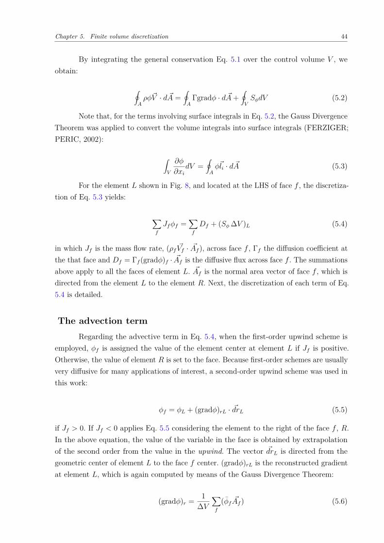
For the element L shown in Fig. 8, and located at the LHS of face f , the discretiza-tion of Eq. 5.3 yields:
∑f
Jfφf =∑f
Df + (Sφ ∆V )L (5.4)
in which Jf is the mass flow rate, (ρf ~Vf · ~Af ), across face f , Γf the diffusion coefficient atthe that face and Df = Γf (gradφ)f · ~Af is the diffusive flux across face f . The summationsabove apply to all the faces of element L. ~Af is the normal area vector of face f , which isdirected from the element L to the element R. Next, the discretization of each term of Eq.5.4 is detailed.
The advection termRegarding the advective term in Eq. 5.4, when the first-order upwind scheme is
employed, φf is assigned the value of the element center at element L if Jf is positive.Otherwise, the value of element R is set to the face. Because first-order schemes are usuallyvery diffusive for many applications of interest, a second-order upwind scheme was used inthis work:
φf = φL + (gradφ)rL · ~drL (5.5)
if Jf > 0. If Jf < 0 applies Eq. 5.5 considering the element to the right of the face f , R.In the above equation, the value of the variable in the face is obtained by extrapolationof the second order from the value in the upwind. The vector ~drL is directed from thegeometric center of element L to the face f center. (gradφ)rL is the reconstructed gradientat element L, which is again computed by means of the Gauss Divergence Theorem:
(gradφ)r = 1∆V
∑f
(φf ~Af ) (5.6)

Chapter 5. Finite volume discretization 45
L
R
f
Af
drR
drL
ds
Figure 8 – Control volume for a finite volume discretization.
where φf is the average of φ the element centers sharing face f .
The first term on the right side of Eq. 5.6 is always implicitly treated, whereas thesecond term is treated as source term and therefore calculated explicitly.
The diffusion termIt can be proven that the diffusive flux for face f is given by (MATHUR; MURTHY,
1997):
Df = Γf(φR − φL)| ~ds|
~Af · ~Af~Af · ~es
+ Γf
gradφ · ~Af − gradφ · ~es~Af · ~Af~Af · ~es
(5.7)
In Eq. 5.7, ~es is the unit vector connecting the centers of elements R e L, ~es = ~ds
| ~dr| .The first term at the RHS of Eq. 5.7 is treated implicitly, whereas the remaining terms,which represent the secondary diffusion, are calculated explicitly and therefore incorporatedinto the source-term S in Eq. 5.4. The secondary diffusion is null for hexahedra for instance,because vectors ~Af and ~es are collinear. The gradient at face f , gradφ, is calculated asthe average of the gradients at the adjacent elements. The treatment above is equivalentto the application of the second-order, centered differencing scheme in structured meshesand is advantageous in the sense that it does not depend on the element shape.
5.3 Pressure-velocity couplingSo far, it was proved that the momentum equations can be discretized via finite
volume in unstructured meshes. Note that the set of Eqs. 4.1 and 4.2 forms a system offour equations (continuity, momentum for u, v and w) and four unknowns (u, v, w and

Chapter 5. Finite volume discretization 46
p), thereby forming a given system. The velocity components must be determined by therespective conservation equations, but restricted with the imposed continuity. There is noexplicit equation for the pressure, which requires the deduction of an equation for thisvariable so a segregated method of solution can be employed. The UNSCYFL3D uses theSIMPLE method (Semi-Implicit Pressure-Linked Equations, (FERZIGER; PERIC, 2002))to generate this equation and ensure that the continuity equation is also satisfied.
In the SIMPLE method, the procedure solution of the equations for u, v, w andp is said segregated, which means that a system of linear equations for each of thesevariables are resolved independently by linear system solution methods, and sequentially.The process is repeated until all the standard equations residues is reduced until thespecified tolerance. Several global iterations, with the solution of linear systems for u, v, wand p, may be necessary due to the nonlinear nature of the Navier-Stokes equations andthe coupling between the variables. Since the variables converge at different speeds, it isnecessary under-relaxed the system solutions. For the case of transient problems, globaliterations should be performed at each time step, and the process is repeated at each timestep.
A more detailed discussion on pressure-velocity coupling can be found in (FERZIGER;PERIC, 2002).
5.4 Solution procedureFor the current study, only steady simulations are performed. For steady simulations
the SIMPLE algorithm by Patankar (1980) is employed and briefly discussed below.
The SIMPLE algorithm can be summarized as follows:
1. Start-up the values of the velocities components and pressure in the elements andthe mass flow rates across the faces of the calculation area, including the boundaries.These fields do not necessarily satisfy the conservation equations;
2. solves the linear system of equations for each component of the velocity vector, thiscorresponds to the predictor step. UNSCYFL3D uses biconjugated gradient method;
3. with the predicted velocity field, the mass flow rates is calculated on the faces of allthe elements. It is then solved the linear system for the pressure correction. Normally,it is necessary to use an efficient solver based on multigrid methods, for example;
4. by knowing the pressure correction, the mass flow rates are corrected on the faces,the pressure in each element, and the velocity components in each element;
5. evaluate the residues and the momentum equations after the corrector step andif they are satisfied according to the tolerance specified by the user, declares the
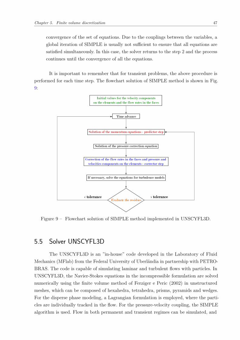
Chapter 5. Finite volume discretization 47
convergence of the set of equations. Due to the couplings between the variables, aglobal iteration of SIMPLE is usually not sufficient to ensure that all equations aresatisfied simultaneously. In this case, the solver returns to the step 2 and the processcontinues until the convergence of all the equations.
It is important to remember that for transient problems, the above procedure isperformed for each time step. The flowchart solution of SIMPLE method is shown in Fig.9:
Initial values for the velocity components
on the elements and the flow rates in the faces
Time advance
Solution of the momentum equations - predictor step
Correction of the flow rates in the faces and pressure and
velocities components on the elements - corrector step
If necessary, solve the equations for turbulence models
Solution of the pressure correction equation
Evaluate the residues> tolerance< tolerance
Figure 9 – Flowchart solution of SIMPLE method implemented in UNSCYFL3D.
5.5 Solver UNSCYFL3DThe UNSCYFL3D is an ”in-house” code developed in the Laboratory of Fluid
Mechanics (MFlab) from the Federal University of Uberlândia in partnership with PETRO-BRAS. The code is capable of simulating laminar and turbulent flows with particles. InUNSCYFL3D, the Navier-Stokes equations in the incompressible formulation are solvednumerically using the finite volume method of Ferziger e Peric (2002) in unstructuredmeshes, which can be composed of hexahedra, tetrahedra, prisms, pyramids and wedges.For the disperse phase modeling, a Lagrangian formulation is employed, where the parti-cles are individually tracked in the flow. For the pressure-velocity coupling, the SIMPLEalgorithm is used. Flow in both permanent and transient regimes can be simulated, and
Chapter 5. Finite volume discretization 48
6 boundary conditions can be prescribed: imposed velocity, symmetry, outflow, non-slip,imposed pressure and frequency.
The diffusive terms are discretized by 2nd order centered differences, for the advectiveterms, the upwind scheme and the 1st order centered scheme or upwind scheme 2nd ordercan be combined. The large scale turbulence models are: Smagorinsky, dynamic andYakhot. The SST and DES-SST models are also available. For the integration of themotion equations of the particles, it uses the analytical model previous described in Section4.2. Particles can be injected into faces in which the boundary condition of imposed velocityis applied. The following boundary conditions for the particles are possible: reflection,escape and frequency.
For the erosion-related problems the correlations from: Ahlert (1994), Neilsone Gilchrist (1968), Zhang et al. (2007) and Oka, Okamura e Yoshida (2005b) can beemployed. The coefficients of restitution can be selected from: Forder, Thew e Harrison(1998), Sommerfeld e Huber (1999) and Grant e Tabakoff (1975) models.
For time advance of the flow equations, the implicit Euler scheme 1st and threelevels in time 2nd can be used. The mesh converter was developed in C language, and thesolver in FORTRAN 90 language. Both flow and particles can be post processed usingParaview and VisIt tools.

49
6 Particle phase algorithm
According to Elghobashi (1993), when starting a single-phase flow into a flow witha high particle loading, four different regimes will be achieved, and these arrangementsrelate to the manner in which the flow "feels" the presence of the dispersed phase (type ofcoupling) and the manner in which the dispersed phase interferes with the turbulence ofthe continuous phase (attenuating or increasing the turbulence levels).
For both Lagrangian and Eulerian approaches, it should be noted that the two-waycoupling requires the description of the coupling between the phases and the particle.This interaction occurs through the tension between the phases at the particle surface. Inparticular, the coupling strength between the phases is the force acting on a single particledue to pressure and viscous tension caused by the disturbed fluid around. This force isequal in magnitude and opposite in direction to hydrodynamic force of the particle actingon the continuous phase. The coupling strength between the phases is the hydrodynamicforces on the surface less the contributions of the tensions of the undisturbed fluid ( e.g.,less forces due to the pressure gradients which occur regardless of the presence of theparticle).
The next section will briefly explain the coupling procedure used in UNSCYFL3D.
6.1 Coupling procedureThe coupled solution of the continuous and particle phases is summarized as follows
(LAíN; SOMMERFELD, 2012): first the steady-state solution for the fluid phase withoutparticles is computed. Subsequently, particles are injected and tracked throughout thedomain. For each control volume, the average and RMS linear and angular velocities, theparticle concentration and the source-terms for the fluid momentum equation are stored.
After all the particles have left the domain, the fluid flow is solved again, nowconsidering the source-terms sampled during the previous particle calculation. This processis repeated, taking the particle-to-particle collision into account, until a converged solutionfor both phases is reached. It is important to bear in mind that the particle statisticsmust be corrected during each particle calculation. Another important detail is that theparticle source term must be under-relaxed, for achieving convergence. The present workused 0.1 as under-relaxation factor for all the cases, and the quality of convergence wasmeasured based on the standard deviation of average velocities, which should be close to0.001. Normally, 100 coupling iterations are sufficient for convergence of both phases. Adetailed information about this method is given by (LAíN; SOMMERFELD, 2013).

Chapter 6. Particle phase algorithm 50
The scheme of this procedure is presented in Fig. 10.
Gridxgeneration,
Boundaryxconditions,
Inletxconditions
Eulerian Part
Calculationxofxthexfluidxflowxwithout
particlexphasexsourcexterms
Lagrangian Part
Trackingxofxparcels
withoutxinter-particlexcollisions,
Samplingxofxparticlexphasexproperties
andxsourcexterms
Eulerian Part
Calculationxofxthexfluidxflowxwith
particlexphasexsourcexterms:
-xConvergedxsolution
-xSolutionxwithxaxfixedxnumerxofxiterations
Lagrangian Part
Trackingxofxparcels
Samplingxofxparticlexphase
propertiesxandxsourcexterms
Lagrangian Part
Trackingxofxparcelsxwith
inter-particlexcollisions,
Samplingxofxparticlexphase
propertiesxandxsourcexterms
Convergence
Euler-Lagrange
coupling
Output:
Flowxfield
Particle-phasexstatistics
Couplingxiterations
withxsourcexterm
under-relaxation
Two-way Four-way
No
Yes
Figure 10 – Flow chart of fully coupled Euler-Lagrange calculations (LAíN; SOMMER-FELD, 2013).
To solve the differential equations, it is important to know the location of eachparticle within the Eulerian mesh. This occurs because to calculate the variation of velocityand position of the particles is necessary to interpolate the fluid properties to the positionof its center of mass. Usually, the computational determination of the cell in which aparticle is can be done quickly and efficiently by using a particle locator and a meshmapping in cartesian uniform meshes. However, this approach can not be directly used inunstructured grids (PENG et al., 2009), making the particle tracking problem an importantelement. Next section is dedicated to briefly explain the particle-location algorithm usedin the present report.

Chapter 6. Particle phase algorithm 51
6.2 Particle-tracking algorithmThe UNSCYFL3D code uses the algorithm proposed by Haselbacher, Najjar e
Ferry (2007). This choice was due to some specific features of this algorithm:
• this algorithm is robust enough to allow a particle to crosses more than one com-putational cell in a single step and time, in other words, the algorithm enables theparticle to go through long distances, which is a limiting factor for a number ofalgorithms;
• the algorithm is based on distances intersection rather than time intersection, whichis much more natural, once the particle tracking problem should be primarily aspatial problem, not temporal;
• the algorithm can be applied to Eulerian meshes consisting of polyhedral elements;
• according to the author, this algorithm is faster and more efficient than otherpublished algorithms.
The complete procedure of particle-location as well as the algorithms used are notpresented here because it differ completely from the main theme of the dissertation. Adetailed information about the algorithm and its implementation can be found in thepublication of Haselbacher, Najjar e Ferry (2007).
All the information presented until now allow the reader to familiarize themselveswith the problem analyzed and the procedure used for its solution. With this in mind, willbe presented in the following chapters the numerical setup and procedure (Chap. 7) andthe results (Chap. 8) obtained, respectively.

52
7 Numerical setup and procedure
According to the experiment configuration described by Mazumder, Shirazi eMcLaury (2008), which aluminum elbow specimens were used, sand particles were injectedin the horizontal line at about 1.22meters below the test piece. The test piece was a 90
elbow with a diameter of 0.0254meters (D) and a curvature radius of 0.0381meters. Theerosion profile were measured along the outer bend surface as shown in Fig. 11. Hence acomparison of the calculations with the measurements is also made for this location. Inorder to represent more realistic behavior at the specimen location, wthe hole domain wasincluded on the calculation, attempting to better reproduce the experimental conditions.
D
48D
1.5D
Flow
0°
90°
45°
22.5°
67.5°
Erosion region analysed
g
Figure 11 – Schematics of the elbow investigated.
At the inlet of the pipe, the fluid is injected with a mean conveying velocity of34.1m/s and a turbulence intensity of 5%. At the pipe walls a no-slip condition is appliedwhilst at the pipe exit an outlet condition is adopted. Table 2 summarize all the propertiesof the fluid, particle and pipe used in all computations. These conditions yield a pipeReynolds number of 5.93 × 10⁴ and a particle Stokes number based on the averageddiameter of 3.66.
Regarding the two-phase flow simulations, the mass loading ratio considered inthe experimental measurements was φ = 0.013. After the validation for the experimentalmass loading, higher mass loadings computations were carried out in order to quantifyits effect in the flow and in the penetration ratio. For all cases studied, the mean particlediameter was 182µm and the pipe material was Aluminum (6061-T6). The pipe wall
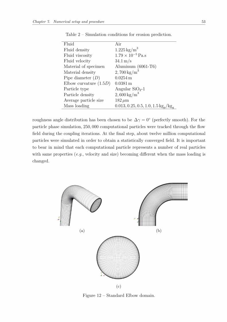
Chapter 7. Numerical setup and procedure 53
Table 2 – Simulation conditions for erosion prediction.
Fluid AirFluid density 1.225 kg/m3
Fluid viscosity 1.79× 10⁻⁵ Pa.sFluid velocity 34.1m/sMaterial of specimen Aluminum (6061-T6)Material density 2, 700 kg/m3
Pipe diameter (D) 0.0254mElbow curvature (1.5D) 0.0381mParticle type Angular SiO2-1Particle density 2, 600 kg/m3
Average particle size 182µmMass loading 0.013, 0.25, 0.5, 1.0, 1.5 kgp/kgg
roughness angle distribution has been chosen to be ∆γ = 0 (perfectly smooth). For theparticle phase simulation, 250, 000 computational particles were tracked through the flowfield during the coupling iterations. At the final step, about twelve million computationalparticles were simulated in order to obtain a statistically converged field. It is importantto bear in mind that each computational particle represents a number of real particleswith same properties (e.g., velocity and size) becoming different when the mass loading ischanged.
(a) (b)
(c)
Figure 12 – Standard Elbow domain.
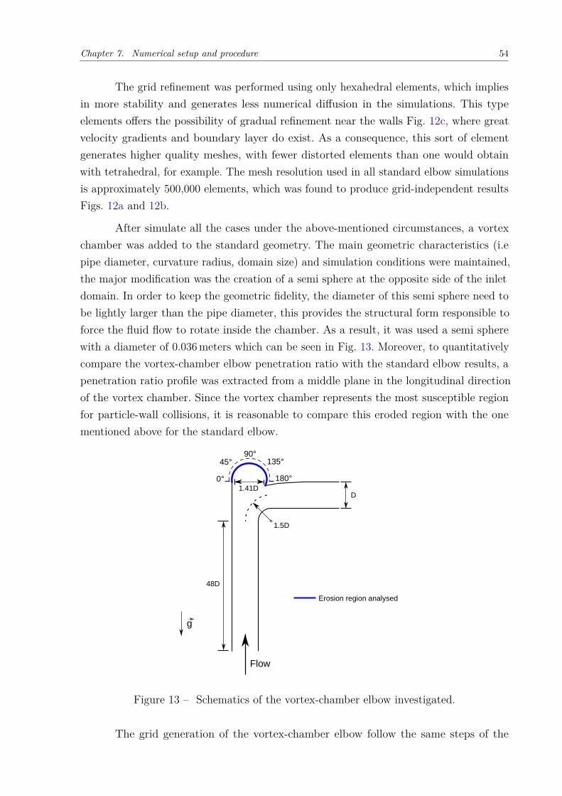
Chapter 7. Numerical setup and procedure 54
The grid refinement was performed using only hexahedral elements, which impliesin more stability and generates less numerical diffusion in the simulations. This typeelements offers the possibility of gradual refinement near the walls Fig. 12c, where greatvelocity gradients and boundary layer do exist. As a consequence, this sort of elementgenerates higher quality meshes, with fewer distorted elements than one would obtainwith tetrahedral, for example. The mesh resolution used in all standard elbow simulationsis approximately 500,000 elements, which was found to produce grid-independent resultsFigs. 12a and 12b.
After simulate all the cases under the above-mentioned circumstances, a vortexchamber was added to the standard geometry. The main geometric characteristics (i.epipe diameter, curvature radius, domain size) and simulation conditions were maintained,the major modification was the creation of a semi sphere at the opposite side of the inletdomain. In order to keep the geometric fidelity, the diameter of this semi sphere need tobe lightly larger than the pipe diameter, this provides the structural form responsible toforce the fluid flow to rotate inside the chamber. As a result, it was used a semi spherewith a diameter of 0.036meters which can be seen in Fig. 13. Moreover, to quantitativelycompare the vortex-chamber elbow penetration ratio with the standard elbow results, apenetration ratio profile was extracted from a middle plane in the longitudinal directionof the vortex chamber. Since the vortex chamber represents the most susceptible regionfor particle-wall collisions, it is reasonable to compare this eroded region with the onementioned above for the standard elbow.
D
48D
1.5D
Flow
Erosion region analysed
g
0°
90°
180°
45° 135°
1.41D
Figure 13 – Schematics of the vortex-chamber elbow investigated.
The grid generation of the vortex-chamber elbow follow the same steps of the

Chapter 7. Numerical setup and procedure 55
standard elbow. The grid refinement near the walls was preserved Fig. 14c, as well as theless distorted elements inside the vortex chamber Fig. 14b. To easily generate the vortexchamber mesh, an multi-block structured grid with an O-type structure composed of 5blocks was used resulting in a total of 670,000 hexahedral control volumes.
(a) (b)
(c)
Figure 14 – Vortex-Chamber Elbow domain.
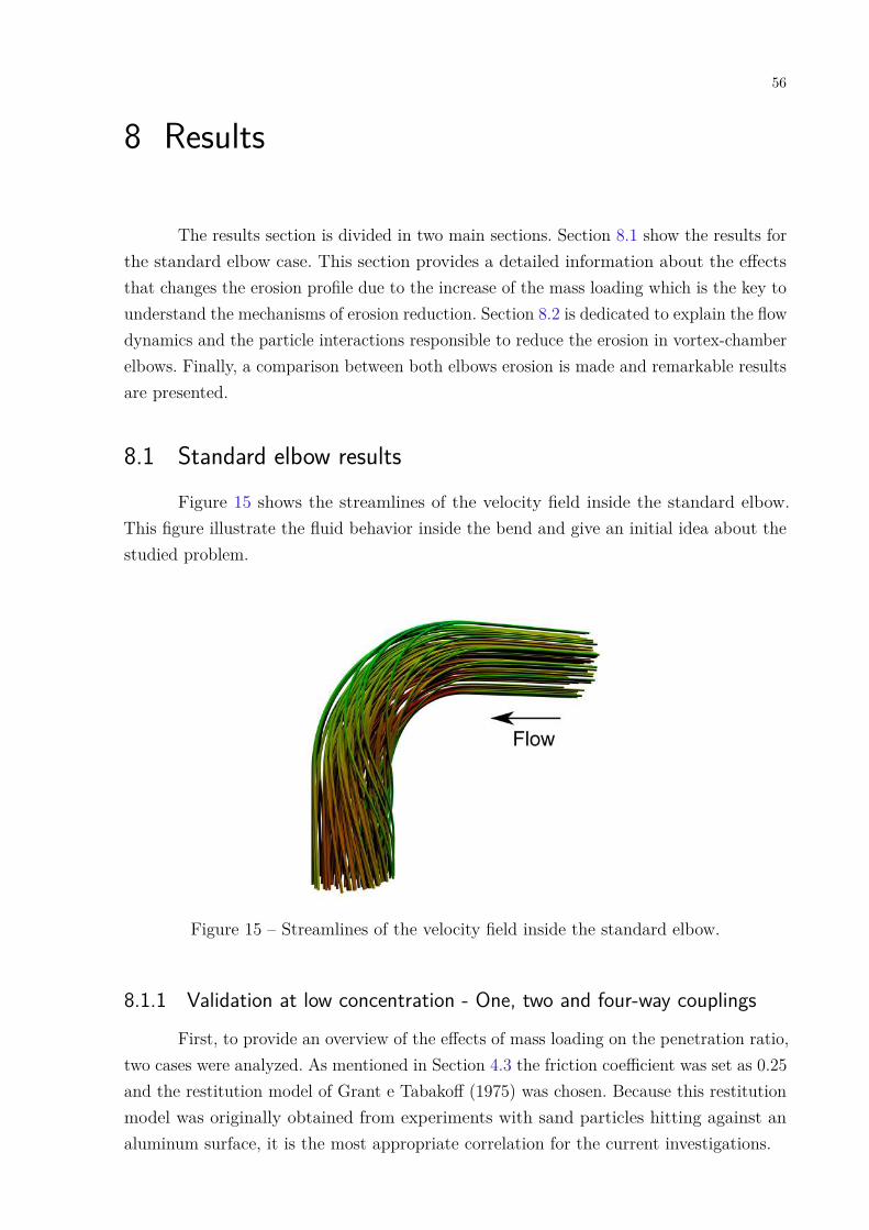
56
8 Results
The results section is divided in two main sections. Section 8.1 show the results forthe standard elbow case. This section provides a detailed information about the effectsthat changes the erosion profile due to the increase of the mass loading which is the key tounderstand the mechanisms of erosion reduction. Section 8.2 is dedicated to explain the flowdynamics and the particle interactions responsible to reduce the erosion in vortex-chamberelbows. Finally, a comparison between both elbows erosion is made and remarkable resultsare presented.
8.1 Standard elbow resultsFigure 15 shows the streamlines of the velocity field inside the standard elbow.
This figure illustrate the fluid behavior inside the bend and give an initial idea about thestudied problem.
Figure 15 – Streamlines of the velocity field inside the standard elbow.
8.1.1 Validation at low concentration - One, two and four-way couplings
First, to provide an overview of the effects of mass loading on the penetration ratio,two cases were analyzed. As mentioned in Section 4.3 the friction coefficient was set as 0.25and the restitution model of Grant e Tabakoff (1975) was chosen. Because this restitutionmodel was originally obtained from experiments with sand particles hitting against analuminum surface, it is the most appropriate correlation for the current investigations.

Chapter 8. Results 57
The first test conducted in this work aims at validating the numerical resultsusing the experiments carried out by Mazumder, Shirazi e McLaury (2008). The originalexperiment was performed at low mass loading (φ = 0.013), and the contours of thepenetration ratio for one, two and four-way couplings, seen from the opposite side of theinlet domain, are shown in Fig 16. It can be seen that, irrespective of the interactionregime, the contours of erosion are very similar, as well as the magnitude of the penetrationratio, quantitatively speaking. This general behavior was expected, since the mass loadingis low enough not to cause significant coupling between the two phases.
(a) (b) (c)
Figure 16 – Erosion contours of mass loading φ = 0.013 with different levels of interaction:(a) One-way coupling; (b) Two-way coupling; (c) Four-way coupling.
Based on the experimental data, it was also possible to quantitatively compare theerosion profile in the outer wall of the elbow as a function of the curvature angle. Theorigin (0) is set at the elbow inlet, and 90 corresponds to the elbow flow outlet (Fig. 11).Figure 17 shows the penetration ratio profile for one, two and four-way couplings, as wellas the experimental data by Mazumder, Shirazi e McLaury (2008) which also display therange of variation for each experimental point (each point was measured three times).
An analysis of Fig. 17 reveals that, independently of the interactions considered inthe simulation, for the mass loading of φ = 0.013, the model produces accurate resultswhen compared to the experiment. Up to this point, one-way coupling model wouldhave been sufficient to reproduce the experiment and to yield good results. Obviously,one-way coupling implies in much lower computational cost and a considerable reductionin simulation time. However, as will be demonstrated further, caution is necessary aboutthe choice of the coupling model. As the mass loading increases, neglecting interactionwith the fluid and inter-particle collisions may generate inaccurate results.
With the purpose of observing the effect of the coupling models in both phases, asecond test was conducted. The problem setup is identical to the previous one, but withthe mass loading set to φ = 0.25. Figure 18 illustrates the contours of penetration ratio

Chapter 8. Results 58
0 10 20 30 40 50 60 70 80 90
Curvature angle
0
1e-5
2e-5
3e-5
4e-5
5e-5
Penetr
ati
on r
ati
o (
m/k
g)
One-way coupling
Two-way coupling
Four-way coupling
Mazumder et al. 2008
Figure 17 – Numerical and experimental penetration ratios versus bend curvature anglefor one, two and four-way couplings. Mass loading φ = 0.013.
for the second test. Despite the relatively low mass loading (φ < 1), the penetration ratiocontours for the four-way calculation (Fig. 18c) is observed to be significantly differentfrom those obtained assuming only one-way (Fig. 18a), and two-way (Fig. 18b) couplings.The four-way coupling results show an extended region of maximum penetration and agradual softening around that location, whereas for one and two-way couplings, the shapeof the penetration ratio remains similar.
(a) (b) (c)
Figure 18 – Erosion contours of mass loading φ = 0.25 with different phase interactionregimes: (a) One-way coupling; (b) Two-way coupling; (c) Four-way coupling.
In this case, it is evident that the inter-particle collisions can directly influencethe erosion profile and cannot be ignored. This behavior can be seen in Fig. 19. It canbe observed from the erosion profile, that the two-way coupling results remain nearly

Chapter 8. Results 59
identical to the one-way coupling results. This means that the particles do not provide orextract enough momentum to alter the mean gas flow properties or its turbulence structure.Although the mass loading is greater than that of the first test, it is important to have inmind that these particles are rather inertial. Consequently, they not expected to be verysensitive to the continuous phase turbulence. Up to this point, it can be concluded thatthe collisions between particles are responsible for reducing the maximum penetrationratio magnitude in the elbow.
0 10 20 30 40 50 60 70 80 90
Curvature angle
0
1e-5
2e-5
3e-5
4e-5
5e-5
Penetr
ati
on r
ati
o (
m/k
g)
One-way coupling
Two-way coupling
Four-way coupling
Mazumder et al. 2008
Figure 19 – Numerical and experimental penetration ratio versus bend curvature anglefor one, two and four-way coupling and mass loading φ = 0.25.
The four-way calculation indicates how significant the inter-particle collisions canbe. The regions between 45 and 55, display a significant reduction of the penetrationratio peak (approximately 23 %). Another region, between 60 and 90, on the other hand,show that the penetration ratio is slightly increased.
Essentially, the results suggest that the inter particle collisions actually protectthe elbow surface from the direct impact from the incoming particles at the maximumpenetration location. Since the penetration ratio is cumulatively calculated, each individualcollision contributes to the erosion damage. Apparently, because of the inter-particlecollisions, the effective number of particles colliding with the wall in the maximumpenetration region is reduced, although an increase is visible downstream of such region.Because of the local high particle concentration, there is an increase of particle-to-particlecollision in the maximum impact region, which actually seems to shield the eroded surface.This phenomenon is outlined in Section 8.1.4.
An important conclusion of this first analysis is that the influence of inter-particlecollisions is important even at relatively moderate mass loadings, as demonstrated by

Chapter 8. Results 60
Souza, Silva e Utzig (2014) and Laín e Sommerfeld (2013).
In the next sections, the influence of the interaction of the particles with the carrierfluid and among themselves, the effects of the mass loading on the penetration ratio andthe mechanisms related to the cushioning effect will be analyzed.
8.1.2 Two-way versus four-way coupling
Before attempting to understand the effects of increasing mass loadings on theerosion, a comparison between results for two (lines with symbols) and four-way (dashedlines) for two different mass loadings is made in Fig. 20.
0 10 20 30 40 50 60 70 80 90
Curvature angle
0
1e-5
2e-5
3e-5
4e-5
5e-5
Penetr
ati
on r
ati
o (
m/k
g)
φ=0.25, four-way coupling
φ=0.25, two-way coupling
φ=1.0, four-way coupling
φ=1.0, two-way coupling
Mazumder et al. 2008
Figure 20 – Influence of two-way (lines with symbols) and four-way (dashed lines) couplingfor φ = 0.25 and φ = 1.0.
It can be concluded that in two-way coupling the penetration ratio is exactly thesame for the mass loadings of φ = 0.25 and φ = 1.0. This demonstrates that even at highermass loading, the particles do not significantly affect the gas flow enough to cause changesin the penetration ratio.
However, in the four-way coupling case, a characteristic reduction in penetrationratio is observed when the mass loading is increased. This finding corroborates the conclu-sions of the previous section: the particle-to-particle collisions play the most importantrole in attenuating the erosion peaks.
It has been shown in a number of papers (LAíN; SOMMERFELD, 2012) that theinter-particle collisions tend to make both particle and gas flows more homogeneous byflattening the velocity profiles in the pipe cross-section. Since the erosion rate is directlyproportional to a power of the impact velocity (cf. Eq. 4.48), a reduction in the penetration
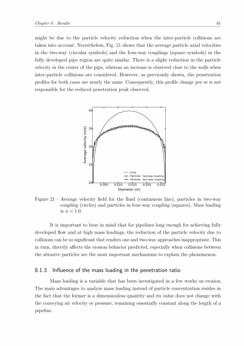
Chapter 8. Results 61
might be due to the particle velocity reduction when the inter-particle collisions aretaken into account. Nevertheless, Fig. 21 shows that the average particle axial velocitiesin the two-way (circular symbols) and the four-way couplings (square symbols) in thefully developed pipe region are quite similar. There is a slight reduction in the particlevelocity in the center of the pipe, whereas an increase is observed close to the walls wheninter-particle collisions are considered. However, as previously shown, the penetrationprofiles for both cases are nearly the same. Consequently, this profile change per se is notresponsible for the reduced penetration peak observed.
0.005 0.010 0.015 0.020 0.025
Diameter (m)
20
25
30
35
40
Avera
ge v
elo
city
(m
/s)
Fluid
Particles - two-way coupling
Particles - four-way coupling
Figure 21 – Average velocity field for the fluid (continuous line), particles in two-waycoupling (circles) and particles in four-way coupling (squares). Mass loadingis φ = 1.0.
It is important to bear in mind that for pipelines long enough for achieving fullydeveloped flow and at high mass loadings, the reduction of the particle velocity due tocollisions can be so significant that renders one and two-way approaches inappropriate. Thisin turn, directly affects the erosion behavior predicted, especially when collisions betweenthe abrasive particles are the most important mechanisms to explain the phenomenon.
8.1.3 Influence of the mass loading in the penetration ratio
Mass loading is a variable that has been investigated in a few works on erosion.The main advantages to analyze mass loading instead of particle concentration resides inthe fact that the former is a dimensionless quantity and its value does not change withthe conveying air velocity or pressure, remaining essentially constant along the length of apipeline.

Chapter 8. Results 62
In order to investigate the influence of the mass loading, five cases with φ equalto 0.013, 0.25, 0.5, 1.0 and 1.5 respectively, were then run to assess their effect in thepenetration ratio. Naturally, all cases considered particle-to-particle collisions. Figure 22displays the penetration ratio as a function of the curvature angle for the five cases studied.
0 10 20 30 40 50 60 70 80 90
Curvature angle
0
1e-5
2e-5
3e-5
4e-5
5e-5Penetr
ati
on r
ati
o (
m/k
g)
φ=0.013
φ=0.25
φ=0.5
φ=1.0
φ=1.5
Mazumder et al. 2008
Figure 22 – Influence of the mass loading in the penetration ratio.
The gradual reduction in the peak of the penetration ratio with the mass loadingincrease, known as cushioning effect, is clearly noticed. Visually speaking, the penetrationratio peak exponentially decays as the mass loading increases, which agrees with thefindings of Mills (2004). Somehow, this behavior contradicts the common sense, since itwas expected that the injection of a larger amount of erosive particles would result in ahigher penetration ratio.
The physical explanation for this reduction is entirely related to the inter-particlecollisions, as mentioned in previous sections. As the mass loading increases, more inter-particle collisions occur and less particle-to-wall collisions take place, especially in thepeak region of the penetration ratio. The layer of particles immediately adjacent tothe wall damps the impact of incoming particles to the elbow surface, reducing themagnitude of the penetration. This has been named "cushioning effect". This effect hasbeen observed experimentally (BIKBAEV et al., 1979), but has not been captured bysimulations, to the best of the author knowledge. The region between 0 and 45 of Fig.22 shows no modification with the increase of the mass loading, which suggests that theparticle-to-particle collisions do not significantly affect the particle velocity upstream ofthe bend.
Figure 23 shows snapshots of a pulse of particles before and during the first collisionwith the elbow in one (Figs. 23a, 23b, 23c), two (Figs. 23d, 23e, 23f) and four-way (Figs.
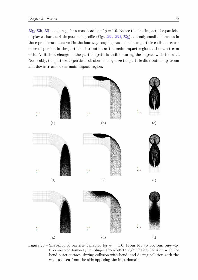
Chapter 8. Results 63
23g, 23h, 23i) couplings, for a mass loading of φ = 1.0. Before the first impact, the particlesdisplay a characteristic parabolic profile (Figs. 23a, 23d, 23g) and only small differences inthese profiles are observed in the four-way coupling case. The inter-particle collisions causemore dispersion in the particle distribution at the main impact region and downstreamof it. A distinct change in the particle path is visible during the impact with the wall.Noticeably, the particle-to-particle collisions homogenize the particle distribution upstreamand downstream of the main impact region.
(a) (b) (c)
(d) (e) (f)
(g) (h) (i)
Figure 23 – Snapshot of particle behavior for φ = 1.0. From top to bottom: one-way,two-way and four-way couplings. From left to right: before collision with thebend outer surface, during collision with bend, and during collision with thewall, as seen from the side opposing the inlet domain.

Chapter 8. Results 64
The penetration ratio contours for each mass loading of Fig. 22 are presented inFig. 24. It can be seen that the extension of maximum penetration is enlarged as themass loading increases. This a consequence of the more homogeneous particle distributionupstream of the elbow, as shown in Fig. 24.
(a) (b) (c)
(d) (e)
Figure 24 – Erosion contours with four-way coupling approach for the growing massloadings: (a) φ = 0.013; (b) φ = 0.25; (c) φ = 0.5; (d) φ = 1.0; (e) φ = 1.5.
Another distinctive feature is the modification of the inverted-V shape observed atthe lowest concentration. As the particle-to-particle collisions become more relevant, aline with increasing penetration becomes visible downstream of the elbow. A mechanicalexplanation for such phenomenon can be as complex as that for the rope formation inbends, and results directly from the enhanced inter-particle collisions.
The contours in Fig. 24 suggest that, after the first-colliding particles directlyimpact the elbow, they are reflected back to the core flow, resulting in particle interactionsthat prevent some of the incoming particles to reach the maximum erosion region. Instead,these incoming particles are deflect to different locations, especially downstream of theerosion peak. These interactions contribute significantly to change the erosion profile,reducing the maximum penetration ratio, but increasing it at new locations.
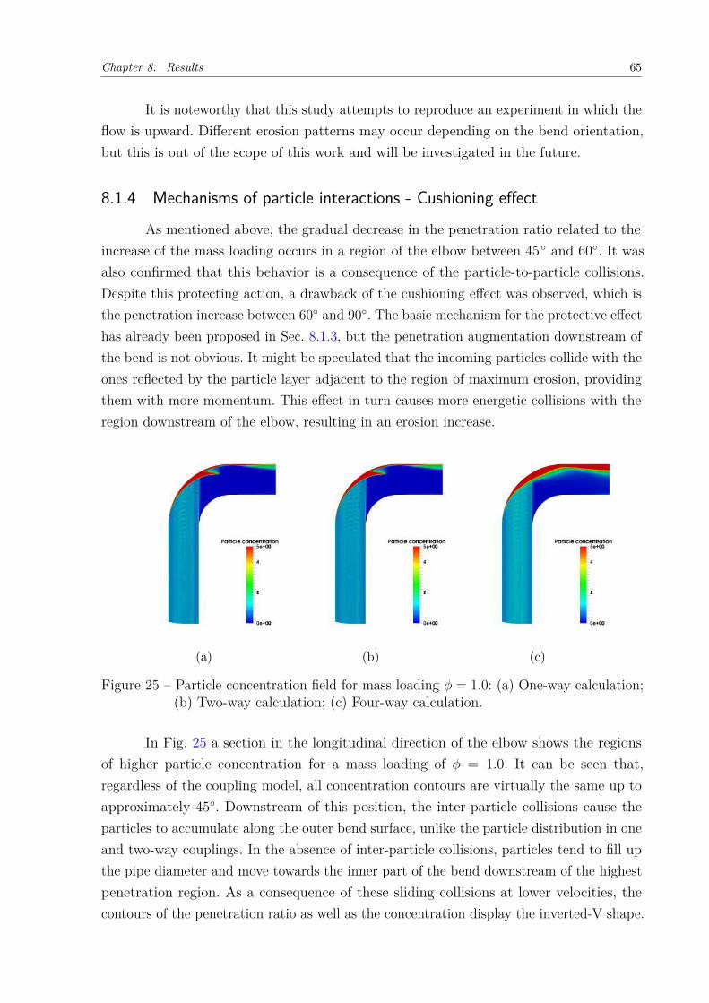
Chapter 8. Results 65
It is noteworthy that this study attempts to reproduce an experiment in which theflow is upward. Different erosion patterns may occur depending on the bend orientation,but this is out of the scope of this work and will be investigated in the future.
8.1.4 Mechanisms of particle interactions - Cushioning effect
As mentioned above, the gradual decrease in the penetration ratio related to theincrease of the mass loading occurs in a region of the elbow between 45 and 60. It wasalso confirmed that this behavior is a consequence of the particle-to-particle collisions.Despite this protecting action, a drawback of the cushioning effect was observed, which isthe penetration increase between 60 and 90. The basic mechanism for the protective effecthas already been proposed in Sec. 8.1.3, but the penetration augmentation downstream ofthe bend is not obvious. It might be speculated that the incoming particles collide with theones reflected by the particle layer adjacent to the region of maximum erosion, providingthem with more momentum. This effect in turn causes more energetic collisions with theregion downstream of the elbow, resulting in an erosion increase.
(a) (b) (c)
Figure 25 – Particle concentration field for mass loading φ = 1.0: (a) One-way calculation;(b) Two-way calculation; (c) Four-way calculation.
In Fig. 25 a section in the longitudinal direction of the elbow shows the regionsof higher particle concentration for a mass loading of φ = 1.0. It can be seen that,regardless of the coupling model, all concentration contours are virtually the same up toapproximately 45. Downstream of this position, the inter-particle collisions cause theparticles to accumulate along the outer bend surface, unlike the particle distribution in oneand two-way couplings. In the absence of inter-particle collisions, particles tend to fill upthe pipe diameter and move towards the inner part of the bend downstream of the highestpenetration region. As a consequence of these sliding collisions at lower velocities, thecontours of the penetration ratio as well as the concentration display the inverted-V shape.

Chapter 8. Results 66
In fact, for the one-way (Fig. 25a) and two-way (Fig. 25b) calculations, the concentrationprofile suffers a sharp discontinuity at a curvature angle close to 60.
When particle-to-particle collisions are included in the model, the above describedparticle motion is somehow inhibited. Instead of moving downwards along the pipe walls,the particles rebound from the main impact region actually collide with incoming particles.This effect, in turn, appears to push these particles back to the bend outer wall, whichexplains the high concentration downstream of the elbow along the pipe upper wall. Thisis also in accordance with the erosion patterns shown in Fig. 24 for higher mass loadings.Indeed, the particle-to-particle collisions are more elastic than the the particle-to-wallcollisions (the coefficient of restitution for the inter-particle collisions is 0.9).
8.2 Vortex-chamber elbow results
8.2.1 Fluid phase simulation
Before discussing about the particulate phase and its effects on erosion profile, thefluid field is presented. Figure 26 shows the streamlines of the velocity field in the regionof the vortex chamber. As expected, the flow does not suffer disturbances upstream of thechamber, while it is separated, on the wedge of the vortex chamber, downstream of theelbow. As a consequence, the well defined rotating vortex is generated inside the chamber.
Figure 26 – Streamlines of the velocity field inside the vortex-chamber elbow.
The contours of the velocity magnitude and turbulence kinetic energy are presentedin Fig. 27 for the symmetry plane. Within the first 30 degrees past the entrance of thevortex-chamber elbow, the flow adjusts to the transverse pressure gradient imposed bythe rotating flow inside the chamber and the location of the maximum velocity is shifted

Chapter 8. Results 67
toward the inner wall. About half-way through the elbow, the velocity contours show aregion of high velocity gradients near the inner wall. On the other hand, from the centerof the vortex chamber to about a diameter of the elbow entrance, the flow exhibits lowvelocity gradients. This region is called deflection zone and will be treated in details insection 8.2.2. As the flow exits and continues downstream in the pipe, it is no longeraffected by the transverse pressure gradient of the vortex chamber. This results in a shiftof the velocity maximum toward the outside wall.
(a) (b)
Figure 27 – Contours of velocity magnitude (a) and turbulence kinetic energy (b) insymmetry plane.
The contours of turbulence kinetic energy (TKE), presented in Fig. 27b, areconsistent with those of the velocity magnitude shown in Fig. 27a. As expected, the regionswith abrupt velocity gradients are associated with high values of velocity fluctuation thushigh values of turbulence kinetic energy.
8.2.2 Effects at low concentration - One, two and four-way coupling
Although there is no experimental data regarding the erosion process in vortex-chamber elbows, the validation for the standard elbow presented in Section 8.1.1 provedto be very accurate and will serve as a reference to predict the erosion effects on thevortex-chamber elbow. With this in mind, all the results discussed below will use the samemodels of erosion and restitution as well as its coefficients and material constants. Then, aplausible comparison between both elbows can be performed.
The first test conducted aimed to evaluate the effects on the erosion profile forboth φ = 0.013 and φ = 0.25 mass loadings. As stated before, φ = 0.013 represents theexperimental mass loading of the standard elbow (MAZUMDER; SHIRAZI; MCLAURY,2008). Figure 28 shows the erosion contours for the mass loading φ = 0.013 with one (Fig.28a), two (Fig. 28b) four-way (Fig. 28c) coupling. Qualitatively speaking, all coupling

Chapter 8. Results 68
approaches show similar characteristics, but the magnitude of penetration in the four-waycoupling is slightly lower than the others.
(a) (b) (c)
Figure 28 – Erosion contours of mass loading φ = 0.013 with different phase interactionregimes: (a) One-way coupling; (b) Two-way coupling; (c) Four-way coupling.
This reduction becomes evident when the erosion profile of the outer wall is observed(Fig. 29). For one and two-way coupling there are no significant variations in penetrationratio profile. This reveals that for two-way coupling, the continuous phase is not impactedby the discrete phase, and vice versa. When the collisions between particles are includedthe profile significantly reduces in all regions of the chamber. The peak of the penetrationratio occurs at 92.
0 10 20 30 40 50 60 70 80 90 100 110 120 130 140 150 160 170 180
Curvature angle
0
1e-5
2e-5
3e-5
4e-5
Penetr
ati
on r
ati
o (
m/k
g)
One-way coupling
Two-way coupling
Four-way coupling
Figure 29 – Numerical penetration ratio versus bend curvature angle for one, two andfour-way couplings. Mass loading φ = 0.013.
This preliminary result confirms what was expected, particles are rotating inside thevortex chamber and the collision between them is probably preventing incoming particlesto reach and increase the penetration ratio on the chamber wall. Despite the relatively low

Chapter 8. Results 69
mass loading employed, it is notable the importance of using four-way coupling approachfor this type of elbow. In this case, collisions between particles plays a decisive role inthe erosion reduction. Compared to the same mass loading of the standard elbow (Fig.17), a penetration peak reduction of 35.9% is observed. In the case of an initial test, thevortex-chamber elbow demonstrated a significant decrease in the penetration ratio andindicates that the results are promising.
In order to quantify the erosion effects due to the increase of the mass loading,a second test with φ = 0.25 was carried out and its contours for each type of couplingapproach are shown in Fig. 30.
(a) (b) (c)
Figure 30 – Erosion contours of mass loading φ = 0.25 with different phase interactionregimes: (a) One-way coupling; (b) Two-way coupling; (c) Four-way coupling.
For this case, no visible changes are seen in one (Fig. 30a) and two-way (Fig. 30b)coupling approaches, but the penetration ratio magnitude is slightly higher in the lastone. Surprisingly, in four-way (Fig. 30c) coupling, the contours change drastically. Theregion of maximum penetration ratio is notably expanded but its magnitude is greatlyreduced. This is the first indication of an effective relation between the increasing of themass loading and inter-particle collisions in the reduction of the penetration ratio.
To quantify the previous contours reduction, Fig. 31 shows the profiles for eachcoupling regime. Interestingly, as mentioned above, the peak penetration approach fortwo-way coupling has a slightly larger peak when compared to one-way. Although thedifference is very subtle in the region between 84 and 92, it can be stated that the fluidis adding momentum in the particles which contributes to increase their velocity andconsequently the penetration ratio. Despite being very inertial particles, after suffering thefirst collision to the chamber, the particles are forced by the prevailing velocity gradientsinside the chamber. This directly affects the exchange of momentum between both phasesand can not be captured with one-way coupling approach.
However, in the four-way coupling case, an impressive reduction in penetration ratio

Chapter 8. Results 70
is observed. By turning the particles collisions on, the peak reduction was 89.72% comparedto two-way coupling calculation. This effect proves that the inter-particle collisions are themost important mechanism in attenuating the penetration ratio in this type of elbow.
0 10 20 30 40 50 60 70 80 90 100 110 120 130 140 150 160 170 180
Curvature angle
0
1e-5
2e-5
3e-5
4e-5
Penetr
ati
on r
ati
o (
m/k
g)
One-way coupling
Two-way coupling
Four-way coupling
Figure 31 – Numerical penetration ratio versus bend curvature angle for one, two andfour-way couplings. Mass loading φ = 0.25.
Before showing the influence of different mass loadings in the penetration ratio,Section 8.2.3 gives an explanation of the effects observed when using only a two-waycoupling approach. This analysis provides us with valuable information on how the phasesexchange momentum between each other and how this influence the erosion profile.
8.2.3 Two-way coupling
The last result showed a small difference between one and two-way couplingcomputations. In order to quantify this difference for other mass loadings, five cases withφ equals to: 0.013, 0.25, 0.5, 1.0 and 1.5 were simulated and its contours are shown inFig. 32. Once again, no major modification in the penetration ratio is observed due to themass loading variation but its magnitude is slowly increasing as the mass loading becamehigher.
Figure 33 presents the penetration ratio profile for each mass loading above men-tioned. As the mass loading increases, notable increase in regions between 70 and 115
are seen. A similar behavior has been observed in direct numerical simulation by Bosse,Kleiser e Meiburg (2006). In two-way coupled simulations, the mechanism responsible forthe particle velocity enhancement can be explained by three contributing effects. The firstone is the inertia which forces particles to accumulate in regions of high strain and lowvorticity. The second effect, usually known as preferential sweeping, happens because thegravity is present. Its presence cause the particles to travel primarily toward regions of
Chapter 8. Results 71
downward fluid motion. Finally, the third effect is a local modification of the fluid velocitystructure by the particles in regions of increased particle concentration.
(a) (b) (c)
(d) (e)
Figure 32 – Erosion contours with two-way coupling approach for the growing mass load-ings: (a) φ = 0.013; (b) φ = 0.25; (c) φ = 0.5; (d) φ = 1.0; (e) φ = 1.5.
0 10 20 30 40 50 60 70 80 90 100 110 120 130 140 150 160 170 180
Curvature angle
0
1e-5
2e-5
3e-5
4e-5
5e-5
Penetr
ati
on r
ati
o (
m/k
g)
φ=0.013
φ=0.25
φ=0.5
φ=1.0
φ=1.5
Figure 33 – Numerical penetration ratio versus bend curvature angle with two-way couplingapproach for the growing mass loadings: (a) φ = 0.013; (b) φ = 0.25; (c)φ = 0.5; (d) φ = 1.0; (e) φ = 1.5.

Chapter 8. Results 72
As a result, the vertical configuration of the vortex-chamber elbow contributes toguide low mass loading particles to concentrate in low velocity regions (Fig. 27a) faster.As the mass loading increases, it takes longer time to particles reach this regions, forcingthem to hit more times in the outer chamber surface. This can explain why the increase ofthe mass loading is increasing the penetration ratio in two-way coupling.
Figures 34a and 34b shows the ”w” mean velocity component of the fluid andparticles, respectively. These values were taken from a line in the symmetry plane passingexactly in the center of the vortex chamber and perpendicular to the upward direction ofthe flow. The mean fluid velocity in this region presents an interesting behavior as themass loading is increased. The rotative profile is clearly observed for all the mass loadingbut is perfectly achieved for φ = 0.013. For this mass loading the peak of the velocities arenearly 20 m/s. As the mass loading increases the velocity profiles are attenuated by theloss of momentum due to the presence of more particles in the flow. As a consequence, themean particles velocity are enhanced (Fig. 34b) affecting the penetration ratio profile.
0.015 0.020 0.025 0.030 0.035 0.040 0.045 0.050
Chamber diameter (m)
-20
-15
-10
-5
0
5
10
15
20
Avera
ge v
elo
city
(m
/s)
φ=0.013
φ=0.25
φ=0.5
φ=1.0
φ=1.5
(a)
0.015 0.020 0.025 0.030 0.035 0.040 0.045 0.050
Chamber diameter (m)
-20
-15
-10
-5
0
5
10
15
20
Avera
ge v
elo
city
(m
/s)
φ=0.013
φ=0.25
φ=0.5
φ=1.0
φ=1.5
(b)
Figure 34 – Average velocity inside the vortex chamber: (a) fluid, (b) particle.
It is important to have in mind that this analyses involves a certain level ofcomplexity due to the nature of the flow and the 3 dimensional effects. The next Section isdedicated to show and explain the penetration ratio profiles when inter-particles collisionsare present.
8.2.4 Influence of the mass loading in the penetration ratio - Four-way coupling
In order to investigate the influence of the mass loading, five cases with thesame mass loading of the last section were simulated. The difference now is that all thecases considered particle-to-particle collisions. Figure 35 displays the penetration ratio

Chapter 8. Results 73
contours for the five cases studied. The erosion contours shows an extreme reduction ofthe penetration ratio magnitude from φ = 0.013 to φ = 1.5.
(a) (b) (c)
(d) (e)
Figure 35 – Erosion contours with four-way coupling approach for the growing massloadings: (a) φ = 0.013; (b) φ = 0.25; (c) φ = 0.5; (d) φ = 1.0; (e) φ = 1.5.
As expected, inter-particles collision is the most important effect related to thepenetration ratio reduction in vortex-chamber elbows. To better visualize the contoursof the penetration ratio for each mass loading and understand its impact for each case,the penetration ratio magnitude for φ = 1.5 was fixed and the others mass loading wereplotted based o its magnitude (Fig. 36).
For φ = 0.013 (Fig. 36a), practically all the surface of the vortex chamber hashigher penetration ratio values compared to φ = 1.5 (Fig. 36e). As the mass loading isincreased, the values that exceed the fixed one diminish but secondary regions presenterosion effects. The mass loading equals to: φ = 0.25 (Fig. 36b), φ = 0.5 (Fig. 36c), φ = 1.0(Fig. 36d) and φ = 1.5 (Fig. 36e) shows a new region of penetration ratio. This regionis present on the lateral part of the vortex chamber and can not be captured by oneand two-way coupling simulations. When four-way coupling is used, while some particlesrotates inside the chamber, incoming particles are forced to collide with them in orderto prevent direct impact to the vortex chamber wall. This collisions can result in twosituations. First, after the collision in the deflection zone the particles returns to main themain core flow and leave without hitting other surfaces. The second situation, which is

Chapter 8. Results 74
probably causing the lateral penetration ratio, is related to the redirection of the particlesto the lateral wall. After the collisions, instead of return to core flow, particles are directedto the nearest wall, resulting in the increase of the penetration ratio at this regions.
Although this lateral effect exists, its magnitude does not offer great concern abouta new failure location. The penetration ratio at this regions can be neglected compared tothe peak observed on the surface of the vortex chamber.
(a) (b) (c)
(d) (e)
Figure 36 – Erosion contours with four-way coupling approach for the growing massloadings: (a) φ = 0.013; (b) φ = 0.25; (c) φ = 0.5; (d) φ = 1.0; (e) φ = 1.5and fixed for φ = 1.5 magnitude.
Finally, the penetration ratio profile for each mass loading is quantitatively presentedin Figure 37. This result shows how effective the inter-particle collisions can be. Comparingφ = 0.013 to φ = 1.5 a peak reduction of 96.87 % is obtained. This impressive result showsthe capacity of the cushioning effect to reduce erosion wear.
As stated in Section 8.1.3, the abruptly reduction in the peak of the penetrationratio with the mass loading increase, caused by the cushioning effect, is clearly noticed.Once again, this behavior contradicts the common sense, but the vortex chamber structureprovides the perfect situation to take advantage of this mechanism.
The next section proposes the mechanisms responsible for the penetration ratioreduction and explains the cushioning effect. In addition, the deflection zone is presentedas well as its importance to the erosion reduction.
Chapter 8. Results 75
0 10 20 30 40 50 60 70 80 90 100 110 120 130 140 150 160 170 180
Curvature angle
0
5e-6
1e-5
1.5e-5
2e-5
2.5e-5
3e-5
Penetr
ati
on r
ati
o (
m/k
g)
φ=0.013
φ=0.25
φ=0.5
φ=1.0
φ=1.5
Figure 37 – Numerical penetration ratio versus bend curvature angle with four-way cou-pling approach for the growing mass loadings: (a) φ = 0.013; (b) φ = 0.25; (c)φ = 0.5; (d) φ = 1.0; (e) φ = 1.5.
8.2.5 Mechanisms of erosion reduction
As mentioned above, the abruptly decrease in the penetration ratio related to theincrease of the mass loading occurs in a preferred region of the vortex-chamber elbowbetween 10 and 120. In exception of φ = 0.013, the other mass loading simulations havea peculiar behavior between 125 and 175. It was also confirmed that this behavior is aconsequence of the particle-to-particle collisions and will be explained ahead.
Figure 38 shows a symmetry plane of the particle concentration for a mass loadingof φ = 1.5 in one (Fig. 38a), two (Fig. 38b) and four-way (Fig. 38c) coupling regimes.
(a) (b) (c)
Figure 38 – Particle concentration field for mass loading φ = 1.5: (a) One-way calculation;(b) Two-way calculation; (c) Four-way calculation.
It can be seen that one and two-way coupling model contours are quite similar.The major difference between them is the enlarged region in one-way approach of the
Chapter 8. Results 76
particle concentration just before the elbow entrance. In one-way coupling the particlesare totally driven by the carrier flow, this forces them to travel primarily to regions oflow velocity gradients (Fig. 27a) increasing the concentration at these locations (Fig. 38a).When particles feedback on fluid (two-way coupling), this concentration region attenuatesbut is still present. Even exchanging momentum with the fluid, the particles are carriedfor low-speed regions and remains there.
When particle-to-particle collisions are included in the model, the above describedconcentration region is displaced to the vicinity of the vortex chamber. Another visibledifference between four-way coupling and the others is the smoothed concentration contour.Two well-defined regions are responsible to the penetration reduction in four-way coupledsimulations. First, the convex region just before the vortex chamber, known as the deflectionzone. Second, the layer of particles near the surface of the vortex chamber. Before reachthe vortex chamber wall, the incoming particles are submitted to both regions and aredeflected or cushioned, respectively.
The cushioning effect here is much more effective when compared to the standardelbow but is important to highlight the deflection zone, which is not present in the standardelbow. This explain the rapidly reduction in the penetration observed before (Fig. 37) andgives us an idea of the benefits to combine this two mechanisms.
It is noteworthy that in one and two-way coupling a layer of particles exists nearthe vortex chamber wall but the absence of inter-particle collisions in the models do notallow a true assessment of the cushioning phenomenon.
8.2.6 Standard elbow versus Vortex-chamber elbow
Finally, Fig. 39 shows the penetration ratio profile of all the mass loadings studiedfor both elbow types. Such a comparison provides an overview of the complete analysesmade in this dissertation and help us understand the benefits of each elbow.
It is clearly seen that even the higher penetration ratio peak of the vortex-chamberelbow is smaller than the lower penetration ratio peak of the standard elbow. This resultshows the vortex-chamber elbow potential in reducing the penetration ratio. This efficiencyis enhanced as the mass loading is increased. An important conclusion resides in the flowregime, it is known that for high mass loading both elbows reduces the penetration ratio,but, as Fig. 39 reveals, the best situation for the vortex-chamber elbow occurs at highmass loadings. This findings is in accordance with HammerTek Corporation studies case,which affirms that the failure of the vortex-chamber takes at least 10 times longer thanthe standard elbow under the same operations circumstances.
This is the first time that a CFD tool captured this mechanisms of penetrationratio reduction and exposed the results to the research community. Even with some model

Chapter 8. Results 77
simplifications and using empirical correlations the results are remarkable.
0 10 20 30 40 50 60 70 80 90 100 110 120 130 140 150 160 170 180
Curvature angle
0
1e-5
2e-5
3e-5
4e-5
5e-5Penetr
ati
on r
ati
o (
m/k
g)
φ=0.013 - standard
φ=0.25 - standard
φ=0.5 - standard
φ=1.0 - standard
φ=1.5 - standard
φ=0.013 - vortex-chamber
φ=0.25 - vortex-chamber
φ=0.5 - vortex-chamber
φ=1.0 - vortex-chamber
φ=1.5 - vortex-chamber
Mazumder et al. 2008
Figure 39 – Comparison between the standard and the vortex-chamber elbows.
Table 3 provides a quantitative comparison of the peak of the penetration ratioreduction for both elbows, obviously, in four-way coupling. The percentage of reduction forφ = 1.5 illustrates the gain for adding a vortex chamber which is approximated 97%. Forindustrial purpose a reduction of this magnitude can save a lot of money on maintenance.The table also shows that even for smaller mass loadings the vortex chamber proves to bean attractive alternative to the standard elbow.
Table 3 – Standard elbow (SE) and vortex-chamber elbow (VCE) peak reduction.
Mass loading SE peak (m/kg) VCE peak (m/kg) Peak reduction (%)φ = 0.013 4.767E-5 3.052E-5 35.97φ = 0.25 3.765E-5 4.392E-6 88.33φ = 0.5 3.564E-5 3.182E-6 91.07φ = 1.0 3.365E-5 2.414E-6 92.82φ = 1.5 3.242E-5 9.522E-7 97.06
These results amongst the results of the rest of the research are concluded in totalin the next chapter.

78
9 Conclusions
The current study has focused on the behavior of erosion in both standard andvortex-chamber elbows. One validation erosion model supported in the creation of adecent simulation setup, after which the resulting setup was employed for simulating thevortex-chamber elbow. The current study has produced a simulation setup that is ableto predict erosion phenomena inside pipe fittings with sufficient accuracy. Moreover ithas revealed that including the vortex chamber geometry has a positive effect on thepenetration ratio reduction.
Below a more elaborate discussion is presented concerning the separate phases inthe research, i.e. the standard elbow and the cushioning effect in the validation phase andthe vortex-chamber elbow simulations in the analysis phase.
Validation phaseBy using accurate CFD models for the gas-particle flow within a ninety-degree-
elbow, it was possible to better understand the particle behavior and its consequences onthe erosion. A major feature of this validation has been the numerical investigation of themass loading effects on the erosion ratio.
Based on the simulation results, it can be concluded that even at low mass loadings,the effects of inter-particle collisions on the penetration ratio cannot be disregarded. Themain contribution of this work is the prediction and evaluation of the cushioning effectin elbow erosion. It is noteworthy that such effect has been noticed experimentally andcan be present in several industrial situations. It may also be the key to understandingerosion-related problems.
The decay of the penetration ratio with increasing the mass loading was foundto be due to particle-to-particle collisions. Although this phenomenon may appear asbeneficial, it is important to bear in mind that equipment regions not subject to erosionat low particle concentrations might become susceptible at higher concentrations.
Analysis phaseSince many industrial processes requires the transportation of high mass loading,
the vortex-chamber elbow appears as a very interesting alternative. Based on the simulationresults, it can be concluded that the vortex-chamber elbow show its full potential whendealing with dense phases despite showing efficient for low mass loadings as well.
Due to the excellent agreement of the numerical computations obtained with the

Chapter 9. Conclusions 79
validation phase in combination with all required models for the erosion prediction, it maybe concluded that the models presented here are capable for supporting the optimizationand the design of pneumatic conveying systems. In addition, with the knowledge of theinter-particles collision effects it will be now also possible to predict erosion rates in thedifferent pipe elements.
The deflecting and cushioning effects demonstrated to be the key in reducing vortex-chamber elbow erosion. With this in mind, this report contributes to the development ofnew geometries that can benefit from such effects.
Although the research objective is fulfilled, new interesting topics for future researchhave emerged. The subsequent chapter discusses those topics. Moreover, it provides severalillustrations for different simulations.

80
10 Future research
In the current research it was only possible to study the erosion process isolated.Although the outcome was satisfying, some topics may be interesting for future research.These topics are listed below:
• change the elbows configuration;
• change fluid and particles properties;
• analyze erosion in cyclone separators;
• consider unsteady simulations of the particle-laden flow using Large Eddy Simula-tions;
• add corrosion models to work alongside with erosion models.

81
Bibliography
AHLERT, K. Effects of Particle Impingement Angle and Surface Wetting on Solid ParticleErosion of AISI 1018 Steel. [S.l.]: University of Tulsa, 1994. Cited 3 times on pages 27,28, and 48.
ASKELAND, D.; FULAY, P.; WRIGHT, W. The Science and Engineering of Materials .[S.l.]: Cengage Learning, 2010. ISBN 9780495296027. Cited on page 22.
BENSON, M.; TANAKA, T.; EATON, J. K. Effects of Wall Roughness on ParticleVelocities in a Turbulent Channel Flow. Journal of Fluids Engineering, v. 127, n. 2, p.250–256, dez. 2004. ISSN 0098-2202. Cited on page 39.
BIKBAEV, F. A. et al. Main factors affecting gas abrasive wear of elbows in pneumaticconveying pipes. Chemical and Petroleum Engineering, v. 9, n. 1, p. 35–36, 1979. Citedon page 62.
BOSSE, T.; KLEISER, L.; MEIBURG, E. Small particles in homogeneous turbulence:Settling velocity enhancement by two-way coupling. Physics of Fluids (1994-present), v. 18,n. 2, p. –, 2006. Cited on page 70.
BOUSSINESQ, J. Essai sur la théorie des eaux courantes. [S.l.]: Imprimerie Nationale, 1877.(Mémoires présentés par divers savants à l’Académie des sciences de l’Institut national deFrance). Cited on page 34.
BREUER, M.; ALLETTO, M.; LANGFELDT, F. Sandgrain roughness model for roughwalls within eulerian–lagrangian predictions of turbulent flows. International Journal ofMultiphase Flow, v. 43, n. 0, p. 157 – 175, 2012. ISSN 0301-9322. Cited on page 38.
CHEN, X.; MCLAURY, B. S.; SHIRAZI, S. A. Application and experimental validationof a computational fluid dynamics (cfd)-based erosion prediction model in elbows andplugged tees. Computers & Fluids, v. 33, n. 10, p. 1251 – 1272, 2004. ISSN 0045-7930.Cited on page 27.
CHEN, X.; MCLAURY, B. S.; SHIRAZI, S. A. Numerical and experimental investigation ofthe relative erosion severity between plugged tees and elbows in dilute gas/solid two-phaseflow. Wear, v. 261, n. 7–8, p. 715 – 729, 2006. ISSN 0043-1648. Cited on page 27.
CROWE, C.; MICHAELIDES, E.; SCHWARZKOPF, J. Multiphase Flow Handbook.[S.l.]: Taylor & Francis, 2005. (Mechanical and Aerospace Engineering Series). ISBN9781420040470. Cited on page 38.
CROWE, C. et al. Multiphase Flows with Droplets and Particles. [S.l.]: Taylor & Francis,1997. ISBN 9780849394690. Cited on page 38.
DENNIS, S. C. R.; SINGH, S. N.; INGHAM, D. B. The steady flow due to a rotatingsphere at low and moderate reynolds numbers. Journal of Fluid Mechanics, v. 101, p.257–279, 11 1980. ISSN 1469-7645. Cited on page 37.

Bibliography 82
DESHPANDE, N.; BARIGOU, M. The flow of gas–liquid foams through pipe fittings.International Journal of Heat and Fluid Flow, v. 22, n. 1, p. 94 – 101, 2001. ISSN 0142-727X.Cited on page 25.
DUARTE, C. A. R.; SOUZA, F. J. de; dos Santos, V. F. Numerical investigation of massloading effects on elbow erosion. Submitted to Powder Technology - Ref. No.: ??, Elsevier,2015. Cited on page 40.
ELGHOBASHI, S. On predicting particle-laden turbulent flows. Applied Scientific Research,Kluwer Academic Publishers, v. 52, n. 4, p. 309–329, 1993. ISSN 0003-6994. Cited onpage 49.
FERZIGER, J. H.; PERIC, M. Computational methods for fluid dynamics. [S.l.]: Springer,2002. Cited 4 times on pages 43, 44, 46, and 47.
FINNIE, I. Erosion of surfaces by solid particles. Wear, v. 3, n. 2, p. 87 – 103, 1960. ISSN0043-1648. Cited 2 times on pages 22 and 23.
FORDER, A.; THEW, M.; HARRISON, D. A numerical investigation of solid particleerosion experienced within oilfield control valves. Wear, v. 216, n. 2, p. 184 – 193, 1998.ISSN 0043-1648. Cited 2 times on pages 30 and 48.
FRöHLICH, J.; TERZI, D. von. Hybrid les/rans methods for the simulation of turbulentflows. Progress in Aerospace Sciences, v. 44, n. 5, p. 349 – 377, 2008. ISSN 0376-0421.Cited 2 times on pages 9 and 32.
GAHR, K. Z. Microstructure and Wear of Materials. [S.l.]: Elsevier, 1987. v - vi p.(Tribology Series, v. 10). ISSN 0167-8922. Cited on page 22.
GRANT, G.; TABAKOFF, W. Erosion Prediction in Turbomachinery Resulting fromEnvironmental Solid Particles. Journal of Aircraft, American Institute of Aeronautics andAstronautics, v. 12, n. 5, p. 471–478, maio 1975. ISSN 0021-8669. Cited 5 times on pages30, 40, 41, 48, and 56.
GUIDE, F. Fluent 6.2 User Guide. Centerra Resource Park, 10 Cavendish Court, Lebanon,NH 03766, USA, 2005. Cited on page 43.
HASELBACHER, A.; NAJJAR, F.; FERRY, J. An efficient and robust particle-localizationalgorithm for unstructured grids. Journal of Computational Physics, v. 225, n. 2, p. 2198 –2213, 2007. ISSN 0021-9991. Cited 2 times on pages 39 and 51.
HUMPHREY, J. Fundamentals of fluid motion in erosion by solid particle impact. Inter-national Journal of Heat and Fluid Flow, v. 11, n. 3, p. 170 – 195, 1990. ISSN 0142-727X.Cited 2 times on pages 9 and 24.
HUTCHINGS, I. M. Tribology: friction and wear of engineering materials. [S.l.]: EdwardArnold, 1992. (Metallurgy and materials science). Cited 2 times on pages 22 and 23.
JONES, W.; LAUNDER, B. The prediction of laminarization with a two-equation modelof turbulence. International Journal of Heat and Mass Transfer, v. 15, n. 2, p. 301 – 314,1972. ISSN 0017-9310. Cited on page 34.

Bibliography 83
LAIN, S.; SOMMERFELD, M.; KUSSIN, J. Experimental studies and modelling of four-way coupling in particle-laden horizontal channel flow. International Journal of Heat andFluid Flow, v. 23, n. 5, p. 647 – 656, 2002. ISSN 0142-727X. Cited on page 39.
LAíN, S.; SOMMERFELD, M. Numerical calculation of pneumatic conveying in horizontalchannels and pipes: Detailed analysis of conveying behaviour. International Journal ofMultiphase Flow, v. 39, n. 0, p. 105 – 120, 2012. ISSN 0301-9322. Cited 2 times on pages49 and 60.
LAíN, S.; SOMMERFELD, M. Characterisation of pneumatic conveying systems usingthe euler/lagrange approach. Powder Technology, v. 235, n. 0, p. 764 – 782, 2013. ISSN0032-5910. Cited 5 times on pages 9, 27, 49, 50, and 60.
LAUNDER, B.; SHARMA, B. Application of the Energy-dissipation Model of Turbulenceto the Calculation of Flow Near a Spinning Disc. [S.l.]: Imperial College of Science andTechnology, Department of Mechanical Engineering, 1974. Cited on page 34.
LEVEQUE, R. J. Finite-volume methods for non-linear elasticity in heterogeneous media.International Journal for Numerical Methods in Fluids, John Wiley & Sons, Ltd., v. 40,n. 1-2, p. 93–104, 2002. ISSN 1097-0363. Cited on page 43.
LUN, C.; LIU, H. Numerical simulation of dilute turbulent gas-solid flows in horizontalchannels. International Journal of Multiphase Flow, v. 23, n. 3, p. 575 – 605, 1997. ISSN0301-9322. Cited on page 37.
MATHUR, S. R.; MURTHY, J. Y. A pressure-based method for unstructured meshes.Numerical Heat Transfer, Part B: Fundamentals, v. 31, n. 2, p. 195–215, 1997. Cited 2times on pages 43 and 45.
MAZUMDER, Q. H.; SHIRAZI, S. A.; MCLAURY, B. Experimental investigation ofthe location of maximum erosive wear damage in elbows. Journal of Pressure VesselTechnology, v. 130, n. 1, p. 1–7, 2008. ISSN 00949930. Cited 4 times on pages 27, 52, 57,and 67.
MEI, R. An approximate expression for the shear lift force on a spherical particle at finitereynolds number. International Journal of Multiphase Flow, v. 18, n. 1, p. 145 – 147, 1992.ISSN 0301-9322. Cited on page 37.
MILLS, D. Pneumatic conveying design guide. 2nd. ed. Burlington: Elsevier, 2004. ISBN 07506 5471 6. Cited 3 times on pages 17, 25, and 62.
NEILSON, J.; GILCHRIST, A. Erosion by a stream of solid particles. Wear, v. 11, n. 2, p.111 – 122, 1968. ISSN 0043-1648. Cited 3 times on pages 27, 28, and 48.
OESTERLE, B.; PETITJEAN, A. Simulation of particle-to-particle interactions in gassolid flows. International Journal of Multiphase Flow, v. 19, n. 1, p. 199 – 211, 1993. ISSN0301-9322. Cited on page 39.
OKA, Y.; OKAMURA, K.; YOSHIDA, T. Practical estimation of erosion damage causedby solid particle impact: Part 1: Effects of impact parameters on a predictive equation.Wear, v. 259, n. 1–6, p. 95 – 101, 2005. ISSN 0043-1648. 15th International Conference onWear of Materials. Cited on page 27.

Bibliography 84
OKA, Y.; OKAMURA, K.; YOSHIDA, T. Practical estimation of erosion damage causedby solid particle impact: Part 2: Mechanical properties of materials directly associatedwith erosion damage. Wear, v. 259, n. 1–6, p. 102 – 109, 2005. ISSN 0043-1648. 15thInternational Conference on Wear of Materials. Cited 4 times on pages 27, 40, 41, and 48.
PARISHER, R. A.; RHEA, R. A. Chapter 3 - pipe fittings. In: PARISHER, R. A.; RHEA,R. A. (Ed.). Pipe Drafting and Design (Second Edition). Second edition. Woburn: GulfProfessional Publishing, 2002. p. 13 – 47. ISBN 978-0-7506-7439-3. Cited on page 25.
PATANKAR, S. Numerical Heat Transfer and Fluid Flow . [S.l.]: Taylor & Francis, 1980.(Series in computational methods in mechanics and thermal sciences). ISBN 9780891165224.Cited on page 46.
PAULSON, J.; HESS, L. Short radius, low wear elbow. Google Patents, 1983. US Patent4,387,914. Disponível em: <http://www.google.com/patents/US4387914>. Cited on page26.
PENG, K. et al. An improved known vicinity algorithm based on geometry test for particlelocalization in arbitrary grid. Journal of Computational Physics , v. 228, n. 24, p. 9001 –9019, 2009. ISSN 0021-9991. Cited on page 50.
PEREIRA, G. C.; SOUZA, F. J.; MORO, D. A. Numerical prediction of the erosion dueto particles in elbows. Powder Technology, Elsevier, v. 261, p. 105–117, 2014. Cited 3times on pages 23, 24, and 40.
REYNOLDS, O. On the dynamical theory of incompressible viscous fluids and the deter-mination of the criterion. Philosophical Transactions of the Royal Society of London A:Mathematical, Physical and Engineering Sciences, The Royal Society, v. 186, p. 123–164,1895. ISSN 0264-3820. Cited on page 33.
ROTA, V. Vortice Ell Smart Elbow. Issue 1. RVB 89: [s.n.], 2001. Cited on page 26.
RUBINOW, S. I.; KELLER, J. B. The transverse force on a spinning sphere moving ina viscous fluid. Journal of Fluid Mechanics, v. 11, p. 447–459, 11 1961. ISSN 1469-7645.Cited on page 37.
SAFFMAN, P. G. The lift on a small sphere in a slow shear flow. Journal of FluidMechanics, v. 22, p. 385–400, 6 1965. ISSN 1469-7645. Cited on page 37.
SCHILLER, L.; NAUMANN, Z. A drag coefficient correlation. Ver. Deutsch. Ing., p.77–318, 1935. Cited on page 36.
SOMMERFELD, M. Validation of a stochastic lagrangian modelling approach for inter-particle collisions in homogeneous isotropic turbulence. International Journal of MultiphaseFlow, v. 27, n. 10, p. 1829 – 1858, 2001. ISSN 0301-9322. Cited 2 times on pages 36and 39.
SOMMERFELD, M.; HUBER, N. Experimental analysis and modelling of particle-wallcollisions. International Journal of Multiphase Flow, v. 25, n. 6–7, p. 1457 – 1489, 1999.ISSN 0301-9322. Cited 3 times on pages 30, 39, and 48.
SOUZA, F. J. de; SILVA, A.; UTZIG, J. Four-way coupled simulations of the gas-particleflow in a diffuser. Powder Technology, v. 253, p. 496–508, 2014. Cited on page 60.

Bibliography 85
TAKAHASHI, K. et al. Experimental study of low-cycle fatigue of pipe elbows with localwall thinning and life estimation using finite element analysis. International Journal ofPressure Vessels and Piping, v. 87, n. 5, p. 211 – 219, 2010. ISSN 0308-0161. Cited onpage 27.
TORO, E. Riemann Solvers and Numerical Methods for Fluid Dynamics: A PracticalIntroduction. [S.l.]: Springer, 2009. ISBN 9783540498346. Cited on page 43.
VERSTEEG, H.; MALALASEKERA, W. An Introduction to Computational Fluid Dy-namics: The Finite Volume Method. [S.l.]: Pearson Education Limited, 2007. ISBN9780131274983. Cited on page 43.
VIEIRA, R. E. et al. Experimental investigation of the effect of 90 degree standard elbowon horizontal gas–liquid stratified and annular flow characteristics using dual wire-meshsensors. Experimental Thermal and Fluid Science, v. 59, n. 0, p. 72 – 87, 2014. ISSN0894-1777. Cited 2 times on pages 26 and 27.
WILCOX, D. Turbulence Modeling for CFD. [S.l.]: DCW Industries, Incorporated, 1994.ISBN 9780963605108. Cited on page 34.
ZHANG, Y. et al. Comparison of computed and measured particle velocities and erosionin water and air flows. Wear, v. 263, n. 1–6, p. 330 – 338, 2007. ISSN 0043-1648. 16thInternational Conference on Wear of Materials. Cited 3 times on pages 27, 29, and 48.

Appendix

87
APPENDIX A – Additional illustrations
This appendix provide some illustrations that may be useful to better understandthe flow and the particles behavior inside both elbows. These illustrations are listed below.
1. Fig. 40, fluid velocity components of the standard elbow;
2. Fig. 41, pressure and turbulence kinetic energy of the standard elbow;
3. Fig. 42, fluid velocity components of the vortex-chamber elbow;
4. Fig. 43, pressure and turbulence kinetic energy of the vortex-chamber elbow;
5. Fig. 44, particles behavior inside the standard elbow (colored by diameter);
6. Fig. 45, particles behavior inside the standard elbow (colored by rotation);
7. Fig. 46, particles behavior inside the vortex-chamber elbow (colored by diameter);
8. Fig. 47, particles behavior inside the vortex-chamber elbow (colored by rotation).
9. Fig. 48, particles behavior for different coupling regimes (colored by velocity).

APPENDIX A. Additional illustrations 88
(a) (b)
(c)
Figure 40 – Standard elbow fields: (a) U velocity component; (b) V velocity component;(c) W velocity component.
(a) (b)
Figure 41 – Standard elbow fields: (a) Pressure; (b) Turbulence Kinetic Energy.

APPENDIX A. Additional illustrations 89
(a) (b)
(c)
Figure 42 – Vortex-chamber elbow fields: (a) U velocity component; (b) V velocity compo-nent; (c) W velocity component.
(a) (b)
Figure 43 – Vortex-chamber elbow fields: (a) Pressure; (b) Turbulence Kinetic Energy.

APPENDIX A. Additional illustrations 90
Figure 44 – Snapshot of particle behavior inside the standard elbow colored by diameter(one-way coupling).

APPENDIX A. Additional illustrations 91
Figure 45 – Snapshot of particle behavior inside the standard elbow colored by rotation:blue - low, red - high (one-way coupling).

APPENDIX A. Additional illustrations 92
Figure 46 – Snapshot of particle behavior inside the vortex-chamber elbow colored bydiameter (one-way coupling).

APPENDIX A. Additional illustrations 93
Figure 47 – Snapshot of particle behavior inside the vortex-chamber elbow colored byrotation: blue - low, red - high (one-way coupling).

APPENDIX A. Additional illustrations 94
(a) (b) (c)
(d) (e) (f)
(g) (h) (i)
Figure 48 – Snapshot of particles behavior for φ = 1.0. From top to bottom: 0.39s, 0.5sand 0.8s. From left to right: one-way, two-way and four-way coupling.


![CIP 2009.2010[1]](https://static.fdocumentos.tips/doc/165x107/577d37f61a28ab3a6b96c43f/cip-200920101.jpg)
