MODELOS DE ISING E POTTS ACOPLADOS AS …cpg/teses/Tese-JoseJavierCerdaHernandez.pdf · de ned in...
91
Transcript of MODELOS DE ISING E POTTS ACOPLADOS AS …cpg/teses/Tese-JoseJavierCerdaHernandez.pdf · de ned in...

MODELOS DE ISING E POTTS ACOPLADOS ASTRIANGULAÇÕES DE LORENTZ
José Javier Cerda Hernández
Dissertação/Tese apresentadaao
Instituto de Matemática e Estatísticada
Universidade de São Paulopara
obtenção do títulode
Doutor em Ciências
Programa: Estatística
Orientador: Prof. Dr. Anatoli Iambartsev
Coorientador: Prof. Dr. Yuri Suhov
Durante o desenvolvimento deste trabalho o autor recebeu auxílio nanceiro da
CAPES/FAPESP
São Paulo, junho de 2014

MODELOS DE ISING E POTTS ACOPLADOS ASTRIANGULAÇÕES DE LORENTZ
Esta é a versão original da dissertação/tese elaborada pelo
candidato José Javier Cerda Hernández, tal como
submetida à Comissão Julgadora.

Agradecimentos
First of all I would like to thank my supervisors Anatoli Iambartsev and Yuri Suhov for
guiding me through this research and their professional advisory and patience, as well as for
giving me the freedom to follow dierent themes during my research........
This work was supported by CAPES and FAPESP (projects 2012/04372-7 and 2013/06179-
2). Further, the author thanks the IME at the University of São Paulo for warm hospitality.
..........
i

ii

Resumo
José Javier Cerda Hernández. MODELOS DE ISING E POTTS ACOPLADOS
AS TRIANGULAÇÕES DE LORENTZ. 2010. 91 f. Tese (Doutorado) - Instituto de
Matemática e Estatística, Universidade de São Paulo, São Paulo, 2010.
O objetivo principal da presente tese é pesquisar : Quais são as propriedades do modelo de
Ising e Potts acoplado ao emsemble de CDT? Para estudar o modelo usamos dois metodos:
(1) Matriz de transferencia e Theorema de Krein-Rutman. (2) Representação FK para o
modelo de Potts sobre CDT e dual de CDT.
Matriz de transferencia permite obter propriedades espectrais da Matriz de transferencia
utilisando o Teorema de Krein-Rutman [KR48] sobre operadores que conservam o cone
de funções positivas. Também obtemos propriedades asintóticas da função de partição e
das medidas de Gibbs. Esses propriedades permitem obter uma região onde a energia livre
converge. O segundo método permite obter uma região onde a curva crítica do modelo
pode estar localizada. Alem disso, também obtemos uma limitante superior e inferior para
a energia livre a volume innito.
Finalmente, utilizando argumentos de dualidade em grafos e expansão em alta temper-
atura estudamos o modelo de Potts acoplado com triangulações causais. Essa abordagem
permite generalizar o modelo, melhorar os resultados obtidos para o modelo de Ising e obter
novas limitantes, superior e inferior, para a energia livre e para a curva crítica. Alem do
mais, obtemos uma aproximação do autovalor maximal do operador de transferencia a baixa
temperatura.
Palavras-chave: dinâmica de triangulações causais, modelo de Ising, modelo de Potts,
medida de Gibbs, Teorema de Krein-Rutman, representação FK, modelo de Ising quântico.
iii

iv
Abstract
José Javier Cerda Hernández. Ising and Potts model coupled to Lorentzian triangu-
lations. 2014. 91 f. Tese (Doutorado) - Instituto de Matemática e Estatística, Universidade
de São Paulo, São Paulo, 2014.
The main objective of the present thesis is to investigate: What are the properties of
the Ising and Potts model coupled to a CDT emsemble? For that objetive, we used two
methods: (1) transfer matrix formalism and Krein-Rutman theory. (2) FK representation of
the q-state Potts model on CDTs and dual CDTs.
Transfer matrix formalism permite us obtain spectral properties of the transfer matrix
using the Krein-Rutman theorem [KR48] on operators preserving the cone of positive func-
tions. This yields results on convergence and asymptotic properties of the partition function
and the Gibbs measure and allows us to determine regions in the parameter quarter-plane
where the free energy converges. Second methods permite us determining a region in the
quadrant of parameters β, µ > 0 where the critical curve for the classical model can be
located. We also provide lower and upper bounds for the innite-volume free energy.
FInally, using arguments of duality on graph theory and hight-T expansion we study
the Potts model coupled to CDTs. This approach permite us improve the results obtained
for Ising model and obtain lower and upper bounds for the critical curve and free energy.
Moreover, we obtain an approximation of the maximal eigenvalue of the transfer matrix at
lower temperature.
Keywords: causal dynamical triangulation, Ising model, Potts model, Gibbs measure,
Krein-Rutman theory, FK representation, quantum Ising model.
v

vi
Contents
List of Figures ix
1 Introduction 1
1.1 Introduction and statement results . . . . . . . . . . . . . . . . . . . . . . . 1
2 Two-dimensional causal dynamical Triangulations 5
2.1 Denitions . . . . . . . . . . . . . . . . . . . . . . . . . . . . . . . . . . . . . 5
2.2 Transfer matrix formalism for pure CDTs . . . . . . . . . . . . . . . . . . . . 7
3 Transfer matrix formalism for Ising model coupled to two-dimensional
CDT 13
3.1 The model . . . . . . . . . . . . . . . . . . . . . . . . . . . . . . . . . . . . . 13
3.2 The transfer-matrix K and its powers KN . . . . . . . . . . . . . . . . . . . 17
3.3 Discussion and outlook . . . . . . . . . . . . . . . . . . . . . . . . . . . . . . 25
4 FK representation for the Ising model coupled to CDT 27
4.1 The quantum Ising model . . . . . . . . . . . . . . . . . . . . . . . . . . . . 27
4.2 FK representation for Ising model coupled to CDT . . . . . . . . . . . . . . 29
4.3 The main results . . . . . . . . . . . . . . . . . . . . . . . . . . . . . . . . . 32
4.4 Proof of Theorem 4.3.1 and 4.3.2 . . . . . . . . . . . . . . . . . . . . . . . . 36
4.4.1 Proof of Theorem 4.3.1 . . . . . . . . . . . . . . . . . . . . . . . . . . 36
4.4.2 Proof of Theorem 4.3.2 . . . . . . . . . . . . . . . . . . . . . . . . . . 40
5 Potts model coupled to CDTs and FK representation 41
5.1 Introduction and main results of this chapter . . . . . . . . . . . . . . . . . . 41
5.2 Notations . . . . . . . . . . . . . . . . . . . . . . . . . . . . . . . . . . . . . 45
5.2.1 A Potts model coupled to CDTs . . . . . . . . . . . . . . . . . . . . . 45
5.2.2 The FK-Potts model on Lorentzian triangulations . . . . . . . . . . . 46
5.2.3 The relation between the Potts model and FK-Potts model: Edwards-
Sokal coupling . . . . . . . . . . . . . . . . . . . . . . . . . . . . . . . 47
5.2.4 Duality for FK-Potts model coupled to CDTs with periodic boundary
conditions . . . . . . . . . . . . . . . . . . . . . . . . . . . . . . . . . 48
5.3 The proof of Theorem 5.1.1 and rst bounds for the critical curve . . . . . . 52
vii

viii CONTENTS
5.4 High-T expansion of the Potts model and Proof of Theorem 5.1.2 . . . . . . 58
5.5 Connection between transfer matrix and FK representation . . . . . . . . . . 62
5.5.1 q = 2 (Ising) systems . . . . . . . . . . . . . . . . . . . . . . . . . . . 62
5.5.2 q-Potts systems . . . . . . . . . . . . . . . . . . . . . . . . . . . . . . 63
5.6 Discussion and outlook . . . . . . . . . . . . . . . . . . . . . . . . . . . . . . 68
A The von Neumann-Schatten Classes of Operators 71
A.1 The space Cp and rst properties . . . . . . . . . . . . . . . . . . . . . . . . 71
A.2 The trace class C1 . . . . . . . . . . . . . . . . . . . . . . . . . . . . . . . . . 72
A.3 The Banach space Cp . . . . . . . . . . . . . . . . . . . . . . . . . . . . . . . 72
A.4 The Hilbert-Schmidt class . . . . . . . . . . . . . . . . . . . . . . . . . . . . 74
B Krein-Rutman theorem 75
B.1 Krein-Rutman Theorem and the Principal Eigenvalue . . . . . . . . . . . . . 75
Bibliography 77
List of Figures
1.1 A strip of a causal triangulation of S × [j, j + 1]. . . . . . . . . . . . . . . . 2
2.1 (a) A strip of a causal triangulation of S × [j, j + 1]. (b) Geometric represen-
tation of a CDT with periodic spatial boundary condition. . . . . . . . . . . 7
2.2 Tree parametrization of a causal dynamical triangulation. . . . . . . . . . . . 11
3.1 Illustration of the calculates (3.25) and (3.27). . . . . . . . . . . . . . . . . . 22
3.2 λQ = λ and λT are the maximal eigenvalues of the matrix Q and a related
matrix T respectively. The area above the black curve is where the condition
(3.20) holds true. . . . . . . . . . . . . . . . . . . . . . . . . . . . . . . . . . 26
4.1 A trajectory sample associated with a realization ξ = sii=1,...,n. Each tra-
jectory ϕ ∈ ψξ can be continuous or not at each arrival time s. In this case,
at arrival time sk−1 the trajectory ϕ do not have jump, and at arrival time
sk the trajectory ϕ have a jump. . . . . . . . . . . . . . . . . . . . . . . . . 30
4.2 In this gure, we show the Cluster Ct of a triangle t, and a graphic represen-
tation of relation t↔ t′, where↔ on right side in the gure, represent arrival
times. . . . . . . . . . . . . . . . . . . . . . . . . . . . . . . . . . . . . . . . 31
4.3 The area above the minimum of the dotted curve I (graph of the function ψ
dened in (4.21)) and dash-dotted line II is where the limiting Gibbs proba-
bility measure exists and is unique. The critical curve lies in the region below
the dotted curve I and dash-dotted line II but above the continuous curve III
and dashed line IV. . . . . . . . . . . . . . . . . . . . . . . . . . . . . . . . . 35
5.1 Illustrating the region where the critical curve for Potts model coupled CDTs
and dual CDTs can be located. . . . . . . . . . . . . . . . . . . . . . . . . . 43
5.2 Geometric representation of a dual Lorentzian triangulation t∗ with periodic
spatial boundary condition. . . . . . . . . . . . . . . . . . . . . . . . . . . . 47
5.3 (a) Geometric representation of a net (b) Geometric representation of a cycle
(c) None of cluster of w is a net or a cycle . . . . . . . . . . . . . . . . . . . 49
5.4 Examples of three subgraphs of A with 8 edges. It is clear that the term
ξ(e1, . . . , e8) depends of the topology of the subgraphs. . . . . . . . . . . . . 59
ix

x LIST OF FIGURES
5.5 Region where the critical curve of the Ising model coupled to dual CDTs can
be located. . . . . . . . . . . . . . . . . . . . . . . . . . . . . . . . . . . . . . 63
5.6 The blue line is the simulation of ||A||2 = 1 for q = 4. Black line: µ∗ = 3 ln 2.
Green line: µ∗ = 32
ln(eβ∗ − 1
)+ ln 2. Red line: µ∗ = 3
2ln(42/3 + eβ
∗ − 1)
+ ln 2. 68
Chapter 1
Introduction
1.1 Introduction and statement results
Models of planar random geometry appear in physics in the context of two-dimensional
quantum gravity and provide an interplay between mathematical physics and probability
theory.
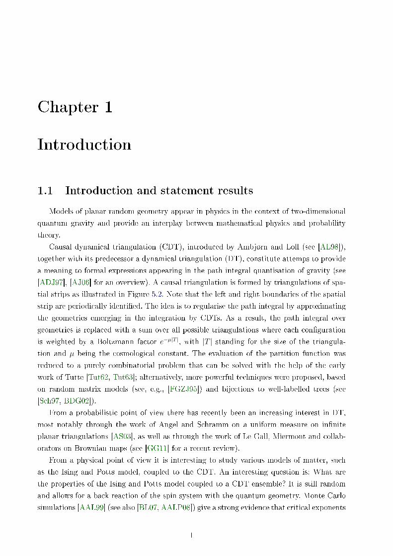
Causal dynamical triangulation (CDT), introduced by Ambjørn and Loll (see [AL98]),
together with its predecessor a dynamical triangulation (DT), constitute attemps to provide
a meaning to formal expressions appearing in the path integral quantisation of gravity (see
[ADJ97], [AJ06] for an overview). A causal triangulation is formed by triangulations of spa-
tial strips as illustrated in Figure 5.2. Note that the left and right boundaries of the spatial
strip are periodically identied. The idea is to regularise the path integral by approximating
the geometries emerging in the integration by CDTs. As a result, the path integral over
geometries is replaced with a sum over all possible triangulations where each conguration
is weighted by a Boltzmann factor e−µ|T |, with |T | standing for the size of the triangula-
tion and µ being the cosmological constant. The evaluation of the partition function was
reduced to a purely combinatorial problem that can be solved with the help of the early
work of Tutte [Tut62, Tut63]; alternatively, more powerful techniques were proposed, based
on random matrix models (see, e.g., [FGZJ95]) and bijections to well-labelled trees (see
[Sch97, BDG02]).
From a probabilistic point of view there has recently been an increasing interest in DT,
most notably through the work of Angel and Schramm on a uniform measure on innite
planar triangulations [AS03], as well as through the work of Le Gall, Miermont and collab-
orators on Brownian maps (see [GG11] for a recent review).
From a physical point of view it is interesting to study various models of matter, such
as the Ising and Potts model, coupled to the CDT. An interesting question is: What are
the properties of the Ising and Potts model coupled to a CDT ensemble? It is still random
and allows for a back-reaction of the spin system with the quantum geometry. Monte Carlo
simulations [AAL99] (see also [BL07, AALP08]) give a strong evidence that critical exponents
1

2 INTRODUCTION 1.1
root"up"
down"
S ×[ j, j +1]
Figure 1.1: A strip of a causal triangulation of S × [j, j + 1].
of the Ising model coupled to CDT are identical to the Onsager values. The calculation of the
partition function in this case also reduces to a combinatorial problem. It was rst solved in
[Kaz86, BK87] by using random matrix models and later by using a bijection to well-labelled
trees [BMS11]. It is interesting that the solution here is much simpler than in the case of
a at triangular or square lattice as given by Onsager [Ons44]. For the 2-state Potts model
(Ising model) coupled to CDTS some progress has been recently made on existence of Gibbs
measures and phase transitions (see [AAL99], [BL07], [HYSZ13] and [Her14] for details).
Using transfer matrix methods, the Krein-Rutman theory of positivity-preserving operators
and FK representation for the Ising model, [Her14] provides a region in the quadrant of
parameters β, µ > 0 where the innite-volume free energy has a limit, providing results on
convergence and asymptotic properties of the partition function and the Gibbs measure.
Thus, FK-Potts models, introduced by Fortuin and Kasteleyn (see [FK72]), prove that these
models have become an important tool in the study of phase transition for the Ising and
q-state Potts model.
The goal of this thesis is to use Krein-Rutman theory of positivity-preserving operators,
FK representation of the q-state Potts model on a xed triangulation and duality theory of
graph for study the q-state Potts model coupled to CDTs.
While recently much progress has been made in the development of analytical techniques
for CDT [JAZ07, JAZ08d], particularly random matrix models [JAZ08b, JAZ08a, JAZ08c],
and their application to multi-critical CDT [AGGS12, AZ12a, AZ12b], the causality con-
straints still makes it dicult to nd an analytical solution of the Ising model coupled to
CDT.
In this thesis we focus on study the q-state Potts model coupled to CDTs and is organised
as follows.
In Chapter 2 gives a summary of causal dynamical triangulations CDTs and we intro-

1.1 INTRODUCTION AND STATEMENT RESULTS 3
duced the transfer matrix formalism for pure CDTs. Also, we study asymptotic properties
of the partition function for pure CDTs. These properties will be used in next chapters.
In Chapter 3 we dene the annealed Ising model coupled to two-dimensional CDT and
develop a transfer matrix formalism. Spectral properties of the transfer matrix are rigorously
analysed by using the Krein-Rutman theorem [KR48] on operators preserving the cone
of positive functions. This yields results on convergence and asymptotic properties of the
partition function and the Gibbs measure and allows us to determine regions in the parameter
quarter-plane where the partition function converges. The main results of this chapter are
Lemma 3.2.1 and Theorem 3.2.2.
In Chapter 4 we use the Fortuin-Kasteleyn (FK) representation of quantum Ising models
via path integrals for determining a region in the quadrant of parameters β, µ > 0 where
the critical curve for the classical model can be located. In Section 4.1 we describe the
quantum Ising model. In Section 4.2, we give the FK representation of Ising model coupled
to CDTs via a path integral. This representation was originally derived in [MAC92] (see also
[Aiz94] and [Iof09]). Section 4.3 we present the main results of this chapter (Theorems 4.3.1
and 4.3.2). Section 4.4.1 and 4.4.2 contains the proof of Theorems 4.3.1 and 4.3.2. We also
provide lower and upper bounds for the innite-volume free energy. This chapter extends
results from Chapter 3 for the (annealed) Ising model coupled to two-dimensional causal
dynamical triangulations.
In Chapter 5. In Section 5.2, we introduce notation, dened the Potts model coupled
to CDTs and give a summary of the FK model, FK representation. Finally, we establish a
technical proposition of duality that will used in the next section. Section 5.3 contains the
proof of the rts main Theorem 5.1.1, and we nd a rst bounds for the critical curve. This
result will play a key role proof of the second main Theorem 5.1.2 of this chapter. In Section
5.4, using the High-T expansion for q-state Potts model, we prove Theorem 5.1.2.
Finally, Appendix A and B provide a review of trace class operators and Krein-Rutman
theory, used in Chapters 2 and 3.
Most of the novel results of this thesis have been published in research articles. In par-
ticular, the following chapters are based on the following articles:
• Chapter 2 and 3 on J.C. Hernández, Y. Suhov, A. Yambartsev, and S. Zohren, Bounds
on the critical line via transfer matrix methods for an Ising model coupled to causal
dynamical triangulations. J. Math. Phys. 54 063301 (2013).
• Chapter 4 on submitted paper, J. Cerda-Hernández, Critical region for an Ising model
coupled to causal dynamical triangulations. arxiv 1402.3251 (2014).
• Chapter 5 on preparation article, J. Cerda-Hernández, Duality relation for Potts model
coupled to causal dynamical triangulations (2014).

4 INTRODUCTION 1.1

Chapter 2
Two-dimensional causal dynamical
Triangulations
In this chapter we introduce causal dynamical triangulations (CDTs) as a discretization
of the partition function for two-dimensional quantum gravity. After giving a mathematical
denition of CDT we show some asymptotical properties of the partition function using
transfer matrix approach. These asymptotical properties will used in next sections.
2.1 Denitions
We will work with rooted causal dynamic triangulations of the cylinder CN = S × [0, N ],
N = 1, 2, . . . , which have N bonds (strips) S × [j, j+ 1]. Here S stands for a unit circle. The
denition of a causal triangulation starts by considering a connected graph G embedded
in CN with the property that all faces of G are triangles (using the convention that an
edge incident to the same face on two sides counts twice, see [SYZ13] for more details). A
triangulation t of CN is a pair formed by a graph G with the above propetry and the set F
of all its (triangular) faces: t = (G,F ).
Denition 2.1.1. A triangulation t of CN is called a causal triangulation (CT) if the
following conditions hold:
• each triangular face of t belongs to some strip S × [j, j + 1], j = 1, . . . , N − 1, and has
all vertices and exactly one edge on the boundary (S ×j)∪ (S ×j+ 1) of the stripS × [j, j + 1];
• if kj = kj(t) is the number of edges on S × j, then we have 0 < kj < ∞ for all
j = 0, 1, . . . , N − 1.
Denition 2.1.2. A triangulation t of CN is called rooted if it has a root. The root in the
triangulation t is represented by a triangular face t of t, called the root triangle, with an
anticlock-wise ordering on its vertices (x, y, z) where x and y belong to S1×0. The vertexx is identied as the root vertex and the (directed) edge from x to y as the root edge.
5

6 TWO-DIMENSIONAL CAUSAL DYNAMICAL TRIANGULATIONS 2.1
Denition 2.1.3. Two causal rooted triangulations of CN , say t = (G,F ) and t′ = (G′, F ′),
are equivalent if there exists a self-homeomorphism of CN which (i) transforms each slice
S1 × j, j = 0, . . . , N − 1 to itself and preserves its direction, (ii) induces an isomorphism
of the graphs G and G′ and a bijection between F and F ′, and (iii) takes the root of t to the
root of t′.
Let LTN and LT∞ denote the sets of causal triangulations on the nite cylinder CN and
innity cylinder C = S × [0,∞).
A triangulation t of CN is identied as a consistent sequence:
t = (t(0), t(1), . . . , t(N − 1)),
where t(i) is a causal triangulation of the strip S × [i, i + 1]. The latter means that each
t(i) is described by a partition of S × [i, i + 1] into triangles where each triangle has one
vertex on one of the slices S ×i, S ×i+ 1 and two on the other, together with the edge
joining these two vertices. The property of consistency means that each pair (t(i), t(i+ 1))
is consistent, i.e., every side of a triangle from t(i) lying in S × i+ 1 serves as a side of a
triangle from t(i+ 1), and vice versa.
The triangles forming the causal triangulation t(i) are denoted by t(i, j), 1 ≤ j ≤ n(t(i))
where, n(t(i)) stands for the number of triangles in the triangulation t(i). The enumeration
of these triangles starts with what we call the root triangle in t(i); it is determined recursively
as follows (see Figure 2.1(b)): First, we have the root triangle t(0, 1) in t(0) (see Denition
2.1.2). Take the vertex of the triangle t(0, 1) which lies on the slice S × 1 and denote it
by x′. This vertex is declared the root vertex for t(1). Next, the root edge for t(1) is the one
incident to x′ and lying on S×1, so that if y′ is its other end and z′ is the third vertex of the
corresponding triangle then x′, y′, z′ lists the three vertices anticlock-wise. Accordingly, the
triangle with the vertices x′, y′, z′ is called the root triangle for t(1). This construction can be
iterated, determining the root vertices, root edges and root triangles for t(i), 0 ≤ i ≤ N − 1.
It is convenient to introduce the notion of up" and down" triangles (see Figure 2.1(a)).
We call a triangle t ∈ t(i) an up-triangle if it has an edge on the slice S × i and a down-
triangle if it has an edge on the slice S×i+1. By Denition 2.1.1, every triangle is either of
type up or down. Let nup(t(i)) and ndo(t(i)) stand for the number of up- and down-triangles
in the triangulation t(i).
Note that for any edge lying on the slice S×i belongs to exactly two triangles: one up-
triangle from t(i) and one down-triangle from t(i− 1). This provides the following relation:
the number of triangles in the triangulation t is twice the total number of edges on the slices.
More precisely, let ni be the number of edges on slice S×i. Then, for any i = 0, 1, . . . , N−1,
n(t(i)) = nup(t(i)) + ndo(t(i)) = ni + ni+1, (2.1)

2.2 TRANSFER MATRIX FORMALISM FOR PURE CDTS 7
downtriangle up
triangle
S1×[ i, i +1]
root
(a) (b)
Figure 2.1: (a) A strip of a causal triangulation of S × [j, j + 1]. (b) Geometric representation of
a CDT with periodic spatial boundary condition.
implying thatN−1∑i=0
n(t(i)) = 2N−1∑i=0
ni. (2.2)
There is another useful property regarding the counting of triangulations. Let us x the
number of edges ni and ni+1 in the slices S × i and S × i + 1. The number of possible
rooted CTs of the slice S × [i, i+ 1] with ni up- and ni+1 down-triangles is equal to(ni + ni+1 − 1
ni − 1
)=
(n(t(i))− 1
nup(t(i))− 1
). (2.3)
2.2 Transfer matrix formalism for pure CDTs
We begin by discussing the case of pure causal dynamical triangulations, as was rst
introduced in [AL98] (see also [MYZ01] for a mathematically more rigorous account).
The partition function for rooted CTs in the cylinder CN with periodical spatial boundary
conditions (where t(0) is consistent with t(N − 1)) and for the value of the cosmological
constant µ is given by
ZN(µ) =∑t
e−µn(t) =∑
(t(0),...,t(N−1))
exp−µ
N−1∑i=0
n(t(i)). (2.4)
Using the properties (2.2) and (2.3) we can represent the partition function (2.4) in the
following way
ZN(µ) =∑
n0≥1,...,nN−1≥1
exp−2µ
N−1∑i=0
niN−1∏
i=0
(ni + ni+1 − 1
ni − 1
). (2.5)

8 TWO-DIMENSIONAL CAUSAL DYNAMICAL TRIANGULATIONS 2.2
Moreover, ZN(µ) admits a trace-related representation
ZN(µ) = tr(UN). (2.6)
This gives rise to a transfer matrix U = u(n, n′)n,n′=1,2,... describing the transition from
one spatial strip to the next one. It is an innite matrix with strictly positive entries
u(n, n′) =
(n+ n′ − 1
n− 1
)gn+n′ . (2.7)
For notational convenience we use the parameter g = e−µ (a single-triangle fugacity). The
entry u(n, n′) yields the number of possible triangluations of a single strip (say, S × [0, 1])
with n lower boundary edges (on S × 0) and n′ upper boundary edges (on S × 1). SeeFigure 5.2. The asymmetry in n and n′ is due to the fact that the lower boundary is marked
while the upper one is not. However, a symmetric transfer matrix U = u(n, n′) can be
introduced, associated with a strip where both boundaries are kept unmarked:
u(n, n′) = n−1u(n, n′). (2.8)
TheN -strip Gibbs distribution PN assigns the following probabilities to strings (n0, . . . , nN−1)
with the number of triangles ni ≥ 1 for all i = 0, . . . , N − 1:
PN,µ(n0, . . . , nN−1) =1
ZN(µ)exp−2µ
N−1∑i=0
niN−1∏
i=0
(ni + ni+1 − 1
ni − 1
). (2.9)
We state two lemmas featuring properties of matrix U :
Lemma 2.2.1. For any g > 0 the matrix U and its transpose UT have an eigenvalue
Λ = Λ(g) given by
Λ(g) =[(1−
√1− 4g2)/(2g)
]2
. (2.10)
The corresponding eigenvectors
φ = φ(n)n=1,2,... and φ∗ = φ∗(n)n=1,2,...
have entries
φ(n) = n(Λ(g)
)n, φ∗(n) = (Λ(g))n. (2.11)
Proof. A direct verication shows that∑n′
u(n, n′)n′Λn′(g) = nΛn+1(g) and∑n
Λn(g)u(n, n′) = Λn′+1(g).
(In fact, each of these relations implies the other.) See Theorem 1 in [MYZ01].

2.2 TRANSFER MATRIX FORMALISM FOR PURE CDTS 9
Lemma 2.2.2. For any xed n and any g < 1 (equivalently, µ > 0) one has∑n′
u(n, n′) =( g
1− g
)n(1− (1− g)n
). (2.12)
Proof. The proof again follows from a straightforward verication.
A transfer-matrix formalism of Statistical Mechanics predicts that, as N → ∞, the
partition function is governed by the largest eigenvalue Λ of the transfer matrix:
ZN(g) = tr UN ∼ ΛN (2.13)
We make this statement more precise in the statements of Lemma 2.2.3 and Theorem 2.2.1
below. Here the symbol `2 stands for the Hilbert space of square-summable complex se-
quences (innite-dimensional vectors) ψ = ψ(n)n=1,2,... equipped with the standard scalar
product 〈ψ′, ψ′′〉 =∑
n ψ′(n)ψ
′′(n). Accordingly, the matrices U and UT are treated as op-
erators in `2.
Lemma 2.2.3. For any g < 1/2 (equivalently µ > ln 2) the following statements hold true:
1. U and UT are bounded operators in `2 preserving the cone of positive vectors;
2. The sum∑
n,n′ u(n, n′) <∞. Consequently, U and UT have
tr(UUT
)= tr
(UTU
)<∞,
i.e., U and UT are Hilbert-Schmidt operators. Therefore, ∀ N ≥ 2, UN and(UT)N
are
trace-class operators.
3. The maximal eigenvalue Λ = Λ(g) of U in `2 is positive, coincides with the maximal
eigenvalue of UT and is given by Eqn (2.10). The corresponding eigenvectors φ, φ∗ ∈ `2
are unique up to multiplication by a constant factor and given in Eqn (2.11).
4. The following asymptotical formulas hold as N →∞:
1
ΛNtr(UN),
1
ΛNtr((UT)N
)→ 1,
and, ∀ vectors ψ′, ψ′′ ∈ `2,
1
ΛN〈ψ′, UNψ′′〉 = 〈ψ′, φ〉〈φ∗, ψ′′〉,
where the eigenvectors φ and φ∗ are normalized so that 〈φ, φ∗〉 = 1.
Theorem 2.2.1. For any g < 1/2 the following relation holds true:
limN→∞
1
Nlog ZN(g) = log Λ (2.14)

10 TWO-DIMENSIONAL CAUSAL DYNAMICAL TRIANGULATIONS 2.2
with Λ = Λ(g) given in (2.10). Further, the N-strip Gibbs measure PN,µ converges weakly to
a limiting measure Pµ which is represented by a positive recurrent Markov chain on Z+ =
1, 2, . . ., with the transition matrix P = P (n, n′)n=1,2,... and the invariant distribution π.
Here
P (n, n′) =u(n, n′)φ(n′)
Λφ(n)
and
π(n) =φ∗(n)φ(n)
〈φ∗, φ〉.
where φ(n) and φ∗(n) are as in (2.11).
Proof. The proof is a consequence of Lemma 2.2.1 and 2.2.3 and the Krein-Rutman theory
[KR48].
By Theorem 2.2.1, the measure on the set of innite triangulations LT∞ is then dened
as a weak limit
Pµ = limN→∞
PN .
The follow Theorem given the typical triangulation (typical behavior) under the limiting
measure Pµ.
Theorem 2.2.2 (See [MYZ01], [KY12]). The limit measure Pµ = limN→∞PN,µ exist for
all µ ≥ ln 2. Moreover, let nk be the number of vertices at k-th level in a triangulation t for
each k ≥ 0.
• For µ > ln 2 under the limiting measure Pµ the sequence nk is a positive recurrent
Markov chain.
• For µ = µcr = ln 2 the sequence nk is distributed as the branching process ξn with
geometric ospring distribution with parameter 1/2, conditioned to non-extinction at
innity.
Below we briey sketch the proof of the second part of Theorem 2.2.2, a deeper investi-
gation of related ideas will appear in [SYZ13].
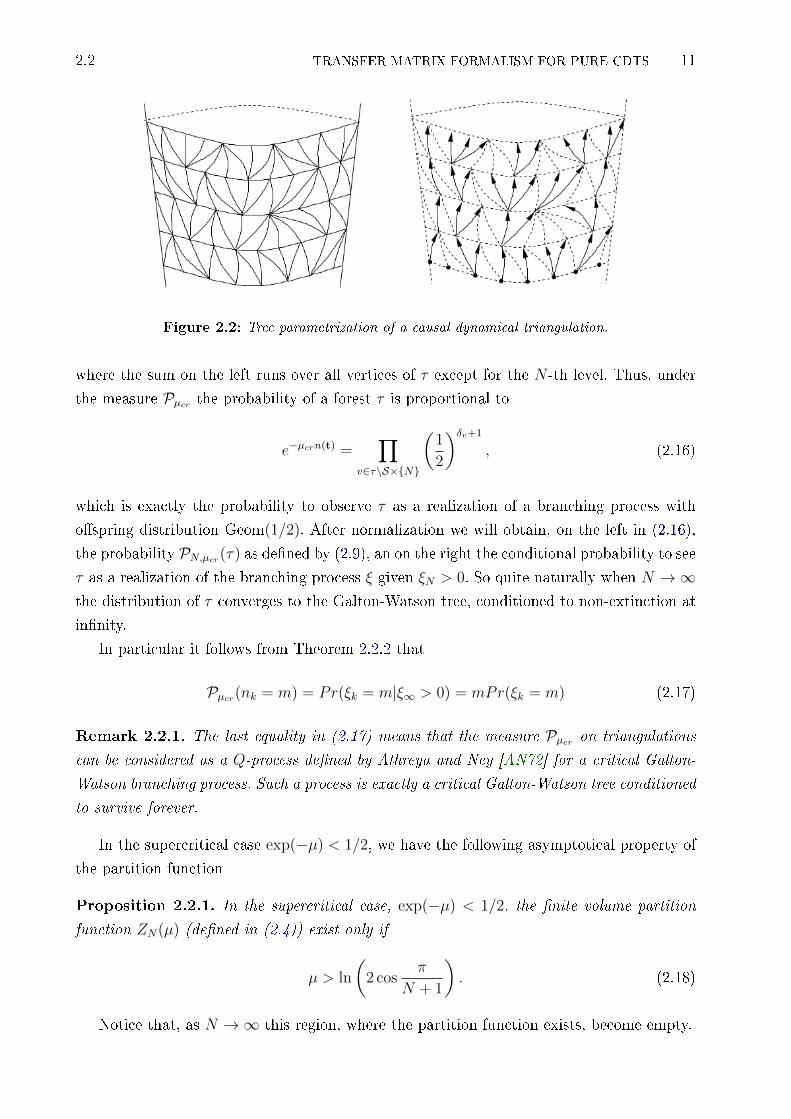
Given a triangulation t ∈ LTN , dene the subgraph τ ⊂ t by taking, for each vertex
v ∈ t , the leftmost edge going from v downwards (see g. 1). The graph thus obtained is a
spanning forest of t , and moreover, if one associates with each vertex of τ it is height in t
then t can be completely reconstructed knowing τ . We call τ the tree parametrization of t.
For every vertex v ∈ τ denote by δv it is out-degree, i.e. the number of edges of τ going
from v upwards. Comparing the out-degrees in τ to the number of vertical edges in t ,
and comparing the latter to the total number of triangles n(t), it is not hard to obtain the
identity ∑v∈τ\S×N
(δv + 1) = n(t), (2.15)
2.2 TRANSFER MATRIX FORMALISM FOR PURE CDTS 11
Figure 2.2: Tree parametrization of a causal dynamical triangulation.
where the sum on the left runs over all vertices of τ except for the N -th level. Thus, under
the measure Pµcr the probability of a forest τ is proportional to
e−µcrn(t) =∏
v∈τ\S×N
(1
2
)δv+1
, (2.16)
which is exactly the probability to observe τ as a realization of a branching process with
ospring distribution Geom(1/2). After normalization we will obtain, on the left in (2.16),
the probability PN,µcr(τ) as dened by (2.9), an on the right the conditional probability to see
τ as a realization of the branching process ξ given ξN > 0. So quite naturally when N →∞the distribution of τ converges to the Galton-Watson tree, conditioned to non-extinction at
innity.
In particular it follows from Theorem 2.2.2 that
Pµcr(nk = m) = Pr(ξk = m|ξ∞ > 0) = mPr(ξk = m) (2.17)
Remark 2.2.1. The last equality in (2.17) means that the measure Pµcr on triangulations
can be considered as a Q-process dened by Athreya and Ney [AN72] for a critical Galton-
Watson branching process. Such a process is exactly a critical Galton-Watson tree conditioned
to survive forever.
In the supercritical case exp(−µ) < 1/2, we have the following asymptotical property of
the partition function
Proposition 2.2.1. In the supercritical case, exp(−µ) < 1/2, the nite volume partition
function ZN(µ) (dened in (2.4)) exist only if
µ > ln
(2 cos
π
N + 1
). (2.18)
Notice that, as N →∞ this region, where the partition function exists, become empty.

12 TWO-DIMENSIONAL CAUSAL DYNAMICAL TRIANGULATIONS 2.2
Remark 2.2.2. The inequality in (2.18) means that if µ < ln 2 then there exists N0 ∈ Nsuch that the partition function ZN(µ) = +∞ whenever N > N0. Moreover, the Gibbs
distribution PN,µ on triangulations with periodic boundary conditions cannot be dened by
using the standard formula with PN,µ as a normalising denominator, consequently, there is
no limiting probability measure Pµ.

Chapter 3
Transfer matrix formalism for Ising
model coupled to two-dimensional CDT
In this chapter we introduce a transfer matrix formalism for the (annealed) Ising model
coupled two-dimensional CDTs. Using the Krein-Rutman theory of positivity preserving
operators we study several properties of the emerging transfer matrix. In particular, we
determine regions in the quadrant of parameters β, µ > 0 where the innite-volume free
energy converges, yields results on the convergence and asymptotic properties of the partition
function and Gibbs measure. This is a rst approach for study the Ising model coupled two-
dimensional CDTs.
3.1 The model
Let t = (t(0), t(1), . . . , t(N − 1)) be a triangulation of CN , where t(i) is a causal trian-
gulation of the strip S × [i, i + 1]. The triangles forming the causal triangulation t(i) are
denoted by t(i, j), 1 ≤ j ≤ n(t(i)) where, n(t(i)) stands for the number of triangles in
the triangulation t(i). The enumeration of these triangles starts with what we call the root
triangle in t(i) (see Chapter 2).
Now, with any triangle from a triangulation t we associate a spin taking values ±1. An
N -strip conguration of spins is represented by a collection
σ = (σ(0),σ(1), . . . ,σ(N − 1))
where σ(i) = σ(t(i)) is a conguration of spins σ(i, j) over triangles t(i, j) forming a trian-
gulation t(i), 1 ≤ j ≤ n(t(i)). We will say that a single-strip conguration of spins σ(i) is
supported by a triangulation t(i) of strip S × [i, i+ 1]. We consider a usual (ferromagnetic)
Ising-type energy where two spins σ(i, j) and σ(i′, j′) interact if their supporting triangles
t(i, j), t(i′, j′) share a common edge; such triangles are called nearest neighbors, and this
property is reected in the notation 〈σ(i, j), σ(i′, j′)〉, where we require 0 ≤ i ≤ i′ ≤ N − 1.
Thus, in our model each spin has three neighbors. Moreover, a pair 〈σ(i, j), σ(i′, j′)〉 can
13

14 TRANSFER MATRIX FORMALISM FOR ISING MODEL COUPLED TO
TWO-DIMENSIONAL CDT 3.1
only occur for i′− i ≤ 1 or i = 0, i′ = N − 1. Formally, the Hamiltonian of the model reads:
H(σ) = −∑
〈σ(i,j),σ(i′,j′)〉
σ(i, j)σ(i′, j′). (3.1)
We will use the following decomposition:
H(σ) =N−1∑i=0
H(σ(i)) +N−1∑i=0
V (σ(i),σ(i+ 1)), (3.2)
where we assume that σ(0) ≡ σ(N) (the periodic spatial boundary condition). Here H(σ(i))
represents the energy of the conguration σ(i):
H(σ(i)) = −∑
〈σ(i,j),σ(i,j′)〉
σ(i, j)σ(i, j′). (3.3)
Further, V (σ(i),σ(i+1)) is the energy of interaction between neighboring triangles belonging
to the adjacent strips S × [i, i+ 1] and S × [i+ 1, i+ 2]:
V (σ(i),σ(i+ 1)) = −∑
〈σ(i,j),σ(i+1,j′)〉
σ(i, j)σ(i+ 1, j′). (3.4)
The partition function for the (annealed) N -strip Ising model coupled to CDT, at the
inverse temperature β > 0 and for the cosmological constant µ, is given by
ΞN(µ, β) =∑
(t(0),...,t(N−1))
exp−µ
N−1∑i=0
n(t(i))
(3.5)
×∑
(σ(0),...,σ(N−1))
N−1∏i=0
exp−βH(σ(i))− βV (σ(i),σ(i+ 1))
.
Here n(t(i)) stands for the number of triangles in the triangulation t(i). Like before, the
formula
ΞN(µ, β) = tr KN (3.6)
gives rise to a transfer matrix K with entriesK((t,σ), (t′,σ′)) labelled by pairs (t,σ), (t′,σ′)
representing triangulations of a single strip (say, S × [0, 1]) and their supported spin cong-
urations which are positioned next to each other. Formally,
K((t,σ), (t′,σ′)) = 1t∼t′ exp−µ
2(n(t) + n(t′))
(3.7)
× exp−β
2
(H(σ) +H(σ′)
)− βV (σ,σ′)
.
As earlier, n(t) and n(t′) are the numbers of triangles in the triangulations t and t′. The
indicator 1t∼t′ means that the triangulations t, t′ have to be consistent with each other in the

3.1 THE MODEL 15
above sense: the number of down-triangles in t should equal the number of up-triangles in
t′, and an upper-marked edge in t should coincide with a lower-marked edge in triangulation
t′. It means that the pair (t, t′) forms a CDT for the strip S × [0, 2].
We would like to stress that the trace tr KN in (3.6) is understood as the matrix trace,
i.e., as the sum∑
t,σK(N)((t,σ), (t,σ)) of the diagonal entries K(N)((t,σ), (t,σ)) of the
matrix KN . (Indeed, in what follows, the notation tr is used for the matrix trace only.)
Our aim will be to verify that the matrix trace in (3.6) can be replaced with an operator
trace invoking the eigenvalues of K in a suitable linear space (see next section).
As before, we can introduce the N -strip Gibbs probability distribution associated with
formula (3.5):
PN((t(0),σ(0)), . . . , (t(N − 1),σ(N − 1))
)(3.8)
=1
Ξ(µ, β)
N−1∏i=0
exp−µn(t(i))− βH(σ(i))− βV (σ(i),σ(i+ 1))
.
Consider several special cases of interest.
The case β ≈ 0. This is the rst term of the so-called high temperature expansion [AAL99].
Here one has
Ξ(µ, 0) =∑
(t(0),...,t(N−1))
exp−µ
N−1∑i=0
n(t(i)) ∑
(σ(0),...,σ(N−1))
1
=∑
n0≥1,...,nN−1≥1
exp−2(µ− ln 2)
N−1∑i=0
niN−1∏
i=0
(ni + ni+1 − 1
ni − 1
)
= ZN(µ− ln 2); cf. (2.4).
The condition µ − ln 2 > ln 2 which guarantees properties listed in Lemma 2.2.3 and
Theorem 2.2.1 resuls in
µ > 2 ln 2. (3.9)
Thus, Eqn. (3.9) yields a sub-criticality condition when β = 0.
The case β ≈ ∞. Observe that for any triangulation t = (t(0), . . . , t(N − 1)) there are two
ground states: all spins +1 and all spins −1, with the overall energy equals minus three
half times the total number of triangles: −3/2∑N−1
i=0 n(t(i)). Discarding all other spin
congurations, we obtain that
Ξ(µ, β) > Ξ∗(µ, β)
16 TRANSFER MATRIX FORMALISM FOR ISING MODEL COUPLED TO
TWO-DIMENSIONAL CDT 3.1
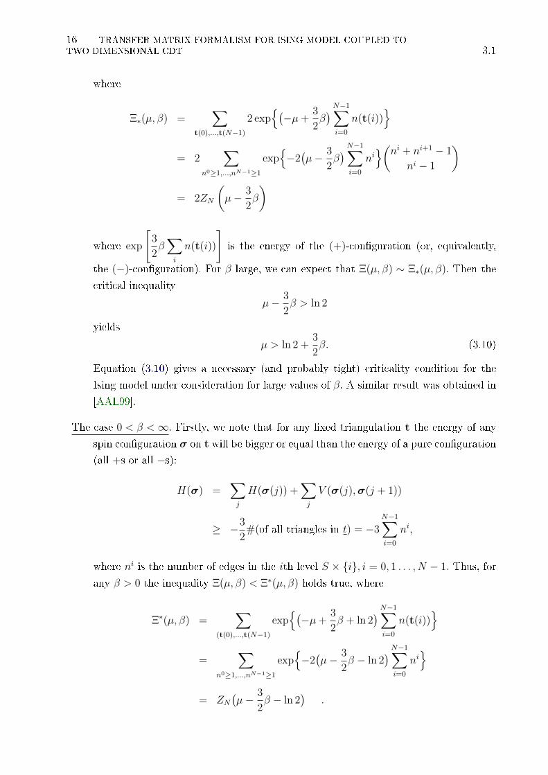
where
Ξ∗(µ, β) =∑
t(0),...,t(N−1)
2 exp(−µ+
3
2β)N−1∑i=0
n(t(i))
= 2∑
n0≥1,...,nN−1≥1
exp−2(µ− 3
2β)N−1∑i=0
ni(ni + ni+1 − 1
ni − 1
)
= 2ZN
(µ− 3
2β
)
where exp
[3
2β∑i
n(t(i))
]is the energy of the (+)-conguration (or, equivalently,
the (−)-conguration). For β large, we can expect that Ξ(µ, β) ∼ Ξ∗(µ, β). Then the
critical inequality
µ− 3
2β > ln 2
yields
µ > ln 2 +3
2β. (3.10)
Equation (3.10) gives a necessary (and probably tight) criticality condition for the
Ising model under consideration for large values of β. A similar result was obtained in
[AAL99].
The case 0 < β <∞. Firstly, we note that for any xed triangulation t the energy of any
spin conguration σ on t will be bigger or equal than the energy of a pure conguration
(all +s or all −s):
H(σ) =∑j
H(σ(j)) +∑j
V (σ(j),σ(j + 1))
≥ −3
2#(of all triangles in t) = −3
N−1∑i=0
ni,
where ni is the number of edges in the ith level S × i, i = 0, 1 . . . , N − 1. Thus, for
any β > 0 the inequality Ξ(µ, β) < Ξ∗(µ, β) holds true, where
Ξ∗(µ, β) =∑
(t(0),...,t(N−1)
exp(−µ+
3
2β + ln 2
)N−1∑i=0
n(t(i))
=∑
n0≥1,...,nN−1≥1
exp−2(µ− 3
2β − ln 2
)N−1∑i=0
ni
= ZN(µ− 3
2β − ln 2
).

3.2 THE TRANSFER-MATRIX K AND ITS POWERS KN 17
Hence, the inequality
µ− 3
2β − ln 2 > ln 2 or µ > 2 ln 2 +
3
2β (3.11)
provides a sucient condition for subcriticality of the Ising model under consideration.
3.2 The transfer-matrix K and its powers KN
The main results of this chapter are summarized in Lemma 3.2.1 and Theorems 3.2.1
and 3.2.2 below.
Let us start with a statement (see Proposition 3.2.1 below) which merely re-phrases
standard denitions and explains our interest in the matrices K, KT, KTK, KKT and their
powers. Cf. Denition 2.2.2 on p.83, Denition 2.4.1 on p.101, Lemma 2.3.1 on p.85 and
Theorem 3.3.13 on p.139 in [Rin71]). See Appendix A for a short review.
We treat the transfer-matrix K and its transpose KT as linear operators in the Hilbert
space `2T−C (the subscript T-C refers to triangulations and spin-congurations). The space
`2T−C is formed by functions ψ = ψ(t,σ) with the argument (t,σ) running over single-strip
triangulations and supported congurations of spins, with the scalar product 〈ψ′,ψ′′〉T−C =∑t,σ ψ
′(t,σ)ψ′′(t,σ) and the induced norm ‖ψ‖T−C. The action of K in `2T−C, in the basis
formed by Dirac's delta-vectors δ(t,σ), is determined by
(Kψ
)(t,σ) =
∑t′,σ′
K((t,σ), (t′,σ′))ψ(t′,σ′); (3.12)
in following we use the notation K, KT, etc., for the matrices and the corresponding operators
in `2T−C. Accordingly, the symbols ‖K‖T−C, ‖KT‖T−C etc. refer to norms in `2
T−C.
Given n = 1, 2, . . ., suppose that the operator Kn (respectively,(KT)n) is of trace class
(see denition in Appendix A). Then the following series absolutely converges:
∑j
Λ(n)j
(respectively,
∑j
Λ∗(n)j
), (3.13)
where Λ(n)j (Λ∗
(n)j ) runs through the eigenvalues of Kn ((KT)n), counted with their multi-
plicities. In this case the sum (3.13) is called the operator trace of Kn (respectively, (KT)n)
in `2T−C. We adopt an agreement that the eigenvalues in (3.13) are listed in the decreasing
order of their moduli, beginning with Λ(n)0 (Λ∗
(n)0 ).
Set |Kn| =√
(KT)n Kn and∣∣(KT
)n∣∣ =√
Kn (KT)n.
18 TRANSFER MATRIX FORMALISM FOR ISING MODEL COUPLED TO
TWO-DIMENSIONAL CDT 3.2
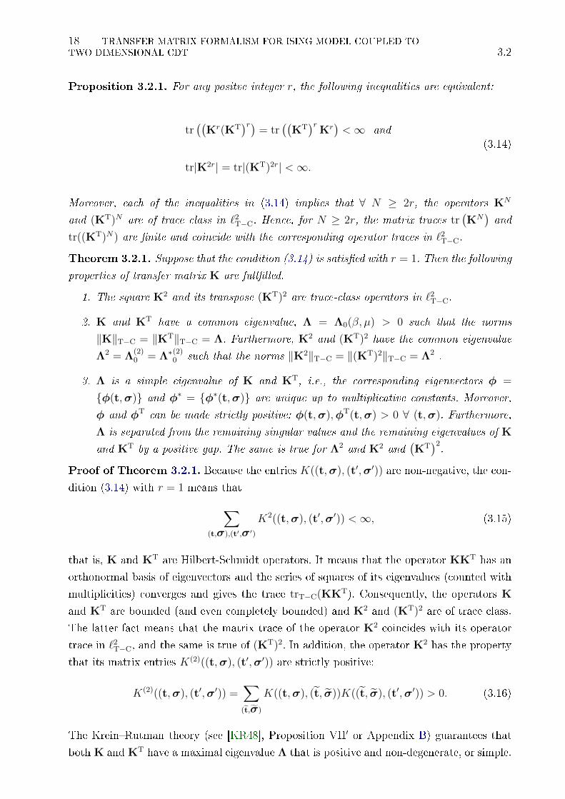
Proposition 3.2.1. For any positve integer r, the following inequalities are equivalent:
tr((
Kr(KT)r)
= tr((
KT)r
Kr)<∞ and
tr|K2r| = tr|(KT)2r| <∞.
(3.14)
Moreover, each of the inequalities in (3.14) implies that ∀ N ≥ 2r, the operators KN
and (KT)N are of trace class in `2T−C. Hence, for N ≥ 2r, the matrix traces tr
(KN)and
tr((KT)N) are nite and coincide with the corresponding operator traces in `2T−C.
Theorem 3.2.1. Suppose that the condition (3.14) is satised with r = 1. Then the following
properties of transfer matrix K are fulllled.
1. The square K2 and its transpose (KT)2 are trace-class operators in `2T−C.
2. K and KT have a common eigenvalue, Λ = Λ0(β, µ) > 0 such that the norms
‖K‖T−C = ‖KT‖T−C = Λ. Furthermore, K2 and (KT)2 have the common eigenvalue
Λ2 = Λ(2)0 = Λ∗
(2)0 such that the norms ‖K2‖T−C = ‖(KT)2‖T−C = Λ2 .
3. Λ is a simple eigenvalue of K and KT, i.e., the corresponding eigenvectors φ =
φ(t,σ) and φ∗ = φ∗(t,σ) are unique up to multiplicative constants. Moreover,
φ and φT can be made strictly positive: φ(t,σ),φT(t,σ) > 0 ∀ (t,σ). Furthermore,
Λ is separated from the remaining singular values and the remaining eigenvalues of K
and KT by a positive gap. The same is true for Λ2 and K2 and(KT)2.
Proof of Theorem 3.2.1. Because the entries K((t,σ), (t′,σ′)) are non-negative, the con-
dition (3.14) with r = 1 means that∑(t,σ),(t′,σ′)
K2((t,σ), (t′,σ′)) <∞, (3.15)
that is, K and KT are Hilbert-Schmidt operators. It means that the operator KKT has an
orthonormal basis of eigenvectors and the series of squares of its eigenvalues (counted with
multiplicities) converges and gives the trace trT−C(KKT). Consequently, the operators K
and KT are bounded (and even completely bounded) and K2 and (KT)2 are of trace class.
The latter fact means that the matrix trace of the operator K2 coincides with its operator
trace in `2T−C, and the same is true of (KT)2. In addition, the operator K2 has the property
that its matrix entries K(2)((t,σ), (t′,σ′)) are strictly positive:
K(2)((t,σ), (t′,σ′)) =∑(t,σ)
K((t,σ), (t, σ))K((t, σ), (t′,σ′)) > 0. (3.16)
The KreinRutman theory (see [KR48], Proposition VII′ or Appendix B) guarantees that
both K and KT have a maximal eigenvalue Λ that is positive and non-degenerate, or simple.

3.2 THE TRANSFER-MATRIX K AND ITS POWERS KN 19
That is, the eigenvector φ of K and the eigenvector φ∗ of KT corresponding with Λ are
unique up to multiplication by a constant, and all entries φ(t,σ) and φ∗(t,σ) are non-
zero and have the same sign. In other words, the entries φ(t,σ) and φ∗(t,σ) can be made
positive. The spectral gaps are also consequences of the above properties.
Set:
λ(µ, β) = c2 (m2 + 1) (cosh 2β)
(1 +
√1− 1
(cosh 2β)2
(m2 − 1)2
(m2 + 1)2
)(3.17)
where c and m are determined by
c =exp(β − µ)
e2β(1− exp(β − µ))2 − e−2µ(3.18)
m = e2β + (1− e4β) exp (−(β + µ)). (3.19)
Lemma 3.2.1. For any β, µ > 0 such that
λ(µ, β) < 1, (3.20)
the condition (3.14) is satised for r = 1:
tr(KKT) = tr(KTK) <∞ and tr|K2| = tr|(KT)2| <∞, (3.21)
implying the assertions of Proposition 3.2.1 and Theorem 3.2.1. Moreover, the condition
(3.14) implies (3.20)
Proof of Lemma 3.2.1. By denition the trace (3.21) we need to calculate the series
tr(KTK) =∑(t,σ)
KTK((t,σ), (t,σ))
=∑
(t,σ),(t′,σ′)K((t,σ), (t′,σ′))K((t,σ), (t′,σ′))
=∑
(t,σ),(t′,σ′)K2((t,σ), (t′,σ′)). (3.22)
A single-strip triangulation t consists of up- and down-triangles. Accordingly, it is con-
venient to employ new labels for spins: if a triangle t(l) is an lth up-triangle then we denote
it by tlup; the corresponding spin σ(j) will be denoted by σlup. Similarly, if t(j) is an lth
down-triangle then we denote it by tldo; the spin σ(j) will be denoted by σldo. Consequently,
the triangulation t and its supported spin-conguration σ are represented as
t := (tup, tdo) and σ := (σup,σdo).
20 TRANSFER MATRIX FORMALISM FOR ISING MODEL COUPLED TO
TWO-DIMENSIONAL CDT 3.2
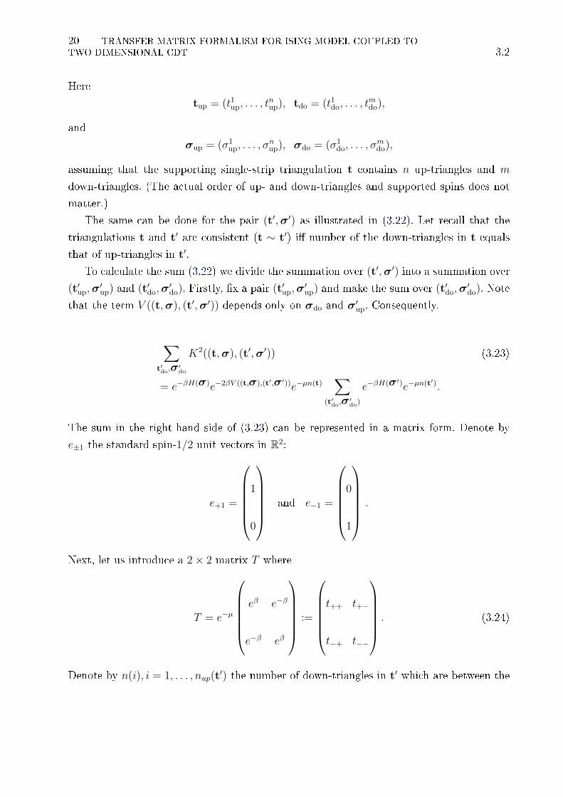
Here
tup = (t1up, . . . , tnup), tdo = (t1do, . . . , t
mdo),
and
σup = (σ1up, . . . , σ
nup), σdo = (σ1
do, . . . , σmdo),
assuming that the supporting single-strip triangulation t contains n up-triangles and m
down-triangles. (The actual order of up- and down-triangles and supported spins does not
matter.)
The same can be done for the pair (t′,σ′) as illustrated in (3.22). Let recall that the
triangulations t and t′ are consistent (t ∼ t′) i number of the down-triangles in t equals
that of up-triangles in t′.
To calculate the sum (3.22) we divide the summation over (t′,σ′) into a summation over
(t′up,σ′up) and (t′do,σ
′do). Firstly, x a pair (t′up,σ
′up) and make the sum over (t′do,σ
′do). Note
that the term V ((t,σ), (t′,σ′)) depends only on σdo and σ′up. Consequently,
∑t′do,σ′do
K2((t,σ), (t′,σ′)) (3.23)
= e−βH(σ)e−2βV ((t,σ),(t′,σ′))e−µn(t)∑
(t′do,σ′do)
e−βH(σ′)e−µn(t′).
The sum in the right-hand side of (3.23) can be represented in a matrix form. Denote by
e±1 the standard spin-1/2 unit vectors in R2:
e+1 =
1
0
and e−1 =
0
1
.
Next, let us introduce a 2× 2 matrix T where
T = e−µ
eβ e−β
e−β eβ
:=
t++ t+−
t−+ t−−
. (3.24)
Denote by n(i), i = 1, . . . , nup(t′) the number of down-triangles in t′ which are between the

3.2 THE TRANSFER-MATRIX K AND ITS POWERS KN 21
ith and (i+ 1)th up-triangles in t′. Let nup(t′) = k then
∑t′do,σ′do
e−βH(σ′)e−µn(t′) =∑
n(i)≥0:∑i n(i)≥1
k∏l=1
(eTσ′lup
T n(l)+1eσ′l+1up
)
=k∏l=1
(eTσ′lup
Meσ′l+1up
)−
k∏l=1
(eTσ′lup
Teσ′l+1up
)(3.25)
where the matrix M is the sum of the geometric progression
M =∞∑n=1
T n :=
m++ m+−
m−+ m−−
. (3.26)
Using the same procedure we can obtain the sum over all up-triangles into the triangulation
t. The only dierence is the existence of marked up-triangle in the strip: let as before
nup(t′) = ndo(t) = k then
∑tup,σup
e−βH(σ)e−µn(t) =k−1∏l=1
(eTσlupMeσl+1
up
)(eTσkupM2eσ1
up
)(3.27)
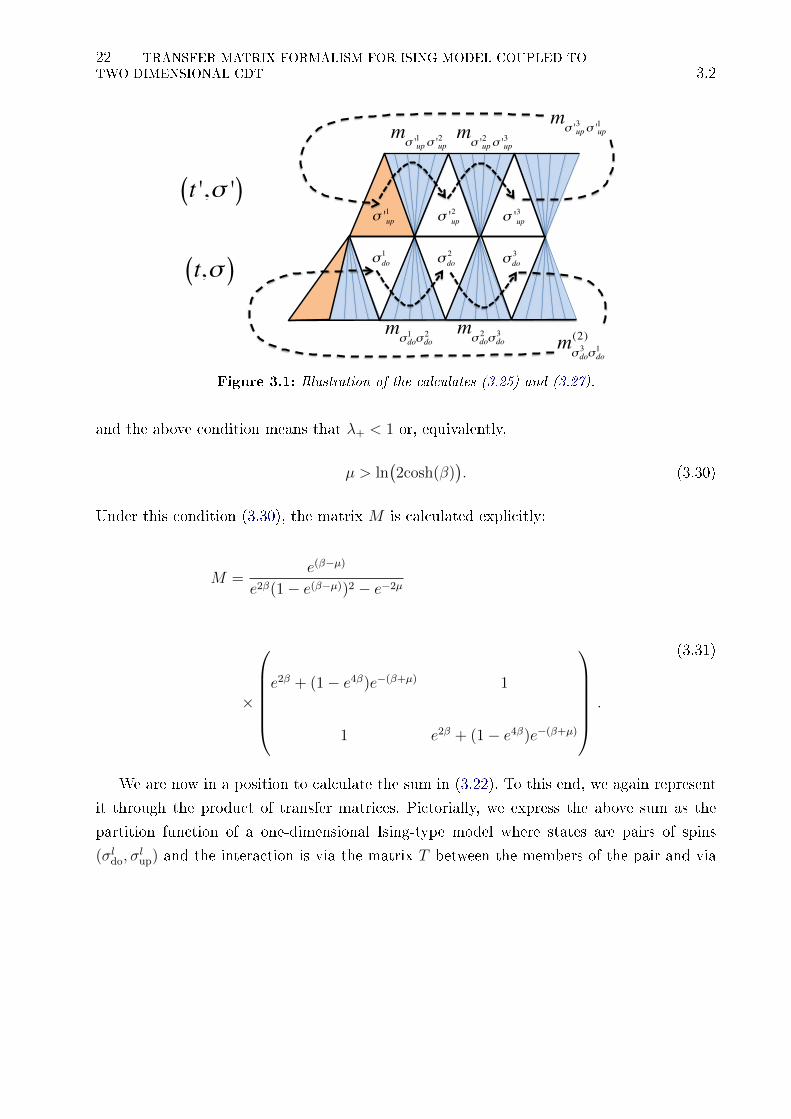
See Figure 3.1 for illustration of these calculations (3.25) and (3.27). Further, supposing the
existence of the matrix M and using (3.25) and (3.27) we obtain the following:∑tup,σup
∑t′do,σ′do
K2((t,σ), (t′,σ′)) = e−2βV ((tdo,σdo),(t′up,σ′up))
×∑
tup,σup
e−βH(σ)e−µn(t)∑
(t′do,σ′do)
e−βH(σ′)e−µn(t′)
= e−2βV ((tdo,σdo),(t′up,σ′up))
×[ k∏l=1
(eTσ′lup
Meσ′l+1up
) k−1∏l=1
(eTσldoMeσl+1
do
)(eTσkupM2eσ1
up
)−
k∏l=1
(eTσ′lup
Teσ′l+1up
) k−1∏l=1
(eTσldoMeσl+1
do
)(eTσkupM2eσ1
up
)]. (3.28)
Necessary and sucient condition for the convergence of the matrix series for M is that
the maximal eigenvalue of matrix T is less then 1. The eigenvalues of T are
λ± = e(β−µ) ± e−(β+µ), (3.29)
22 TRANSFER MATRIX FORMALISM FOR ISING MODEL COUPLED TO
TWO-DIMENSIONAL CDT 3.2
t ',σ '( )
t,σ( )
σ 'up1
σ do1
σ 'up2
σ do2
σ 'up3
σ do3
mσ 'up1 σ 'up
2 mσ 'up2 σ 'up
3
mσ 'up3 σ 'up
1
mσ do1 σ do
2 mσ do2 σ do
3 mσ do3 σ do
1(2)
Figure 3.1: Illustration of the calculates (3.25) and (3.27).
and the above condition means that λ+ < 1 or, equivalently,
µ > ln(2cosh(β)
). (3.30)
Under this condition (3.30), the matrix M is calculated explicitly:
M =e(β−µ)
e2β(1− e(β−µ))2 − e−2µ
×
e2β + (1− e4β)e−(β+µ) 1
1 e2β + (1− e4β)e−(β+µ)
.
(3.31)
We are now in a position to calculate the sum in (3.22). To this end, we again represent
it through the product of transfer matrices. Pictorially, we express the above sum as the
partition function of a one-dimensional Ising-type model where states are pairs of spins
(σldo, σlup) and the interaction is via the matrix T between the members of the pair and via

3.2 THE TRANSFER-MATRIX K AND ITS POWERS KN 23
matrix M between neighboring pairs. More precisely, dene the following 4× 4 matrices:
Q =
e2βm++m++ m++m+− m+−m++ e2βm+−m+−
m++m−+ e−2βm++m−− e−2βm+−m−+ m+−m−−
m−+m++ e−2βm−+m+− e−2βm−−m++ m−−m+−
e2βm−+m−+ m−+m−− m−−m−+ e2βm−−m−−
(3.32)
Qm =
e2βm++m(2)++ m++m
(2)+− m+−m
(2)++ e2βm+−m
(2)+−
m++m(2)−+ e−2βm++m
(2)++ e−2βm+−m
(2)−+ m+−m
(2)−−
m−+m(2)++ e−2βm−+m
(2)+− e−2βm−−m
(2)++ m++m
(2)++
e2βm−+m(2)−+ m−+m
(2)−− m−−m
(2)−+ e2βm−−m
(2)−−
(3.33)
Qt =
e2βt++m++ t++m+− t+−m++ e2βt+−m+−
t++m−+ e−2βt++m−− e−2βt+−m−+ t+−m−−
t−+m++ e−2βt−+m+− e−2βt−−m++ t−−m+−
e2βt−+m−+ t−+m−− t−−m−+ e2βt−−m−−
(3.34)
Qtm =
e2βt++m(2)++ t++m
(2)+− t+−m
(2)++ e2βt+−m
(2)+−
t++m(2)−+ e−2βt++m
(2)++ e−2βt+−m
(2)−+ t+−m
(2)−−
t−+m(2)++ e−2βt−+m
(2)+− e−2βt−−m
(2)++ t++m
(2)++
e2βt−+m(2)−+ t−+m
(2)−− t−−m
(2)−+ e2βt−−m
(2)−−
(3.35)

24 TRANSFER MATRIX FORMALISM FOR ISING MODEL COUPLED TO
TWO-DIMENSIONAL CDT 3.2
where mij,m(2)ij and ti,j (i, j ∈ −,+) are elements of the matrices M,M2, and T respec-
tively.
Now for the sum under consideration (3.22) we obtain using representation (5.53)∑(t,σ),(t′,σ′)
K2((t,σ), (t′,σ′)) =∑
(tdo,σdo),(t′up,σ′up)
e−2βV ((tdo,σdo),(t′up,σ′up))
×
[k∏l=1
(eTσ′lup
Meσ′l+1up
) k−1∏l=1
(eTσldoMeσl+1
do
)(eTσkupM2eσ1
up
)−
k∏l=1
(eTσ′lup
Teσ′l+1up
) k−1∏l=1
(eTσldoMeσl+1
do
)(eTσkupM2eσ1
up
)]
= tr(( ∞∑
k=0
Qk)Qm
)− tr
(( ∞∑k=1
Qkt
)Qtm
). (3.36)
By the construction the matrix Q is greater then Qt elementwise. Thus the eigenvalue of
matrixQ is greater than the eigenvalue of the matrixQt (it follows from the Perron-Frobenius
theorem). Therefore the necessary and sucient condition for the convergence in (3.22) is
that the largest eigenvalue of Q is less than 1. It is possible to calculate its eigenvalue
analytically. In order to express the eigenvalues of Q it is convinient to use notations (3.18)
and (3.19). In this notations the matrix M , i.e. (3.31), is represented as following
M = c
m 1
1 m
.
The equations for the eigenvalues of Q are:
λ1 = c2eβ(m2 − 1)
λ2 = c2e−β(m2 − 1)
λ3 = c2(m2 + 1)(cosh β)
(1−
√1− (m2 − 1)2
(cosh β)2(m2 + 1)2
)
λ4 = c2(m2 + 1)(cosh β)
(1 +
√1− (m2 − 1)2
(cosh β)2(m2 + 1)2
)
A straightforward inspection conrms that the largest eigenvalue is given by λ4. The con-
dition λ4 < 1 coincides with (3.20). Finally, using matrices Q,Qm (see formulas (3.32) and
(3.33)) with positive entries and of size 4× 4, we have the following representation of 3.22
tr(KKT) = tr((∑
k≥1
Qk)Qm
)+ . . . .

3.3 DISCUSSION AND OUTLOOK 25
The convergence of the matrix series∑
k≥1Qk is equivalent to the condition that the maximal
eigenvalue of the matrix Q is less then 1. This is exactly the condition (3.20). This completes
the proof of Lemma 3.2.1.
Theorem 3.2.2. Under condition (3.20), the following limit holds:
limN→∞
1
Nlog ΞN(β, µ) = log Λ. (3.37)
Moreover, as N → ∞, the N-strip Gibbs measure PN (see Eqn (5.9)) converges weakly to
a limiting probability distribution P that is represented by a positive recurrent Markov chain
with states (t,σ), the transition matrix
P = P ((t,σ), (t′,σ′)) and the invariant distribution π = π(t,σ) where
P ((t,σ), (t′,σ′)) =K((t,σ), (t′,σ′))φ(t′,σ′)
Λφ(t,σ)
π(t,σ) = φ(t,σ)φT(t,σ)/⟨φ,φT
⟩T−C
with the norm∥∥φ∥∥2
T−C=∑
t,σ φ(t,σ)2.
Proof of Theorem 3.2.2. The spectral gap for K implies that ∀ ψ ∈ `2T−C, we have the
convergence
limN→∞
1
ΛNKNψ = (〈ψ,φ〉T−C)φ
in the norm of space `2T−C. Moreover, let Π denote the operator of projection to the subspace
spanned by the eigenvectors of K dierent from φ. Then
1
Λ‖ΠKP‖T−C < 1 =⇒ lim
N→∞
1
ΛN
∥∥∥(ΠKP)N∥∥∥
T−C= 0.
In turn, this implies that
1
Nlog ΞN(µ, β) =
1
Nlog trT−CKN → log Λ.
Convergence of the Gibbs measure PN follows as a corollary.
3.3 Discussion and outlook
This chapter makes a step towards determining the subcriticality domain for an Ising-
type model coupled to two-dimensional causal dynamical triangulations (CDT). In doing
so we employ transfer-matrix techniques and in particular the Krein-Rutman theorem. We
complement the discussion of the previous sections with the following two concluding re-
marks:

26 TRANSFER MATRIX FORMALISM FOR ISING MODEL COUPLED TO
TWO-DIMENSIONAL CDT 3.3
Remark 1. It is instructive to summarise the logical structure of the argument establishing
Lemma 3.2.1 and Theorems 3.2.1 and 3.2.2:
• First, (3.21) holds i condition (3.20) holds: see the proof of Lemma 3.2.1.
• Next, (3.21) implies that K is a HilbertSchmidt operator and K2 is a trace class
operator in `2T−C.
• The last fact, together with the property of positivity (3.16), allow us to use the Krein
Rutman theory, deriving all assertions of Theorems 3.2.1 and 3.2.2.
On the other hand, if (3.20) fails (and therefore (3.21) fails), it does not necessarily mean
that the assertions Theorems 3.2.1 and 3.2.2 fail. In other words, we do not claim that the
boundary of the domain of parameters β and µ where the model exhibits uncritical behavior
is given by Eqn. (3.20). Moreover, Figure 3.2 shows the result of a numerical calculation
indicating that the condition (3.20) is worse than (3.11) for (moderately) large values of β.
An apparent condition closer to necessity is the pair of inequalities (3.14) for some (pos-
sibly) large r. This issue needs a further study.
Remark 2. Physical considerations suggest that the critical curve in the (β, g) quarter-
plane would have some predictable patterns of behavior: as a function of β, it would decay
and exhibit a rst-order singularity at a unique point β = βcr ∈ (0,∞).
A plausible conjecture is that the boundary of the critical domain coincides with the locus
of points (β, µ) where Λ looses either the property of positivity or the property of being a
simple eigenvalue. This direction also requires further research.
𝛽 ≈ 0
𝜇
𝛽
𝜆 ≤1
𝜆 ≤1
Figure 3.2: λQ = λ and λT are the maximal eigenvalues of the matrix Q and a related matrix Trespectively. The area above the black curve is where the condition (3.20) holds true.

Chapter 4
FK representation for the Ising model
coupled to CDT
This chapter extends results from before chapter for the (annealed) classical Ising model
coupled to two-dimensional causal dynamical triangulations. Using the Fortuin-Kasteleyn
(FK) representation of quantum Ising models via path integrals, we determine a region in
the quadrant of parameters β, µ > 0 where the critical curve for the classical model can be
located. In particular, we determine a region where the innite-volume Gibbs measure exists
and it is unique, and a region where the nite-volume Gibbs measure has no weak limit (in
fact, does not exist if the volume is large enough). We also provide lower and upper bounds
for the innite-volume free energy.
FK models were introduced by Fortuin and Kasteleyn (see [FK72]). These models have
become an important tool in the study of phase transition for the Ising and Potts model. The
goal of this chapter is to introduce the FK representation of a quantum Ising model coupled to
CDTs via a path integral (see [Aiz94], [Iof09] for an overview), and use this representation for
obtain information of the critical curve. The aforementioned FK representation uses a family
of Poisson point processes and the Lie-Trotter product formula to interpret exponential
sums of operators as random operator products. This representation was originally derived
in [Aiz94].
4.1 The quantum Ising model
In this section we write the classical partition function, over a given triangulation, by
using ingredients of the quantum Ising model.
Henceforth, for simplicity in notation and exposure of the following chapter, we shall
denote a triangle of any triangulation t doing without put the indices i, j as was done in
previous chapter. Thus, in this chapter, the Hamiltonian the (annealed) model is written as
follow
H(σ) = −∑〈t,t′〉
σ(t)σ(t′). (4.1)
27

28 FK REPRESENTATION FOR THE ISING MODEL COUPLED TO CDT 4.1
Here, 〈t, t′〉 stands that triangles t, t′ have a common edge. These triangles are called nearest
neighbor.
Let t = (t(0), t(1), . . . , t(N − 1)) be a causal triangulation of CN with periodical spa-
tial boundary condition (see Figure 3.1 (b)). Let ∆(t) denote the set of triangles of the
triangulation t.
We dene Ω(t) to be set of all spin congurations supported by the triangles of t, i.e.,
Ω(t) = −1,+1∆(t). Let Zβ,tN be the partition function of the Ising model on the CDT t,
at inverse temperature β > 0
Zβ,tN =∑σ∈Ω(t)
exp−βH(σ), (4.2)
where H(σ) represents the energy of conguration σ ∈ Ω(t), dened by the formula (4.1).
The quantum Ising model on a causal triangulation t is dened as follows.
Let
σz =
1 0
0 −1
(4.3)
be the Pauli matrix with their corresponding eigenvectors
φ+1 =
1
0
and φ−1 =
0
1
. (4.4)
In the quantum lenguage spins values ±1 are understood as eigenvalues of Pauli matrix.
Notice that σzφν = νφν for ν = ±1.
To each triangle t ∈ ∆(t) we associate a spin taking values φ+1 and φ−1. Thus, the space
of all such spin congurations on t is dene as the real vector space Xt =⊗
t∈∆(t) R2, where⊗stands for the tensor product. Notice that Xt is a real vector space of dimension 2 to the
n(t) power: dim(Xt) = 2n(t).
For each classical conguration σ ∈ Ω(t) we associate the quantum conguration as
tensor products
φσ := ⊗t∈∆(t)φσ(t),
where σ(t) is the spin supported by the triangle t ∈ ∆(t). Notice that there is a one-
one correspondence between Ω(t) and the collection φσσ∈Ω(t). Moreover, the collection of
quantum congurations is a complete orthonormal basis of Xt with respect to the following

4.2 FK REPRESENTATION FOR ISING MODEL COUPLED TO CDT 29
scalar product
〈φσ|φσ′〉 :=∏t∈∆(t)
(φσ(t),φσ′(t)
)2,
where (·, ·)2 is the usual scalar product of R2. With each triangle t ∈ ∆(t) we associate a
linear self-adjoint operator σzt : Xt → Xt which acts as a copy of Pauli matrix σz on the
coordinate of φσ associated to the triangle t of t. That is, for each σ ∈ Ωt,
σztφσ = φσ(t1) ⊗ · · · ⊗(σzφσ(t)
)⊗ · · · = σ(t)φσ. (4.5)
Note that operators σzt , σzt′ commute, and satises
σzt σzt′φσ = σ(t)σ(t′)φσ. (4.6)
The Hamiltonian Ht of the quantum Ising model is a linear self-adjoint operator dened on
Xt:
Ht = −∑〈t,t′〉
σzt σzt′ , (4.7)
where two operators σzt and σzt′ interact if their supporting triangles t, t′ ∈ ∆(t) are nearest
neighbors.
Note that Htφσ = H(σ)φσ. In other words, Ht is a diagonal in the φσ basis, and
corresponding eigenvalues being equal to values of the classical Ising Hamiltonian on cong-
urations σ. This allows write the classical partition function Zβ,tN for Ising model, at inverse
temperature β > 0 associated with triangulation t, as follows
Zβ,tN =∑σ∈Ω(t)
exp−βH(σ) =∑σ∈Ω(t)
〈φσ|e−βHt|φσ〉 = tr(e−βHt
). (4.8)
Finally, using the quantum representation (4.8), the partition function for the N -strip Ising
model coupled to CDT, at the inverse temperature β > 0 and for the cosmological constant
µ, can be written as follows
ΞN(β, µ) =∑t
e−µn(t)tr(e−βHt
). (4.9)
4.2 FK representation for Ising model coupled to CDT
In order to calculate tr(e−βHt
)in (4.9) we will use the FK representation for the Ising
model via path integrals, see [Aiz94, Iof09]. By representation (4.9), the trace tr(e−βHt
)may be expressed in terms of a type of path integral with respect to the continuous random-
cluster model on ∆(t)×[0, β] for any Lorentzian triangulation t (see Proposition 4.2.1 below).
For any pair t, t′ ∈ ∆(t) of nearest neighbor triangles, we associate a Poisson process

30 FK REPRESENTATION FOR THE ISING MODEL COUPLED TO CDT 4.2
ξ〈t,t′〉(s) on the time interval [0, β] with intensity 2. We refer to the process ξ〈t,t′〉 as process
of arrivals of operator K〈t,t′〉 on the interval [0, β], where
K〈t,t′〉 =I + σzt σ
zt′
2. (4.10)
Let ξ be the collection of independent Poisson processes ξ〈t,t′〉 : ξ(s) := ξ〈t,t′〉(s)〈t,t′〉∈Et ,where Et is the set of all pairs of neighbor triangles: Et := 〈t, t′〉 : t, t′ ∈ ∆(t).
Let Pβ,t denote the probability measure associated with the family of Poisson process
ξ. We shall abuse notation by using ξ to denote a realization of process of arrivals ξ(s),
s ∈ [0, β]. By independence there are no simultaneous arrivals Pβ,t-a.s. Thus, a realization ξ
of process of arrivals can be represented by a collection of arrival times sii=1,...,Nξ contained
in [0, β] and its corresponding arrival types L(si) ∈ Et, ξ ≡ si, L(si)i=1,...,Nξ , where Nξ is
the total number of arrivals during the time [0, β].
With a xed realization ξ we associated a family of all possible piecewise constant right-
continuous functions ψξ = ϕ : [0, β] → φσ, having jumps only at arrival times of
ξ. Since Xt is nite dimensional and there are Pβ,t-a.s. nite number of arrivals, we have
|ψξ| <∞, Pβ,t-a.s., where |ψξ| is the total number of functions in the set ψξ.
For each arrival time s of a realization ξ corresponding a unique arrival type L(s) a.s.
Suppose that L(s) = 〈t, t′〉 for t, t′ ∈ ∆(t) nearest neighbor, then KL(s) = K〈t,t′〉 : Xt → Xt.
Let ϕ ∈ ψξ, and denote ϕ(s−) = limt→s− ϕ(t). Notice that the function ϕ ∈ ψξ can be
continuous or not at each arrival time s (see Figure 4.1 below).
arrival ofoperator
arrival ofoperator
Figure 4.1: A trajectory sample associated with a realization ξ = sii=1,...,n. Each trajectory
ϕ ∈ ψξ can be continuous or not at each arrival time s. In this case, at arrival time sk−1 the
trajectory ϕ do not have jump, and at arrival time sk the trajectory ϕ have a jump.
Using the before notation, we have the following proposition.

4.2 FK REPRESENTATION FOR ISING MODEL COUPLED TO CDT 31
Proposition 4.2.1. The matrix elements of the linear operator e−βHt with respect to the
basis φσ are given by
⟨φσ|e−βHt|φσ′
⟩= exp
3
2βn(t)
∫Pβ,t(dξ)
∑ϕ∈ψξ
ϕ(0)=φσ ,ϕ(β)=φσ′
∏s∈ξ
〈ϕ(s−)|KL(s)|ϕ(s)〉, (4.11)
for all t ∈ LTN .
Formula (4.11) was proved in [Aiz94] and [Iof09] for any general nite graph.
With any realization ξ we associate a graph Gξ = (∆ξ, Eξ), where the set of vertices is
∆ξ = ∆(t) and the set of edges Eξ ⊆ Et is dened by following rule: an edge e = 〈t, t′〉 ∈ Etbelong to Eξ if and only if there exist a arrival time s such that the corresponding arrival
type L(s) is 〈t, t′〉 into the realization ξ.
We say that two triangulations t and t′ are connected, denoted by t ↔ t′, if and only if
there exist a path inGξ connecting t and t′. For any t ∈ ∆(t), we suppose that t↔ t. A subset
C ⊆ ∆(t) is called a cluster (maximal connected component) if for any t, t′ ∈ C then t↔ t′,
and t = t′ for any t ∈ C and t′ /∈ C (see Figure 5.1 below). Thus, any realization ξ of the
Poisson process splits ∆(t) into the disjoint union of maximal connected components, i.e., for
any realization ξ there exists k = k(ξ) ∈ 1, . . . , n(t) and sets C1 = C1 . . . , Ck = Ck(ξ) ⊆ ∆(t)
such that
∆(t) =
k(ξ)⋃i=1
Ci,
and Ci ∩ Cj = ∅ for i 6= j, Here k(ξ) is the number of clusters dened by the relation ↔.
Additionally, we dene the cluster Ct of a triangle t by Ct = t′ ∈ ∆(t) : t↔ t′.
Time
Figure 4.2: In this gure, we show the Cluster Ct of a triangle t, and a graphic representation of
relation t↔ t′, where ↔ on right side in the gure, represent arrival times.
Let σ,σ′ ∈ Ω(t) be two congurations and let φσ,φσ′ be the corresponding quantum

32 FK REPRESENTATION FOR THE ISING MODEL COUPLED TO CDT 4.3
conguration. Then, for any 〈t, t′〉 ∈ Et
〈φσ|K〈t,t′〉|φσ′〉 = δσ=σ′δσ(t)=σ(t′). (4.12)
Relation (4.12) implies that, for any realization ξ only constant functions of ψξ contribute to
the sum inside the integral (4.11). Additionally, an arrival of K〈t,t′〉 at arrival time s ∈ [0, β]
imposes an additional condition σ(t) = σ(t′) for contribute to the sum in (4.11). Dene
Ω(t, ξ) = σ ∈ Ω(t) : σ has same sign in each cluster Ci.
Notice that |Ω(t, ξ)| = 2k(ξ), and
∑ϕ∈ψξ
ϕ(0)=ϕ(β)=φσ
∏s∈ξ
〈ϕ(s−)|KL(s)|ϕ(s)〉 =
1 if σ ∈ Ω(t, ξ)
0 if σ /∈ Ω(t, ξ)
(4.13)
As an elementary consequence of (4.13) the following representation for partition function
Zβ,tN holds.
Proposition 4.2.2. Let t ∈ LTN and β > 0. We have that
Zβ,tN = tr(e−βHt
)= exp
3
2βn(t)
∫2k(ξ)Pβ,t(dξ). (4.14)
Proof. The proof is consequence of Proposition 4.2.1 and equation (4.13).
Using the N -strip Gibbs probability distribution PN,µ (introduced in Eqn (2.9)) for pure
CDTs with periodical boundary condition, and substituting (4.14) on the right-hand side
of (4.9) we obtain the FK representation of partition function for the N -strip Ising model
coupled to CDTs, at inverse temperature β > 0 and for the cosmological constant µ
ΞN(β, µ) = ZN(r)∑
t∈LTN
∫2k(ξ)Pβ,t(dξ)
PN,r(t), (4.15)
where r = µ− 32β and ZN(·) is dened by (2.4).
4.3 The main results
This section contains the statement of the main theorems of the present chapter.

4.3 THE MAIN RESULTS 33
Understanding by critical curve of the model the boundary of the domain of parameters β
and µ where the model exhibits subcritical behavior, this chapter makes a rigorous derivation
of a subcriticality domain for an Ising model coupled to two-dimensional CDTs, and we nd
a domain where the tipical innite-volume Gibbs measure there no exists. In Figure 4.3, we
show a region where the critical curve of the model should be located. Formally, we dene
the critical curve as follow: We denote by Gβ,µ the set of Gibbs measures given by the closed
convex hull of the set of weak limits:
Pβ,µ = limN→∞
Pβ,µN , (4.16)
and dene the domain of parameters where the weak limit Gibbs distribution exists
Γ =
(β, µ) ∈ R2+ : Gβ,µ 6= ∅
,
and domain where the weak limit Gibbs distribution exists and it is unique
Γ1 =
(β, µ) ∈ R2+ : |Gβ,µ| = 1
.
It is evident that Γ1 ⊆ Γ. Thus, the critical curve γcr for the Ising model coupled to CDT is
dened by
γcr = ∂Γ1 ∩ R2+. (4.17)
Let λ(β, µ) be given by
λ(β, µ) = c2 (m2 + 1) (cosh 2β)
(1 +
√1− 1
(cosh 2β)2
(m2 − 1)2
(m2 + 1)2
)(4.18)
where c and m are determined by
c =exp(β − µ)
e2β(1− exp(β − µ))2 − e−2µ(4.19)
m = e2β + (1− e4β) exp (−(β + µ)), (4.20)
Remember that identity (4.18) was derived in Chapter 3, Lemma 3.2.1.
We dene the strictly increasing function
ψ(β) = infµ ∈ R+ : λ(β, µ) < 1, for β > 0, (4.21)
34 FK REPRESENTATION FOR THE ISING MODEL COUPLED TO CDT 4.3
and the following set
Σ =
(β, µ) ∈ R2
+ : µ < −3
2β + 2 ln 2
⋃
(β, µ) ∈ R2
+ : µ < −3
2β +
3
2ln(e2β − 1
)+ ln 2
.
Let t1, . . . , tk be triangulations of a single strip S× [0, 1] and σ1, . . . ,σk be their correspond-
ing spin congurations. Given 0 ≤ i1 < · · · < ik ≤ N − 1 we dene the nite-dimensional
cylinder Ci1,...,ik = C(t1,σ1),...,(tk,σk)i1,...,ik
as follows
Ci1,...,ik = (t,σ) : (t(i1),σ(i1)) = (t1,σ1), . . . , (t(ik),σ(ik)) = (tk,σk) (4.22)
Theorem 4.3.1. If (β, µ) ∈ Σ then there exists N0 ∈ N such that the partition func-
tion ΞN(β, µ) = +∞ whenever N > N0. Moreover, the Gibbs distribution Pβ,µN with periodic
boundary conditions cannot be dened by using the standard formula with ΞN(β, µ) as a nor-
malising denominator, consequently, there is no limiting probability measure Pβ,µ as N →∞.
Formally, for any nite-dimensional cylinder Ci1,...,ik we obtain Pβ,µN (Ci1,...,ik) = 0 whenever
N > N0 ≥ maxi1, . . . , ik.
Let β∗1 , β∗2 be positive solution of equations
− 3
2β + 2 ln 2 = −3
2β +
3
2ln(e2β − 1) + ln 2 (4.23)
and3
2β + 2 ln 2 = ψ(β), (4.24)
respectively. Together with results from before chapter (see [HYSZ13] for more details),
Theorem 4.3.1 provides two-side bounds for the critical curve.
Theorem 4.3.2. The critical curve γcr satises the following inequalities.
1. If (β, µ) ∈ γcr and 0 < β < β∗1 , then
−3
2β + 2 ln 2 ≤ µ < ψ(β).
The above bound implies that: For any sequence (βk, µk) ⊂ γcr such that βk → 0,
then limk→∞ µk = 2 ln 2.
2. If (β, µ) ∈ γcr and β∗1 ≤ β < β∗2 , then
3
2ln(e2β − 1)− 3
2β + ln 2 ≤ µ < ψ(β).

4.3 THE MAIN RESULTS 35
0 1 2 3 4 5 6 7 8
0
5
10
15
Figure 4.3: The area above the minimum of the dotted curve I (graph of the function ψ dened in
(4.21)) and dash-dotted line II is where the limiting Gibbs probability measure exists and is unique.
The critical curve lies in the region below the dotted curve I and dash-dotted line II but above the
continuous curve III and dashed line IV.
3. If (β, µ) ∈ γcr and β∗2 ≤ β <∞, then
3
2ln(e2β − 1)− 3
2β + ln 2 ≤ µ <
3
2β + 2 ln 2.
As a by-product of the proof of Theorems 4.3.1 and 4.3.2, using the FK representation
we also nd a lower and upper bound for the innite-volume free energy.
Corollary 4.3.1. If µ >3
2β+2 ln 2, then the free energy for the innite-volume Ising model
coupled to CDTs is nite and satises the following inequalities.
1. If 0 < β <1
3ln 2, then
ln Λ
(µ+
3
2β − ln 2
)≤ lim
N→∞
1
Nln ΞN(β, µ) ≤ ln Λ
(µ− 3
2β − ln 2
).
2. If1
3ln 2 ≤ β <∞, then
ln Λ
(µ− 3
2β
)≤ lim
N→∞
1
Nln ΞN(β, µ) ≤ ln Λ
(µ− 3
2β − ln 2
).
Here Λ(s) is given by (2.10).

36 FK REPRESENTATION FOR THE ISING MODEL COUPLED TO CDT 4.4
For each N ∈ N, we dene the follow set in R2+
ΓN = (β, µ) ∈ R2+ : KN is of trace class in `2
T−C, (4.25)
Γ− =⋂N∈N
ΓN and Γ+ =⋃N∈N
ΓN . (4.26)
Obviously, Γ− ⊂ ΓN ⊂ Γ+, for any N ≥ 1, and Pβ,µN there exist on ΓN . In order to each
N ≥ 1, we dene the N -strip functions fN associated with the partition function for the N
-strip Ising model coupled to CDTs as
fN(β) = infµ ∈ R2+ : (β, µ) ∈ ΓN for β > 0. (4.27)
According to Theorem 3.2.2 in before chapter , Theorem 4.3.2 and Proposition 4.4.4,
given in the Section 4.4.2, implies a similar version of Theorem 3.2.2, as following.
Theorem 4.3.3. For (β, µ) ∈ Γ+ = (β, µ) ∈ R2+ : µ > fT−C(β), the following limit holds:
limN→∞
1
Nln ΞN(β, µ) = ln Λ(β, µ), (4.28)
where Λ(β, µ) is the maximal eigenvalue of K and KT in `2T−C and fT−C is pointwise limit
of the family of functions fN. Consequently, as N → ∞ the N-strip Gibbs measure Pβ,µNconverges weakly to a limiting probability distribution Pβ,µ.
4.4 Proof of Theorem 4.3.1 and 4.3.2
The proof is based on nding of upper and lower bounds for the functions fN , introduced
in (4.27), using the FK representation (4.15) and the asymptotic behaviour of the partition
function ZN(·) for pure CDTs with periodical boundary condition. These bounds with the
Proposition 4.4.1, Proposition 4.4.2 and Proposition 4.4.3, established bounds for the critical
curve.
4.4.1 Proof of Theorem 4.3.1
We need two preparatory results. Let t be a Lorentzian CDT on cylinder CN . Given
1 ≤ i ≤ n(t), we dene the sets
Πi = all realization ξ of process ξ〈t,t′〉 such that k(ξ) = i. (4.29)
4.4 PROOF OF THEOREM ?? AND ?? 37
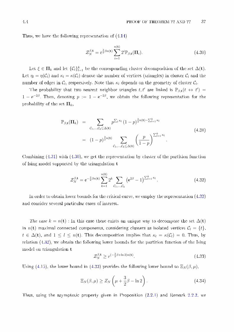
Thus, we have the following representation of (4.14)
Zβ,tN = e32βn(t)
n(t)∑i=1
2iPβ,t(Πi). (4.30)
Let ξ ∈ Πk and let Clkl=1 be the corresponding cluster decomposition of the set ∆(t).
Let ηl = η(Cl) and κl = κ(Cl) denote the number of vertices (triangles) in cluster Cl and the
number of edges in Cl, respectively. Note that κl depends on the geometry of cluster Cl.The probability that two nearest neighbor triangles t, t′ are linked is Pβ,t(t ↔ t′) =
1 − e−2β. Then, denoting p := 1 − e−2β, we obtain the following representation for the
probability of the set Πk,
Pβ,t(Πk) =∑
C1,...,Ck⊆∆(t)
p∑l κl (1− p)
32n(t)−
∑kl=1 κl
= (1− p)32n(t)
∑C1,...,Ck⊆∆(t)
(p
1− p
)∑kl=1 κl
.
(4.31)
Combining (4.31) with (4.30), we get the representation by cluster of the partition function
of Ising model supported by the triangulation t
Zβ,tN = e−32βn(t)
n(t)∑k=1
2k∑C1,...,Ck
(e2β − 1
)∑kl=1 κl . (4.32)
In order to obtain lower bounds for the critical curve, we employ the representation (4.32)
and consider several particular cases of interest.
The case k = n(t) : In this case there exists an unique way to decompose the set ∆(t)
in n(t) maximal connected components, considering clusters as isolated vertices Cl = t,t ∈ ∆(t), and 1 ≤ l ≤ n(t). This decomposition implies that κl = κ(Cl) = 0. Thus, by
relation (4.32), we obtain the following lower bounds for the partition function of the Ising
model on triangulation t
Zβ,tN ≥ e(− 32β+ln 2)n(t). (4.33)
Using (4.15), the lower bound in (4.33) provides the following lower bound to ΞN(β, µ),
ΞN(β, µ) ≥ ZN
(µ+
3
2β − ln 2
). (4.34)
Thus, using the asymptotic property given in Proposition (2.2.1) and Remark 2.2.2, we

38 FK REPRESENTATION FOR THE ISING MODEL COUPLED TO CDT 4.4
obtain that the partition function ΞN(β, µ) there exists if
µ > −3
2β + 2 ln 2 + ln
(cos
π
N + 1
).
Letting N →∞ we obtain the following proposition.
Proposition 4.4.1. If (β, µ) ∈ R2+ such that µ < −3
2β + 2 ln 2 then there exists N0 ∈ N
such that the partition function ΞN(β, µ) = +∞ whenever N > N0. Moreover, the Gibbs
distribution Pβ,µN with periodic boundary conditions cannot be dened by using the standard
formula with ΞN(β, µ) as a normalising denominator, consequently, there is no limiting
probability measure Pβ,µ as N →∞. Futhermore, for any nite-dimensional cylinder Ci1,...,ikwe obtain Pβ,µN (Ci1,...,ik) = 0 whenever N > N0 ≥ maxi1, . . . , ik.
The case k = n(t) − 1 : This case is discussed here for an illustrative purpose. Notice
that in this case there exists 32n(t) ways to decompose the set ∆(t) in n(t) − 1 maximal
connected components: n(t) − 1 isolated vertices (triangles) and one cluster of two nearest
neighbor vertices (triangles). That is, if C is a cluster, then η(C) = 1 or 2. Moreover, for
each decomposition C1, . . . , Cn(t)−1 we have that∑n(t)−1
l=1 κl = 1 . This implies the following
inequality
Zβ,tN >1
2e(− 3
2β+ln 2)n(t)
∑C1,...,Cn(t)−1
(e2β − 1
)∑n(t)−1l=1 κl
=3
4
(e2β − 1
)n(t)e(− 3
2β+ln 2)n(t)
>3
4
(e2β − 1
)e(− 3
2β+ln 2)n(t), as n(t) ≥ 1.
(4.35)
Thus, we obtain another lower bound for the partition function of N -strip Ising model
coupled to CDTs
ΞN(β, µ) ≥ 3
4
(e2β − 1
)ZN
(µ+
3
2β − ln 2
). (4.36)
Therefore, in this case we get the same inequality that in Proposition 4.4.1.
It would be interesting to analyse a general case k = n(t)− l, but it seems that it won't
yield a better bound.

4.4 PROOF OF THEOREM ?? AND ?? 39
The case k = 1 : Consider the following subset of Π1:
Π(0)1 =
number of edges in cluster is κ1 =
3
2n(t)
∩Π1.
The probability of Π(0)1 is easy to calculate
Pβ,t(Π(0)1 ) =
(1− e−2β
) 32n(t)
.
Then, by relatio (4.32)
Zβ,tN > 2e−32βn(t)
(e2β − 1
) 32n(t)
= 2 exp
−(
3
2β − 3
2ln(e2β − 1
))n(t)
.
Thus
ΞN(β, µ) > 2∑
t e−µn(t) exp
−(
3
2β − 3
2ln(e2β − 1
))n(t)
= 2ZN
(µ+
3
2β − 3
2ln(e2β − 1
)).
(4.37)
As before, by asymptotic property (2.2.1), the partition function exists if
µ > −3
2β +
3
2ln(e2β − 1
)+ ln
(2 cos
π
N + 1
).
Letting N →∞ we obtain the following proposition.
Proposition 4.4.2. If (β, µ) ∈ R2+ such that µ < −3
2β +
3
2ln(e2β − 1) + ln 2 then there
exists N0 ∈ N such that the partition function ΞN(β, µ) = +∞ whenever N > N0. Moreover,
the Gibbs distribution Pβ,µN with periodic boundary conditions cannot be dened by using the
standard formula with ΞN(β, µ) as a normalising denominator, consequently, there is no
limiting probability measure Pβ,µ as N →∞. Futhermore, for any nite-dimensional cylinder
Ci1,...,ik we obtain Pβ,µN (Ci1,...,ik) = 0 whenever N > N0 ≥ maxi1, . . . , ik.
Proof of Theorem 4.3.1. The proof follows immediately from Proposition 4.4.1 and Propo-
sition 4.4.2.
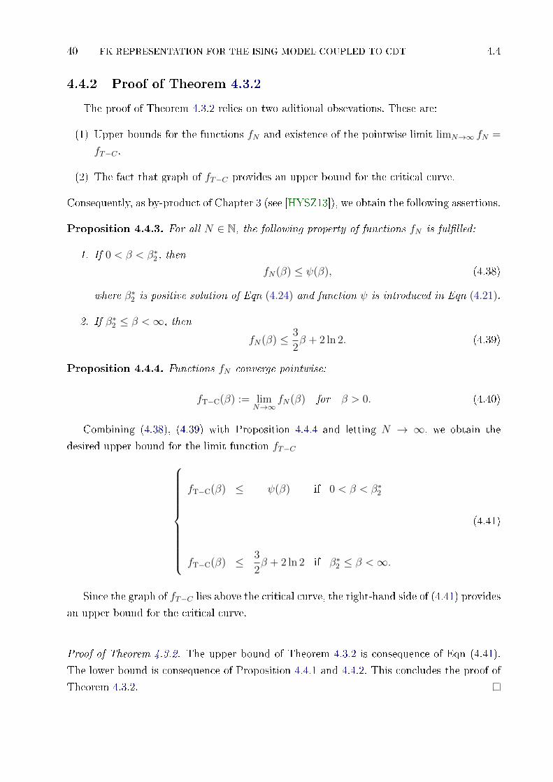
40 FK REPRESENTATION FOR THE ISING MODEL COUPLED TO CDT 4.4
4.4.2 Proof of Theorem 4.3.2
The proof of Theorem 4.3.2 relies on two aditional obsevations. These are:
(1) Upper bounds for the functions fN and existence of the pointwise limit limN→∞ fN =
fT−C .
(2) The fact that graph of fT−C provides an upper bound for the critical curve.
Consequently, as by-product of Chapter 3 (see [HYSZ13]), we obtain the following assertions.
Proposition 4.4.3. For all N ∈ N, the following property of functions fN is fullled:
1. If 0 < β < β∗2 , then
fN(β) ≤ ψ(β), (4.38)
where β∗2 is positive solution of Eqn (4.24) and function ψ is introduced in Eqn (4.21).
2. If β∗2 ≤ β <∞, then
fN(β) ≤ 3
2β + 2 ln 2. (4.39)
Proposition 4.4.4. Functions fN converge pointwise:
fT−C(β) := limN→∞
fN(β) for β > 0. (4.40)
Combining (4.38), (4.39) with Proposition 4.4.4 and letting N → ∞, we obtain the
desired upper bound for the limit function fT−C
fT−C(β) ≤ ψ(β) if 0 < β < β∗2
fT−C(β) ≤ 3
2β + 2 ln 2 if β∗2 ≤ β <∞.
(4.41)
Since the graph of fT−C lies above the critical curve, the right-hand side of (4.41) provides
an upper bound for the critical curve.
Proof of Theorem 4.3.2. The upper bound of Theorem 4.3.2 is consequence of Eqn (4.41).
The lower bound is consequence of Proposition 4.4.1 and 4.4.2. This concludes the proof of
Theorem 4.3.2.

Chapter 5
Potts model coupled to CDTs and FK
representation
In this chapter using a natural generalization of Ising model, we extend results from
before chapters for the (annealed) classical Ising model coupled to two-dimensional causal
dynamical triangulations. Such generalization is called of Potts model. Whereas in Ising sys-
tems the spins on two dierent values, in the q-state Potts model q distinct values, represent
by the elements of the set 1, . . . , q, are allowed on any vertex from the triangulation t.
In Chapter 3 and 4, the Ising model was dened putting spins on any triangles (faces), but
it is equivalent to put spins on any vertex of dual triangulation, dened in Section 5.2.2. Using
duality relation on a torus (periodic boundary condition), we provide a relation between the
free energy of Potts model coupled to CDTs and Potts model coupled to DUAL CDTs.
Additionally, using the high temperature expansion (and duality relation), we determined a
region where the critical curve can be located. This bound serves for Ising model case, and
improves the bounds found in the before chapters (Chapter 3: Theorem 4.3.1 and Theorem
4.3.2. Chapter 4: Lemma 3.2.1 and Theorem 3.2.2).
5.1 Introduction and main results of this chapter
A causal dynamical triangulation (CDT), introduced by Ambjørn and Loll (see [AL98]),
together with its predecessor a dynamical triangulation (DT), constitute attemps to provide
a meaning to formal expressions appearing in the path integral quantisation of gravity (see
[ADJ97], [AJ06] for an overview). The idea is to regularise the path integral by approximat-
ing the geometries emerging in the integration by CDTs. As a result, the path integral over
geometries is replaced with a sum over all possible triangulations where each conguration
is weighted by a Boltzmann factor e−µ|T |, with |T | standing for the size of the triangula-
tion and µ being the cosmological constant. The evaluation of the partition function was
reduced to a purely combinatorial problem that can be solved with the help of the early
work of Tutte [Tut62, Tut63]; alternatively, more powerful techniques were proposed, based
41

42 POTTS MODEL COUPLED TO CDTS AND FK REPRESENTATION 5.1
on random matrix models (see, e.g., [FGZJ95]) and bijections to well-labelled trees (see
[Sch97, BDG02]).
From a physical point of view it is interesting to study various models of matter, such as
the q-state Potts model, coupled to the CDT. The goal of this chapter is dene the q-state
Potts model coupled to CDTs and will use the FK representation for study this model. In this
case, the calculation of the partition function also reduces to a combinatorial problem. For
the 2-state Potts model (Ising model) coupled to a CDT some progress has been recently
made on existence of Gibbs measures and phase transitions (see [AAL99], [BL07], [HYSZ13]
and [Her14] for details). In particular, using transfer matrix methods, the Krein-Rutman
theory and FK representation for the Ising model, [Her14] provides a region in the quadrant
of parameters β, µ > 0 where the innite-volume free energy has a limit, providing results
on convergence and asymptotic properties of the partition function and the Gibbs measure.
Thus, FK-Potts models, introduced by Fortuin and Kasteleyn (see [FK72]), prove that these
models have become an important tool in the study of phase transition for the Ising and
q-state Potts model.
In general, the FK-Potts model on a nite connected graph (not necessarily planar) is
a model of edges of the graphs, each edge is either closed or open. The probability of a
conguration is proportional to
p#open edges(1− p)#closed edgesq#clusters
,
where the edge-weight p ∈ [0, 1] and the cluster-weight q ∈ (0,∞) are the parameters of the
model. For q ≥ 1, this model can be extended to innite-volume where it exhibits a phase
transition at some critical parameter pc(q), that depend on the geometry of the graph. In the
case of planar graphs, there is a connection between FK-Potts models on a graph and on its
dual with the same cluster-weight q and appropriately related edge-weight p and p∗ = p∗(p)
(Kramers-Wannier duality). For example, this relation leads in the particular case of Z2 to
a natural conjecture: the critical point is the same as the so-called self-dual point satisfying
psd = p∗(psd), proved by Beara and Duminil-Copin in [BC12].
In the case of a FK-Potts model dened on a causal dynamical triangulation t with pe-
riodic boundary condition, or equivalently dened on a torus (see Figure 3.1 for a geometric
representation), its dual, dened on t∗, is not a FK-Potts model; but will enough for our
purposes. This relation together with the Edwars-Sokal coupling, using p = 1− e−β, permits
nd a relation between the parameters (β, µ) of the Potts model coupled to CDT and the
parameters (β∗, µ∗) of its dual for the innite-volume (thermodynamic limit).
In the present chapter, we prove the following duality relation.
Theorem 5.1.1. Let q ≥ 2. The free energy of the q-state Potts model coupled to causal
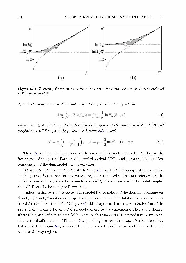
5.1 INTRODUCTION AND MAIN RESULTS OF THIS CHAPTER 43
(a) (b)
Figure 5.1: Illustrating the region where the critical curve for Potts model coupled CDTs and dual
CDTs can be located.
dynamical triangulation and its dual satised the following duality relation
limN→∞
1
Nln ΞN(β, µ) = lim
N→∞
1
Nln Ξ∗N(β∗, µ∗) (5.1)
where ΞN , Ξ∗N denote the partition function of the q-state Potts model coupled to CDT and
coupled dual CDT respectively (dened in Section 5.2.1), and
β∗ = ln
(1 +
q
eβ − 1
), µ∗ = µ− 3
2ln(eβ − 1) + ln q. (5.2)
Thus, (5.1) relates the free energy of the q-state Potts model coupled to CDTs and the
free energy of the q-state Potts model coupled to dual CDTs, and maps the high and low
temperature of the dual models onto each other.
We will use the duality relation of Theorem 5.1.1 and the high-temperature expansion
for the q-state Potts model for determine a region in the quadrant of parameters where the
critical curve for the q-state Potts model coupled CDTs and q-state Potts model coupled
dual CDTs can be located (see Figure 5.1).
Understanding by critical curve of the model the boundary of the domain of parameters
β and µ (β∗ and µ∗ on its dual, respectively) where the model exhibits subcritical behavior
(see denition in Section 4.3 of Chapter 4), this chapter makes a rigorous derivation of the
subcriticality domain for an q-Potts model coupled to two-dimensional CDT and a domain
where the tipical innite-volume Gibbs measure there no exists. The proof involve two tech-
niques: the duality relation (Theorem 5.1.1) and high-temperature expansion for the q-state
Potts model. In Figure 5.1, we show the region where the critical curve of the model should
be located (gray region).
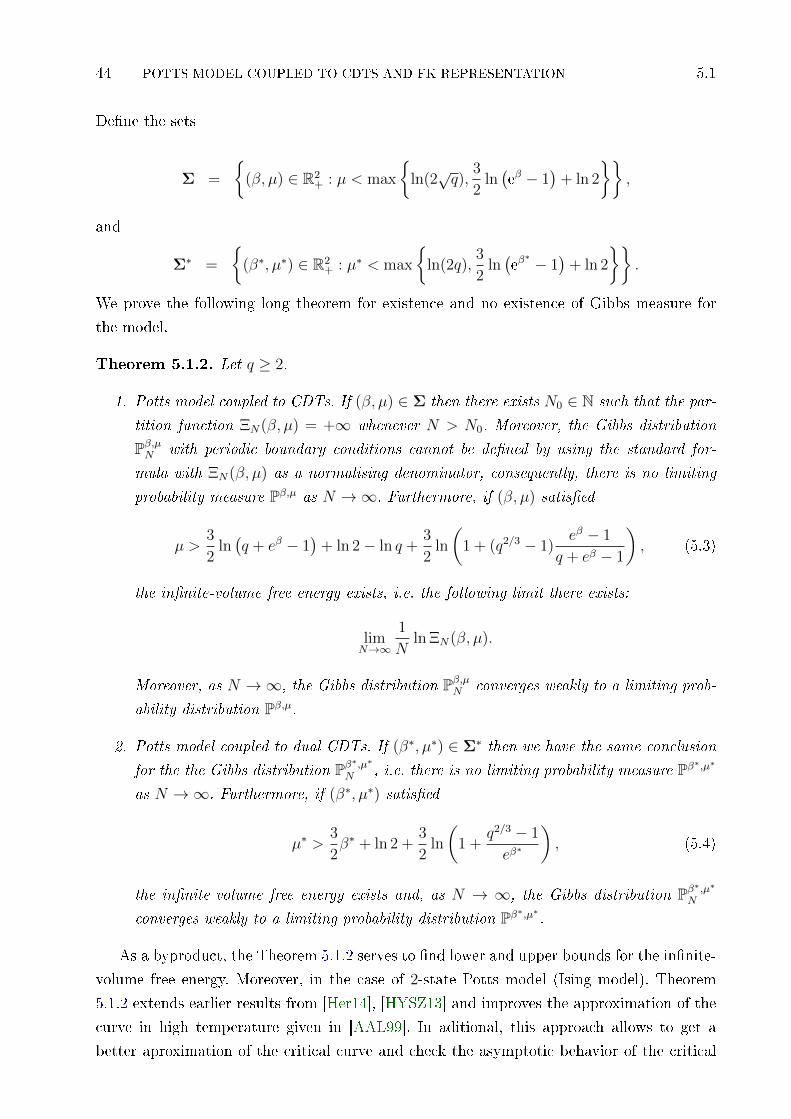
44 POTTS MODEL COUPLED TO CDTS AND FK REPRESENTATION 5.1
Dene the sets
Σ =
(β, µ) ∈ R2
+ : µ < max
ln(2√q),
3
2ln(eβ − 1
)+ ln 2
,
and
Σ∗ =
(β∗, µ∗) ∈ R2
+ : µ∗ < max
ln(2q),
3
2ln(eβ∗ − 1
)+ ln 2
.
We prove the following long theorem for existence and no existence of Gibbs measure for
the model.
Theorem 5.1.2. Let q ≥ 2.
1. Potts model coupled to CDTs. If (β, µ) ∈ Σ then there exists N0 ∈ N such that the par-
tition function ΞN(β, µ) = +∞ whenever N > N0. Moreover, the Gibbs distribution
Pβ,µN with periodic boundary conditions cannot be dened by using the standard for-
mula with ΞN(β, µ) as a normalising denominator, consequently, there is no limiting
probability measure Pβ,µ as N →∞. Furthermore, if (β, µ) satised
µ >3
2ln(q + eβ − 1
)+ ln 2− ln q +
3
2ln
(1 + (q2/3 − 1)
eβ − 1
q + eβ − 1
), (5.3)
the innite-volume free energy exists, i.e. the following limit there exists:
limN→∞
1
Nln ΞN(β, µ).
Moreover, as N →∞, the Gibbs distribution Pβ,µN converges weakly to a limiting prob-
ability distribution Pβ,µ.
2. Potts model coupled to dual CDTs. If (β∗, µ∗) ∈ Σ∗ then we have the same conclusion
for the the Gibbs distribution Pβ∗,µ∗
N , i.e. there is no limiting probability measure Pβ∗,µ∗
as N →∞. Furthermore, if (β∗, µ∗) satised
µ∗ >3
2β∗ + ln 2 +
3
2ln
(1 +
q2/3 − 1
eβ∗
), (5.4)
the innite-volume free energy exists and, as N → ∞, the Gibbs distribution Pβ∗,µ∗
N
converges weakly to a limiting probability distribution Pβ∗,µ∗.
As a byproduct, the Theorem 5.1.2 serves to nd lower and upper bounds for the innite-
volume free energy. Moreover, in the case of 2-state Potts model (Ising model), Theorem
5.1.2 extends earlier results from [Her14], [HYSZ13] and improves the approximation of the
curve in high temperature given in [AAL99]. In aditional, this approach allows to get a
better aproximation of the critical curve and check the asymptotic behavior of the critical

5.2 NOTATIONS 45
curve given in [AAL99], and it say that critical curve is asymptotic to 32β + ln 2, for q ≥ 2.
In Theorem 5.1.2, we nd a lower and upper curve that converges fast to 32β + ln 2.
5.2 Notations
In this section we rts introduce notations and give a summary of q-state Potts model and
we dene the Potts model coupled to CDTs. Finally, we give a short review of the Edwards-
Sokal coupling. We refer to [MYZ01], [Gri06], [HYSZ13], for more details. We attempt at
establishing regions where the innite-volume free energy converges, yielding results on the
convergence and asymptotic properties of the partition function and the Gibbs measure.
5.2.1 A Potts model coupled to CDTs
Let t be a CDT on the cylinder CN with periodic boundary condition. Each triangulation
t can be view as a graph t = (V (t), E(t)) embedded on a torus. Potts spin systems are
generalizations of the Ising model. Whereas in Ising systems the spins on two dierent
values, in the q-state Potts model q distinct values, represent by the elements of the set
1, . . . , q, are allowed on any vertex from the triangulation t. We consider the product
sample space Ω(t) = 1, . . . , qV (t) and we consider a usual (ferromagnetic) q-state Potts
model energy, where two spins σ(t) and σ(t′) interact if their supporting vertices t, t′ are
connected by an common edge; such vertices are called nearest neighbors, and this property
is reected in the notation 〈t, t′〉. Thus, the Hamiltonian used for the q-state Potts model
on t is given by
h(σ) = −∑〈t,t′〉
δσ(t),σ(t′). (5.5)
The partition function for the q-state Potts model on t is dene by
ZP (β, q, t) =∑σ
exp−βh(σ)
, (5.6)
where the summation is over any congurations σ ∈ 1, . . . , qV (t). Thus, the q-state Potts
measure on t is dene as follows
µtβ,q(σ) =
1
ZP (β, q, t)exp−βh(σ)
. (5.7)
Using the partition function for the q-state Potts model on a xed t, we dene the partition
function for the q-state Potts model coupled to CDTs, at the inverse temperature β > 0 and
the cosmological constant µ, as follows
ΞN(β, µ) =∑t
exp−µn(t)
ZP (β, q, t) (5.8)
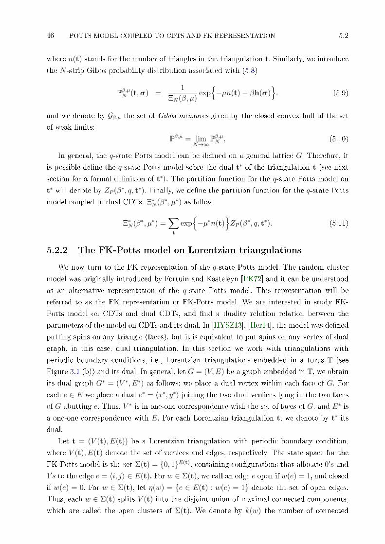
46 POTTS MODEL COUPLED TO CDTS AND FK REPRESENTATION 5.2
where n(t) stands for the number of triangles in the triangulation t. Similarly, we introduce
the N -strip Gibbs probability distribution associated with (5.8)
Pβ,µN (t,σ) =1
ΞN(β, µ)exp−µn(t)− βh(σ)
. (5.9)
and we denote by Gβ,µ the set of Gibbs measures given by the closed convex hull of the set
of weak limits:
Pβ,µ = limN→∞
Pβ,µN , (5.10)
In general, the q-state Potts model can be dened on a general lattice G. Therefore, it
is possible dene the q-state Potts model sobre the dual t∗ of the triangulation t (see next
section for a formal denition of t∗). The partition function for the q-state Potts model on
t∗ will denote by ZP (β∗, q, t∗). Finally, we dene the partition function for the q-state Potts
model coupled to dual CDTs, Ξ∗N(β∗, µ∗) as follow
Ξ∗N(β∗, µ∗) =∑t
exp−µ∗n(t)
ZP (β∗, q, t∗). (5.11)
5.2.2 The FK-Potts model on Lorentzian triangulations
We now turn to the FK representation of the q-state Potts model. The random cluster
model was originally introduced by Fortuin and Kasteleyn [FK72] and it can be understood
as an alternative representation of the q-state Potts model. This representation will be
referred to as the FK representation or FK-Potts model. We are interested in study FK-
Potts model on CDTs and dual CDTs, and nd a duality relation relation between the
parameters of the model on CDTs and its dual. In [HYSZ13], [Her14], the model was dened
putting spins on any triangle (faces), but it is equivalent to put spins on any vertex of dual
graph, in this case, dual triangulation. In this section we work with triangulations with
periodic boundary conditions, i.e., Lorentzian triangulations embedded in a torus T (see
Figure 3.1 (b)) and its dual. In general, let G = (V,E) be a graph embedded in T, we obtainits dual graph G∗ = (V ∗, E∗) as follows: we place a dual vertex within each face of G. For
each e ∈ E we place a dual e∗ = 〈x∗, y∗〉 joining the two dual vertices lying in the two faces
of G abutting e. Thus, V ∗ is in one-one correspondence with the set of faces of G, and E∗ is
a one-one correspondence with E. For each Lorentzian triangulation t, we denote by t∗ its
dual.
Let t = (V (t), E(t)) be a Lorentzian triangulation with periodic boundary condition,
where V (t), E(t) denote the set of vertices and edges, respectively. The state space for the
FK-Potts model is the set Σ(t) = 0, 1E(t), containing congurations that allocate 0′s and
1′s to the edge e = 〈i, j〉 ∈ E(t). For w ∈ Σ(t), we call an edge e open if w(e) = 1, and closed
if w(e) = 0. For w ∈ Σ(t), let η(w) = e ∈ E(t) : w(e) = 1 denote the set of open edges.
Thus, each w ∈ Σ(t) splits V (t) into the disjoint union of maximal connected components,
which are called the open clusters of Σ(t). We denote by k(w) the number of connected

5.2 NOTATIONS 47
Figure 5.2: Geometric representation of a dual Lorentzian triangulation t∗ with periodic spatial
boundary condition.
components (open clusters) of the graph (V (t), η(w)), and note that k(w) includes a count
of isolated vertices. Two sites of t are said to be connected if one can be reached from another
via a chain of open bonds.
The partition function of the FK-Potts model on t with parameters p and q and periodic
boundary condition is dened by
ZFK(p, q, t) =∑
w∈Σ(t)
∏e∈E(t)
(1− p)1−w(e)pw(e)
qk(w), (5.12)
Thus, the FK-Potts measure on t is dene as follows
Φtp,q(w) =
1
ZFK(p, q, t)
∏e∈E(t)
(1− p)1−w(e)pw(e)
qk(w). (5.13)
We will use a similarly notation for the FK-Potts model on dual triangulation t∗. We
denote by ZFK(p∗, q, t∗) and Φt∗p∗,q the partition function and the FK-Potts measure on t∗
with parameters p∗ and q, respectively.
5.2.3 The relation between the Potts model and FK-Potts model:
Edwards-Sokal coupling
There are several ways to make the connection between the Potts and FK-Potts model.
The correspondence between the q-state Potts model and FK-Potts model was established
by Fortuin and Kasteleyn [FK72] (see also [ES88], [Gri06]). In a modern approach, these two
models are related via a coupling, i.e., coupled the two systems on a common probability
space. This coupling was introduced by Edwards-Sokal in [ES88].
Let t be a CDT on the cylinder CN with periodic boundary condition. We consider the

48 POTTS MODEL COUPLED TO CDTS AND FK REPRESENTATION 5.2
product sample space Ω(t)×Σ(t) where Ω(t) = 1, 2, . . . , qV (t) and Σ(t) = 0, 1E(t). The
Edwards-Sokal measure Q on Ω(t)× Σ(t) is dene by
Q(σ,w) ∝∏
e=i,j∈E(t)
(1− p)δw(e),0 + pδw(e),1δσi,σj
Theorem 5.2.1 (Edwards-Sokal [ES88]). Let q ∈ 2, 3, . . . . Let p ∈ (0, 1) and t a CDT with
periodic boundary condition, and suppose that p = 1−e−β. If the conguration w is distributed
according to an FK-Potts measure with parameters (p, q) on t, then σ is distributed according
to a q-state Potts measure with inverse temperature β. Furthermore, the Edwards-Sokal
measure provides a coupling of µtβ,q and Φt
p,q, i.e.∑w∈Σ(t)
Q(σ,w) = µtβ,q(σ),
for all σ ∈ Ω(t), and ∑σ∈Ω(t)
Q(σ,w) = Φtp,q(w),
for all w ∈ Σ(t). Moreover, we have the relation between partition functions
ZFK(p, q, t) = e−β|E(t)|ZP (β, q, t). (5.14)
5.2.4 Duality for FK-Potts model coupled to CDTs with periodic
boundary conditions
In this section we obtain a relation between the partition functions of FK-Potts model
on a triangulation t and its dual. This relation was studied by Beara and Duminil-Copin
for the FK-Potts model on Z2 with free, wired and periodic boundary condition (see [BC12]
for details). We will view wich the dual of a FK-Potts model dened on a torus is a quasi
FK-Potts model, but it is not very dierent from one.
Let t and t∗ a CDT with periodic boundary condition and its dual. Each conguration
w ∈ Σ(t) = 0, 1E(t) gives rise to a dual conguration w∗ ∈ Σ(t∗) = 0, 1E(t∗) given by
w∗(e∗) = 1 − w(e). That is, e∗ is declared open if and only if the corresponding bond e is
closed. The new conguration w∗ is called the dual conguration of w, and note that there
exists an one-one correspondence between Σ(t) and Σ(t∗). As in the Section 5.2.2, to each
conguration w∗ there corresponds the set η(w∗) = e∗ ∈ E(t∗) : w∗(e∗) = 1 of its openedges.
Now, beginning of FK-Potts model on t, we try to obtain the dual model on the dual
triangulation t∗.
Let o(w) (resp. c(w)) denote the number of open edges (resp. closed) of w, k(w) the
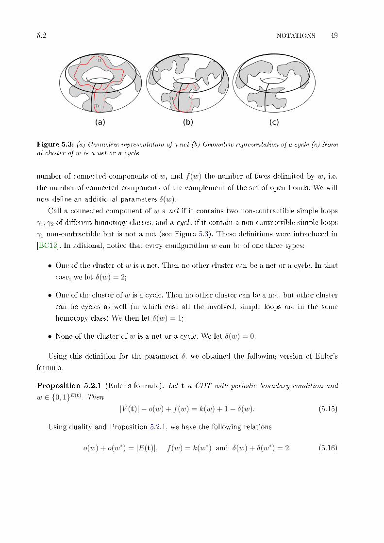
5.2 NOTATIONS 49
(a) (b) (c)
Figure 5.3: (a) Geometric representation of a net (b) Geometric representation of a cycle (c) None
of cluster of w is a net or a cycle
number of connected components of w, and f(w) the number of faces delimited by w, i.e.
the number of connected components of the complement of the set of open bonds. We will
now dene an additional parameters δ(w).
Call a connected component of w a net if it contains two non-contractible simple loops
γ1, γ2 of dierent homotopy classes, and a cycle if it contain a non-contractible simple loops
γ1 non-contractible but is not a net (see Figure 5.3). These denitions were introduced in
[BC12]. In aditional, notice that every conguration w can be of one three types:
• One of the cluster of w is a net. Then no other cluster can be a net or a cycle. In that
case, we let δ(w) = 2;
• One of the cluster of w is a cycle. Then no other cluster can be a net, but other cluster
can be cycles as well (in which case all the involved, simple loops are in the same
homotopy class) We then let δ(w) = 1;
• None of the cluster of w is a net or a cycle. We let δ(w) = 0.
Using this denition for the parameter δ, we obtained the following version of Euler's
formula.
Proposition 5.2.1 (Euler's formula). Let t a CDT with periodic boundary condition and
w ∈ 0, 1E(t). Then
|V (t)| − o(w) + f(w) = k(w) + 1− δ(w). (5.15)
Using duality and Proposition 5.2.1, we have the following relations
o(w) + o(w∗) = |E(t)|, f(w) = k(w∗) and δ(w) + δ(w∗) = 2. (5.16)
50 POTTS MODEL COUPLED TO CDTS AND FK REPRESENTATION 5.2
Let q ∈ (0,∞) and p ∈ (0, 1). The partition function of the FK-Potts model is given by
ZFK(p, q, t) =∑
w∈Σ(t)
∏e∈E(t)
(1− p)1−w(e)pw(e)
qk(w)
=∑
w∈Σ(t)
po(w)(1− p)c(w)qk(w).
Using Euler's formula and relations (5.16), we rewrite the number of cluster of w in terms
of its dual w∗
k(w) = |V (t)| − |E(t)|+ o(w∗) + k(w∗) + 1− δ(w∗).
We note also that o(w) + o(w∗) = |E(t)| = |E(t∗)|. Plugging before relations into the
partition function of the FK-Potts model, we obtain
ZFK(p, q, t) =∑
w∈Σ(t)
po(w)(1− p)|E(t)|−o(w)qk(w)
= (1− p)|E(t)|∑
w∈Σ(t)
(p
1− p
)o(w)
qk(w)
= (1− p)|E(t)|∑
w∈Σ(t)
(p
1− p
)|E(t)|−o(w∗)
q|V (t)|−|E(t)|+o(w∗)+k(w∗)+1−δ(w∗)
= p|E(t)|q|V (t)|−|E(t)|∑
w∈Σ(t)
(1− pp
)o(w∗)qo(w
∗)+k(w∗)+1−δ(w∗)
As there exists an one-one correspondence between Σ(t) and Σ(t∗), in the last equality, we
we change the sum in Σ(t) by the sum in Σ(t∗). Thus, we obtain the following representation
of the partition function in terms of the dual triangulation and dual congurations
ZFK(p, q, t) = p|E(t)|q|V (t)|−|E(t)|∑
w∗∈Σ(t∗)
(q(1− p)
p
)o(w∗)qk(w∗)+1−δ(w∗) (5.17)
Using the relation (5.17), we obtain the following lemma.
Lemma 5.2.1. Let t be a CDT with periodic boundary condition. Then the following com-
parison inequalities both
ZFK(p, q, t) ≤(
p
1− p∗
)|E(t)|
q|V (t)|−|E(t)|+1ZFK(p∗, q, t∗) (5.18)

5.2 NOTATIONS 51
and (p
1− p∗
)|E(t)|
q|V (t)|−|E(t)|−1ZFK(p∗, q, t∗) ≤ ZFK(p, q, t) (5.19)
where ZFK(p∗, q, t∗) is the partition function for FK-Potts model on t∗ with parameters q
and p∗ = p∗(p, q) satisfying
p∗(p, q) =(1− p)q
(1− p)q + p, or equivalently
p∗
1− p∗· p
1− p= q.
Proof. We introduce the parameter p∗ = p∗(p, q) as solution of the equation
p∗
1− p∗=
(1− p)qp
.
Thus, the partition function can be written in the following ways
ZFK(p, q, t) = p|E(t)|q|V (t)|−|E(t)|∑
w∗∈Σ(t∗)
(p∗
1− p∗
)o(w∗)qk(w∗)+1−δ(w∗)
=p|E(t)|
(1− p∗)|E(t∗)| q|V (t)|−|E(t)|(1− p∗)|E(t∗)|
∑w∗∈Σ(t∗)
(p∗
1− p∗
)o(w∗)qk(w∗)+1−δ(w∗).
Notice that −1 ≤ 1 − δ(w∗) ≤ 1, for all w∗ ∈ Σ(t∗). We dene ZFK(p∗, q, t∗), the partition
function of a FK-Potts model with parameters p∗ and q. Thus, we obtain the upper bound
ZFK(p, q, t) ≤ p|E(t)|
(1− p∗)|E(t∗)| q|V (t)|−|E(t)|+1ZFK(p∗, q, t∗) ,
and the lower bound
p|E(t)|
(1− p∗)|E(t∗)| q|V (t)|−|E(t)|−1ZFK(p∗, q, t∗) ≤ ZFK(p, q, t)
for the partition function of FK-Potts model on t with parameters p and q. Using the one-one
correspondence between E(t) and E(t∗), we conclude the proof.
The partition function for pure CDT's has been determined as a sum over all possible
triangulations of a cylinder where each conguration is weighted by a Boltzmann factor
e−µn(t), where n(t) standing for the size of the triangulation and µ being the cosmological
constant. Thus, in quantum gravity the volume n(t) becomes a dynamical variable for the
model. Therefore, we rewrite the duality relation ( Lemma 5.2.1) for the partition function
of the FK-Potts model on a triangulation t, in terms of dynamical variable n(t). In the Table
5.1 we show the relation among V (t), E(t), V (t∗), E(t∗) and the number of triangles n(t) of
a CDT t.
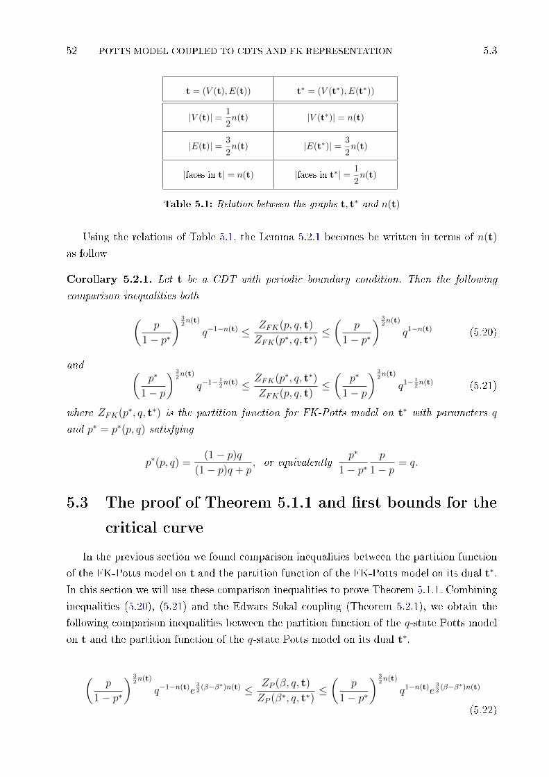
52 POTTS MODEL COUPLED TO CDTS AND FK REPRESENTATION 5.3
t = (V (t), E(t)) t∗ = (V (t∗), E(t∗))
|V (t)| = 1
2n(t) |V (t∗)| = n(t)
|E(t)| = 3
2n(t) |E(t∗)| = 3
2n(t)
|faces in t| = n(t) |faces in t∗| = 1
2n(t)
Table 5.1: Relation between the graphs t, t∗ and n(t)
Using the relations of Table 5.1, the Lemma 5.2.1 becomes be written in terms of n(t)
as follow
Corollary 5.2.1. Let t be a CDT with periodic boundary condition. Then the following
comparison inequalities both
(p
1− p∗
) 32n(t)
q−1−n(t) ≤ ZFK(p, q, t)
ZFK(p∗, q, t∗)≤(
p
1− p∗
) 32n(t)
q1−n(t) (5.20)
and (p∗
1− p
) 32n(t)
q−1− 12n(t) ≤ ZFK(p∗, q, t∗)
ZFK(p, q, t)≤(
p∗
1− p
) 32n(t)
q1− 12n(t) (5.21)
where ZFK(p∗, q, t∗) is the partition function for FK-Potts model on t∗ with parameters q
and p∗ = p∗(p, q) satisfying
p∗(p, q) =(1− p)q
(1− p)q + p, or equivalently
p∗
1− p∗p
1− p= q.
5.3 The proof of Theorem 5.1.1 and rst bounds for the
critical curve
In the previous section we found comparison inequalities between the partition function
of the FK-Potts model on t and the partition function of the FK-Potts model on its dual t∗.
In this section we will use these comparison inequalities to prove Theorem 5.1.1. Combining
inequalities (5.20), (5.21) and the Edwars Sokal coupling (Theorem 5.2.1), we obtain the
following comparison inequalities between the partition function of the q-state Potts model
on t and the partition function of the q-state Potts model on its dual t∗.
(p
1− p∗
) 32n(t)
q−1−n(t)e32
(β−β∗)n(t) ≤ ZP (β, q, t)
ZP (β∗, q, t∗)≤(
p
1− p∗
) 32n(t)
q1−n(t)e32
(β−β∗)n(t)
(5.22)

5.3 THE PROOF OF THEOREM 5.1.1 AND FIRST BOUNDS FOR THE CRITICAL CURVE 53
and(p∗
1− p
) 32n(t)
q−1− 12n(t)e
32
(β∗−β)n(t) ≤ ZP (β∗, q, t∗)
ZP (β, q, t)≤(
p∗
1− p
) 32n(t)
q1− 12n(t)e
32
(β∗−β)n(t)
(5.23)
where (eβ − 1)(eβ∗ − 1) = q.
Proof of Theorem 5.1.1. Using the comparison inequalities (5.22) and (5.23), we will nd
comparison inequalities for the partition functions of the Potts model coupled CDTs with
parameters β, µ and dual CDTs with parameters β∗ = β∗(β), µ∗ = µ∗(β, µ). Remember that
p∗ = 1− e−β∗ and p = 1− e−β. Thus,
p∗
1− p= (1− e−β∗) + qe−β
∗=
q
(1− e−β) + qe−β
andp
1− p∗=
q
(1− e−β∗) + qe−β∗= (1− e−β) + qe−β.
Multiplying by the Boltzmann factor e−µn(t) in (5.22) and (5.23), and sum over all possible
CDTs of the cylinder CN , we obtain the following comparison inequalities
1
qΞ∗N(β∗, µ∗) ≤ ΞN(β, µ) ≤ qΞ∗N(β∗, µ∗) (5.24)
where Ξ∗N stands the partition function of the q-state Potts model coupled to dual CDTs
with periodic boundary condition, ΞN stands the partition function of the q-state Potts
model coupled to CDTs with periodic boundary condition, and
β∗ = ln
(1 +
q
eβ − 1
), µ∗ = µ− 3
2ln(eβ − 1) + ln q.
Similarly, we have1
qΞN(β, µ) ≤ Ξ∗N(β∗, µ∗) ≤ qΞN(β, µ) (5.25)
where
β = ln
(1 +
q
eβ∗ − 1
), µ = µ∗ − 3
2ln(eβ
∗ − 1) +1
2ln q.
Take the natural logarithm in inequalities (5.24) and (5.25), divide both sides of the above
inequalities by N and let N →∞. This concludes the proof of Theorem 5.1.1.
Theorem 5.1.1 provide an interesting reformulation in terms of free energy of the q-state
Potts model coupled to CDTs and its dual. This theorem relates the free energy of the q-
state Potts model coupled CDTs and the free energy of the q-state Potts model coupled dual
CDTs, and maps the high and low temperature of the dual models onto each other.
54 POTTS MODEL COUPLED TO CDTS AND FK REPRESENTATION 5.3
Using Edwars-Sokal coupling for the partition functions (5.14), duality relation found in
Theorem 5.1.1 and asymptotic properties (2.14), (3.20) of the partition function for pure
CDTs (see [MYZ01] for more details), we will obtain the rst bounds for the critical curve
of the q-state Potts model coupled to CDTs and dual CDTs. Let t be a CDT with periodic
boundary condition. We dene the set Πi of congurations in Σ(t) which splits V (t) in i
maximal connected components, i.e.
Πi = w ∈ Σ(t) : k(w) = i.
Similarly, we denote Π∗i the set of congurations in Σ(t∗) which splits V (t∗) in i maximal
connected components. Thus, we have the following representation for the partition function
of q-state Potts model on t
ZP (β, q, t) = eβ|E(t)|φtp(q
k(w)) = eβ|E(t)||V (t)|∑i=1
qiφtp(Πi), (5.26)
and on t∗
ZP (β∗, q, t∗) = eβ|E(t∗)|φt∗
p (qk(w∗)) = eβ|E(t∗)||V (t∗)|∑i=1
qiφt∗
p∗(Π∗i ), (5.27)
where φtp, φ
t∗p∗ denotes product measures on Σ(t) and Σ(t∗), respectively.
Using Table 5.1, we write the representations (5.26), (5.27) for the partition function in
terms of the dynamical variable n(t). For that, we consider two cases of interest separately.
1. The model on CDTs t: In this case, we can to write the partition function in terms of
volume n(t) of the triangulation as follow
ZP (β, q, t) = e32βn(t)
12n(t)∑i=1
qiφtp(Πi). (5.28)
Using the rst and latter term on the right-hand side of (5.28), we obtain two lower bounds
for the partition function of the Potts model on t
ZP (β, q, t) ≥ q(eβ − 1
) 32n(t)
, ZP (β, q, t) ≥ q12n(t). (5.29)
These lower bounds for the q-state Potts model on t permit to obtain a lower barrier for
parameters where the model can be dened, and the partition function of the model coupled
to CDTs could no explode in nite volume. These lower bounds serves to obtain information
of the Gibbs measure for q-state Potts model coupled to CDTs.

5.3 THE PROOF OF THEOREM 5.1.1 AND FIRST BOUNDS FOR THE CRITICAL CURVE 55
Proposition 5.3.1. If (β, µ) ∈ R+ such that
µ <1
2ln q + ln 2 or µ <
3
2ln(eβ − 1) + ln 2,
then there exists N0 ∈ N such that the partition function ΞN(β, µ) = ∞ whenever N >
N0. Moreover, the Gibbs distribution Pβ,µN cannot be dened by using the standard formula
with ΞN(β, µ) as a normalising denominator, consequently, there is no limiting probability
measure Pβ,µ as N →∞.
Proof. The lower bounds in (5.29) to ZP (β, q, t) provide the following lower bounds to
ΞN(β, µ),
ΞN(β, µ) ≥ q∑t
e−µ−32
ln(eβ−1)n(t), ΞN(β, µ) ≥ q∑t
e−µ−12
ln qn(t). (5.30)
Using asymptotic properties of Proposition (2.2.1), we obtain which the partition function
ΞN(β, µ) there is no exist if
µ ≤ 1
2ln q + ln
(2 cos
π
N + 1
)or µ ≤ 3
2ln(eβ − 1) + ln
(2 cos
π
N + 1
).
Letting N →∞, we conclude the proof.
Now, notice that12n(t)∑i=1
qiφtp(Πi) ≤ q
12n(t),
for any triangulation t. Thus, we obtain a upper bound for the partition function of the
q-state Potts model on t,
ZP (β, q, t) ≤ e32βn(t)q
12n(t) = e(
32β+ 1
2ln q)n(t). (5.31)
This upper bound for the q-state Potts model on t, permit to obtain a rst upper barrier
for the critical curve of the q-state Potts model coupled to CDTs, and above of that upper
bound the model exhibits subcritical behavior. Moreover, this upper bound for the critical
curve of the model coupled serves to obtain information of the Gibbs measure for the q-state
Potts model coupled to CDTs. We get the following result.
Proposition 5.3.2. Under condition µ >3
2β +
1
2ln q+ ln 2, the innite-volume free energy
exists, i.e. the following limit there exists:
limN→∞
1
Nln ΞN(β, µ).
Moreover, as N →∞, the Gibbs distribution Pβ,µN converges weakly to a limiting probability
distribution Pβ,µ.

56 POTTS MODEL COUPLED TO CDTS AND FK REPRESENTATION 5.3
Proof. Using inequality (5.31), we get to
ΞN(β, µ) ≤∑t
e−µ−32β− 1
2ln qn(t)
By Proposition 2.2.1, we obtain which the free energy there exists if µ− 32β − 1
2ln q > ln 2.
This concludes the proof.
Finally, using the duality relation (Theorem 5.1.1) and bounds found before propositions,
we obtain bounds for the critical curve for the q-state Potts model coupled to dual CDTs.
from CDTs tby duality−−−−−−−−→ to dual CDTs t∗
µ <1
2ln q + ln 2 → µ∗ <
3
2ln(eβ
∗− 1) + ln 2
µ <3
2ln(eβ − 1) + ln 2 → µ∗ < ln q + ln 2
µ >3
2β +
1
2ln q + ln 2 → µ∗ >
3
2ln(q + eβ
∗− 1) + ln 2
Table 5.2: Bounds for the critical curve of the q-state Potts model on CDTs will generate bounds
on its dual.
In Table 5.2 the parameters (β, µ) and (β∗, µ∗) satised the duality relation (5.2).
2. The model on dual CDTs t∗: Similarly, we write the partition function in terms of
volume n(t) of the triangulation as follow
ZP (β∗, q, t∗) = e32β∗n(t)
n(t)∑i=1
qiφt∗
p∗(Π∗i ). (5.32)
Using the rst and latter term on the right-hand side of (5.32), we obtain two lower bounds
for the partition function of the q-state Potts model on t∗
ZP (β∗, q, t∗) ≥ q(eβ∗ − 1
) 32n(t)
, ZP (β∗, q, t∗) ≥ qn(t), (5.33)
and an upper bound
ZP (β∗, q, t∗) ≤ e32β∗n(t)qn(t) = e(
32β∗+ln q)n(t). (5.34)
Using asymptotic properties of Theorem 2.2.1 and Proposition 2.2.1, bounds (5.33) and
(5.34) provide bounds for the critical curve of the q-state Potts model coupled dual CDTs.
As in before case, we have the following proposition to existence and non existence of Gibbs
measures of the model.
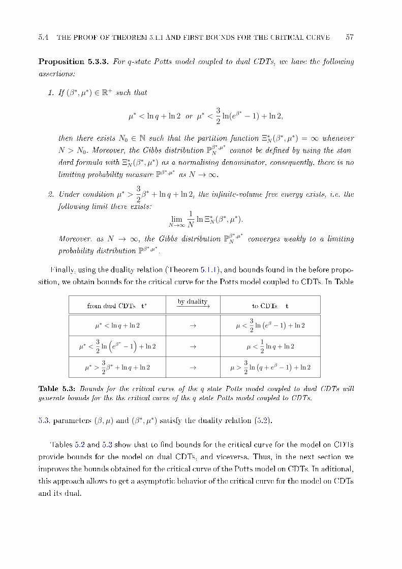
5.4 THE PROOF OF THEOREM 5.1.1 AND FIRST BOUNDS FOR THE CRITICAL CURVE 57
Proposition 5.3.3. For q-state Potts model coupled to dual CDTs, we have the following
assertions:
1. If (β∗, µ∗) ∈ R+ such that
µ∗ < ln q + ln 2 or µ∗ <3
2ln(eβ
∗ − 1) + ln 2,
then there exists N0 ∈ N such that the partition function Ξ∗N(β∗, µ∗) = ∞ whenever
N > N0. Moreover, the Gibbs distribution Pβ∗,µ∗
N cannot be dened by using the stan-
dard formula with Ξ∗N(β∗, µ∗) as a normalising denominator, consequently, there is no
limiting probability measure Pβ∗,µ∗ as N →∞.
2. Under condition µ∗ >3
2β∗ + ln q + ln 2, the innite-volume free energy exists, i.e. the
following limit there exists:
limN→∞
1
Nln Ξ∗N(β∗, µ∗).
Moreover, as N → ∞, the Gibbs distribution Pβ∗,µ∗
N converges weakly to a limiting
probability distribution Pβ∗,µ∗.
Finally, using the duality relation (Theorem 5.1.1), and bounds found in the before propo-
sition, we obtain bounds for the critical curve for the Potts model coupled to CDTs. In Table
from dual CDTs t∗by duality−−−−−−−−→ to CDTs t
µ∗ < ln q + ln 2 → µ <3
2ln(eβ − 1
)+ ln 2
µ∗ <3
2ln(eβ
∗− 1)+ ln 2 → µ <
1
2ln q + ln 2
µ∗ >3
2β∗ + ln q + ln 2 → µ >
3
2ln(q + eβ − 1
)+ ln 2
Table 5.3: Bounds for the critical curve of the q-state Potts model coupled to dual CDTs will
generate bounds for the the critical curve of the q-state Potts model coupled to CDTs.
5.3, parameters (β, µ) and (β∗, µ∗) satisfy the duality relation (5.2).
Tables 5.2 and 5.3 show that to nd bounds for the critical curve for the model on CDTs
provide bounds for the model on dual CDTs, and viceversa. Thus, in the next section we
improves the bounds obtained for the critical curve of the Potts model on CDTs. In aditional,
this approach allows to get a asymptotic behavior of the critical curve for the model on CDTs
and its dual.

58 POTTS MODEL COUPLED TO CDTS AND FK REPRESENTATION 5.4
5.4 High-T expansion of the Potts model and Proof of
Theorem 5.1.2
Let t be a CDT with periodic boundary condition. The partition function for the Potts
model on t is write in the usual high-T expansion as
ZP (β, q, t) =
(q + h
q
)|E(t)|∑σ
∏〈i,j〉
(1 + fij) (5.35)
where h = eβ − 1 and fij = hq+h
(−1 + qδσi,σj). It can be readily veried that∑
σ fij = 0 for
all i, j ∈ E(t), consequently, all subgraphs with one or more vertices of degree 1 give rise
to zero contributions. Thus, the partition function can be written as follow
ZP (β, q, t) =
(q + h
q
)|E(t)|∑σ
∑A∈G(t)
∏i,j∈A
fij,
where G(t) is the set of families of edges of t without vertices of degree 1. Therefore, we can
rewrite the partition function as
ZP (β, q, t) =
(q + h
q
)|E(t)| ∑A∈G(t)
w(A)
where w(A) =∑σ
∏i,j∈A
fij is a weight factor associated with the subset A. We then pro-
ceeded to determine w(A). An expression of w(A) for general A can be obtained by further
expanding in w(A) the product∑σ
∏i,j∈A
fij. This procedure leads to
w(A) =
(h
q + h
)|A|∑σ
P(A)(σ),
where P(A)(σ) =∏
e∈A(−1 + qδe(σ)), and if e = i, j then δe(σ) = δσi,σj . Expanding
P(A)(σ), we have the following representation
P(A)(σ) = (−1)|A| + (−1)|A|−1q∑e∈A
δe(σ) + (−1)|A|−2q2∑
e1,e2∈A
δe1(σ)δe2(σ)
+ · · ·+ (−1)q|A|−1∑
e1,...,e|A|−1∈A
δe1(σ) . . . δe|A|−1(σ)
+q|A|δe1(σ) . . . δe|A|(σ).

5.4 HIGH-T EXPANSION OF THE POTTS MODEL AND PROOF OF THEOREM 5.1.2 59
Figure 5.4: Examples of three subgraphs of A with 8 edges. It is clear that the term ξ(e1, . . . , e8)depends of the topology of the subgraphs.
We choose k edges e1, . . . , ek of A. These edges form a subgraph of A. Thus, we obtain∑σ
δe1(σ) . . . δek(σ) = q|V (t)|−k+ξ(e1,...,ek)
where ξ(e1, . . . , ek) stands the total numbers of internal faces in each maximal connected
component of e1, . . . , ek (number of independent circuits in e1, . . . , ek). Note that this
terms depends essentially on the topology of e1, . . . , ek (see Figure 5.4). But ξ(e1, . . . , ek) ≤2
3(k + 1) for all k. Thus, we obtain the estimate
∑σ
δe1(σ) . . . δek(σ) ≤ q|V (t)|−k+ 23
(k+1) = q|V (t)|− k3
+ 23
and ∑σ
∑e1,...ek∈A
δe1(σ) . . . δek(σ) ≤(|A|k
)q|V (t)|− k
3+ 2
3 .

60 POTTS MODEL COUPLED TO CDTS AND FK REPRESENTATION 5.4
Therefore,
∑σ
P(A)(σ) ≤ q|V (t)|+ 23
|A|∑k=0
(|A|k
)(−1)|A|−k( 3
√q2)k = q|V (t)|+ 2
3 ( 3√q2 − 1)|A|,
and
ZP (β, q, t) ≤(q + h
q
)|E(t)|
q|V (t)|+ 23
∑A∈G(t)
(( 3√q2 − 1)
h
q + h
)|A|
≤(q + h
q
)|E(t)|
q|V (t)|+ 23
(1 +
∑k≥1
Ωk(t)uk
),
where Ωk(t) = |A ∈ G(t) : |A| = k| and u = ( 3√q2 − 1)
h
q + h. But Ωk(t) ≤
(|E(t)|k
). Thus,
we get the estimate
ZP (β, q, t) ≤(q + h
q
)|E(t)|
q|V (t)|+ 23 (1 + u)|E(t)|. (5.36)
Proof of Theorem 5.1.2. Using estimate (5.36) and Table 5.1, we write the new bound (5.36)
for the partition function of the Potts model on t in terms of the dynamical variable n(t),
and make similarly computations for the dual case. For that, we consider two cases of interest
separately.
1. The model on CDTs t: In this case, we can to write the new bound for the partition
function in terms of volume n(t) of the triangulation as follow
ZP (β, q, t) ≤(q + h
q
) 32n(t)
q12n(t)+ 2
3 (1 + u)32n(t). (5.37)
Using estimate (5.37), we obtain a new upper bound for the partition function of the q-state
Potts model coupled to CDTs
ΞN(β, µ) ≤ q23
∑t
exp −µn(t) = q23ZN(µ), (5.38)
where µ = µ − 3
2ln
(q + h
q
)− 1
2ln q − 3
2ln(1 + u) and ZN(µ) is the partition function for
pure CDTs (dened in (2.4)) in the cylinder CN with periodical spatial boundary conditions
and for the value of the cosmological constant µ. Hence, the inequality
µ >3
2ln(q + eβ − 1
)+ ln 2− ln q +
3
2ln
(1 + (q2/3 − 1)
eβ − 1
q + eβ − 1
)(5.39)
provides a sucient condition for subcriticality of the q-state Potts model coupled to CDTs

5.4 HIGH-T EXPANSION OF THE POTTS MODEL AND PROOF OF THEOREM 5.1.2 61
(summation is over all Lorentzian triangulation t).
Comparing the new upper bound (5.39) with bounds show in Tables 5.2 and 5.3 for the
model on CDTs, we observe which the condition (5.39) is better than conditions show in
Tables 5.2 and 5.3 for subcriticality behavior of model. Thus, using High-T expansion for
q-state Potts model we get to obtained a better approximation of the critical curve.
Using the duality relation proved in Theorem 5.1.1 and bound (5.39), we obtain a new
condition for subcriticality of the Potts model coupled to dual CDTs
µ∗ >3
2ln(eβ∗ − 1
)+ ln 2 +
3
2ln
(q +
q
eβ∗ − 1
)− 3
2ln q +
3
2ln
(1 +
q2/3 − 1
eβ∗
)
>3
2β∗ + ln 2 +
3
2ln
(1 +
q2/3 − 1
eβ∗
) (5.40)
We will see that this same approach on dual triangulations does not improve the curves
obtained.
2. The model on dual CDTs t∗: Similarly as Eq. (5.37), using Table 5.1 we get the estimate
on a dual triangulation t∗
ZP (β∗, q, t∗) ≤(q + h
q
) 32n(t)
qn(t)+ 23 (1 + u)
32n(t). (5.41)
Using (5.41), we obtain an upper bound for the partition function of the q-state Potts model
coupled to dual CDTs
Ξ∗N(β∗, µ∗) ≤ q23
∑t
exp −µn(t) = q23ZN(µ), (5.42)
where µ = µ∗ − 3
2ln
(q + h
q
)− ln q − 3
2ln(1 + u) and ZN(µ) is the partition function for
pure CDTs in the cylinder CN with periodical spatial boundary conditions and for the value
of the cosmological constant µ. Hence, we obtain the inequality
µ∗ >3
2ln(q + eβ
∗ − 1)
+ ln 2− 1
2ln q +
3
2ln
(1 + (q2/3 − 1)
eβ∗ − 1
q + eβ∗ − 1
), (5.43)
that provide a sucient condition for subcriticality of the Potts model coupled to dual CDTs
(summation is over all dual Lorentzian triangulation t∗)
Finally, using the duality relation proved in Theorem 5.1.1 and bound (5.43), we obtain

62 POTTS MODEL COUPLED TO CDTS AND FK REPRESENTATION 5.5
a new condition for subcriticality of the Potts model coupled to CDTs
µ >3
2ln(eβ − 1
)+ ln 2 +
3
2ln
(q +
q
eβ − 1
)− 3
2ln q +
3
2ln
(1 +
q2/3 − 1
eβ
)
>3
2β + ln 2 +
3
2ln
(1 +
q2/3 − 1
eβ
).
(5.44)
It is easy see that (5.43) and (5.44) does not improve the curves obtained in (5.40) and
(5.39), respectively.
Convergence of the Gibbs measure Pβ,µN follows as a corollary. This concludes the proof.
5.5 Connection between transfer matrix and FK repre-
sentation
In this section, we nd a connection between transfer matrix approach and FK repre-
sentation for the Ising model coupled to CDTs, comparing the curve obtained by transfer
matrix approach and the curves obtained by FK representation. In this section we work with
Potts model coupled to DUAL CDTs and will use notations of before chapters.
5.5.1 q = 2 (Ising) systems
The transfer matrix method provides a curve µ∗ = ψ(β∗) (blue line in Figure 5.5), dened
in (4.21), that satisesdψ
dβ∗(0+) = 0.
Therefore, we expect that critical curve satised the same property. Additionally, conditions
tr(KN) < ∞ generate curves µ∗ = γN(β∗) in the quadrant of parameters β∗, µ∗, such that
γN+1 ≤ γN and dγNdβ∗
(0+) = 0 for all N (see Proposition 4.4.3 and 4.4.4 in Chapter 4).
We dene the functions
ϕinf (β∗) = max
2 ln 2,
3
2ln(eβ∗ − 1
)+ ln 2
,
and
ϕsup(β∗) = min
ψ(β∗),
3
2ln(22/3 + eβ
∗ − 1)
+ ln 2
.
Graphs of function ϕinf is a lower barrier for the graph of γN for all N , and the critical
curve of the model. Further, graphs of function ϕsup provides a better upper bound for the
critical curve of Ising model coupled to dual CDTs. Furthermore, in low temperature, the

5.5 CONNECTION BETWEEN TRANSFER MATRIX AND FK REPRESENTATION 63
free energy satisfy
limN→∞
1
Nln ΞN(β∗, µ∗) ≈ ln Λ
(µ∗ − 3
2β∗).
Therefore, maximal eigenvalue Λ of operator K can be approximated by
Λ(β∗, µ∗) ≈ Λ
(µ∗ − 3
2β∗),
where Λ is dened in Chapter 2 in Eq. (2.10).
1 2 3 4
-2
0
2
4
6
8
Figure 5.5: Region where the critical curve of the Ising model coupled to dual CDTs can be located.
5.5.2 q-Potts systems
As in Ising model case, (See Chapter 3), the transfer-matrix formalism suggests rewrite
the partition function as
ΞN(β, µ) = tr KN . (5.45)
where we assume periodic spatial boundary condition and the operator K is dened by
K((t,σ), (t′,σ′)) = 1t∼t′ exp−µ
2(n(t) + n(t′))
(5.46)
× exp−β
2
(h(σ) + h(σ′)
)− βv(σ,σ′)
.
Theorem 3.2.1 and Proposition 3.2.1 given conditions for existence of Gibbs measures
for the model in terms of the trace of operator K.
Estimating tr(KKT): The condition tr(KKT) <∞ guarantees that K and KT are Hilbert-
Schmidt operators. Consequently, the operators K and KT are bounded and K2 and (KT )2

64 POTTS MODEL COUPLED TO CDTS AND FK REPRESENTATION 5.5
are of trace class. In particular, K2 and (KT )2 belong to space Cp for all p ≥ 2 (see Appendix
A).
By denition the trace (A.2.1), we need to calculate the series
tr(KTK) =∑
(t,σ),(t′,σ′)K2((t,σ), (t′,σ′)). (5.47)
As in Chapter 3, we represent the triangulation t and its supported spin-conguration
σ as
t := (tup, tdo) and σ := (σup,σdo).
Here
tup = (t1up, . . . , tnup), tdo = (t1do, . . . , t
mdo),
and
σup = (σ1up, . . . , σ
nup), σdo = (σ1
do, . . . , σmdo),
assuming that the supporting single-strip triangulation t contains n up-triangles and m
down-triangles. (The actual order of up- and down-triangles and supported spins does not
matter.)
The same can be done for the pair (t′,σ′) (see proof of Lemma 3.2.1). Let recall that the
triangulations t and t′ are consistent (t ∼ t′) i number of the down-triangles in t equals
that of up-triangles in t′.
To calculate the sum (5.47) we divide the summation over (t′,σ′) into a summation over
(t′up,σ′up) and (t′do,σ
′do). Firstly, x a pair (t′up,σ
′up) and make the sum over (t′do,σ
′do). Note
that the term V ((t,σ), (t′,σ′)) depends only on σdo and σ′up. Consequently,
∑t′do,σ′do
K2((t,σ), (t′,σ′)) (5.48)
= e−βH(σ)e−2βV ((t,σ),(t′,σ′))e−µn(t)∑
(t′do,σ′do)
e−βH(σ′)e−µn(t′).
The sum in the right-hand side of (5.48) can be represented in a matrix form. Denote by ek
the unit vectors in Rq: ek = (0, . . . , 1, . . . , 0)T . Next, let us introduce a q× q matrix T where

5.5 CONNECTION BETWEEN TRANSFER MATRIX AND FK REPRESENTATION 65
T = e−µ
eβ 1 · · · 1
1 eβ · · · 1
......
. . ....
1 1 · · · eβ
(5.49)
Denote by n(i), i = 1, . . . , nup(t′) the number of down-triangles in t′ which are between the
ith and (i+ 1)th up-triangles in t′. Let nup(t′) = k then
∑t′do,σ′do
e−βH(σ′)e−µn(t′) =∑
n(i)≥0:∑i n(i)≥1
k∏l=1
(eTσ′lup
T n(l)+1eσ′l+1up
)
=k∏l=1
(eTσ′lup
Meσ′l+1up
)−
k∏l=1
(eTσ′lup
Teσ′l+1up
)(5.50)
where the matrix M is the sum of the geometric progression
M =∞∑n=1
T n (5.51)
Using the same procedure we can obtain the sum over all up-triangles into the triangulation
t. The only dierence is the existence of marked up-triangle in the strip: let as before
nup(t′) = ndo(t) = k then
∑tup,σup
e−βH(σ)e−µn(t) =k−1∏l=1
(eTσlupMeσl+1
up
)(eTσkupM2eσ1
up
)(5.52)
Supposing the existence of the matrixM and using (5.50) and (5.52) we obtain the following:∑tup,σup
∑t′do,σ′do
K2((t,σ), (t′,σ′)) = e−2βV ((tdo,σdo),(t′up,σ′up))
×∑
tup,σup
e−βH(σ)e−µn(t)∑
(t′do,σ′do)
e−βH(σ′)e−µn(t′)
= e−2βV ((tdo,σdo),(t′up,σ′up))
×[ k∏l=1
(eTσ′lup
Meσ′l+1up
) k−1∏l=1
(eTσldoMeσl+1
do
)(eTσkupM2eσ1
up
)−
k∏l=1
(eTσ′lup
Teσ′l+1up
) k−1∏l=1
(eTσldoMeσl+1
do
)(eTσkupM2eσ1
up
)]. (5.53)

66 POTTS MODEL COUPLED TO CDTS AND FK REPRESENTATION 5.5
Necessary and sucient condition for the convergence of the matrix series for M is that
the maximal eigenvalue of matrix T is less then 1. The eigenvalues of T are
λ1 = e−µ(q + eβ − 1), λ2 = e−µ(eβ − 1), (5.54)
and the above condition means that λ1 < 1 or, equivalently,
µ > ln(q + eβ − 1). (5.55)
Under this condition (5.55), the matrix M is calculated explicitly:
M = g(β, µ) ×
1 + f(β, µ) · · · 1
.... . .
...
1 · · · 1 + f(β, µ)
q×q
, (5.56)
where
g(β, µ) =e−µ
(1− e−µ(eβ − 1))(1− e−µ(q + eβ − 1))
and
f(β, µ) = (eβ − 1)(1− e−µ(q + eβ − 1)).
Now, we express the above sum (5.47) as the partition function of a one-dimensional q-state
Potts model where states are pairs of spins (σldo, σlup) and the interaction is via the matrix
T between the members of the pair and via matrix M between neighboring pairs. More
precisely, introducing the lexicographic order in the set (i, j) : 1 ≤ i, j ≤ q, we dene thefollowing q2 × q2 matrices:
A =
e2β(eTnMel) · (eTmMek) , n = m and l = k
(eTnMel) · (eTmMek) , n 6= m and l 6= k
eβ(eTnMel) · (eTmMek) , either n = m or l = k,
(5.57)
5.5 CONNECTION BETWEEN TRANSFER MATRIX AND FK REPRESENTATION 67
Am =
e2β(eTnMel) · (eTmM2ek) , n = m and l = k
(eTnMel) · (eTmM2ek) , n 6= m and l 6= k
eβ(eTnMel) · (eTmM2ek) , either n = m or l = k,
(5.58)
At =
e2β(eTnTel) · (eTmMek) , n = m and l = k
(eTnTel) · (eTmMek) , n 6= m and l 6= k
eβ(eTnTel) · (eTmMek) , either n = m or l = k,
(5.59)
Atm =
e2β(eTnTel) · (eTmM2ek) , n = m and l = k
(eTnTel) · (eTmM2ek) , n 6= m and l 6= k
eβ(eTnTel) · (eTmM2ek) , either n = m or l = k.
(5.60)
Now for the sum under consideration (5.47) we obtain using representation (5.53)
tr(KTK) =∑
(t,σ),(t′,σ′)K2((t,σ), (t′,σ′)) = tr
(( ∞∑k=0
Ak)Am)− tr
(( ∞∑k=1
Akt)Atm
).
By the construction the matrix A is greater then At elementwise. Thus the eigenvalue of
matrixA is greater than the eigenvalue of the matrixQt (it follows from the Perron-Frobenius
theorem). Therefore the necessary and sucient condition for the convergence in (5.47) is
that the largest eigenvalue of A is less than 1. In general, it is impossible to calculate its
eigenvalue analytically. For case q = 2 (Ising model) was possible calculated its eigenvalue
(see Chapter 3 for review), but q > 2 it very dicult. In the case of q = 4, we make a
comparison between curves obtained by duality relation and high-T expansion in Section
5.4, and curve obtained using numerical simulation. See below graph.
Finally as byproduct of Theorem 5.1.2, we have the following assertions for the free
energy for q-state Potts model.
Corollary 5.5.1. The free energy for q-state Potts model coupled to dual CDTs satisfy
limN→∞
1
Nln ΞN(β∗, µ∗) ≤ ln Λ
(µ∗ − 3
2β∗ − r(β∗)
),

68 POTTS MODEL COUPLED TO CDTS AND FK REPRESENTATION 5.6
Figure 5.6: The blue line is the simulation of ||A||2 = 1 for q = 4. Black line: µ∗ = 3 ln 2. Green
line: µ∗ = 32 ln
(eβ∗ − 1
)+ ln 2. Red line: µ∗ = 3
2 ln(42/3 + eβ
∗ − 1)+ ln 2.
where r(β∗) =3
2ln
(1 +
q2/3 − 1
eβ∗
). Moreover, in low temperature, we have that
limN→∞
1
Nln ΞN(β∗, µ∗) ≈ ln Λ
(µ∗ − 3
2β∗).
Therefore, maximal eigenvalue Λ of operator K can be approximated by
Λ(β∗, µ∗) ≈ Λ
(µ∗ − 3
2β∗),
where Λ is dened in Chapter 2 in Eq. (2.10).
5.6 Discussion and outlook
This chapter we dene and study a Potts model coupled to CDTs and dual CDTs employ-
ing FK representation and duality on graphs. The results obtained serve for the Ising model
(see Section 5.5.1). In particular, we nd a better region where the free energy there exists
and can be extended analytically (line I and I ′ in Figure 5.1), and this region depend on
analyticity of maximal eigenvalue Λ of operator K and eigenvalue Λ, dened in Eqn (2.10).
This remark permite us to give the conjecture that the boundary of the critical domain
coincides with the locus of points (β, µ) where Λ loses either the property of positivity or
the property of being a simple eigenvalue.
Notice that, if (β, µ) satisfy hypothesis of Theorem 5.1.2, we don't have information on
either K belong to Cp or not, for some p > 2. This issue needs a further study.
We can give tha follos assertion: If (β, µ) satisfy the subcritical behavior of Theorem 5.1.2,
the limiting probability distribution Pβ,µ is represented by a positive recurrent Markov chain

DISCUSSION AND OUTLOOK 69
with states (t,σ) as Theorem 3.2.2. In the subcritical region of Theorem 5.1.2, the typical
triangulation for annealed Potts model coupled to CDTs is the same as subcritical case in
pure CDT (see Theorem 2.2.2).
The new bounds for the critival curve for arbitrary q suggests that the Potts model
coupled to CDTs exhibit a phase transition only on the critical curve and a rst-order
singularity at a unique point βcr ∈ (0,∞). Additionally, the triangulations in the annealed
model exhibit critical behavior as critical case in pure CDT (see Theorem 2.2.2) only on the
critical curve. This direction also requires further research.

70 POTTS MODEL COUPLED TO CDTS AND FK REPRESENTATION
Appendix A
The von Neumann-Schatten Classes of
Operators
This appendix in concerned with certain classes Cp (1 ≤ p < ∞) of linear operators.
on a Hilbert space H. These classes are important for to study the transfer operator in
statistical mechanics because that operator encodes information and to study the behavior
of the statistical mechanics system.
A.1 The space Cp and rst properties
In this section we dene the space Cp and given some properties.
Denition A.1.1. When 1 ≤ p <∞, Cp is the set of all operators T in B(H) which satisfy
the following condition: for each orthonormal system φk : k ∈ K in H,∑k∈K
|〈Tφk, φk〉|p <∞.
We shall adopt the convention that C∞ is B(H). Each Cp is a linear subspace of B(H)
and Cp ⊆ Cq if 1 ≤ p ≤ q ≤ ∞. We can to see that T ∗ ∈ Cp (adjoint operator) whenever
T ∈ Cp, and that, if 1 ≤ p <∞, then each element of Cp is a compact operator.
Lemma A.1.1. Suppose that 1 ≤ p < ∞, T is a compact self-adjoint operator on H, andλn is the sequence of non-zero eigenvalues of T , counted according to their multiplicities.
1. If T ∈ Cp, then∑
n |λn|p <∞.
2. If∑
n |λn|p <∞, then T ∈ Cp and, for each orthonormal system φk : k ∈ K in H,∑k∈K
|〈Tφk, φk〉|p <∑n
|λn|p.
71

72 APPENDIX A
A.2 The trace class C1
In this section we will dene the trace of a operator on the class C1.
Lemma A.2.1. Let T ∈ C1 and suppose that φk : k ∈ K is an orthonormal basis in H.
1. The sum∑
k〈Tφk, φk〉 exist, and does not depend on the particular choise of the or-
thonormal basis φk : k ∈ K.
2. If T = T ∗, then∑
k〈Tφk, φk〉 =∑
k λk, where λk is the sequence of non-zero eigen-
values of T , counted according to their multiplicities.
Denition A.2.1. The ideal C1 in B(H) is called trace class of operators on H. If T ∈ C1
and φk : k ∈ K is an orthonormal basis in H, then the trace of T , denoted by tr(T ), is
dened by the equation
tr(T ) =∑k
〈Tφk, φk〉.
Lemma A.2.1 shows that tr(T ) depends only on T (not on the choice of the orthonormal
basis), and that tr(T ) is the sum of the eigenvalues of T when T = T ∗.
The main algebraic properties of tr are the following.
Theorem A.2.1. Suppose that S, T ∈ C1, A ∈ B(H) and α, β are scalars.
1. tr(αS + βT ) = αtr(S) + βtr(T ).
2. tr(S∗) = tr(S).
3. tr(S) > 0 if S > 0.
4. tr(AS) = tr(SA).
The main result of this section, used in Chapter 3, is the following.
Theorem A.2.2. Suppose that T is a trace class operator acting on a Hilbert space H,and λk is the sequence of non-zero eigenvalues of T , counted according to their algebraic
multiplicities. Then
tr(T ) =∑k
λk. (A.1)
A.3 The Banach space CpSuppose that T is a compact operator acting onH, and denote by VTHT the polar decom-
position of T . Then T = VTHT and HT = (T ∗T )1/2. Remember that VT is a partial isometry
on the closed range RH of H. It is well know that there exist a decreasing sequence µn of

THE BANACH SPACE CP 73
positive real numbers (the eigenvalues of HT , counted according to their multiplicities), and
orthonormal sequence φn, ψn, such that
HT (x) =∑n
µn〈x, φn〉φn,
T (x) =∑n
µn〈x, φn〉ψn.
Given p ≤ 1 the function fp(t) = tp is continuous on the non-negative real axis, and hence
also on the spectrum of the positive operator HT . The operator fp(HT ) will be denoted by
HpT . The operator H
pT is compact and can be represented by
HpT (x) =
∑n
µpn〈x, φn〉φn.
Lemma A.3.1. Suppose 1 ≤ q ≤ p <∞ and T ∈ B(H). Then the following three conditions
are equivalent
1. T ∈ Cp,
2. HT ∈ Cp,
3. Hp/qT ∈ Cq.
From Lemma A.3.1 and the equivalence of conditions (i) and (ii) in the before lemma,
it follows that a compact operator T on H lies Cp if only if the sequence µn of non-zeroeigenvalues of HT = (T ∗T )1/2 satises
∑n µ
pn <∞.
Denition A.3.1. Suppose 1 ≤ p <∞ and T ∈ Cp. Then, we dene
||T ||p = [tr(HpT )]1/p =
(∑n
µpn
)1/p
.
It is not immediately obvious that || · ||p is a norm on Cp. Since ||T || = ||HT || = µ1
(maximal eigenvalue), we have
||T || ≤ ||T ||p, for T ∈ Cp.
Lemma A.3.2. For each T ∈ C1, |tr(T )| ≤ ||T ||1.
Lemma A.3.3. For each T ∈ Cp, ||T ∗||p = ||T ||.
Lemma A.3.4. Suppose 1 ≤ p < ∞, T ∈ Cp, and λn is the sequence of non-zero eigen-
values of T , counted according to their algebraic multiplicities. Then(∑n
|λn|p)1/p
≤ ||T ||p.

74 APPENDIX A
A.4 The Hilbert-Schmidt class
Denition A.4.1. The ideal C2 in B(H) is called the Hilbert-Schmidt class of operators on
H.
If VTHT is the polar decomposition of an element T of C2, then
(tr(T ∗T ))1/2 = (tr(H2T ))1/2 = ||T ||2.
Theorem A.4.1. Suppose that T ∈ B(H), φk and ψk are orthonormal bases in H. Thethe following three conditions are equivalent.
1.∑
k ||Tφk||2 <∞,
2.∑
j,k |〈Tφj, ψk〉|2 <∞,
3. T ∈ C2.
When these conditions are satised, the sums occurring in (i) and (ii) are both equal to
||T ||22.

Appendix B
Krein-Rutman theorem
The Krein-Rutman theorem plays a very important role in linear fuctional analysis, as
it provides the abstract basis for the proof of the existence of various principal eigenvalues,
which in turn are crucial in transfer matrix formalism of statistical mechanics system (and
another areas as nonlinear partial dierential equations, bifurcation theory, etc). In this
appendix, we will give the well-known Krein-Rutman theorem.
B.1 Krein-Rutman Theorem and the Principal Eigen-
value
Let X a Banach space. By cone K ⊂ X we mean a closed convex set such that λK ⊂ K
for all λ ≥ 0 and K ∩ (−K) = 0. A cone K in X induce a partial ordering ≤ by the rule:
u ≤ v if and only if v − u ∈ K. A Banach space with such an ordering is usually called
a partially ordered Banach space and the cone generating the partial ordering is called the
positive cone of the space. If K −K = X, i.e., the set u − v : u, v ∈ K is dense in X,
then K is called a total cone. If K −K = X, K is called a reproducing cone. If a cone has
nonempty interior Ko, then it is called a solid cone. Any solid cone has the property that
K − K = X, in particular, it is total. We write u > v if u − v ∈ K \ 0, and u v if
u− v ∈ Ko.
The main results of this appendix, used in Chapter 3, are the following.
Theorem B.1.1 (The Krein-Rutman Theorem [KR48]). Let X a Banach space, K ⊂ X a
total cone and T : X → X a compact linear operator that is positive, i.e., T (K) ⊂ K, with
positive spectral radius r(T ). Then r(T ) is an eigenvalue with an eigenvector u ∈ K \ 0:Tu = r(T )u. Moreover, r(T ∗) = r(T ) is an eigenvalue of T ∗.
Let us now use Theorem B.1.1 to derive the following useful result.
Theorem B.1.2. Let X a Banach space, K ⊂ X a solid cone, T : X → X a compact linear
operator which is strongly positive, i.e., Tu 0 if u > 0. Then
75

76 APPENDIX B
1. r(T ) > 0, and r(T ) is a simple eigenvalue with an eigenvector v ∈ Ko; ; there is no
other eigenvalue with a positive eigenvector.
2. |λ| < r(T ) for all eigenvalues λ 6= r(T ).
Let us recall that λ is a simple eigenvalue of T if there exists v 6= 0 such that Tv = λv
and (λI − T )nw = 0 for some n ≥ 1 implies w ∈ spanv.
Bibliography
[AAL99] J. Ambjørn, K. N. Anagnostopoulos e R. Loll. A new perspective on mattercoupling in 2d quantum gravity. página 104035, 1999. 1, 2, 15, 16, 42, 44, 45
[AALP08] J. Ambjørn, K. N. Anagnostopoulos, R. Loll e I. Pushkina. Shaken, but notstirred - potts model coupled to quantum gravity. 2008. 1
[ADJ97] J. Ambjørn, B. Durhuus e T Jonsson. Quantum geometry. A statistical eldtheory approach. Cambridge Monogr. Math. Phys. Cambridge University Pres,Cambridge, UK, 1997. 1, 41
[AGGS12] J. Ambjørn, L. Glaser, A. Görlich e Y. Sato. New multicritical matrix modelsand multicritical 2d CDT. página 109, 2012. 2
[Aiz94] M. Aizenman. Geometric aspects of quantum spin states. Communications inMathematical Physics, 164:1763, 1994. 3, 27, 29, 31
[AJ06] J. Ambjørn e J. Jurkiewics. The universe from scratch. páginas 103117, 2006.1, 41
[AL98] J. Ambjørn e R. Loll. Non-perturbative lorentzian quantum gravity, causalityand topology change. páginas 407434, 1998. 1, 7, 41
[AN72] K. B. Athreyat e P. E. Ney. Branching processes. Die Grundlehren der mathe-matischen. Springer-Verlag, 1972. 11
[AS03] O. Angel e O. Schramm. Uniform innite planar triangulations. páginas 191213,2003. 1
[AZ12a] M. R. Atkin e S. Zohren. An analytical analysis of CDT coupled to dimer-likematter. página 445, 2012. 2
[AZ12b] M. R. Atkin e S Zohren. On the quantum geometry of multi-critical cdt. página037, 2012. 2
[BC12] V. Beara e H. Duminil Copin. The self-dual point of the two- dimensionalrandom-cluster model is critical for q ≥ 1. páginas 511542, 2012. 42, 48, 49
[BDG02] J. Bouttier, P. Di Francesco e E. Guitter. Census of planar maps: From theone-matrix model solution to a combinatorial proof. página 477, 2002. 1, 42
[BK87] D. V Boulatov e V. A. Kazakov. The ising model on random planar lattice: Thestructure of phase transition and the exact critical exponents. página 379, 1987.2
77
78 BIBLIOGRAPHY
[BL07] D. Benedetti e R Loll. Quantum gravity and matter: Counting graphs on causaldynamical triangulations. páginas 863898, 2007. 1, 2, 42
[BMS11] M. Bousquet-Melou e G. Schaeer. The degree distribution in bipartite planarmaps: applications to the Ising model. 2011. 2
[ES88] R. G. Edwards e A. D. Sokal. Generalization of the fortuin-kasteleyn- swendsen-wang representation and monte carlo algorithm. páginas 20092012, 1988. 47,48
[FGZJ95] P. Di Francesco, P. H. Ginsparg e J. Zinn-Justin. 2-d gravity and random matri-ces. páginas 1133, 1995. 1, 42
[FK72] C.M. Fortuin e R.W. Kasteleyn. On the random-cluster model i. introductionand relation to other models. páginas 536564, 1972. 2, 27, 42, 46, 47
[GG11] J.-F. L. Gall e G.Miermont. Scaling limits of random trees and planar maps.2011. 1
[Gri06] G.R. Grimmett. The random-cluster model. Progress in Probability. Springer,2006. 45, 47
[Her14] J. Cerda Hernández. Critical region for an ising model coupled to causal dynam-ical triangulations. 2014. 2, 42, 44, 46
[HYSZ13] J.C. Hernandez, A. Yambartsev, Y. Suhov e S. Zohren. Bounds on the criticalline via transfer matrix methods for an ising model coupled to causal dynamicaltriangulations. página 063301, 2013. 2, 34, 40, 42, 44, 45, 46
[Iof09] D. Ioe. Stochastic geometry of classical and quantum ising models. 2009. 3, 27,29, 31
[JAZ07] W. Westra J. Ambjørn, R. Loll e S. Zohren. Putting a cap on causality violationsin CDT. página 017, 2007. 2
[JAZ08a] Y. Watabiki W. Westra J. Ambjørn, R. Loll e S. Zohren. A causal alternativefor c = 0 strings. página 3355, 2008. 2
[JAZ08b] Y. Watabiki W. Westra J. Ambjørn, R. Loll e S. Zohren. A matrix model for 2Dquantum gravity dened by causal dynamical triangulations. páginas 252256,2008. 2
[JAZ08c] Y. Watabiki W. Westra J. Ambjorn, R. Loll e S. Zohren. A new continuum limitof matrix models. páginas 224230, 2008. 2
[JAZ08d] Y. Watabiki W. Westra J. Ambjørn, R. Loll e S. Zohren. A string eld theorybased on causal dynamical triangulations. página 032, 2008. 2
[Kaz86] V. A. Kazakov. Ising model on a dynamical planar random lattice: Exact solution.páginas 140144, 1986. 2
[KR48] M. G. Krein e M. A. Rutman. Linear operators leaving invariant a cone in abanach space. páginas 395, 1948. iii, v, 3, 10, 18, 75

BIBLIOGRAPHY 79
[KY12] M. Krikun e A. Yambartsev. Phase transition for the Ising model on the criticalLorentzian triangulation. páginas 422439, 2012. 10
[MAC92] Aizenman M., Klein A. e Newman C.M. Percolation methods for disorderedquantum ising model. páginas 129137, 1992. 3
[MYZ01] V. Malyshev, A. Yambartsev e A. Zamyatin. Two-dimensional lorentzian models.páginas 118, 2001. 7, 8, 10, 45, 54
[Ons44] L. Onsager. Crystal statistics. i. a two-dimensional model with an order-disordertransition. páginas 117149, 1944. 2
[Rin71] J.R. Ringrose. Compact Non-Self-Adjoint Operators. Van Nostrand ReinholdCo., 1971. 17
[Sch97] G. Schaeer. Bijective census and random generation of Eulerian planar mapswith prescribed vertex degrees. página R20, 1997. 1, 42
[SYZ13] V. Sisko, A. Yambartsev e S. Zohren. A note on weak convergence results foruniform innite causal triangulations. 2013. 5, 10
[Tut62] W. T. Tutte. A census of planar triangulations. páginas 2138, 1962. 1, 41
[Tut63] W. T. Tutte. A census of planar maps. páginas 249271, 1963. 1, 41