MAPEAMENTO DIGITAL DE ATRIBUTOS DO SOLO E … · Aos grandes amigos, Anna e Gus, que sempre...
110
MAYESSE APARECIDA DA SILVA MAPEAMENTO DIGITAL DE ATRIBUTOS DO SOLO E VULNERABILIDADE AO ESCOAMENTO SUPERFICIAL, BASEADO NO CONHECIMENTO DE CAMPO, NA SUB-BACIA DAS POSSES, EXTREMA, MG LAVRAS – MG 2013
Transcript of MAPEAMENTO DIGITAL DE ATRIBUTOS DO SOLO E … · Aos grandes amigos, Anna e Gus, que sempre...
MAYESSE APARECIDA DA SILVA
MAPEAMENTO DIGITAL DE ATRIBUTOS DO
SOLO E VULNERABILIDADE AO
ESCOAMENTO SUPERFICIAL, BASEADO NO
CONHECIMENTO DE CAMPO, NA SUB-BACIA
DAS POSSES, EXTREMA, MG
LAVRAS – MG
2013
MAYESSE APARECIDA DA SILVA
MAPEAMENTO DIGITAL DE ATRIBUTOS DO SOLO E
VULNERABILIDADE AO ESCOAMENTO SUPERFICIAL, BASEADO
NO CONHECIMENTO DE CAMPO, NA SUB-BACIA DAS POSSES,
EXTREMA, MG
Tese apresentada à Universidade
Federal de Lavras, como parte das
exigências do Programa de Pós-
Graduação em Ciência do Solo, área de
concentração em Recursos Ambientais
e Uso da Terra, para a obtenção do
título de Doutor.
Orientador
Dr. Marx Leandro Naves Silva
Coorientador
Dr. Marcelo Silva de Oliveira
LAVRAS – MG
2013

Silva, Mayesse Aparecida da.
Mapeamento digital de atributos do solo e vulnerabilidade ao
escoamento superficial, baseado no conhecimento de campo, na sub-
bacia das Posses, Extrema, MG / Mayesse Aparecida da Silva. –
Lavras : UFLA, 2013.
109 p. : il.
Tese (doutorado) – Universidade Federal de Lavras, 2013.
Orientador: Marx Leandro Naves Silva.
Bibliografia.
1. Atributos do solo. 2. Mapeamento digital do solo. 3. Modelo
digital de elevação. 4. Geomorphons. 5. Atributos topográficos. I.
Universidade Federal de Lavras. II. Título.
CDD – 631.478151
Ficha Catalográfica Elaborada pela Coordenadoria de Produtos e
Serviços da Biblioteca Universitária da UFLA

MAYESSE APARECIDA DA SILVA
MAPEAMENTO DIGITAL DE ATRIBUTOS DO SOLO E
VULNERABILIDADE AO ESCOAMENTO SUPERFICIAL, BASEADO
NO CONHECIMENTO DE CAMPO, NA SUB-BACIA DAS POSSES,
EXTREMA, MG
Tese apresentada à Universidade
Federal de Lavras, como parte das
exigências do Programa de Pós-
Graduação em Ciência do Solo, área de
concentração em Recursos Ambientais
e Uso da Terra, para a obtenção do
título de Doutor.
APROVADA em 12 de agosto de 2013.
Dr. Mozart Martins Ferreira UFLA
Dr. Nilton Curi UFLA
Dr. Marcelo Silva de Oliveira UFLA
Dr. Phillip Ray Owens PURDUE UNIVERSITY
Dr. Marx Leandro Naves Silva
Orientador
LAVRAS – MG
2013

AGRADECIMENTOS
À Universidade Federal de Lavras (UFLA), especialmente ao
Departamento de Ciência do Solo - DCS, pela oportunidade de realizar o
doutorado;
A todos os professores do departamento que contribuíram para o meu
aprendizado e me ajudaram a estar aqui hoje;
Especial agradecimento à Fapemig, pelo apoio financeiro (Processos no
CAG-APQ-01423-11 e CAG-PPM-00422-13), a Capes, pela bolsa de doutorado
no Brasil, ao CNPq, pela bolsa de doutorado sanduiche no exterior e apoio
financeiro (Processos no 201987/2012-0 e 471522/2012-0) e à Prefeitura de
Extrema em nome do Diretor de meio ambiente, Paulo Henrique Pereira, pelo
apoio na obtenção dos dados;
Ao professor Dr. Marx L. N. Silva, pela amizade, confiança e
ensinamentos durante todos os esses anos;
Aos funcionários do DCS que estão sempre cuidando para que os nossos
dias sejam mais fáceis. Em especial à Dulce e o Téo que me ajudaram no
Laboratório de Física do Solo;
À Cleuza que mantém tudo limpinho pra gente! À Maria Alice e a Dirce,
que são muito eficientes e fazem toda a burocracia parecer mais fácil;
Ao professor Dr. Nilton Curi, pela oportunidade de conviver, aprender e
pela grande colaboração desde o mestrado;
Ao professor Dr. Mozart Ferreira pelos conselhos.
Ao professor Dr. Marcelo Silva de Oliveira do Departamento de Exatas,
pela coorientação;
A todos os colegas de Pós-Graduação, pelo convívio, apoio, amizade e
agradável troca de experiência;

Aos estudantes da graduação que me ajudaram nos tempos de campo e
do Laboratório de Física do Solo;
À Gabi, grande parceira na sub-bacia das Posses;
À Universidade de Purdue, em especial ao professor Dr. Phillip R.
Owens, por me receber tão bem disponibilizando excelentes condições de
aprendizado e pesquisa. Thank you Dr. Owens to make me part of this Team
PRO!
Aos amigos Minerva, Jenette, Bob e Zamir, com quem tive a alegria de
conviver, trabalhar e aprender durante o período que estive na Universidade de
Purdue. Sem dúvida fazer parte deste Team PRO foi um dos grandes ganhos
deste doutorado;
Ao Dr. Schulze que me apresentou o estado e os solos de Indiana;
A todos os amigos que fiz em West Lafayette;
À Michele, pelos excelentes conselhos/orientações e por me colocar
dentro deste mundo do mapeamento digital de solos, eu A-DO-REI;
Aos grandes amigos, Anna e Gus, que sempre estiveram juntos me
ajudando, mesmo quando estavam longe. Anna, impossível sobreviver todos
esses anos sem sua amizade e apoio diários!
Ao casal, Bob e Andressa, pelos ótimos momentos de entretenimento e
pela grande amizade.
Às amigas Liana, Ana P., Marília, Fefe, Maria e Ciça que sempre
torceram por mim e estiveram ao meu lado;
À minha família que sempre acreditou e me apoiou;
Aos meus pais, Rodrigues e Cida, que sempre lutaram para eu estar aqui
hoje;
À minha irmã, Lilian e meu cunhado Rogério, que estão sempre dando
suporte;

Ao meu sogro, Zezão e sogrinha querida, Thelma, que estão sempre na
torcida;
Aos meus grandes amores, Matheus e Larissa, que enchem meus dias de
alegria e são minha inspiração pra continuar lutando;
A todos que de alguma forma contribuíram para que eu chegasse até
aqui.
Muito obrigada!

"Unless someone like
you cares a whole
awful lot, nothing is
going to get better, it's
not." Dr. Seuss

RESUMO
Estudos relacionados ao mapeamento digital de solo (MDS) tem se
tornado importante para a criação de mapas base de alta acurácia com maior
rapidez e menor custo. Os mapas base desenvolvidos têm grande aplicação no
manejo do solo em bacias hidrográficas podendo ser utilizados no planejamento
de atividades de uso da terra, na avaliação da fertilidade do solo, capacidade de
armazenamento de água, planejamento das atividades de agricultura, riscos de
erosão e manejo dos recursos naturais. No sentido de aprimorar as técnicas de
MDS, principalmente em áreas de relevo declivoso este estudo foi desenvolvido
com base nos seguintes objetivos: avaliar diferentes resoluções do modelo
digital de elevação (MDE) para predizer atributos do solo usando técnicas de
MDS, avaliar o uso da classificação do relevo com base no geomorphons
combinado com técnicas de MDS para predizer atributos do solo e por último
aplicar essas técnicas de MDS na predição da vulnerabilidade ao escoamento
superficial para a sub-bacia hidrográfica das Posses, Extrema, MG. Foram
avaliadas cinco resoluções espaciais (grids com 5, 10, 15, 25 e 50 m) para o
MDE desenvolvido a partir de curvas de nível em formato de grid regular. A
resolução de melhor desempenho foi utilizada para predizer a variabilidade
espacial de atributos do solo usando MDS. Os atributos foram preditos
comparando alguns modelos de MDS: krigagem ordinária e com regressão e
lógicas fuzzy baseada no conhecimento. A vulnerabilidade ao escoamento
superficial foi obtida utilizando um modelo de umidade que considera a
profundidade do solo, condutividade hidráulica do solo saturado e parâmetros
topográficos derivados do MDE. Os atributos do solo foram preditos usando
MDS e aplicados no reconhecimento de áreas vulneráveis ao escoamento
superficial e erosão hídrica na sub-bacia do estudo. Os resultados mostraram que
a menor resolução não foi a melhor para ser usada no MDS para as condições de
relevo desta sub-bacia, sendo a resolução de 10 m preferida. Na predição dos
atributos do solo o modelo baseado no conhecimento e lógicas fuzzy que
utilizou geomorphons apresentou melhor desempenho em 7 dos 9 atributos do
solo estudados (78% de acerto). A avaliação do escoamento superficial indicou
que o mês mais critico foi o janeiro com risco significante de escoamento em
praticamente toda a sub-bacia. Nos meses considerados secos (baixa
precipitação mensal) o risco é maior próximo à rede de drenagem reforçando a
necessidade de manter as áreas de preservação permanente no entorno dos rios.
Palavras-chave: Modelo digital de elevação. Atributos topográficos.
Geomorphons. Lógicas fuzzy. Índice de umidade.

ABSTRACT
Digital soil mapping (DSM) studies have become really important to
create base maps with high accuracy, faster, and with small cost. The base maps
have had huge application on land use planning, evaluation of soil fertility, water
content, agricultural planning, soil erosion risks, and natural resources
management. In an effort to improve the DSM technics, mainly in steep
landscapes, the objectives of this study were: evaluating different resolutions of
digital elevation model (DEM), evaluating the application of landscape
classification based on geomorphons combined with DSM technics, and to apply
this DSM technics to predict the risk of runoff on Posses watershed, Extrema,
MG, Brazil. Five DEM resolutions were tested (grid size of 5, 10, 15, 25, and 50
m) to create a DEM from contour lines on regular grid format. The best
resolution was used to predict the spatial variability of soil properties using
DSM. The following DSM models were tested: ordinary kriging, regression
kriging, and knowledge-based inference. The runoff risk was developed by a
wetness index which uses soil depth and saturated hydraulic conductivity as soil
factors and topographic parameters. The soil factors used on runoff risk were
predicted by DSM technics. The results showed that the finest resolution is not
the best for the study relief conditions and the resolution of 10 m is preferred. To
predict the soil properties the knowledge-based inference that used geomorphons
had the best performance for 7 of 9 soil properties studied (78%). Evaluation of
runoff risks indicated that the most critical month for runoff risks was January
and in this month the risk was significant for whole watershed. The dry months
(slow amount of precipitation), the runoff risk was bigger closer the drainage
system, reinforcing the necessity of maintain permanent preservation areas on
the streams boundary.
Keywords: Digital elevation model. Topographic attributes. Geomorphons.
Fuzzy logic. Wetness index.

SUMÁRIO
PRIMEIRA PARTE .............................................................................. 11 1 INTRODUÇÃO ..................................................................................... 11 2 REFERENCIAL TEÓRICO ................................................................ 15 2.1 Mapeamento digital de atributos e classes do solo ............................. 15 2.1.1 Covariáveis ............................................................................................. 16 2.2 Vulnerabilidade ao escoamento superficial ......................................... 19 3 CONSIDERAÇÕES GERAIS .............................................................. 21 REFERÊNCIAS .................................................................................... 22 SEGUNDA PARTE ............................................................................... 26
ARTIGO 1 Evaluation of resolution of digital elevation model to
use on digital soil mapping at watershed with steep slopes ............... 26 ARTIGO 2 Spatial distribution of soil classes and soil properties
using geomorphons and knowledge-based inference in a steep
watershed in Minas Gerais, Brazil ....................................................... 48 ARTIGO 3 Mapeamento digital de atributos do solo para predição
da vulnerabilidade ao escoamento superficial na sub-bacia
hidrográfica das Posses, Minas Gerais ................................................ 81

11
PRIMEIRA PARTE
1 INTRODUÇÃO
Os atributos do solo, assim como as classes de solo são espacialmente
distribuídos em um padrão previsível devido à existência de relação solo-
paisagem. A relação solo-paisagem é a resposta do movimento da água sobre e
por meio a paisagem, que percorre toda a topografia delineando-a e sendo
responsável pela distribuição espacial dos solos e seus atributos. A relação solo-
paisagem tem sido a base para o mapeamento tradicional de solo em todo o
mundo, o qual é apresentado no formato de polígono sendo relacionado um
valor do atributo do solo ou uma classe de solo para cada polígono. Mapas
baseados em polígonos consideram que a variação espacial ocorre somente no
limite entre as classes tendo cada polígono um valor uniforme (ZHU et al., 1997,
2001). Mesmo que as experiências de campo nos mostram que mudanças
abruptas no solo no espaço existem, mais frequentemente percebe-se que elas
são graduais e contínuas diferentemente dos mapas baseados em polígonos
(ZHU et al., 2001).
Avanços no sistema de informações geográficos (SIG) nos últimos 30
anos têm possibilitado o desenvolvimento de novas técnicas que usam formato
raster ao invés de polígonos. O formato raster representa a superfície em forma
de uma matriz de células (pixels) organizada em linhas e colunas (grid) onde
cada célula contém um valor representando a informação desejada. Mapas de
solo em formato raster podem ser desenvolvidos usando técnicas de
Mapeamento Digital de Solo (MDS), o qual se baseia na relação entre solos e os
fatores e processos de formação do solo (clima, organismo, relevo, material de
origem e tempo) de acordo com Jenny (1941), que entram nas equações do MDS

12
como variáveis do modelo (MENDONÇA-SANTOS et al., 2010). McBratney,
Mendonça-Santos e Minasny (2003) discutem diversos métodos que têm sido
usados para identificar e representar as relações entre solos e seus atributos e
variáveis ambientais. Entre os métodos estão incluídos modelos lineares, árvores
de classificação e regressão, modelos baseados em lógicas fuzzy, redes neurais
artificiais, geoestatística entre outros.
Entre as variáveis ambientais que representam os fatores de formação do
solo, o relevo tem sido o mais utilizado. Entre os motivos que fazem com o
relevo seja amplamente utilizado no MDS está o fato deste apresentar alta
variabilidade espacial. Por exemplo, se compararmos duas áreas contíguas, sob
mesmo clima, mesma vegetação (organismos), mesmo material de origem e
mesmo tempo de exposição ao intemperismo dificilmente essas duas regiões
terão as mesmas características de relevo. Outro fator positivo ao uso do relevo
no MDS é que as informações topográficas podem ser facilmente obtidas do
modelo digital de elevação (MDE).
Os MDE são amplamente disponíveis e o sucesso e acurácia da predição
dos atributos do solo são altamente dependentes da utilização do MDE
adequado, o qual será utilizado para gerar os parâmetros que detalham a
topografia (atributos topográficos) (CAVAZZI et al., 2013). A qualidade do
MDE depende da base de dados utilizada para obter os valores de elevação, do
método de estruturar os dados e da resolução espacial (tamanho do raster) do
MDE (KIENZLE, 2004; MOORE; GRAYSON; LADSON, 1991; THOMPSON;
BELL; BUTLER, 2001; WILSON; GALLANT, 2000). Normalmente, grids
pequenos são preferíveis, mas nem sempre é a melhor escolha no MDS. O efeito
da resolução pode afetar os atributos topográficos, os quais serão usados como
covariáveis no MDS (KIENZLE, 2004; THOMPSON; BELL; BUTLER, 2001).
Para altas resoluções (pequeno tamanho do raster) os atributos do terreno

13
apresentam um excesso de detalhes que pode invalidar a acurácia da predição,
por outro lado, pequena resolução (grande tamanho do raster) os atributos do
terreno podem apresentar apenas informações generalizadas perdendo sua
capacidade preditiva (CAVAZZI et al., 2013). A resolução também irá variar de
acordo com a morfologia da região. Geralmente, paisagens planas e suaves não
necessitam de MDE com alta resolução, podendo resoluções muito finas
introduzir artefatos locais e/ou alta capacidade computacional para gerar os
atributos do terreno (HENGL, 2006).
Após a escolha adequada do MDE os atributos do terreno que irão
caracterizar o relevo podem ser obtidos. Existem atributos do relevo calculados a
partir do MDE usando equações diferenciais que tem mostrado boa correlação
com solos podendo ser utilizados no MDS. Estes atributos do relevo também
conhecidos como atributos derivativos do terreno podem ser: declividade, índice
topográfico de umidade, plano e/ou perfil de curvatura, aspecto etc.. Entretanto,
apesar destes atributos caracterizarem a paisagem eles não a descrevem em
classes de acordo com a posição topográfica, o que pode ser crucial na definição
das relações solo-paisagem, uma vez que a maioria dos solos ocorre em posições
específicas da paisagem em função do caminho percorrido pela água. Como
complemento a análise do relevo Jasiewicz e Stepinski (2013) desenvolveram
uma nova técnica de classificação da paisagem a partir o MDE que divide a
topografia em classes de acordo com a posição. Esta técnica é chamada
Geomorphons e assim como os atributos derivados do terreno ela também se
baseia no MDE, porem utiliza uma estrutura mais simples de dados com baixo
esforço computacional.
Dessa forma, o estudo do MDS tem crescido e tem se tornado muito
importante para o planejamento de atividades de uso da terra com maior
precisão, menor esforço amostral e maior rapidez como a avaliação da

14
fertilidade do solo, capacidade de armazenamento de água, planejamento das
atividades de agricultura, riscos de erosão e manejo dos recursos naturais.
Considerando a necessidade de mapas cada vez mais precisos e a
dificuldade de amostragem do solo para o planejamento das práticas de manejo
do solo em bacias hidrográficas este estudo foi desenvolvido baseado nas
seguintes hipóteses: maior resolução espacial do MDE não é sempre a melhor
opção para ser usado no MDS e a paisagem está intimamente relacionada com a
ocorrência dos solos e seus atributos em áreas de relevo declivoso. Com base
nestas hipóteses foram definidos os seguintes objetivos: avaliar diferentes
resoluções do MDE para predizer atributos do solo usando técnicas de MDS,
avaliar o uso da classificação do relevo com base no geomorphons combinado
com técnicas de MDS para predizer atributos do solo e por último aplicar essas
técnicas de MDS na predição da vulnerabilidade ao escoamento superficial para
a sub-bacia hidrográfica das Posses, Extrema, MG.

15
2 REFERENCIAL TEÓRICO
2.1 Mapeamento digital de atributos e classes do solo
O mapeamento digital de solo (MDS) tem sido bastante estudado nos
últimos anos por permitir que os solos e seus atributos sejam mapeados de forma
contínua por meio de modelos raster. O MDS leva em consideração a existência
de variação dentro da classe de solo em oposição ao mapeamento tradicional de
solo que considera que os solos variam apenas nas bordas entre uma classe e
outra. As técnicas de MDS se baseiam na relação entre solos e os fatores e
processos de formação do solo (clima, organismo, relevo, material de origem e
tempo) de acordo com Jenny (1941), que entram nas equações do MDS como
covariáveis (MENDONÇA-SANTOS et al., 2010). McBratney, Mendonça-
Santos e Minasny (2003) apresentam vários métodos que têm sido utilizados na
tentativa de captar a variabilidade dos solos e seus atributos com maior precisão,
incluindo modelos lineares, classificação e árvores de regressão, lógicas fuzzy,
redes neurais e geoestatística.
Entre os modelos que são bastante estudados e merecem destaque temos
a geoestatística que permite mapear os atributos do solo baseado na correlação
entre dois pontos dependentes espacialmente. A geoestatística é aplicada nos
modelos de krigagem para mapear a variabilidade espacial do atributo de
interesse. Existem mais de um tipo de krigagem, mas a mais comum e simples é
a krigagem ordinária que utiliza somente os valores medidos da variável como
dados de entrada, sendo mais bem aplicada quando se tem uma extensa base de
dados. Para solucionar o problema do tamanho da amostragem na krigagem
ordinária tem se híbridos de krigagem que associam covariáveis com a variável
de interesse para krigar determinada variável quando se tem uma base de dados

16
escassa. Um híbrido que tem mostrado bons resultados é a krigagem aliado à
regressão múltipla (regressionkriging), que interpola os dados baseada na
observação e também na regressão entre a variável e covariáveis (HENGL;
HEUVELINK; STEIN, 2004; ODEH; McBRATNEY; CHITTLEBOROUGH,
1995). Muitos estudos têm demonstrado que a krigagem com regressão tem
apresentando melhor desempenho que a krigagem ordinária, a cokrigagem e a
regressão múltipla (HERBST; DIEKKRÜ; VEREECKEN, 2006; ODEH;
McBRATNEY; CHITTLEBOROUGH, 1995; SUMFLETH; DUTTMANN,
2008; ZHU; LIN, 2010).
Outra abordagem que tem sido utilizada para mapeamento de solos e
predição de seus atributos e que tem apresentado bom desempenho são as
lógicas fuzzy (MENEZES, 2011; ZHU; BAND, 1994; ZHU et al., 1997, 2001;
ZHU; LIN, 2010). Esta técnica tem a vantagem de utilizar uma amostragem de
solos pequena incorporando a relação solo-paisagem e o conhecimento de
especialistas na modelagem ao invés de usar simplesmente técnicas estatísticas.
Este método baseia-se na premissa que o conhecimento do especialista em solo e
o entendimento das relações solo-paisagem atuam como um modelo mental que
pode predizer classes e propriedades do solo (ASHTEKAR; OWENS, 2013).
2.1.1Covariáveis
As covariáveis utilizadas no MDS são aquelas relacionadas aos fatores
de formação do solo (clima, organismos, relevo, material de origem e tempo).
Para áreas pequenas como sub-bacias hidrográficas que apresentem mesmas
características de clima, vegetação, material de origem e expostas ao mesmo
tempo ao intemperismo somente o relevo irá variar. Diversos estudos têm
mostrado bons resultados nas predições das classes e atributos do solo usando o

17
relevo no MDS. O relevo é representado no MDS por meio dos atributos
topográficos que são definidos a partir de um modelo digital de elevação
(MDE). Portanto, para o sucesso das predições é necessário que o MDE seja
capaz de representar o relevo o mais próximo possível da realidade.
A qualidade do MDE depende do conjunto de dados (curvas de nível
originadas de mapas topográficos, pontos de elevação, dados de imagens de
satélite ou aerofotografia ou radar) para obter os valores de elevação, do método
de estruturar estes dados (grids regulares, rede triangular irregular e contornos) e
a resolução espacial (tamanho do pixel ou raster) (KIENZLE, 2004; MOORE;
GRAYSON; LADSON, 1991; THOMPSON; BELL; BUTLER, 2001;
WILSON; GALLANT, 2000).
Normalmente, grids pequenos são preferíveis, mas nem sempre é a
melhor escolha no MDS. O efeito da resolução pode afetar os atributos
topográficos, os quais serão usados como covariáveis no MDS (KIENZLE,
2004; THOMPSON; BELL; BUTLER, 2001). Para altas resoluções (pequeno
tamanho do raster) os atributos do terreno apresentam um excesso de detalhes
que pode invalidar a acurácia da predição, por outro lado, pequena resolução
(grande tamanho do raster) os atributos do terreno podem apresentar apenas
informações generalizadas perdendo sua capacidade preditiva (CAVAZZI et al.,
2013). A resolução também irá variar de acordo com a morfologia da região.
Geralmente, paisagens planas e suaves não necessitam de MDE com alta
resolução, podendo resoluções muito finas introduzir artefatos locais e/ou alta
capacidade computacional para gerar os atributos do terreno (HENGL, 2006).
Após definição do MDE adequado para cada região é o momento de
definir os atributos do terreno que serão as covariáveis no MDS. Os atributos do
terreno têm mostrado bom desempenho quando aplicados como covariáveis na
predição de atributos do solo (BOER; DEL BARRIO; PUIGDEFÁBRES, 1996;

18
MOORE et al., 1993; MOTAGHIAN; MOHAMMADI, 2011; ODEH;
McBRATNEY; CHITTLEBOROUGH, 1995; WINZELER et al., 2008).
Existem diversos atributos do terreno que podem ser usados no MDS e a
definição de quais a serem usados como covariáveis deve ser de acordo com a
característica de cada região.
Os atributos do terreno podem ser agrupados em duas categorias:
primários e secundários. Os primários são calculados diretamente do MDE e
incluem variáveis como; elevação, declividade, plano e perfil de curvatura, área
de contribuição entre outros. Os secundários envolvem combinações de atributos
primários e podem ser usados para caracterizar a variabilidade espacial de
determinado processo que ocorre na paisagem e um exemplo de atributo
secundário é o índice topográfico de umidade (MOORE et al., 1993). Estes
atributos derivados de geometria diferencial são determinados aplicando
diferença finitas nos nós interiores do grid movendo de 3 em 3umidade
(MOORE et al., 1993). Por ser dependente do grid, o tamanho do grid irá
influenciar a acurácia destes atributos, além do mais será necessário um grande
esforço computacional para calcular os valores em cada nó para todos os grids.
Como complemento aos atributos topográficos derivados do MDE por
geometria diferencial, Jasiewicz e Stepinski (2013) desenvolveram um novo
método chamado geomorphons que é capaz de definir classes da paisagem
como, por exemplo: topo, ombro, várzea, encosta, depressão, entre outros. Os
geomorphons são determinados a partir do MDE, porém não utiliza geometria
diferencial. O método de cálculo é baseado no reconhecimento de padrões
usando o conceito de padrões locais ternários (local ternary patterns - LTP)
(LIAO, 2010) para definir as classes de relevo com baixo custo computacional.
Uma vantagem deste método é que ao invés de usar um tamanho fixo de
vizinhos para coletar os valores de elevação para determinar o LTP,
19
geomorphons usa vizinhos com tamanho e formato que se auto adaptam à
topografia local utilizando o princípio da linha de visada (LEE, 1991; NAGY,
1994; YOKOYAMA; SHIRASAWA; PIKE, 2002). Além do mais, por não
requerer muito esforço computacional este método tem a vantagem de ser
facilmente aplicado a MDE com altas resoluções.
2.2 Vulnerabilidade ao escoamento superficial
A identificação de zonas úmidas, em uma bacia hidrográfica, permite
conhecer regiões mais ou menos propícias ao escoamento superficial, assim
como áreas de maior ou menor potencial de recarga de água. O escoamento
superficial inicia com a saturação do solo, o qual não permite que a água
continue infiltrando e assim, o excedente escoa sobre a superfície do solo
causando desagregação e transporte de partículas. O volume de escoamento
determina o poder erosivo e depende da quantidade de chuva precipitada, da
capacidade de infiltração do solo e da capacidade de retenção do fluxo de água
na superfície do solo (DUNE; LEOPOLD, 1978). A capacidade de infiltração de
água no solo é vista como processo integrador das características intrínsecas do
mesmo, modificadas pelo sistema de uso e de manejo.
O escoamento superficial pode ser obtido utilizando índices de umidade
que descrevem matematicamente a distribuição espacial desse processo na
paisagem. Existem índices de umidade como o índice topográfico de umidade
criado por Beven e Kirkby (1979) que descrevem o padrão de umidade do solo
na bacia hidrográfica baseado unicamente na topografia sem considerar as
características do solo. Esses índices são úteis quando se pretende identificar
topograficamente o caminho percorrido pela água na superfície do solo, mas não
podem ser usados para avaliar a capacidade de infiltração de água no solo e

20
escoamento superficial. Neste sentido, existem outros índices que utilizam
informações dos solos e que permitem determinar aonde é mais propicio ao
escoamento superficial. Este é o caso do índice de umidade desenvolvido por
O’Loughlin (1986), o qual se baseia em informações topográficas como a área
de contribuição a montante e a declividade do terreno além de informações a
respeito da percolação de água no perfil do solo (transmissividade do solo) para
determinar o padrão de saturação do solo dentro de uma bacia hidrográfica
permitindo prever as áreas mais vulneráveis ao escoamento superficial. Este
índice considera que o fluxo infiltra até um plano de mais baixa condutividade,
em geral o contato solo-rocha, seguindo então um caminho determinado pela
topografia (OLIVEIRA, 2011). Dessa forma, a topografia, assim como os
atributos do solo, desempenha importante papel na modelagem do índice de
umidade para a bacia hidrográfica necessitando de uma base de dados acurada
capaz de descrever o padrão espacial dos dados de entrada no modelo.

21
3 CONSIDERAÇÕES GERAIS
Altas resoluções de modelos digitais de elevação (MDE) nem sempre
são necessárias para uso no mapeamento digital de classes e atributos do solo. A
resolução deve ser suficiente para captar a variabilidade espacial desejada sem
interferir na predição da variável de interesse.
Incorporar a posição na paisagem, para captar a variabilidade das classes
e atributos do solo em sub-bacias hidrográficas, as técnicas de MDS que
utilizam o conhecimento de um profissional de solos melhora as predições.
O MDS permitiu determinar a variabilidade dos atributos do solo
auxiliando no planejamento de uso do solo em sub-bacias como no cálculo da
vulnerabilidade do escoamento superficial e erosão hídrica.

22
REFERÊNCIAS
ASHTEKAR, J. M.; OWENS, P. R. Remembering knowledge: an expert
knowledge based approach to digital soil mapping. Soil Horizons, v. 54, n. 5, p.
1-6, Sep. 2013. DOI: 10.2136/sh13-01-0007.
BEVEN, K. J.; KIRKBY, M. J. A physically based, variable contributing area
model of basin hydrology / Un modèle à base physique de zone d’appel variable
de l'hydrologie du bassin versant. Hydrological Sciences Bulletin, London, v.
24, n. 1, p. 43-69, Mar. 1979.
BOER, M.; DEL BARRIO, G.; PUIGDEFÁBRES, J. Mapping soil depth
classes in dry Mediterranean areas using terrain attributes derived from a digital
elevation model. Geoderma, Amsterdam, v. 72, n. 1/2, p. 99-118, July 1996.
CAVAZZI, S. et al. Are fine resolution digital elevation models always the best
choice in digital soil mapping? Geoderma, Amsterdam, v. 195/196, n. 1/2, p.
111-121, Mar. 2013.
DUNNE, T.; LEOPOLD, L. B. Water in environment planning. São
Francisco: Freeman, 1978. 818 p.
HENGL, T. Finding the right pixel size. Computers & Geosciences, New
York, v. 32, n. 9, p. 1283-1298, Nov. 2006.
HENGL, T.; HEUVELINK, G.; STEIN, A. A. A generic framework for spatial
prediction of soil variables based on regression-kriging. Geoderma,
Amsterdam, v. 122, n. 1/2, p. 75-93, May 2004.
HERBST, M.; DIEKKRÜ, B.; VEREECKEN, H. Geostatistical co-
regionalization of soil hydraulic properties in a micro-scale catchment using
terrain attributes. Geoderma, Amsterdam, v. 132, n. 1/2, p. 206-221, May 2006.

23
JASIEWICZ, J.; STEPINSKI, T. F. Geomorphons - a pattern recognition
approach to classification and mapping of landforms. Geomorphology,
Amsterdam, v. 182, n. 1 , p. 147-156, Jan. 2013.
JENNY, H. Factors of soil formation. New York: McGraw-Hill, 1941. 109 p.
KIENZLE, S. The effect of DEM raster resolution on first order, second order
and compound terrain derivatives. Transactions in GIS, Cambridge, v. 8, n. 1,
p. 83-111, Jan. 2004.
LEE, J. Analyses of visibility sites on topographic surfaces. International
Journal of Geographical Information Systems, London, v. 5, n. 4, p. 413-429,
Jan. 1991.
LIAO, W-H. Region description using extended local ternary patterns. In:
INTERNATIONAL CONFERENCE ON PATTERN RECOGNITION, 20.,
2010, Istanbul. Anais... Istanbul: IEEE, 2010. Disponível em:
<http://ieeexplore.ieee.org/lpdocs/epic03/wrapper.htm?arnumber=5595845>.
Acesso em: 21 maio 2013.
McBRATNEY, A.; MENDONÇA SANTOS, M.; MINASNY, B. On digital soil
mapping. Geoderma, Amsterdam, v. 117, n. 1/2, p. 3-52, Nov. 2003.
MENDONÇA-SANTOS, M. L. et al. Digital soil mapping of topsoil organic
carbon content of Rio de Janeiro state, Brazil. In: BOETTINGER J. L. et al.
(Ed.). Digital soil mapping: bridging research, environmental application, and
operation. London: Springer, 2010. p. 255-265.
MENEZES, M. D. Levantamento pedológico de hortos florestais e
mapeamento digital de atributos físicos do solo para estudos hidrológicos.
2011. 225 p. Tese (Doutorado em Ciência do Solo) – Universidade Federal de
Lavras, Lavras, 2011.

24
MOORE, I. D. et al. Soil attribute prediction using terrain analysis. Soil Science
Society of America Journal, Madison, v. 57, n. 2, p. 443-452, Mar./Apr. 1993.
MOORE, I. D.; GRAYSON, R.; LADSON, A. Digital terrain modelling: a
review of hydrological, geomorphological, and biological applications.
Hydrological Processes, London, v. 5, n. 1, p. 3-30, Jan./Mar. 1991.
MOTAGHIAN, H. R.; MOHAMMADI, J. Spatial estimation of saturated
hydraulic conductivity from terrain attributes using Regression, Kriging, and
Artificial Neural Networks. Pedosphere, London, v. 21, n. 2, p. 170-177, Apr.
2011.
NAGY, G. Terrain visibility. Computers and Graphics, Amsterdam, v. 18, n.
6, p. 763-773, Sept./ Oct. 1994.
O’LOUGHLIN, E. M. Prediction of surface saturation zones in natural
catchments by topographic analysis. Water Resources Research, Washington,
v. 22, n. 5, p. 794-804, May 1986.
ODEH, I.; McBRATNEY, A.; CHITTLEBOROUGH, D. Further results on
prediction of soil properties from terrain attributes: heterotopic cokriging and
regression-kriging. Geoderma, Amsterdam, v. 67, n. 1, p. 215-226, Aug. 1995.
OLIVEIRA, A. H. Erosão hídrica e seus componentes na sub-bacia
hidrográfica do Horto Florestal Terra Dura, Eldorado do Sul (RS). 2011.
181 p. Tese (Doutorado em Ciência do Solo) – Universidade Federal de Lavras,
Lavras, 2011.
SUMFLETH, K.; DUTTMANN, R. Prediction of soil property distribution in
paddy soil landscape using terrain data and satellite information as indicators.
Ecological Indicators, London, v. 8, n. 5, p. 485-501, Sept. 2008.

25
THOMPSON, J. A.; BELL, J. C.; BUTLER, C. A. Digital elevation model
resolution: effects on terrain attribute calculation and quantitative soil-landscape
modeling. Geoderma, Amsterdam, v. 100, n. 1-2, p. 67–89, Mar. 2001.
WILSON, J. P.; GALLANT, J. C. Digital terrain analysis. In: ______. (Ed.).
Terrain analysis: principles and applications. New York: J. Wiley and Sons,
2000. p. 1-28.
WINZELER, H. E. et al. Potassium fertility and terrain attributes in a Fragiudalf
drainage catena. Soil Science Society of America Journal, Madison, v. 72, n. 5,
p. 1311-1320, Sept./ Oct. 2008.
YOKOYAMA, R.; SHIRASAWA, M.; PIKE, R. Visualizing topography by
openness: a new application of image processing to digital elevation models.
Photogrammetric Engineering & Remote Sensing, Maryland, v. 68, n. 3, p.
257–265, Mar. 2002.
ZHU, A. X. et al. Derivation of soil properties using a Soil Land Inference
Model (SoLIM). Soil Science Society of America Journal, Madison, v. 61, n.
2, p. 523-533, Mar./Apr. 1997.
ZHU, A-X. et al. Soil mapping using gis, expert knowledge, and fuzzy logic.
Soil Science Society of America Journal, Madison, v. 65, n. 5, p. 1463-1472,
Sept. 2001.
ZHU, A-X.; BAND, L. A knowledge-based approach to data integration for soil
mapping. Canadian Journal of Remote Sensing, Ottawa, v. 20, n. 4, p. 408-
418, Dec. 1994.
ZHU, Q.; LIN, H. S. Comparing ordinary kriging and regression kriging for soil
properties in contrasting landscapes. Pedosphere, London, v. 20, n. 5, p. 594-
606, Oct. 2010.

26
SEGUNDA PARTE
ARTIGO 1
Normas da Revista Brasileira de Ciência do Solo (versão submetida,
sujeita a modificações)
EVALUATION OF RESOLUTION OF DIGITAL ELEVATION
MODEL TO USE ON DIGITAL SOIL MAPPING AT
WATERSHED WITH STEEP SLOPES1
SUMMARY
Relief, or topography, has been the most successful environmental
variable used in Digital Soil Mapping (DSM) for the prediction of soil
properties. This is because the development and differentiation of soil
and its properties are controlled by water movement and
redistribution through and over the landscape. Moreover, relief has
the advantage of being easily represented by topographic attributes,
derived from digital elevation models (DEM). Normally, finer grid
resolutions of DEM are desired, but not always is the best choice in
DSM. Simple and smooth landscape might not need a fine resolution
DEM and moreover very fine resolution might introduce local
artifacts or slow down computation of terrain parameters. The
objective of this study was to assess the ability of different resolutions
of DEMs developed from contour lines to predict soil properties using
DSM techniques in steeply sloping watershed. DEMs with resolutions
of 5 m, 10 m, 15 m, 25 m, and 50 m were created from contour lines
and evaluated through direct comparison of the original data base
1Part of the Ph.D thesis of the first author, submitted onSoil Science Department at Federal
University of Lavras - UFLA. Research supported by CNPq, Brazilian National Council for
Scientific and Technological Development - Brazil.

27
(contour lines) with the DEM predictions, and indirectly through
DEM derived terrain attributes (plan and profile curvature, slope,
and wetness index) and the ability of using these derivatives, in
combination with DSM, to predict soil properties. All resolutions
presented similar results when they were compared with the original
elevations data and when terrain attributes were derived, except for
50m and wetness index. However, when soil properties were
predicted the finest and coarser resolution showed the worse
performance and 10m had the best precision revealing to be the most
stable and appropriate resolution to use on DSM for this watershed.
Index terms: Contour lines. Topographic attributes. Soil property.
RESUMO: AVALIAÇÃO DA RESLUÇÃO DO MODELO DIGITAL DE
ELEVAÇAO PARA SER USADO NO MAPEAMENTO DIGITAL DE
SOLO EM SUB-BACIA DECLIVOSA.
Relevo ou topografia tem sido a variável ambiental mais usada no
mapeamento digital de solo (MDS) para a predição de atributos do solo.
Isto ocorre porque o desenvolvimento e diferenciação dos solos e seus
atributos são controlados pelo movimento e redistribuição da água por
meio e sobre a paisagem. Além do mais, o relevo tem a vantagem de ser
facilmente representado por atributos topográficos derivados de modelos
digitais de elevação (MDE). Normalmente, altas resoluções de MDE são
preferíveis, mas nem sempre é a melhor escolha no MDS. Suaves e
simples paisagens podem não necessitar de altas resoluções e também
podem introduzir artefatos locais ou demorar computacionalmente para
derivar os atributos topográficos. O objetivo com este estudo foi avaliar a
habilidade de diferentes resoluções de MDE, desenvolvidos a partir de
curvas de nível, predizer propriedades do solo usando técnicas de MDS

28
em sub-bacia hidrográfica de relevo declivoso. MDEs com resoluções de
5 m, 10 m, 15 m, 25 m e 50 m foram criados a partir de curvas de nível e
avaliados diretamente pela comparação da base de dados original
(curvas de nível) com os MDEs gerados, e indiretamente por meio dos
atributos topográficos (plano e perfil de curvatura, declividade e índice
topográfico de umidade) e da habilidade destes atributos combinados
com MDS de predizer atributos do solo. Todas as resoluções
apresentaram resultados parecidos quando comparados às curvas de
nível originais e quando os atributos topográficos foram gerados, exceto
para a resolução de 50m e para o índice topográfico de umidade.
Entretanto, quando os atributos do solo foram preditos, a menor e a
maior resolução testada mostraram o pior desempenho e a resolução de
10 m teve a melhor precisão revelando ser a mais estável e apropriada
resolução para ser usada no MDS nesta sub-bacia.
Termos de indexação: Curvas de nível. Atributos topográficos. Atributos
do solo.
Introduction
Analysis and prediction of the spatial distribution, and dynamics of
soil properties are important elements in sustainable land management
(Florinsky et al., 2002). However, sampling soil properties across the
landscape is difficult, time consuming, and expensive. For these reasons,
soils are generally mapped as classes and their properties determined with
limited sampling of each soil class. The use of traditional soil class

29
polygon maps to define soil properties is insufficient in that soil polygons
fail to express the spatial variation of soil properties within the polygon
class, instead expressing soil properties as discontinuous class averages
(Moore et al., 1993; Zhu et al., 1997, 2001).
Advances in geographic information systems (GIS) over the past 30
years has spurred the advent of new digital soil mapping (DSM)
techniques taking advantage of raster, or gridded, datasets instead of
traditional polygons. Raster is a matrix of cells (or pixels) organized into
rows and columns (or a grid) where each cell contains a value
representing information (ESRI, 2009). These raster based techniques on
DSM are based on the relationships between soils and the factors and
processes of soil formation (clime, organisms, relief, parent material, and
time - CLORPT) according Jenny (1941), that enter in the equations as
predictor variables (Mendonça-Santos et al., 2010). Many soil scientists
have studied DSM techniques to improve the predictive spatial variability
of soils properties for a variety of regions in the world according there
unique environmental characteristics. McBratney et al. (2003) discussed
various methods that have been used to identify relationships between soil
properties and environmental variables including linear models,
classification and regression trees, fuzzy membership models, neural
networks, and geostatistics. However, the quality of soil information
produced using DSM depends on the accuracy of input environmental
variables and development of the model itself. Relief has been the
environmental variable most used in DSM. The reasoning is that the
development of soils occurs in response to the way the water moves

30
through and over the landscape (Moore et al., 1993). Moreover, relief has
the advantage of being represented by topographic attributes such as
slope, specific catchment area, aspect, plan and profile curvature etc.,
which are derived easily from digital elevation models (DEM).
DEMs are widely available and the success and accuracy of the
prediction of soil properties are highly dependent on finding the most
suitable DEM from which surface parameters are derived (Cavazzi et al.,
2013). Quality of the DEM depends on the data set (contour lines from
topographic maps, elevation points, photogrammetric analysis from aerial
photography/satellite data, or radar) used to obtain elevation values, the
methods to structure these data set (regular grids, triangulated irregular
networks, and contours), and the spatial resolution (grid size) or the
resulting DEM ( Moore et al., 1991; Wilson & Gallant, 2000; Thompson
et al., 2001; Kienzle, 2004). Most of the currently available digital
elevation data sets are the product of photogrammetric data structured in
regular grids (Moore et al., 1991). Oliveira et al. (2012) found the best
results for regular grids, instead of triangulated irregular networks (TIN),
developed from contour lines. Other studies have appointed regular grids
as better predictors than TINs (Baena et al., 2004; Medeiros et al., 2009;
Chagas & Filho, 2010).
However, even when the data set and method to compute the DEM are
excellent, the issue of defining the best grid resolution arises. Normally,
finer grid resolutions, smaller cell sizes, of DEMs are desired, but not
always is the best choice in DSM (Cavazzi et al., 2013). The reasoning to
choose finer resolutions is based on the idea of the coarser grids will

31
decrease the detail of information and vice versa. However, resolution
affects the derivation of terrain attributes used to define relationship and
build models in DSM (Thompson et al., 2001; Kienzle, 2004). At finer
resolutions (smaller grid size), terrain attributes may hold an excess of
detail that invalidate the accuracy of the prediction, while on the other
hand, at coarser resolutions (larger grid size) terrain attributes show only
generalized properties of the land surface, losing their predictive capacity
(Cavazzi et al., 2013). Also, the morphology of the area may exaggerate
the effects of resolution. Generally, smooth and less variable landscapes
may not benefit from the use of fine resolution DEMs and, if the fine grid
resolution is too fine, its’ use could introduce local artifacts or excessively
slow down computation of terrain parameters (Hengl, 2006). Cavazzi et
al. (2013) found best predictive performance at very fine resolutions as
well as very coarse resolutions. The main differences appointed by these
authors relate to the morphology of the study areas. In flat homogenous
areas, coarse scales had the best performance, while fine scales were
better for steep areas.
Considering the high variability of soil properties in watersheds with
steep slopes and the necessity of accurate soil maps for planning and land
use management, the accuracy and resolution of DEMs being used for
digital mapping purposes becomes very important. Assuming the
hypothesis that the smallest resolution is not always the best option for
digital soil mapping, the objective of this study was to assess different
resolutions of digital elevation model (DEM) to predict soil properties
using DSM techniques in a watershed with steep slopes.

32
Material and methods
Study area
The study was conducted at Posses watershed (46°14’W and 22°51’S),
located in the city of Extrema, southern of Minas Gerais, Brazil, covering
an area of approximately 12 km2 (Figure 1). The climate of this region,
according to the Köppen climate classification, is Cwb (temperate
highland tropical climate with dry winters) with average temperatures
ranging from 13°C to 26°C and an average annual precipitation of 1,477
mm. This watershed is located on the southern end of the Mantiqueira
Mountains Range and has an elevation ranging from 980m to 1,460m.
The topography at Posses watershed is characterized by steep slopes.
Figure 1. Study area location, contour lines, elevation points, and soil
sample distribution.

33
The dominant soils classes classified according to Brazilian Soil
Classification System (EMBRAPA, 2006) are Red-Yellow Argisol
(PVA), Humic Cambisol (CH), Haplic Cambisol (CX), Lithic Neosol
(RL), and Fluvic Neosol (RY) developed from gneiss-granite.
Digital elevation models
The data base used to develop and to evaluate the digital elevation
models (DEM) were elevation points (control points) and digitized
contour lines both from topographic maps with 1:50,000 scale and 20m
contour intervals (IBGE, 1973). The contour lines were used to create the
DEM and elevation points were used to verify statistically the accuracy of
DEMs. Five square grid DEMs, with resolutions of 5 m, 10 m, 15 m, 25
m, and 50 m, were generated using Topo To Raster command in ArcGIS
9.3 (ESRI, 2009) which incorporates the version 4.6.3. of ANUDEM
(Australian National University Digital Elevation Model) developed by
Hutchinson (1989). ANUDEM has been designed to produce accurate
DEMs with realistic drainage properties (Kienzle, 2004). It calculates
ridge and streamlines from contour lines and incorporates a drainage
enforcement algorithm that automatically removes sinks in the fitted
elevation surface (Hutchinson 1989). Sinks are pixels for which the
neighbors are all higher, so that flow is not propagated downslope and
their presence will cause discontinuities in the channel network (Wise,
2000).
All DEMs were developed for the entire City of Extrema and clipped
to the Posses watershed.

34
Assessment of DEM resolutions
Accuracy assessment of the various DEM resolutions was done in five
steps, divided into direct and indirect assessments. Direct assessment of
DEMs involved the direct comparison of the generated DEMs with the
original data base (contour lines used to generate the DEMs and elevation
points). Indirect assessment explored the terrain attributes derived from
the DEMs and the application of these derivatives to predict soil
properties using digital soil mapping techniques.
Direct
1) Presence of sinks: The presence of sinks was verified at all
resolutions studied and a sink removal algorithm was used for further
analysis. Then, all DEMs were filled using the FILL procedure in ArcGIS
9.3 (ESRI, 2009).
2) Accuracy of DEM: DEM precision was evaluated by root mean
square error (RMSE) using elevation points (control points). Due to the
small number of points that fell inside the Posses watershed (Figure 1) the
RMSE was calculated for all City of Extrema using the following
equation:
n
zz
RMSE
n
i
1
2)*(
Where: z* is the predicted value, z is the validation point value, and n
is the number of validation points.

35
3) Derived elevation contours: Contour lines from each DEM
resolution were derived with the same distance between contours that the
original contours. Then, for each resolution, contours lines were derived
from each DEM resolution using ArcGIS 9.3 (ESRI, 2009) and compared
one by one with the original contours in a subarea with 2 x 2 km to verify
if these contours coincide and if there are existence of interpolation errors
according Wilson & Gallant (2000).
Indirect
1) Terrain attributes: the terrain attributes (TA) plan and profile
curvature, slope, and wetness index were derived from each DEM and
were chosen according knowledge of the TAs ability to predict soil
distribution on the landscape. To evaluate terrain attributes according grid
size, cumulative frequencies for each terrain attribute were calculated.
2) Soil property prediction: Considering that terrain attributes vary
with changes in rater DEM grid size and those alterations will affect the
correlation between soil properties and DEM derivatives, predictions of
sand, silt, and clay were developed for each DEM resolution.
The soil data sand, silt, and clay were randomly sampled on soil
surface (0-20 cm) in the whole watershed totaling 161 samples (Figure 1).
The samples were split in two sets: interpolation points with 132 samples
used for model development and 29 for validation.
The DSM technique used to define the covariates and to predict soil
properties was stepwise multiple linear regression and the performance of
the models was statistically estimated by RMSE.

36
Results and discussion
Before start the assessment of DEM resolution, the number of sinks
and the number of pixels on sinks was verified for each resolution tested
(Figure 2). Even though the method used to create the DEM for this study
was based on ANUDEM model that has an algorithm to remove sinks
(Hutchinson, 1989), the results showed that they were not removed
completely during the process of creation of DEM and all resolutions
analyzed presented sinks on stream line. The best resolution in terms of
both less number of sinks and less number of pixels on sinks is 10 m
followed by 50m. More sinks were produced by resolutions of 5 m, 15 m,
and 25 m which had the same quantities of sink. Also, 5 m, 15 m, and 25
m were the resolutions with more number of pixels on sinks. In this case,
the number of pixels increased when the pixel size decreased. According
Wise (2000), one reason possible to explain the presence of sinks when
ANUDEM is applied is the nature of the terrain, and in particular the
combination of steep slopes and flat valley which leads to the formation
of depressions, especially in the boundaries between valleys and slopes.
This situation is verified in Posses watershed (complex relief with steep
slopes and valleys where river runs downslope) and the resolution of 10
m showed to be better to develop the DEM in this region producing less
error than the other resolutions.
This procedure to verify sinks was the first step on this study. For the
further steps the DEMs had sinks filled.

37
Figure 2. Amount of sinks and pixels on sinks for each resolution tested
on Posses watershed.
The statistics for all DEM resolutions are showed on Table 1. In
general, the grid sizes studied had statistics values close, but with slight
differences. Resolutions of 5 m and 50 m created DEM with smaller
elevations represented by both lower minimum and maximum values. 5
m, 10 m, and 15 m had the same and the smallest values of mean and SD,
while 25 m and 50 m had higher values for these same parameters. All
resolutions presented equal CV and, except 50 m, same RMSE. Minor
statistics differences among the resolutions tested indicate that for this
scale source (1:50,000) and data base (contour lines) has, apparently, no
difference among the pixel size studied to create the DEM. These results
agree with the pixel size recommended by Wilson & Gallant (2000) for
DEM from fine scales data sources (1:5,000 to 1:50,000) to be applied in
spatial analysis of soil properties.

38
Table 1. Statistics of digital elevation model (DEM) created using
different resolutions.
Resolution RMSE Minimum Maximum Range Mean SD CV
----------------------------------m----------------------------- %
5 m 15 863 1,690 828 1,092 159 15
10 m 15 865 1,694 829 1,092 159 15
15 m 15 866 1,694 828 1,092 159 15
25 m 15 865 1,694 829 1,093 160 15
50 m 16 862 1,692 830 1,094 160 15
RMSE: root mean square error calculated between estimated and
observed values of elevation; SD: standard deviation; CV: coefficient of
variation; Range: maximum – minimum.
A subarea with 2 x 2 km of each DEM was examined and revealed that
the larger pixel size had less concordance between original and derived
contours (Figure 3). The derived contours for the pixel size of 5 m agreed
so well with the original contours that we cannot distinguish one of each
other. Although the correspondence between derived and original
contours increases with the pixel size they are still very small for size of
10, 15, and 25 m. On the other hand, the pixel size of 50 m had worst
agreement and besides to generalize the contours, it created peaks
(artifacts) that do not exist on reality. Poorly quality of DEM besides
affect directly the elevation values also will cause errors on terrain
attributes. The generalization of the shape of the DEM with coarser

39
resolutions (bigger pixel size) produces lower slope gradients on steeper
slopes and steeper slopes gradients on flatter slopes (Thompson et al.,
2001). These errors on terrain derivatives are not desired on soil mapping
because they will cause erroneous predictions.
Figure 3.Original contours and derived contours for each resolution in
the subarea (2 x 2 km) for analysis at Extrema, Minas Gerais, Brazil.
The cumulative frequencies distributions for slope, wetness index
(WI), plan (PLAN) and profile (PROF) curvatures are showed on Figure
4. All terrain attributes showed small differences for resolutions of 5 m,
10 m, and 15 m, which were more pronounced for slope and WI and
almost imperceptible for PLAN and PROF. The biggest alterations
happened from resolution of 15 m towards 50 m.

40
WI was the terrain attribute more affected by resolution. Decreasing
the resolution, the WI values increased and huge shifts appeared on pixel
size of 25 m and 50 m. The results indicate that for low resolutions WI
will be overestimated because larger grid sizes tend to smooth landscapes
increasing the drainage paths and decreasing the peaks. In Posses
watershed due its steep landscape is more common find peaks than flat
areas and for this reason WI values should be smaller. Kienzle (2004);
Zhang & Montgomery (1994) reported high influence of grid size on WI
that increased when pixel size increased. WI is an important covariate on
soil science because it reflects the way of water moves over the surface
influenced by landscape affecting the soil properties distribution.
In general, the pattern for slope was larger grid cell size derived
smaller slope values and this tendency was more affected by 25 m and 50
m of grid size. As seen for WI this trend reflects the effect of large grid
sizes on smooth the relief. Slope of a grid cell represents an average slope
for the area covered by the pixel increasing DEM grid should result in
decreasing ability to resolve the slope topography characteristics of
steeper and more dissected topography (Zhang & Montgomery, 1994).
PLAN and PROF were the terrain derivatives that revealed smaller
influence of resolution. Both attributes showed slight differences among
the resolutions tested and in general they became smaller with grid cell
sizes above 25 m. According Kienzle (2004) the impact of
underestimating plan or profile curvatures is to underestimate dispersion
and convergence areas. The divergence and convergence flow are
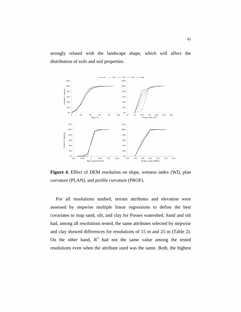
41
strongly related with the landscape shape, which will affect the
distribution of soils and soil properties.
Figure 4. Effect of DEM resolution on slope, wetness index (WI), plan
curvature (PLAN), and profile curvature (PROF).
For all resolutions studied, terrain attributes and elevation were
assessed by stepwise multiple linear regressions to define the best
covariates to map sand, silt, and clay for Posses watershed. Sand and silt
had, among all resolutions tested, the same attributes selected by stepwise
and clay showed differences for resolutions of 15 m and 25 m (Table 2).
On the other hand, R2 had not the same value among the tested
resolutions even when the attribute used was the same. Both, the highest

42
and smallest resolution presented the worst R2 values for sand, silt, and
clay. The best R2 value for all soil properties studied was the resolution of
10 m. However, the R2 values were low due the high variability of soils in
this watershed with complex slopes and only sand and clay revealed
significant linear correlation between covariates and soil properties.
Mapping sand and clay for Posses watershed the resolution of 50 m
and 10 m demonstrated the worst and the best precision, respectively
(Table 2). Once again 5 m did not show good performance reinforcing
that the desired quality of DEM depends on its application and finest
resolution is not always the best choice in DSM which agree with
Thompson et al. (2001) that suggests that higher-resolution DEM may not
be necessary for generating useful soil-landscape models.

43
Table 2. Summary of results of models developed by stepwise linear
multiple regression and precision (RMSE) of prediction for sand, silt, and
clay using a training data set (n=132) for five different resolutions of
DEM raster.
Soil
property
Resolution
(m) Attributes selected R
2 tstatistic*
RMSE
(dag kg-1
)
Sand
5 WI, elevation 30 3.713 11.51
10 WI, elevation 33 4.139 10.83
15 WI, elevation 32 3.898 11.55
25 WI, elevation 33 4.107 11.17
50 WI, elevation 24 2.905 11.85
Silt
5 WI 5 0.627 -
10 WI 6 0.728 -
15 WI 5 0.617 -
25 WI 6 0.759 -
50 WI 4 0.456 -
Clay
5 WI, elevation, slope 32 4.002 8.47
10 WI, elevation, slope 35 4.329 8.13
15 WI, elevation 33 4.042 8.25
25 WI, elevation 32 3.956 8.25
50 WI, elevation, slope 26 3.137 8.66
If tstatistic< tcritical: Accept H0; tcritical: 1.977; H0: There is no linear
relationship between soil property and environmental variables.
*Significant at the 0.05 level; WI: wetness index.
Conclusions
1. Different grid sizes of DEM were assessed and applied to verify
the effect of resolution on soil properties prediction. The characteristics of
steep slopes on study area affected the DEM model and not desired sinks
were created by the DEM on stream line for all resolutions analyzed. In

44
this case, the finest resolution was responsible for greater number of sinks
and pixels on sinks and the coarser resolution not only was better than 10
m of grid size. On the other hand, when sinks were filled, all resolutions
revealed, statistically and visually, the same pattern, except for 50 m. The
resolution of 50 m had both the worst precision and contours derived
besides formation of artifacts.
2. The effect of grid cell size on terrain derivatives were further
investigated by cumulative frequencies and all resolutions demonstrated
slight shifts except for 50 m and WI. WI had a tendency different for the
others terrain attributes reveling that this attribute is more sensible to
DEM resolution in steep landscapes. When terrain attributes and DEM
were applied on digital soil mapping to predict soil properties they
revealed that the finest resolution does not improve the prediction.
Otherwise, the small pixel size together with coarser resolution showed
worse precision.
3. In general, among all resolutions tested the grid size of 10 m
revealed to be the most stable and appropriate to use on DSM for this
watershed. It was capable to delineate relief features and soil properties
with better precision. The knowledge about the effects of resolution of
input variables on DSM is very important and proved that the smallest
resolution should not be considered always the best choice.
Acknowledgements
The authors would like to thank the Brazilian Coordination for the
Improvement of Higher Education Personnel – CAPES, the Brazilian

45
National Council for Scientific and Technological Development – CNPq
(Process no471522/2012-0 and 201987/2012-0), and Minas Gerais State
Research Foundation – FAPEMIG (Process no CAG-APQ-01423-11 and
CAG-PPM-00422-13) for funding, as well as municipal government of
City of Extrema (MG) on behalf of Director of Department of
environment Paulo Henrique Pereira to support the data collection.
References
BAENA, L. G. N., SILVA, D. D. DA, PRUSKI, F. F. & CALIJURI, M.
L. Regionalização de vazões com base em modelo digital de
elevação para a bacia do Rio Paraíba do Sul. Eng. Agríc., 24:612–
624, 2004.
CAVAZZI, S., CORSTANJE, R., MAYR, T., HANNAM, J. & FEALY,
R. Are fine resolution digital elevation models always the best
choice in digital soil mapping? Geoderma, 195-196:111–121, 2013.
CHAGAS, C. & FILHO, E. F. Avaliação de modelos digitais de elevação
para aplicação em um mapeamento digital de solos. Rev. Bras. Eng.
Agríc. Ambient., 21:218–226, 2010.
ENVIRONMENTAL SYSTEMS RESEARCH INSTITUTE – ESRI.
ArcGIS Professional GIS for the desktop, version 9.3. Redlands,
2009. CD ROM.
FLORINSKY, I., EILERS, R. ., MANNING, G. & FULLER, L.
Prediction of soil properties by digital terrain modelling. Environ.
Modell. Softw., 17:295–311, 2002.
HENGL, T. Finding the right pixel size. Comput. Sci. Eng., 32:1283–
1298, 2006.
HUTCHINSON, M. F. A new procedure for gridding elevation and
stream line data with automatic removal of spurious pits. J. Hydrol.,
106:211–232, 1989.
INSTITUTO BRASILEIRO DE GEOGRAFIA E ESTATÍSTICA. Carta
do Brasil. Rio de Janeiro, 1973. 1 mapa. Escala: 1:50000.
JENNY, H. Factors of soil formation. New York, McGraw-Hill, 1941.
109p.

46
KIENZLE, S. The Effect of DEM Raster Resolution on First Order,
Second Order and Compound Terrain Derivatives. Trans. GIS,
8:83–111, 2004.
MCBRATNEY, A., MENDONÇA-SANTOS, M. & MINASNY, B. On
digital soil mapping. Geoderma, 117:3–52, 2003.
MEDEIROS, L. C., FERREIRA, N. C. & FERREIRA, L. G. Assessment
of Digital Elevation Models for Automated Watersheds
Delimitation. Rev. Bras. Cart., 61:137–151, 2009.
MENDONÇA-SANTOS, M. L., DART, R. O., SANTOS, H. G.,
COELHO, M. R., BERBARA, R. L. L. & LUMBRERAS, J. F.
Digital Soil Mapping of Topsoil Organic Carbon Content of Rio de
Janeiro State, Brazil. In: BOETTINGER, J. L. et al., ed. Digital soil
mapping: bridging research, environmental application, and
operation. London, Springer, 2010. 255-265p.
MOORE, I. D., GESSLER, P. E., NIELSEN, G. A. & PETERSON, G. A.
Soil Attribute Prediction Using Terrain Analysis. Soil Sci. Soc. Am.
J., 57:443, 1993.
MOORE, I., GRAYSON, R. & LADSON, A. Digital terrain modelling: a
review of hydrological, geomorphological, and biological
applications. Hydrol. Process., 5:3–30, 1991.
OLIVEIRA, A. H., SILVA, M. L. N., CURI, N., KLINKE NETO, G.,
SILVA, M. A. & ARAÚJO, E. F. Consistência hidrológica de
modelos digitais de elevação (MDE) para definição da rede de
drenagem na sub-bacia do horto florestal Terra Dura, Eldorado do
Sul, RS. Rev. Bras. Ciênc. Solo, 36:1259–1268, 2012.
THOMPSON, J. A., BELL, J. C. & BUTLER, C. A. Digital elevation
model resolution: effects on terrain attribute calculation and
quantitative soil-landscape modeling. Geoderma, 100:67–89, 2001.
WILSON, J. & GALLANT, J. Terrain analysis: Principles and
Applications. New York, John Wiley and Sons, 2000. 479p.
WISE, S. Assessing the quality for hydrological applications of digital
elevation models derived from contours. Hydrol. Process., 14:1909–
1929, 2000.
ZHANG, W. & MONTGOMERY, D. R. Digital elevation model grid
size, landscape representation, and hydrologic simulations. Water
Resour. Res., 30:1019–1028, 1994.

47
ZHU, A. X., HUDSON, B., BURT, J., LUBICH, K. & SIMONSON, D.
Soil Mapping Using GIS, Expert Knowledge, and Fuzzy Logic. Soil
Sci. Soc. Am. J., 65:1463-1472, 2001.
ZHU, A.-X., BAND, L., VERTESSY, R., & DUTTON, B. Derivation of
Soil Properties Using a Soil Land Inference Model (SoLIM). Soil
Sci. Soc. Am. J., 61:523-533, 1997.

48
ARTIGO 2 Spatial distribution of soil classes and soil properties using
geomorphons and knowledge-based inference in a steep
watershed in Minas Gerais, Brazil
RESUMO
Em bacias hidrográficas, o conhecimento da distribuição das classes de
solos e atributos do solo é frequentemente requerido para manejar solos
permitindo o seu uso sustentável. Atributos do solo assim como classes de solo
são espacialmente distribuídos na paisagem e mais comumente distribuídos
seguindo um padrão. Especialmente na região sul do estado de Minas Gerais,
onde os processos erosivos são muito ativos devido ao relevo declivoso; solos
podem ser distinguidos por sua posição na paisagem e características do relevo.
O objetivo com este estudo foi avaliar um novo método para definir classes de
relevo chamado geomorphons combinado com técnicas de mapeamento digital
de solo para determinar a distribuição espacial dos atributos do solo na sub-bacia
das Posses, Minas Gerais. Diferentes modelos para predizer atributos do solo
que incluem ou não geomorphons foram comparados como krigagem e
inferência baseada no conhecimento. Sete entre nove atributos do solo preditos
(78%) tiveram os melhores resultados para erro médio absoluto (MAE) quando
geomorphons foram aplicados. Os resultados demostraram que a posição da
paisagem mostrou alta influência na distribuição dos atributos do solo
permitindo o uso dos geomorphons em associação com modelos baseados no
conhecimento.
Palavras-Chave: Atributos do terreno. Lógicas fuzzy. Krigagem. Krigagem com
regressão. Mapeamento digital de solo.
49
ABSTRACT
In watersheds, the knowledge about the spatial distribution of soil
classes and soil properties are frequently requested to manage soils allowing for
the most sustainable use. Soil properties as well as soil classes are spatially
distributed on landscapes and most commonly distributed in a predictable
pattern. Especially on southern state of Minas Gerais, Brazil, where the erosional
processes are very active due the relief is steep; soils can be distinguished by
their landscape position and relief characteristics. The objective in this study was
to evaluate a new way to define landscape types called geomorphons combined
with digital soil mapping techniques to determine the spatial distribution of soil
properties at Posses watershed, Minas Gerais, Brazil. Different models to predict
soil properties that include or no include geomorphons were compared such as
kriging and knowledge-based inference. Seven of nine soil properties predicted
(78%) had the best results of mean absolute error (MAE) when geomorphons
landforms were applied. The results demonstrated that the landscape position
showed high influence on soil and properties distribution allowing use of
geomorphons in association with knowledge-based models.
Key words:Terrain attributes. Fuzzy logic. Kriging. Regression kriging. Digital
soil mapping.

50
1 INTRODUCTION
Spatial distribution of soil properties provides essential information that
can be useful for evaluating soil fertility, water storage capacity, agricultural
planning, and natural resources management. In watersheds, the knowledge of
soil properties and the spatial distribution of soil properties are frequently
requested to manage soils allowing for the most sustainable use. In a study by
Kar, Kumar e Singh (2009) used the spatial variability of hydro-physical
properties associated with morphometric parameters to suggest sustainable
cropping systems which were more productive and lucrative in rice areas for a
watershed in India. Wang et al. (2009) and Fang et al. (2012) observed that land
use had a significant effect on the spatial variability of organic carbon content in
different watersheds in the Loess Plateau, China. Based on relationships between
carbon and environmental landscapes factors, Vasques et al. (2010) identified
soil depth, land use, soil class, stream drainage, and geology are the major
factors responsible for regional spatial patterns of total carbon in a subtropical
catchment. The soil carbon information provided information to support current
efforts to avoid loss of carbon, to improve soil fertility, and maintain the
conservation of soil resources in Florida.
Soil properties as well as soil classes are spatially distributed on
landscapes and most commonly distributed in a predictable pattern. Some
regions have high soil-landscape relationships while other areas these
relationships are less evident. In tropical regions such as Brazil, where the soil
forming factors are very active, relief plays an important role on time control of
exposure of soils on agents bioclimatic (RESENDE et al., 2007). On the oldest
surface of relief (plateau), the soils are exposed to weathering and leaching for a
longer periods of time and results in the highly weathered tropical soils

51
(Oxisols). On the other hand, in youngest and steepest surfaces, the soils will be
less developed because the erosional processes removes soil on the slopes and
deposits soils in the toeslope and footslope positions. The subsurfaces
commonly contain cambic horizons and have less development due to the active
pedogenic processes. More specifically, on southern state of Minas Gerais, the
erosional processes are very active due the relief is steep and soils can be
distinguished by their landscape position (RESENDE et al., 2007). The
following soils can be linked to specific landforms: 1) highly weathered tropical
soils (Oxisols) can been found on gentle and continuous slopes (summits), 2)
argillic horizons on shoulders and summits of irregular and discontinuous
landscapes, 3) weakly developed and shallow soils (Inceptisols and Entisols –
associated with rock outcrop) on very unstable and steep landscapes (shoulders,
backslope), and 4) depositional and alluvial soils on deposition areas and
floodplains (footslope, valleys) (RESENDE et al., 2007).
The strong relationships between soils and landscape are the key for
traditional polygon based soil mapping in several parts of the world, including
Brazil. However, the polygon based map considers spatial variation of soils only
occur at the boundaries of delineated polygons, thus, soil properties have
uniform values within each soil polygon (ZHU et al., 1997, 2001). Even though
field experience shows us that abrupt changes of soils over space exist, more
often this is gradual and continuous unlike polygon-based mapping (ZHU et al.,
2001). Advances in geographic information systems (GIS) over the past 30 years
has allowed for the advent of newer techniques using raster instead of polygons.
This raster based technique, commonly called Digital Soil Mapping (DSM), is
based on the relationships among soils and the factors and processes of soil
formation (clime, organisms, relief, parent material, and time - CLORPT)
according to Jenny (1941) that are entered in the equations as predictor variables

52
(MENDONÇA-SANTOS et al., 2010). Many soil scientists have studied DSM
techniques to improve the predictive spatial variability of soils properties for a
variety of regions according there unique environmental characteristics.
McBratney, Mendonça Santos and Minasny, (2003) discussed various methods
that have been used to identify relationships between soil properties and
environmental variables including linear models, classification and regression
trees, fuzzy membership models, neural networks, and geostatistics. Zhu et al.
(1997, 2010) applied different approaches to map soil properties using fuzzy
membership model from the environmental variables. Using geostatistics and
fuzzy logic, Menezes (2011) discovered relationships between soil classes and
environmental variables while mapping soil properties and predicted
groundwater recharge potential in watersheds in Brazil. Veronese Júnior et al.
(2006) applied geostatistics to explain the spatial variability of the mechanical
resistance to penetration and gravimetric moisture in a Ferralsol in Brazil.
Oliveira et al. (2012) applied the relationships between soil and environmental
variables in linear regression models to predict organic matter content at Salto
watershed in Extrema, Minas Gerais.
To describe the physiographical variability, landscape covariates (terrain
attributes) are derived from a digital elevation model (DEM) which includes
terrain curvature, slope, topographic wetness index, etc. These attributes are a
function of differential geometry and they do not consider the occurrence of soil
according landscape position, but only the relationships among these derivatives
and soil class. In compliment of this methodologies Jasiewicz and Stepinski
(2013) developed a novel approach to landform classification called
geomorphons which is based on the principle of pattern recognition rather than
differential geometry. Geomorphons classify the landform using the concept of
local ternary patterns (LTP) (LIAO, 2010) deriving from a base DEM the 10

53
common landform types: peak, ridge, shoulder, spur, hollow, footslope, valley,
pit, and flat with a small computational cost (JASIEWICZ; STEPINSKI, 2013).
Geomorphons and landscape covariates are easily generated from a DEM.
Terrain attributes have been used in several studies and have showed good
performance to predict soil properties (BOER; DEL BARRIO;
PUIGDEFÁBRES, 1996; MOORE et al., 1993; MOTAGHIAN;
MOHAMMADI, 2011; ODEH; McBRATNEY; CHITTLEBOROUGH, 1995;
WINZELER et al., 2008).
The overarching hypothesis for this research is that landform has very
strong influence on occurrence of soils and properties on steep landscapes at
Minas Gerais, Brazil. The objective in this study was to evaluate the pattern
recognition application of geomorphons combined with DSM techniques to
determine the spatial distribution of soil properties at Posses watershed, Minas
Gerais, Brazil.

54
2 MATERIAL AND METHODS
2.1 Study area
The study was conducted at Posses watershed (46°14’W and 22°51’S),
which is located at the city of Extrema, southern of Minas Gerais, Brazil, and
covers an area of 12 km2 (Figure 1). The climate in this region, according to the
Köppen climate classification, is Cwb (temperate highland tropical climate with
dry winters) with average temperature ranging from 13°C to 26°C and an
average annual precipitation of 1,477 mm the wettest period is from October to
March and the dry period from April to September. The original ecosystem in
this watershed was Atlantic Forest (Tropical Rain forest), which was has largely
been replaced by pastures (> 70% of area). This watershed is located on
southern end of the Mantiqueira Mountains Range with elevation ranging from
968 m to 1,420 m, and characterized by steep relief.

55
Figure 1 Study area location, biome, and soil samples distribution on the
elevation (m) map at 10m resolution
The dominant soils classes classified according to Brazilian Soil
Classification System (EMPRESA BRASILEIRA DE PESQUISA
AGROPECUÁRIA - EMBRAPA, 2006) are Red-Yellow Argisol (PVA), Humic
Cambisol (CH), Haplic Cambisol (CX), Lithic Neosol (RL), and Fluvic Neosol
(RY) developed from gneiss-granite.
2.2 Field sampling and laboratory analysis
The surface soil (0-20 cm) was randomly sampled in the whole
watershed for a total of 141 disturbed samples and 161 undisturbed samples (20
samples from soil survey and 141 randomly sampled). Disturbed samples were

56
collected by dig the soil profile without preserve the soil structure and
undisturbed samples were sampled using the Uhland sampler to preserve the soil
structure. A (GARMIN eTrex Vista) global positioning system (GPS) was used
to get the coordinates of all the sample locations. These samples were split in
two sets. The first was an interpolation set (112 disturbed samples and 132
undisturbed samples) and the second was a validation set (29 disturbed samples
and 29 undisturbed samples) (Figure 1). The validation set was approximately
20% of the total samples and was used to check the accuracy of the interpolation
data set predictability.
Analysis of the undisturbed samples included sand, silt, and clay content
using the Hydrometer Method (GEE; BAUDER, 1986), organic matter (OM)
according to Walkley and Black (1934), and particle density (PD) by the
Pycnometer Method (BLAKE; HARTGE, 1986). Methods for analyzing the
undisturbed samples were saturated hydraulic conductivity (Ksat) using a
permeameter of constant load (LIMA et al., 1990), bulk density (BD) based on
soil samples of known volume (BLAKE; HARTGE, 1986), microporosity
(MIC) which corresponds to the moisture retained up to a tension of 0.006 MPa,
determined by a porous plate apparatus (DANIELSON; SUTHERLAND, 1986),
macroporosity (MAC) obtained from the difference between total porosity (TP)
and MIC, and TP calculated from the values of BD and PD using the equation
according to EMBRAPA (1997).
2.3 Prediction of spatial variability of soil properties
To verify the performance of models that combine geomorphons with
DSM technics, soil properties (sand, silt, clay, OM, BD, TP, MIC, MAC, and
Ksat) were predicted by models using geomorphons and models that do not use
57
geomorphons. Two types of models were chosen: statistical models and
knowledge-based inference. The statistical models were kriging (MATHERON,
1971) which is a powerful interpolator based on geostatistics that allows
predicting complex spatial patterns by considering soil variables have a spatial
structure (regionalized variables). This method uses statistics to calculate the
unsampled areas by modeling the spatial dependence between neighboring
observations as a function of their distance (THOMPSON; BELL; BUTLER,
2012). The knowledge-based inference used was Soil Land Inference Model
(SoLIM), based on fuzzy logic (ZHU; BAND, 1994; ZHU et al., 1996, 1997,
2001; ZHU, 1997) which uses expert knowledge of experienced soil scientist to
formalize the relationship between soil characteristics and environmental
variables.
2.3.1 Environmental variables
Due to the relatively small size of the study area, the Jenny equation
factors: climate, organisms, and parent material were considered constants.
Considering the time is related with landscape evolution, which varies among
different regions, the factor relief was considered to be the major driver of
pedogenesis and therefore was used as environmental variables. A base digital
elevation model (DEM) with 10m of resolution was used to develop the
landscape covariates (Chapter 1).
Two sets of environmental variables created from DEM were used: The
terrain attributes (TA) that refer to the environmental variables are developed by
differential geometry and include (a) Slope defined as the gradient or rate of
change of elevation; (b) SAGA wetness index (WI) which is a wetness index
similar to the topographic wetness index (TWI) (BEVEN; KIRKBY, 1979). This

58
index is based on a modified catchment area calculation, which does not
consider the flow as very thin film (BÖHNER et al., 2002); (c) Plan curvature
(PLAN) which is defined as being transverse to the slope and measures the
convergence or divergence and hence the concentration of water in a landscape
(MOORE et al., 1993); and (d) Aspect which is defined as the orientation of the
line of steepest descent and is usually measured in degrees clockwise from north
(WILSON; GALLANT, 2000) (Figure 2a).
The other environmental covariate describing terrain was Geomorphons
(GEOM). This classification identifies landforms types based on concept of
local ternary patterns (LTP) (LIAO, 2010) which utilizes a line-sight
neighborhood (LEE, 1991; NAGY, 1994; YOKOYAMA; SHIRASAWA; PIKE,
2002) instead of a fixed-scale window to extract information about the surface
(JASIEWICZ; STEPINSKI, 2013). Geomorphons were derived from a single
scan of the DEM using two parameters as input: look up distance (L) of 50 cells
(500m) and flatness threshold (t) of 1 degree (Figure 2b). Of the ten
geomporphons landforms available only six were recognized for Posses
watershed (Figure 2b). The software used to develop the environmental
variables were SAGA GIS 2.0.8 (BÖHNER et al., 2013), ArcGIS 9.3
(ENVIRONMENTAL SYSTEMS RESEARCH INSTITUTE - ESRI, 2009), and
GRASS GIS 7.0 (NETELER; MITASOVA, 2008). The code for processing
geomorphons can be found at University of Cincinnati (2013).

59
Figure 2 Environmental variables: (a) slope (%), wetness index (WI), plan
curvature (PLAN), and aspect, and (b) landform types
(geomorphons), for the Posses watershed, Minas Gerais, Brazil.
2.3.2 Kriging
Kriging determines values for points with unknown values and
correlating these points and their neighbors through the semivariogram by
obtaining weights of varying distances (MATHERON, 1963, 1971). The
semivariogram is a curve representing the degree of continuity of a variable
using the following expression (MATHERON, 1963):

60
n
ihssz
hnh
1
2^
)]()([)(2
1
Where h^
is the estimated value of semivariance between pairs of
points z(s) and z(s+h); z(s) and z(s+h) are values of variable z at the positions s
and s+h, respectively; and n(h) is the number of pairs of points separated by the
same distance h.
After the calculation of the semivariogram, ordinary kriging (standard
version of kriging) could be used to predict the soil properties for the Posses
watershed using the following equation (MATHERON, 1963, 1971).
in
i i szsz
1
^
0
Where ^
0sz is the estimated value for a location (s0) not sampled; z(si)
is the variable sampled; and λi are the weights associated with the semivariance
of the sampling points. The weights sum to unity is a condition which indicates
unbiased estimation.
Commonly, exhaustive field sampling for soils is required for ordinary
kriging (OK) because points sampled closer to one another will be more related.
However exhaustive field sampling is not always possible due high cost of
sample analysis, people hours and time requirements. Some hybrids of kriging
have been applied to minimize intense sample needs such as regression kriging
(RK). The regression kriging combines multiple linear regression and ordinary

61
kriging (BISHOP; McBRATNEY, 2001; HENGL; HEUVELINK; ROSSITER,
2007; ODEH; McBRATNEY; CHITTLEBOROUGH, 1994, 1995; ZHU; LIN,
2010). Three steps to predict soil properties by RK was used: 1) stepwise
multiple linear regression model between the target variable and environmental
variables was developed; 2) the residuals from multiple linear regression
between the target variable and environmental variables were interpolated using
ordinary kriging; 3) the regressed values and kriged residuals were added
together at unknown value as the predicted values (ODEH; McBRATNEY.;
CHITTLEBOROUGH, 1995).
All of the geostatistical analysis (stepwise multiple linear regression,
semivariograms, OK, and RK) was determined in the R environment (R
DEVELOPMENT CORE TEAM, 2010).
2.3.3 SoLIM
SoLIM is a predictive approach to soil mapping that uses a combination
of expert knowledge of the soil scientist and data analysis to input information
about soils and their related environmental variables. This application used
within a GIS environment results in fuzzy membership (similarity) maps (ZHU
et al., 1997, 2001) based on fuzzy membership classification. Fuzzy membership
maps can be hardened which generates a soil class map of the highest fuzzy
membership values for a given point (ZHU, 1997). In this study, the Rule-Based
Reasoning (RBR) inference was used to define the relationship between values
of an environmental variable and a given soil class (ZHU; BURT; DU, 2010).
Three different options to create membership maps were tested on the Posses
watershed which considered the dominant soil classes that occur in the research
area (PVA, CX, CH, RL, and RY) according to the soil survey:

62
1) Terrain attributes (TA): Soil survey (Figure 1) information,
knowledge of the soils occurrence, and terrain attributes (elevation, slope, WI,
PLAN, and aspect) (Figure 2a) to define the soil-environment relationships as
rules (RBR) was used for this option;
2) Geomorphons (GEOM): Rules were defined based on soil survey
(Figure 1) information and the knowledge of the soil landscape relationships,
where each soil class was associated with the landform types (Figure 2b).
However, for landform slope (Figure 2b), it was not possible associate just one
soil class because more than one soil class (CH, CX, PVA, RL) occurs on this
landform type. In this case, the terrain attributes slope, elevation, and PLAN
were used together with geomorphons to define the rules;
3) Geomorphons (GEOM) combined with terrain attributes (TA)
(GEOM-TA): In this case, the rules were defined using soil survey (Figure 1)
information, TA (Figure 2a), and GEOM (Figure 2b). Using the knowledge of
the soils occurrence on landscape and soil data information from soil survey,
geomorphons landform was associated with each soil class. Then, slope, PLAN,
and elevation were used to define the soil-environment relationships as rules
(RBR).
Thus, after creating the membership maps, the soil properties maps for
sand, clay, OM, BD, TP, MIC, MAC, and Ksat could be developed according
the following linear and additive weighting function (ZHU et al., 1997):
n
k
k
ij
kk
ij
n
k
ij
S
VSV
1
1

63
Where Vij is the property value at location (i,j), k
ijS is the fuzzy
membership value at (i,j) for soil class k, n is the total number of soil classes, Vk
is the typical property value of soil on class k.
To define the typical property value of soil in class k for TA, GEOM,
and GEOM-TA three different tests were applied (ZHU et al., 2010). (1) Highest
membership (HM) used the average property values observed at a field location
that corresponded to the highest fuzzy membership value for each soil class for
all field observations; (2) Regression membership (RM) tested a multiple linear
regression between observed soil properties at field and the fuzzy membership
values to predict the soil property value at a given location; (3) Typical (T) used
the average property values observed at field location for each soil class.
2.4 Models assessment
The prediction was assessed by comparing the predicted values with the
correspondent values from the validation set through the mean absolute error
(MAE) which should be closest to 0.
n
szszMAE
n
j jj
1
^
||
Where n is the number of validation points;
^
z js is the estimated
values at point j; and z js is the validation value at point j.

64
3 RESULTS AND DISCUSSION
Considering the large number of potential environmental variables, the
stepwise multiple linear regression was used to verify the best multiple linear
regression model to use on regression kriging (RK) (Table 1). Results showed
low linear correlation between soil properties and terrain attributes represented
by the small R2 values that ranged from 0.07 to 0.4. Also, for the properties BD,
TP, and Ksat were not possible to develop the linear regression equations
because no one of environmental variables showed correlation with these soil
properties. Even though some studies has showed that RK normally outperform
OK even with small R2 values (BISHOP; McBRATNEY, 2001; MENEZES,
2011; MOTAGHIAN; MOHAMMADI, 2011) none of these studies has tested if
the linear correlation is significant. It might will be relevant to consider the
possibility that an apparent trend in the data is illusory and reflects only
sampling variability (SAMUELS; WITMER; SCHAFFNER, 2012). In this
study the Student’s t test was applied to make sure that has not linear correlation
between soil properties and environmental variables with small R2 values on
Posses watershed. So, Student’s t test proved that only sand and clay have linear
relationship with environmental variables allowing the use of the RK to predict
these properties.

65
Table 1 Stepwise multiple linear regression models between soil properties
and environmental variables for Posses watershed, Minas Gerais,
Brazil
Parameters Sand Silt Clay OM MIC MAC
------------------------------------%-------------------------------------------
Intercept -40.62 36.29 81.81 5.24 40.67 13.36
Slope - - - - - -
WI 3.27 -0.86 -1.94 -0.16 - -
Elevation 0.04 - -0.02 - - -
PLAN 1,112.37 - -959.1 -114.92 1,186.93 -1,230.80
R2 0.40 0.08 0.29 0.17 0.08 0.07
sample size 132 132 132 132 112 112
ttable* 1.977 1.977 1.977 1.977 1.984 1.984
tstatistic 4.976 0.915 3.455 1.967 0.842 0.736
*Significant at the 0.05 level. If tstatistic< ttable: Accept H0. H0: There is no linear
relationship between soil properties and environmental variables. Organic matter (OM);
microporosity (MIC); macroporosity (MAC); wetness index (WI); plan curvature
(PLAN).
The semivariograms fitted for each soil property as well as for the
residuals of multiple linear regression are presented on Figure 3. All, variables,
except Ksat presented some spatial dependence that allowed kriging of the soil
properties. Ksat presented pure nugget effect (semivariance random) which
means the data are independent and they have no spatial dependence. The spatial
dependence is a requirement in geostatistics because this method requires that
the relationship between the value at one point and any sample value depends on
the distance between the two positions (CLARK, 1979).
Another important observation is that all experimental semivariograms
presented nugget effect represented by the discontinuity at the origin of the
experimental semivariograms (MATHERON, 1963). This effect reflects the
66
spatial variability not captured by the field sampling. It also suggests that the
field sampling was limited which reduces the ability to capture all of the
variability that exists for those variables having a consequential increase of the
variance with the reduction of samples (MATHERON, 1971).
Subsequently, it was not possible to capture the spatial structure for Ksat
resulting in pure nugget effect which probably could be resolved or improved
with a bigger sampling pool. Studies have showed the Ksat is highly variable
making it difficult to study spatially by using geostatistics (MENEZES, 2011;
MOUSTAFA, 2000). The use of nonlinear transformations to get spatial
structure by modeling Ksat through geostatistics analysis may be a viable option
(HERBST; DIEKKRÜGER, B; VEREECKEN, 2006; MENEZES, 2011).
However, when data are transformed using nonlinear transformations the shape,
frequency, distribution, mean, and standard deviation of the data change after
transformations affecting the data (SAMUELS; WITMER; SCHAFFNER,
2012). Thus, for this study, transformations were not utilized and the original
structure of data was maintained to avoid changes on data structure. It is not
make sense change the structure of the data if our focus is analyzing the
variability of the data.

67
Figure 3 Experimental semivariograms (points) and semivariogram estimated
by the models (lines) of soil properties
3.1 Assessment of prediction models
Table 2 shows the mean absolute error (MAE) values for predictive
models suggesting good performance of the geomorphons. Only silt and MIC

68
did not provide statistically significant predictions with geomorphons. SoLIM
proved to be more robust than kriging because it was the best predictor for all
soil properties, except silt. Kriging requires a large number of samples to obtain
all the variability for any given data set and become less predictive when the
study area is a watershed with steep landscape. To resolve this issue and
improve the results RK can be applied if linear relationship exists between target
variable and environmental variables (BISHOP; McBRATNEY, 2001; ODEH;
McBRATNEY; CHITTLEBOROUGH, 1994, 1995). In this study, RK
improved the results of KO only for sand and OK was better to predict clay.
According to Hengl, Heuvelink and Rossiter (2007) when auxiliary information
is available RK outperforms OK because it exploits the extra information, but
this auxiliary information should explain part of the variation in the target
variable. However, this was not the case in this study for clay, due the lower R2
values. Also, Zhu and Lin (2010) support the notion that RK outperforms OK
when the relationship between soil property and environmental variables are
strong (R2> 0.6). Bishop and Mcbratney (2001) found greater precision of the
models when them had bigger correlation between target variable and the
secondary variable. Soils in this watershed have high spatial variability and low
linear relationship between topographic variables due to the high level of
erosion. To improve these models it requires a big data sampling data set for
kriging, however, the minimal data set for this study had resulted in the a weaker
estimate when using KO and RK as compared to using SoLIM.
SoLIM was used to overcome the sample limitations because it applies
expert knowledge of soil-landscape relationships and it does not require linear
relationships (ZHU et al., 2001, 2010). Moreover, SoLIM had its performance
improved when geomorphons were applied as environmental variable for all
properties except for MIC and silt. These results suggest that relationships

69
between soils and landform do exist in this region, they are not linear, and they
can improve the models when landscape position is considered. They also
showed that the geomorphons worked better when associated with terrain
attributes for sand, clay, BD, MAC, and Ksat. The Posses watershed has a steep
slope and high relief which is a result of erosional process and geomorphons has
provided a good covariate for representing the soil landscape relationships.
MENDONÇA-SANTOS et al. (2010) found strong correlation between organic
carbon, soil type, and its position on this landscape in Rio de Janeiro, Brazil
which coincides with the results of this study.
Comparing the different options tested to define the typical property
value per soil class, the results showed that the T (average property values
observed at field location for each soil class mapped) performed better. Seis of
nine (66%) of the soil properties had better performance when T was used. HM
also showed good results and had the best values of MAE in 33% of the results.
On the other hand, RM did not predict soil properties as accurately when used in
SoLim. The RM was limited to use only for sand, silt, clay, and OM because the
linear regression between membership maps and BD, TP, MIC, MAC, and Ksat
were not significant. Zhu et al. (2010) concluded that RM works well over areas
where soil environmental relationships are more complicated and HM can serve
as a viable option for soil property prediction over large areas. However our
results do not agree with these conclusions. The issue to use RM is because the
linear correlation is required and it was not possible for the majority of the soil
properties studied.

70
Table 2 Mean absolute error (MAE) for prediction models
Model Sand Silt Clay OM BD TP MIC MAC Ksat
KO 2.1 0.96 2.77 0.54 0.012 0.31 0.72 0.19 -
RK 1.85 - 3.05 - - - - - -
TAHM 0.46 1.80 2.26 0.31 0.004 0.18 0.04 0.22 0.94
TARM 0.58 1.86 2.44 0.31 - - - - -
TAT 0.50 1.74 2.23 0.38 0.004 0.18 0.33 0.15 1.02
GEOMHM 0.23 2.03 1.79 0.29 0.002 0.05 0.18 0.23 1.16
GEOMRM 0.62 2.27 1.66 0.31 - - - - -
GEOMT 1.36 2.88 1.52 0.23 0.003 0.02 0.53 0.51 1.74
GEOM-TAHM 0.46 1.90 1.43 0.30 0.003 0.26 0.44 0.18 0.93
GEOM-TARM 0.68 2.40 1.72 0.30 - - - - -
GEOM-TAT 0.05 1.98 2.03 0.34 0.001 0.18 0.15 0.03 1.17
KO: ordinary kriging; RK: regression kriging; TAHM: terrain attribute as rule and
highest membership as typical property value; TARM: terrain attribute as the rule and a
regression membership as the typical property value; TAT: terrain attribute as the rule
and the average value as typical property value; GEOMHM: geomorphons as the rule
and highest membership as the typical property value; GEOMRM: geomorphons as the
rule and regression membership as the typical property value; GEOMT: geomorphons as
the rule and the average value as the typical property value; GEOM-TAHM:
geomorphons and terrain attribute as the rule and highest membership as the typical
property value; GEOM-TARM: geomorphons and the terrain attribute as the rule and a
regression membership as the typical property value; GEOM-TAT: geomorphons and
other terrain attribute as the rule and the average value as the typical property value;
OM: organic matter; BD: bulk density; TP: total porosity; MIC: microporosity; MAC:
macroporosity; Ksat: saturated hydraulic conductivity.
3.2 Prediction of soil properties and soil classes
The soil classes and soil property maps can be viewed in Figure 4. The
hardened map (soil map) for this watershed was created using membership maps
developed by GEOM-TA model due its better performance for five of nine
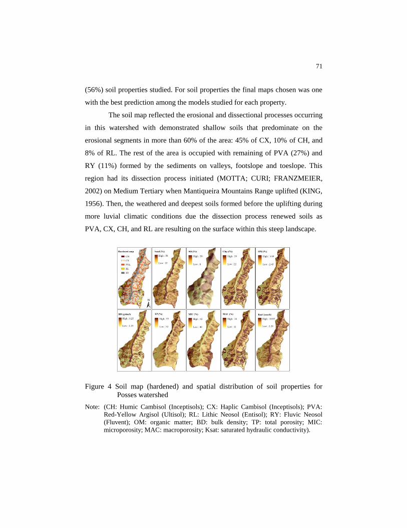
71
(56%) soil properties studied. For soil properties the final maps chosen was one
with the best prediction among the models studied for each property.
The soil map reflected the erosional and dissectional processes occurring
in this watershed with demonstrated shallow soils that predominate on the
erosional segments in more than 60% of the area: 45% of CX, 10% of CH, and
8% of RL. The rest of the area is occupied with remaining of PVA (27%) and
RY (11%) formed by the sediments on valleys, footslope and toeslope. This
region had its dissection process initiated (MOTTA; CURI; FRANZMEIER,
2002) on Medium Tertiary when Mantiqueira Mountains Range uplifted (KING,
1956). Then, the weathered and deepest soils formed before the uplifting during
more luvial climatic conditions due the dissection process renewed soils as
PVA, CX, CH, and RL are resulting on the surface within this steep landscape.
Figure 4 Soil map (hardened) and spatial distribution of soil properties for
Posses watershed
Note: (CH: Humic Cambisol (Inceptisols); CX: Haplic Cambisol (Inceptisols); PVA:
Red-Yellow Argisol (Ultisol); RL: Lithic Neosol (Entisol); RY: Fluvic Neosol
(Fluvent); OM: organic matter; BD: bulk density; TP: total porosity; MIC:
microporosity; MAC: macroporosity; Ksat: saturated hydraulic conductivity).

72
4 CONCLUSIONS
Soil properties in this watershed presented low linear correlation
between soils and environmental variables. They also showed weak spatial
dependence between samples requesting greater number of points sampled for
kriging. However, the minimal data set for this study had resulted in an
improvement of the accuracy of maps when SoLIM were used demonstrating
superiority over kriging methods.
Soil properties as well as soils classes are distributed according to
landscape position which has been the result of erosion processes which
modifies the landscape by parallel slope retreat. The highest sand content, Ksat,
and BD is on RY. This region due the higher precipitation, deeper and
weathered mantle, and intense dissection is highly eroded by streams that are the
primary process carrying fine sandy sediments to the lowlands. Clay, OM and
MAC followed the same pattern: higher OM where the clay content is high and
lower content of OM and clay on steep slope. However, BD as well as TP and
MIC did not show extreme variations in their distributions for the watershed, but
represented smaller areas with more concentration of these properties when
compared to the rest of the watershed. For TP the highest values were on PVA
located at lower elevations while the highest MIC values were at higher
elevations and on steeper slopes. These soils have good granular structure and in
general are clayey, except RY. The granular structure results in higher
permeability and the OM helps to maintain the soil particles in the aggregates
(OM works as cementing agent on the aggregates) reducing susceptibility to
erosion; however on steep slopes these aggregates can rupture, releasing the soil
particles that can rearrange forming crusts and increasing their erodibility.

73
In general, the landscape position showed high influence on soil and
properties distribution allowing use of geomorphons in association with
knowledge-based models. These results confirm the hypothesis that landform
has very strong influence on occurrence of soils and properties on steep
landscapes at Minas Gerais. The soil position on landscape should be considered
to map soils as well as to suggest management practices in steep sloping
landscapes in tropical regions.

74
REFERENCES
BEVEN, K. J.; KIRKBY, M. J. A physically based, variable contributing area
model of basin hydrology / Un modèle à base physique de zone d’appel variable
de l'hydrologie du bassin versant. Hydrological Sciences Bulletin, London, v.
24, n. 1, p. 43-69, Mar. 1979.
BISHOP, T.; McBRATNEY, A. A comparison of prediction methods for the
creation of field-extent soil property maps. Geoderma, Amsterdam, v. 103, n.
1/2, p. 149-160, Sept. 2001.
BLAKE, G. R.; HARTGE, K. H. Bulk density. In: KLUTE, A. (Ed.). Methods
of soil analysis. 2nd ed. Madison: American Society of Agronomy, 1986. p.
363-375.
BOER, M.; DEL BARRIO, G.; PUIGDEFÁBRES, J. Mapping soil depth
classes in dry Mediterranean areas using terrain attributes derived from a digital
elevation model. Geoderma, Amsterdam, v. 72, n. 1/2, p. 99-118, July 1996.
BÖHNER, J. et al. Soil regionalization by means of terrain analysis and process
parameterization. In: MICHELI, E. et al. (Ed.). Soil classification 2001.
Luxembourg: European Soil Bureau, 2002. p. 213-222. (Research Report No. 7,
EUR 20398 EN).
BÖHNER, J. et al. System for an automated geographical analysis. 2001.
Available at: <http://www.saga-gis.org>. Access in: 21 May. 2013.
CLARK, I. Practical geostatistics. London: Elsevier Applied Science
Publishers, 1979. 129 p.

75
DANIELSON, R. E.; SUTHERLAND, P. L. Porosity. In: BLACK, C. A. (Ed.).
Methods of soil analysis I: physical and mineralogical methods. Madison:
American Society of Agronomy/Soil Science Society of America, 1986. p. 443-
461.
EMPRESA BRASILEIRA DE PESQUISA AGROPECUÁRIA – EMBRAPA.
Centro Nacional de Pesquisa de Solos. Sistema brasileiro de classificação de
solos. Rio de Janeiro, 2006. 306 p.
EMPRESA BRASILEIRA DE PESQUISA AGROPECUÁRIA – EMBRAPA.
Manual de métodos de análises de solo. 2. ed. Rio de Janeiro, 1997. 212 p.
ENVIRONMENTAL SYSTEMS RESEARCH INSTITUTE - ESRI. ArcGIS
Professional GIS for the desktop, version 9.3. Redlands, 2009. 1 CD-ROM.
FANG, X. et al. Soil organic carbon distribution in relation to land use and its
storage in a small watershed of the Loess Plateau, China. Catena, Amsterdam,
v. 88, n. 1, p. 6-13, Jan. 2012.
GEE, G. W.; BAUDER, J. W. Particle-size analysis. In: KLUTE, A. (Ed.).
Methods of soil analysis. Part 1. Physical and mineralogical methods. 2nd ed.
Madison: American Society of Agronomy/ Soil Science Society of America,
1986. p. 383-411.
HENGL, T.; HEUVELINK, G. B. M.; ROSSITER, D. G. About regression-
kriging: from equations to case studies. Computers & Geosciences,
Amsterdam, v. 33, n. 10, p. 1301-1315, Oct. 2007.
HERBST, M.; DIEKKRÜ, B.; VEREECKEN, H. Geostatistical co-
regionalization of soil hydraulic properties in a micro-scale catchment using
terrain attributes. Geoderma, Amsterdam, v. 132, n. 1/2, p. 206-221, May 2006.
JASIEWICZ, J.; STEPINSKI, T. F. Geomorphons — a pattern recognition
approach to classification and mapping of landforms. Geomorphology,
Amsterdam, v. 182, n. 1 , p. 147-156, Jan. 2013.

76
JENNY, H. Factors of soil formation. New York: McGraw-Hill, 1941. 109 p.
KAR, G.; KUMAR, A.; SINGH, R. Spatial distribution of soil hydro-physical
properties and morphometric analysis of a rainfed watershed as a tool for
sustainable land use planning. Agricultural Water Management, Amsterdam,
v. 96, n. 10, p. 1449-1459, Oct. 2009.
KING, L. C. A geomorfologia do Brasil Oriental. Revista Brasileira de
Geografia, Rio de Janeiro, v. 18, n. 2, p. 147-265, 1956.
LEE, J. Analyses of visibility sites on topographic surfaces. International
Journal of Geographical Information Systems, London, v. 5, n. 4, p. 413-429,
Jan. 1991.
LIAO, W-H. Region description using extended local ternary patterns. In:
INTERNATIONAL CONFERENCE ON PATTERN RECOGNITION, 20.,
2010, Istanbul. Anais... Istanbul: IEEE, 2010. Disponível em:
<http://ieeexplore.ieee.org/lpdocs/epic03/wrapper.htm?arnumber=5595845>.
Acesso em: 21 maio 2013.
LIMA, J. M. et al. Dispersão do material de solo em água para avaliação indireta
da erodivilidade da Latossolos. Revista Brasileira de Ciência do Solo,
Campinas, v. 14, n. 1, p. 85-90, jan./abr. 1990.
MATHERON, G. Principles of geostatistics. Economic Geology, Lancaster, v.
58, n. 8, p. 1246-1266, 1963.
MATHERON, G. The theory of regionalized variables and its applications.
Fontainebleau: École Nationale Supérieure des Mines de Paris, 1971. 211 p.
McBRATNEY, A.; MENDONÇA SANTOS, M.; MINASNY, B. On digital soil
mapping. Geoderma, Amsterdam, v. 117, n. 1/2, p. 3-52, Nov. 2003.

77
MENDONÇA-SANTOS, M. L. et al. Digital soil mapping of topsoil organic
carbon content of Rio de Janeiro state, Brazil. In: BOETTINGER J. L. et al.
(Ed.). Digital soil mapping: bridging research, environmental application, and
operation. London: Springer, 2010. p. 255-265.
MENEZES, M. D. Levantamento pedológico de hortos florestais e
mapeamento digital de atributos físicos do solo para estudos hidrológicos.
2011. 225 p. Tese (Doutorado em Ciência do Solo) – Universidade Federal de
Lavras, Lavras, 2011.
MOORE, I. D. et al. Soil attribute prediction using terrain analysis. Soil Science
Society of America Journal, Madison, v. 57, n. 2, p. 443-452, Mar./Apr. 1993.
MOTAGHIAN, H. R.; MOHAMMADI, J. Spatial estimation of saturated
hydraulic conductivity from terrain attributes using Regression, Kriging, and
Artificial Neural Networks. Pedosphere, London, v. 21, n. 2, p. 170-177, Apr.
2011.
MOTTA, P. E. F.; CURI, N.; FRANZMEIER, D. P. Relation of soil and
geomorphic surfaces in the Brazilian Cerrado. In: OLIVEIRA, P. S.;
MARQUIS, R. J. (Ed.). The cerrados of Brazil: ecology and natural history of
a neotropical savanna. New York: Columbia University, 2002. p. 13-32.
MOUSTAFA, M. M. A geostatistical approach to optimize the determination of
saturated hydraulic conductivity for large-scale subsurface drainage design in
Egypt. Agricultural Water Management, Amsterdam, v. 42, n. 3, p. 291-312,
Jan. 2000.
NAGY, G. Terrain visibility. Computers and Graphics, Amsterdam, v. 18, n.
6, p. 763-773, Sept./ Oct. 1994.
NETELER, M.; MITASOVA, H. Open Source GIS: a GRASS GIS approach.
3rd ed. New York: Springer, 2008.

78
ODEH, I.; McBRATNEY, A.; CHITTLEBOROUGH, D. Further results on
prediction of soil properties from terrain attributes: heterotopic cokriging and
regression-kriging. Geoderma, Amsterdam, v. 67, n. 1, p. 215-226, Aug. 1995.
ODEH, I.; McBRATNEY, A.; CHITTLEBOROUGH, D. Spatial prediction of
soil properties from landform attributes derived from a digital elevation model.
Geoderma, Amsterdam, v. 63, n. 3/4, p. 197-214, Nov. 1994.
OLIVEIRA, A. H. et al. Caracterização ambiental e predição dos teores de
matéria orgânica do solo na Sub-Bacia do Salto, Extrema, MG. Semina:
Ciências Agrárias, Londrina, v. 33, n. 1, p. 143-154, abr. 2012. Avaiable at
<http://www.uel.br/revistas/uel/index.php/semagrarias/article/view/5914>.
Access in: 23 Jul. 2013.
R DEVELOPMENT CORE TEAM. R: a language and environment for
statistical computing. Vienna: R Foundation for Statistical Computing, 2010.
Avaiable at: <http://www.R-project.org>. Access in: 10 Dec. 2011.
RESENDE, M. et al. Pedologia: base para distinção de ambientes. 5. ed. rev.
Lavras, MG: Ed. UFLA, 2007. 322 p.
SAMUELS, M.; WITMER, J.; SCHAFFNER, A. Statistics for the life
sciences. 4th ed. Boston: Pearson, 2012. 668 p.
THOMPSON, J. A.; BELL, J. C.; BUTLER, C. A. Digital elevation model
resolution: effects on terrain attribute calculation and quantitative soil-landscape
modeling. Geoderma, Amsterdam, v. 100, n. 1/2, p. 67–89, Mar. 2001.
UNIVERSITY OF CINCINNATI. SPACE INFORMATICS LAB.
Geomorphons. Cincinnati, Ohio, 2013. Avaiable at:
<http://sil.uc.edu/downloads.html#software>. Access in: 23 Jul. 2013

79
VASQUES, G. M. et al. Regional modelling of soil carbon at multiple depths
within a subtropical watershed. Geoderma, Amsterdam, v. 156, n. 3/4, p. 326-
336, May 2010.
VERONESE JÚNIOR, V. V. et al. Spatial variability of soil water content and
mechanical resistance of Brazilian Ferralsol. Soil and Tillage Research,
Amsterdam, v. 85, n. 1/2, p. 166-177, Jan. 2006.
WALKLEY, A.; BLACK, I. An examination of the Degtjareff method for
determining soil organic matter, and a proposed modification of the chromic
acid titration method. Soil Science, Baltimore local, v. 37, n. 1, p. 29-38, 1934.
WANG, Y-Q. et al. Spatial variability of soil organic carbon in a watershed on
the Loess Plateau. Pedosphere, London, v. 19, n. 4, p. 486-495, Aug. 2009.
WILSON, J. P.; GALLANT, J. C. Primary topographic attributes. In: WILSON,
J. P.; GALLANT, J. C. (Ed.). Terrain analysis: principles and applications.
New York: J. Wiley and Sons, 2000. p. 51–86.
WINZELER, H. E. et al. Potassium fertility and terrain attributes in a fragiudalf
Drainage catena. Soil Science Society of America Journal, Madison, v. 72, n.
5, p. 1311-1320, Sept./Oct. 2008.
YOKOYAMA, R.; SHIRASAWA, M.; PIKE, R. Visualizing topography by
openness: a new application of image processing to digital elevation models.
Photogrammetric Engineering & Remote Sensing, Maryland, v. 68, n. 3, p.
257–265, Mar. 2002.
ZHU, A-X. A similarity model for representing soil spatial information.
Geoderma, Amsterdam, v. 77, n. 3/4, p. 217-242, June 1997.
ZHU, A-X. et al. Automated soil inference under fuzzy logic. Ecological
Modelling, Amsterdam, v. 90, n. 2, p. 123-145, Oct. 1996.

80
ZHU, A-X. et al. Derivation of soil properties using a Soil Land Inference
Model (SoLIM). Soil Science Society of America Journal, Madison, v. 61, n.
2, p. 523-533, Fev. 1997.
ZHU, A-X. et al. Prediction of soil properties using fuzzy membership values.
Geoderma, Amsterdam, v. 158, n. 3/4, p. 199-206, Sept. 2010.
ZHU, A-X. et al. Soil mapping using gis, expert knowledge, and fuzzy logic.
Soil Science Society of America Journal, Madison, v. 65, n. 5, p. 1463-1472,
Sept. 2001.
ZHU, A-X.; BAND, L. A knowledge-based approach to data integration for soil
mapping. Canadian Journal of Remote Sensing, Ottawa, v. 20, n. 4, p. 408-
418, Dec. 1994.
ZHU, A. X.; BURT, J. E.; DU, F. Digital soil mapping software: solim
solutions. 2010. Avaiable at:
<http://solim.geography.wisc.edu/software/index.htm>. Access in: 21 May.
2013.
ZHU, Q.; LIN, H. S. Comparing ordinary kriging and regression kriging for soil
properties in contrasting landscapes. Pedosphere, London, v. 20, n. 5, p. 594-
606, Oct. 2010.

81
ARTIGO 3
Normas da revista Pesquisa Agropecuária Brasileira (versão a ser
submetida, sujeita a modificações)
Mapeamento digital de atributos do solo para predição da vulnerabilidade
ao escoamento superficial na sub-bacia hidrográfica das Posses, Minas
Gerais
Resumo – O objetivo com este estudo foi comparar o desempenho do
SoLIM (Soil land inference model) para dois conjuntos de variáveis
topográficas no mapeamento digital dos atributos do solo: condutividade
hidráulica do solo saturado e profundidade do solum (Horizonte A+B) e
utilizar o melhor modelo para definir áreas vulneráveis ao escoamento
superficial. O estudo foi conduzido na sub-bacia das Posses, Extrema,
MG e o SoLIM foi aplicado para os seguintes conjuntos de covariáveis:
1) Atributos do terreno (AT): declividade, plano de curvatura, elevação e
índice topográfico de umidade e 2) Geomorphons e atributos do terreno
(GEOM): declividade, plano de curvatura, elevação, índice topográfico de
umidade combinados com a classificação do relevo por meio dos
geomorphons. A metodologia mais precisa foi aplicada na predição das
áreas vulneráveis ao escoamento superficial por meio do índice de

82
umidade que considera a área de contribuição a montante, a profundidade
do solum e a condutividade hidráulica do solo saturado. O conjunto de
covariáveis GEOM foi o melhor conjunto para predição dos dois atributos
do solo analisados. O mapeamento da vulnerabilidade ao escoamento
superficial mostrou que os meses mais críticos ao escoamento são de
novembro a março. O novo modo de classificação da paisagem para ser
usado no MDS demonstrou ser eficiente para modelar os processos que
ocorrem em sub-bacias hidrográficas podendo ser usado na avaliação do
escoamento superficial.
Termos para indexação: geomorphons, atributos do terreno,
condutividade hidráulica do solo saturado, profundidade do solum.
Digital soil properties mapping to predict runoff risks at Posses
watershed, Minas Gerais
Abstract – The objective of this study was to compare the performance
of SoLIM (Soil land inference model) for two sets of environmental
variables on digital mapping of saturated hydraulic conductivity and
solum depth (A + B horizons) and to apply the best model on runoff risk
evaluation. The study was realized on Posses watershed, MG and the

83
SoLIM was applied for the following sets of covariables: 1) terrain
attributes (AT): slope, plan curvature, elevation and topographic wetness
index. 2) Geomorphons and terrain attributes (GEOM): slope, plan
curvature, elevation and topographic wetness index combined with
geomorphons. The most precise methodology was applied to predict
runoff areas risk through the wetness index based on contribution area,
solum depth, and saturated hydraulic conductivity. GEOM was the best
set of covariables for both properties, so this was the DSM model used to
predict the runoff risk. The runoff risk showed that the critical months are
from November to March. The new way to classify the landscape to use
on DSM demonstrated to be efficient tool to model process that occur on
watersheds and can be used to forecast the runoff risk.
Index terms:geomorphons, terrain attributes, saturated hydraulic
conductivity, soil depth.
Introdução
A identificação de zonas úmidas, em uma bacia hidrográfica,
permite conhecer regiões vulneráveis ao escoamento superficial, assim
como áreas de maior ou menor potencial de recarga de água devido à
infiltração de água no solo. O escoamento superficial ocorre quando o

84
solo saturado não permite que a água continue infiltrando e assim, o
excedente escoa sobre a superfície do solo causando desagregação e
transporte das partículas de solo. O volume escoado determina o poder
erosivo e depende da quantidade de chuva precipitada, da capacidade de
infiltração do solo e da capacidade de retenção do fluxo de água na
superfície do solo (Dunne & Leopold, 1978).
O escoamento superficial pode ser obtido utilizando índices de
umidade que descrevem matematicamente a distribuição espacial desse
processo na paisagem. Existem índices de umidade como o índice
topográfico de umidade criado por Beven & Kirkby (1979) que
descrevem o padrão de umidade do solo na bacia hidrográfica baseado
unicamente na topografia sem considerar as características do solo. Esses
índices são úteis quando se pretende identificar topograficamente o
caminho percorrido pela água na superfície do solo, mas não podem ser
usados para avaliar a capacidade de infiltração de água no solo e
escoamento superficial. Neste sentido, existem outros índices que
utilizam informações dos solos e que permitem determinar aonde é mais
propicio ao escoamento superficial. Este é o caso do índice de umidade
desenvolvido por O’Loughlin (1986), o qual se baseia em informações

85
topográficas como a área de contribuição a montante e a declividade do
terreno além de informações a respeito da percolação de água no perfil do
solo (transmissividade do solo) para determinar o padrão de saturação do
solo dentro de uma bacia hidrográfica permitindo prever as áreas mais
vulneráveis ao escoamento superficial. Este índice considera que o fluxo
infiltra até um plano de mais baixa condutividade, em geral o contato
solo-rocha, seguindo então um caminho determinado pela topografia
(Oliveira, 2011). Dessa forma, a topografia assim como os atributos do
solo desempenha importante papel na modelagem do índice de umidade
para a bacia hidrográfica necessitando de uma base de dados acurada
capaz de descrever o padrão espacial dos dados de entrada no modelo.
Os dados topográficos são facilmente obtidos por meio dos
modelos digitais de elevação (MDE) enquanto que as informações
detalhadas a respeito da variabilidade dos solos podem ser conseguidas
por meio da predição das classes e atributos do solo utilizando técnicas de
mapeamento digital de solo (MDS). O MDS tem sido bastante estudado
nos últimos anos por permitir que os solos e seus atributos sejam
mapeados de forma contínua por meio de modelos raster que levam em
consideração a existência de variação dentro da classe de solo em

86
oposição ao mapeamento tradicional de solo que considera que os solos
variam apenas nas bordas entre uma classe e outra. McBratney et al.
(2003) apresentam vários métodos que têm sido utilizados na tentativa de
captar a variabilidade dos solos e seus atributos com maior precisão,
incluindo modelos lineares, classificação e árvores de regressão, lógicas
fuzzy, redes neurais e geoestatística.
As lógicas fuzzy têm mostrado êxito na predição de atributos
relacionados a solos (Zhu & Band, 1994; Zhu et al., 1997, 2001; Zhu &
Lin, 2010; Menezes, 2011). Esta técnica tem a vantagem de utilizar uma
amostragem de solos pequena incorporando a relação solo-paisagem e o
conhecimento de especialistas na modelagem ao invés de usar
simplesmente técnicas estatísticas. Este método baseia-se na premissa que
o conhecimento do especialista em solo e o entendimento das relações
solo-paisagem atuam como um modelo mental que pode predizer classes
e propriedades do solo (Ashtekar & Owens, 2013). Normalmente, a
relação solo-paisagem é obtida por meio dos atributos do terreno
derivados do MDE. Os principais atributos do terreno usados no MDS são
declividade, plano e perfil da curvatura, índice topográfico de umidade,
entre outros derivados do MDE por meio de geometria diferencial.
87
Muitos estudos têm mostrado bom desempenho de modelos que usam
esses derivativos do terreno nas correlações para predição de atributos do
solo (Moore et al., 1993; Odeh et al., 1995; Boer et al., 1996; Winzeler et
al., 2008; Motaghian & Mohammadi, 2011). No entanto, os atributos do
terreno derivados de geometria diferencial não definem as classes do
relevo que são fundamentais no mapeamento de solos, pois em muitas
regiões, onde há boa relação solo-paisagem a ocorrência das classes de
solo está intimamente relacionada à sua posição na paisagem. Em
complemento a estas metodologias de derivação dos atributos
topográficos, Jasiewicz & Stepinski (2013) desenvolveram um novo
procedimento para classificar a paisagem baseado no reconhecimento de
padrões, em vez de geometria diferencial chamado geomorphons.
Geomorphons usam o conceito de padrões ternários locais (LTP) (Liao,
2010) para classificar o relevo em classes como, por exemplo: cume,
ombro, vale, várzea, depressões, plano etc. a partir do MDE e com
reduzido custo computacional (Jasiewicz & Stepinski, 2013).
Este trabalho é um estudo de caso na sub-bacia hidrográfica das
Posses, Minas Gerais, o qual teve como objetivos: comparar o
desempenho de modelos de lógicas fuzzy que usam geomorphons e

88
modelos que não usam gormorphons na predição dos atributos do solo
para aplicar no cálculo do índice de umidade e definir as áreas mais
vulneráveis ao escoamento superficial.
Material e métodos
O trabalho foi desenvolvido na sub-bacia das Posses, Extrema,
MG, que possui 1.196,7 hectares e encontra-se entre as coordenadas
46°14’W e 22°51’S e entre as altitudes de 968 a 1.420 m (Figura 1). Esta
região encontra-se na porção sul da Serra da Mantiqueira, apresentando
relevo declivoso e bastante movimentado. O uso do solo predominante é
pastagem extensiva com ausência de práticas conservacionistas. Esta
bacia está incluída como bacia piloto do Programa Produtor de Água da
Agência Nacional das Águas (ANA), o qual visa recuperar bacias
hidrográficas com foco nos recursos hídricos (ANA, 2008) sendo a
primeira sub-bacia a ter o Projeto Conservador das Águas implantado no
município de Extrema de acordo com a Lei Municipal n° 2.100/05.
Dentre as ações do Conservador de Águas está a redução da erosão
hídrica e implantação das áreas de preservação permanente (APP). As
APPs no entorno da rede de drenagem e nascentes foram instaladas na
sub-bacia em 2007 (Figura 1). O clima da região é do tipo Cwb

89
(mesotérmico de verões brandos e suaves e estiagem de inverno),
segundo Köppen. A temperatura média anual é 18 °C, tendo o mês mais
quente e o mês mais frio temperaturas médias de 25,6 °C e 13,1 °C,
respectivamente, com ocorrência de geadas anualmente e precipitação
média anual de 1.652 mm.
Figura 1. Localização da área de estudo (A), perfis modais, pontos
amostrais para condutividade hidráulica do solo saturado (Ksat), estações
pluviométricas da Agência Nacional de Águas (ANA), modelo digital de
elevação (MDE) com resolução de 10 m (B) e uso atual do solo incluindo
as áreas de preservação permanente (APP) (C).
Utilizando 21 perfis modais descritos durante o levantamento de
solos foram reconhecidas cinco classes de solo predominantes na sub-

90
bacia das Posses: Argissolo Vermelho-Amarelo (PVA), Cambissolo
Háplico (CX), Cambissolo Húmico (CH), Neossolo Litólico (RL) e
Neossolo Flúvico (RY).
Os atributos do solo estudados foram profundidade do solum
(horizonte A + horizonte B) e condutividade hidráulica do solo saturado
determinada em laboratório usando amostras indeformadas e
permeâmetro de carga constante conforme Lima et al. (1990). Os dados
de profundidade do solum (PROF) foram obtidos do levantamento de
solos da sub-bacia totalizando 21 perfis modais e a condutividade do solo
saturado (Ksat) foi amostrada aleatoriamente em toda a sub-bacia num
total de 141 amostras indeformadas (Figura 1).
Para os dois atributos estudados as amostras foram separadas em
dois grupos: treinamento dos modelos e validação dos modelos. Os dados
do treinamento foram utilizados para gerar os modelos de predição dos
atributos enquanto que os dados de validação foram utilizados apenas na
validação dos modelos. Considerando a baixa quantidade de pontos para
avaliar a profundidade do solum em relação à quantidade de pontos
usados na amostragem da Ksat, o número de pontos usados para a
validação dos modelos foi diferente. Para PROF foram usados 30% dos

91
dados na validação enquanto que para a Ksat foram utilizados 20% dos
dados para validação dos modelos. Todos os pontos amostrados, para os
dois atributos estudados, tiveram suas coordenadas geográficas coletadas
usando global positioning system (GPS) GARMIN eTrex Vista.
O mapa de classes e atributos do solo PROF e Ksat, para a sub-
bacia das Posses, foi desenvolvido por meio de um método de
mapeamento digital de solo que combina o conhecimento do especialista
e lógicas fuzzy. Para isso, o Soil Land Inference Model (SoLIM) foi
utilizado para formalizar as relações entre os solos e as covariáveis
(relações solo-paisagem) e criar os mapas de similaridade (Zhu & Band,
1994; Zhu, 1997; Zhu et al., 1996, 1997, 2001). O SoLIM é um modelo
de similaridade baseado em lógicas fuzzy que gera mapas contínuos no
formato raster. Neste método, cada pixel é assinalado por um vetor de
valores de similaridade que descrevem o grau de similaridade entre o solo
local e a unidade taxonômica (classes de solo) (Zhu, 1997). Para isso são
utilizadas covariáveis que representam a formação do solo na região de
interesse e que auxiliam na determinação dos limites taxonômicos entre
uma classe e outra.

92
Para este estudo foram consideradas como variáveis somente
aquelas relacionadas ao relevo, por considerar que os demais fatores de
formação do solo (clima, organismos, material de origem e tempo) são o
mesmo para toda a sub-bacia. Portanto, as covariáveis utilizadas foram
obtidas a partir do MDE de grades regulares com resolução de 10 m. Os
mapas de similaridade foram gerados de duas maneiras conforme as
covariáveis utilizadas: 1) AT: os atributos do terreno elevação,
declividade, plano de curvatura e SAGA índice topográfico de umidade
foram usados como covariáveis e 2) GEOM: as classes de geomorphons
foram combinadas aos atributos do terreno elevação, declividade, plano
de curvatura e SAGA índice topográfico de umidade como covariáveis. O
SoLIM gerou mapas de similaridade no sistema de informações
geográficas (SIG) utilizando lógicas fuzzy definindo para cada pixel um
valor de similaridade variando de 0 (nenhuma similaridade) a 1 (alta
similaridade). Utilizando o processo conhecido como hardening cada
pixel foi assinalado com o maior valor de similaridade para visualização
do mapa de solo (Zhu et al., 1996; Zhu et al., 2010).

93
De posse dos mapas de similaridade os atributos do solo PROF e
Ksat utilizando AT e GEOM foram definidos de acordo com a equação
(Zhu et al., 1997):
n
k
k
ij
kk
ij
n
kij
S
VSV
1
1
Onde Vij é o atributo do solo na localização i, j, k
ijS é o valor de
similaridade na localização i,j para a classe de solo k, n é o total de
classes de solo e Vk é o valor típico do atributo do solo para classe de solo
k. Os valores típicos para cada atributo estudado foi definido pelo valor
médio dos atributos, por classe de solo, contidos no grupo de treinamento
do modelo.
Os dois métodos utilizados para predizer as classes e atributos do
solo (AT e GEOM) foram comparados utilizando a raíz quadrada do erro
médio quadrático (RMSE) que fornece a precisão da predição sendo
melhor quanto menor o seu valor.
n
zzRMSE
n
i
1
2* )(
Onde z* é o valor do atributo estimado, z é o valor do atributo
observado que não foi usado no modelo e n é o número de amostras.

94
Após escolha do melhor método para predição dos atributos PROF
e Ksat a vulnerabilidade ao escoamento superficial para a sub-bacia das
Posses pode ser determinada. A vulnerabilidade ao escoamento
superficial foi obtida por meio do índice de umidade do solo (W)
desenvolvido por O’Loughlin (1986). Para valores de W superiores a 1
considerou-se que existem condições suficientes para saturar e ocorrer
fluxo superficial e para valores menores ou igual a 1, declarou-se que
toda a água da chuva infiltrou no solo, não havendo água disponível para
o escoamento superficial e, portanto, reduzindo a propensão à erosão e
transporte de sedimentos e aumentando a infiltração de água no solo e
recarga de água. O índice W mensal foi calculado para toda a sub-bacia
das Posses de acordo com a equação:
W = (Q/T)[a/(bsenθ)]
Onde W é o índice de umidade do solo (adimensional), Q é a
precipitação mensal (m s-1
), T é o valor da transmissividade do solo (m2 s
-
1), a corresponde à área de contribuição a montante (m
2), b é o tamanho
do pixel (m) e senθ é o seno da declividade (radianos). A razão Q/T
corresponde ao controle hidrológico, enquanto a razão a/b*senθ
corresponde ao controle morfológico (Dietrich & Wilson, 1993).

95
Os dados de precipitação mensal utilizados são referentes ao
período de janeiro de 2009 a dezembro de 2011, obtidos em cinco
estações pluviométricas da Agencia Nacional das Águas (ANA)
distribuídas na sub-bacia conforme Figura 1.
A transmissividade do solo foi obtida com base nos mapas de
condutividade hidráulica do solo saturado (Ksat) e profundidade do solum
(PROF), preditos por meio do MDS, que tiveram maior precisão,
conforme equação adaptada de Montgomery; Dietrich (1994):
T= Ksat PROF
Onde T é a transmissividade do solo (m2 s
-1); Ksat é a
condutividade hidráulica do solo saturado (m s-1
) e PROF é a
profundidade do solum (m).
A área de contribuição de cada célula (pixel) do MED foi obtida
multiplicando o fluxo acumulado definido pelo método D∞ (Tarboton,
1997; Oliveira et al., 2012) pela área de cada célula (100 m2), segundo
Moore et al. (1993):
A = λη
Onde A corresponde à área de contribuição (m2), χ é o fluxo
acumulado (pixel) e η é a área do pixel (m2).

96
Resultados e Discussão
Os dois atributos do solo analisados Ksat e PROF tiveram melhor
precisão quando os atributos do terreno elevação (Figura 1), declividade,
plano de curvatura, SAGA índice topográfico de umidade e geomorphons
(Figure 2) foram combinados (método GEOM) (Figura 3). Para Ksat a
diferença na precisão entre as duas metodologias aplicadas não foi tão
evidente quanto para o atributo PROF. Isto mostra que a PROF foi mais
influenciada pela posição na paisagem do que a Ksat. O atributo Ksat
sofre interferência de fatores antrópicos além dos fatores que conduzem a
formação do solo, enquanto que PROF está intimamente relacionado com
os fatores de formação do solo e que são afetados, principalmente, pela
posição na paisagem. A sub-bacia das Posses apresenta relevo bastante
movimentado e declivoso dirigido pelos processos naturais de erosão que
ocorrem nesta área devido a sua localização na borda da Serra da
Mantiqueira. Com o movimento da água sobre a paisagem desde o
soerguimento da Serra da Mantiqueira os solos bem desenvolvidos e
profundos como Latossolos que ali foram formados anteriormente deram
lugar a solos menos desenvolvidos e menos profundos, o que faz com que
a relação solo-paisagem seja mais marcante quando comparado com Ksat
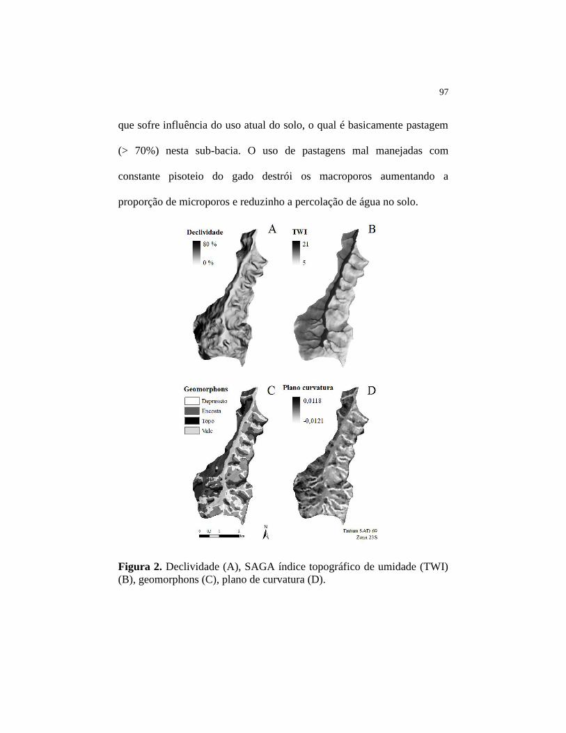
97
que sofre influência do uso atual do solo, o qual é basicamente pastagem
(> 70%) nesta sub-bacia. O uso de pastagens mal manejadas com
constante pisoteio do gado destrói os macroporos aumentando a
proporção de microporos e reduzinho a percolação de água no solo.
Figura 2. Declividade (A), SAGA índice topográfico de umidade (TWI)
(B), geomorphons (C), plano de curvatura (D).

98
Figura 3. Condutividade hidráulica do solo saturado (Ksat) determinada
pelo método GEOM (A), Ksat determinada pelo método AT (B),
profundidade do solum (PROF) determinada pelo método GEOM (C) e
PROF determinada pelo método TA (D).
Devido à melhor precisão do método GEOM para predizer os
atributos do solo estudados, este também foi o método escolhido para
gerar o mapa de solos para a sub-bacia (Figura 4). De acordo com os

99
resultados a maior parte da sub-bacia (55%) é composta por Cambissolos.
Os Cambissolos têm sua ocorrência vinculada às áreas de declives
acentuados que proporcionam deflúvio severo e dificuldades de
mecanização. Dessa forma, tornam-se vulneráveis ao processo erosivo
sendo restritos a cultivos anuais que requerem maiores intervenções e
sendo preferível para o uso com pastagens, reflorestamentos e algumas
culturas permanentes protetoras do solo, desde que adequadamente
manejadas, utilizando práticas especiais de conservação do solo, uma vez
que, mesmo sob este tipo de vegetação, esses solos são suscetíveis ao
processo erosivo (Silva et al., 2013).
O segundo solo de maior ocorrência na sub-bacia é o Argissolo, o
qual é mais desenvolvido, mais profundo e também mais resistente à
erosão que os Cambissolos. Entretanto, apesar de mais resistente à erosão
o Argissolo ainda é muito susceptível a perdas de solo devido ao
gradiente textural entre o horizonte A e B levando estes solos a
degradação quando práticas conservacionistas e cobertura do solo são
ausentes.
Associado ao Argissolo e Cambissolos temos o Neossolo Litólico
que apresenta afloramentos de rochas impossibilitando que seja cultivado.
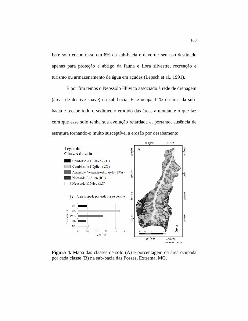
100
Este solo encontra-se em 8% da sub-bacia e deve ter seu uso destinado
apenas para proteção e abrigo da fauna e flora silvestre, recreação e
turismo ou armazenamento de água em açudes (Lepsch et al., 1991).
E por fim temos o Neossolo Flúvico associado à rede de drenagem
(áreas de declive suave) da sub-bacia. Este ocupa 11% da área da sub-
bacia e recebe todo o sedimento erodido das áreas a montante o que faz
com que esse solo tenha sua evolução retardada e, portanto, ausência de
estrutura tornando-o muito susceptível a erosão por desabamento.
Figura 4. Mapa das classes de solo (A) e porcentagem da área ocupada
por cada classe (B) na sub-bacia das Posses, Extrema, MG.

101
A análise da vulnerabilidade do solo ao escoamento superficial
mensal revelou que os meses mais críticos são de novembro a março
(Figura 5). De acordo com o índice utilizado neste trabalho para avaliar o
escoamento quando o grau de saturação do solo é significante o risco de
erosão e transporte de sedimentos é alto (Oliveira, 2011). Nos meses de
dezembro e janeiro praticamente toda a sub-bacia está sob risco de
erosão, exceto os topos de morro. Aliás, os topos de morros não
apresentaram vulnerabilidade ao escoamento e risco de erosão em
nenhum dos meses analisados indicando que estas áreas são importantes
na infiltração de água e abastecimento do lençol freático.
Durante os meses de maio a agosto, o qual é o período de seca na
região com precipitação média mensal inferior a 50 mm é possível
observar que a saturação do solo é significante somente próximo à rede de
drenagem. Isto evidencia a importância das APPs nas margens do ribeirão
das Posses, pois o risco de erosão nessas áreas é evidente durante todos os
meses do ano necessitando que o solo esteja protegido permanentemente
evitando que as erosões nas bordas do rio aumentem o assoreamento dos
mananciais interferindo no abastecimento de água.

102
Os meses de abril e setembro são os meses de transição entre o
período de seca e o período de chuva na sub-bacia e apresentaram maior
vulnerabilidade nas áreas de maiores declives principalmente nas áreas de
cabeceira.
Figura 5. Vulnerabilidade mensal ao escoamento superficial e
precipitação media mensal para a sub-bacia das Posses, MG.
Na Tabela 1 encontram-se as porcentagens da área da sub-bacia
das Posses vulneráveis ao escoamento superficial de acordo com o uso
atual do solo. O mês mais crítico ao escoamento superficial que é o mês
de janeiro apresentou maior parte das áreas de agricultura com risco
insignificante de ocorrer escoamento, aproximadamente metade das áreas
103
de eucaliptos, pastagem e floresta nativa com risco significante e a outra
metade com risco insignificante e cerca de 70% da APP com risco
significante de escoamento. Isso mostra que as APPs implantadas pelo
Conservador de Águas são muito úteis na conservação do solo, pois estão
alocados na sub-bacia em áreas críticas a erosão durante todo o ano.
Em geral, nos meses de maior vulnerabilidade ao escoamento e
erosão (novembro a março) os usos pastagem e APP foram que se
encontram nas áreas de maiores risco. As pastagens quando bem
manejadas auxiliam na redução da erosão hídrica. Entretanto, de acordo
com Oliveira et al. (2008), as pastagens na sub-bacia das Posses se
encontram em avançado estágio de degradação necessitando de um plano
de manejo adequado que garanta o uso sustentável dessas pastagens,
principalmente, por elas se encontrarem nas áreas mais susceptíveis ao
escoamento superficial e erosão do solo.

104
Tabela 1. Porcentagem da área da sub-bacia das Posses vulnerável ao
escoamento superficial de acordo com o uso atual do solo.
Mês Escoamento
superficial Agric.
(1) Euc.
(2) Past.
(3)
Floresta
Nativa APP
(4)
Jan. Insignificante 73 55 48 50 32
Significante 27 45 52 50 68
Fev. Insignificante 92 81 75 77 58
Significante 8 19 25 23 42
Mar. Insignificante 89 77 70 71 51
Significante 11 23 30 29 49
Abr. Insignificante 96 86 83 83 67
Significante 4 14 17 17 33
Mai. Insignificante 100 94 96 95 87
Significante 0 6 4 5 13
Jun. Insignificante 100 91 91 90 79
Significante 0 9 9 10 21
Jul. Insignificante 100 91 93 91 81
Significante 0 9 7 9 19
Ago. Insignificante 100 93 95 94 85
Significante 0 7 5 6 15
Set. Insignificante 98 89 87 86 72
Significante 2 11 13 14 28
Out. Insignificante 94 84 80 80 64
Significante 6 16 20 20 36
Nov. Insignificante 90 78 71 73 53
Significante 10 22 29 27 47
Dez. Insignificante 85 70 63 65 45
Significante 15 30 37 35 55 (1)
Agricultura, (2)
Eucalipto, (3)
Pastagem, (4)
Área de preservação
permanente.
Conclusões
1. Os dois atributos do solo analisados condutividade hidráulica do solo
saturado (Ksat) e profundidade do solum (PROF) tiveram melhor

105
precisão quando os atributos do terreno declividade, plano de
curvatura, SAGA índice topográfico de umidade, elevação e
geomorphons foram combinados.
2. Devido à melhor precisão do método GEOM para predizer os
atributos do solo estudados, este também foi o método escolhido para
gerar o mapa de solos para a sub-bacia e esta apresentou: 55% da
área com Cambissolos (Cambissolo Háplico e Húmico), 26% de
Argissolo Vermelho-Amarelo, 8% de Neossolo Litólico e 11% com
Neossolo Flúvico.
3. Os meses de maior vulnerabilidade ao escoamento superficial foram
os meses de novembro a março, abril e setembro apresentaram maior
risco na área de cabeceira enquanto que os meses de baixa
precipitação (maio a agosto) o risco de escoamento superficial e
erosão se deram próximo à rede de drenagem.
4. Nos meses de maior vulnerabilidade ao escoamento e erosão
(novembro a março) os usos pastagem e APP foram que se
encontram nas áreas de maiores risco devendo ser mantidas as APPs
e conservadas as pastagens.

106
Agradecimentos
À Prefeitura Municipal de Extrema, em nome do Diretor do
Departamento de Meio Ambiente, Paulo Henrique Pereira, pelo apoio na
obtenção dos dados, ao Conselho Nacional de Desenvolvimento
Científico e Tecnológico – CNPq Brasil (Processos no
471522/2012-0 e
201987/2012-0);
À Coordenação de Aperfeiçoamento de Pessoal de Nível Superior
– CAPES Brasil e à Fundação de Amparo à Pesquisa do Estado de Minas
Gerais – FAPEMIG (Processos no CAG-APQ-01423-11 e CAG-PPM-
00422-13), pelo suporte financeiro.
Referências
AGÊNCIA NACIONAL DE ÁGUAS. Programa produtor de água
superintendência de usos múltiplos. Brasília: Ministério do Meio Ambiente,
2008. 60p.
ASHTEKAR, J. M.; OWENS, P. R. Remembering Knowledge: An Expert
Knowledge Based Approach to Digital Soil Mapping. Soil Horizons, v. 54, n. 5,
p. 1-6, Sep. 2013. DOI: 10.2136/sh13-01-0007.
BEVEN, K. J.; KIRKBY, M. J. A physically based, variable contributing area
model of basin hydrology / Un modèle à base physique de zone d’appel variable
de l'hydrologie du bassin versant. Hydrological Sciences Bulletin, v. 24, n. 1, p.
43–69, 1979. DOI:10.1080/02626667909491834
BOER, M.; DEL BARRIO, G.; PUIGDEFÁBRES, J. Mapping soil depth
classes in dry Mediterranean areas using terrain attributes derived from a digital
elevation model. Geoderma, v. 72, n.1-2, p. 99–118, 1996. DOI:10.1016/0016-
7061(96)00024-9

107
DIETRICH, W.; WILSON, C. Analysis of erosion thresholds, channel networks,
and landscape morphology using a digital terrain model. The Journal of
Geology, v. 101, n. 2, p. 259–278, 1993.
DUNNE, T.; LEOPOLD, L. B. Water in environment planning. São
Francisco: Freeman, 1978. 818p.
JASIEWICZ, J.; STEPINSKI, T. F. Geomorphons — a pattern recognition
approach to classification and mapping of landforms. Geomorphology, v. 182,
p. 147–156, 2013. DOI:10.1016/j.geomorph.2012.11.005
LEPSCH, I. F. BELLINAZI JR., R.; BERTOLINI, D.; ESPÍNDOLA, C.R.
Manual para levantamento utilitário do meio físico e classificação de terras
no sistema de capacidade de uso: 4ª aproximação. Campinas: Sociedade
Brasileira de Ciência do Solo, 1991. 175p.
LIAO, W.-H. Region Description Using Extended Local Ternary Patterns.
In: 2010 20th International Conference on Pattern Recognition, p. 1003–1006,
2010. DOI:10.1109/ICPR.2010.251
LIMA, J. M.; CURI, N.; RESENDE, M.; SANTANA, D. P. Dispersão do
material de solo em água para avaliação indireta da erodivilidade da Latossolos.
Revista Brasileira de Ciência do Solo, v. 14, n. 1, p. 85-90, 1990.
McBRATNEY, A., MENDONÇA-SANTOS, M.; MINASNY, B. On digital soil
mapping. Geoderma, v. 117, n. 1-2, p.3–52, 2013. DOI:10.1016/S0016-
7061(03)00223-4
MENEZES, M. D. Levantamento pedológico de hortos florestais e
mapeamento digital de atributos físicos do solo para estudos hidrológicos.
2011. 225 p. Tese (Doutorado em Ciência do Solo) – Universidade Federal de
Lavras, Lavras, Minas Gerais, 2011.
MONTGOMERY, D. R.; DIETRICH, W. E. A physically based model for the
topographic control on shallow landsliding. Water Resources Research, v. 30,
n. 4, p. 1153–1171, 1994. DOI:10.1029/93WR02979
MOORE, I.D.; GESSLER, P.E.; NIELSEN, G. A.; PETERSON, G. A. Soil
Attribute Prediction Using Terrain Analysis. Soil Science Society of America
Journal, v. 57, n. 2, p. 443-452, 1993.

108
MOTAGHIAN, H. R.; MOHAMMADI, J. Spatial Estimation of Saturated
Hydraulic Conductivity from Terrain Attributes Using Regression, Kriging, and
Artificial Neural Networks. Pedosphere, v. 21, n. 2, p. 170–177, 2011.
DOI:10.1016/S1002-0160(11)60115-X
O’LOUGHLIN, E. M. Prediction of Surface Saturation Zones in Natural
Catchments by Topographic Analysis. Water Resources Research, v. 22, n. 5,
p. 794–804, 1986. DOI:10.1029/WR022i005p00794
ODEH, I.; McBRATNEY, A.; CHITTLEBOROUGH, D. Further results on
prediction of soil properties from terrain attributes: heterotopic cokriging and
regression-kriging. Geoderma, v. 67, n. 1995, p. 215–226, 1995.
OLIVEIRA, A. H. Erosão hídrica e seus componentes na sub-bacia
hidrográfica do Horto Florestal Terra Dura, Eldorado do Sul (RS). 2011.
181p. Tese (Doutorado em Ciência do Solo) – Universidade Federal de Lavras,
Lavras.
OLIVEIRA, A. H.; LIMA, G.C.; SILVA, M.L.N.; FREITAS, D.A.F; SILVA,
M.A.; PEREIRA, P.H.; SANTOS, D.G.; VEIGA, F. Implantação de práticas
conservacionistas em áreas agrícolas e estradas, objetivando a recarga de água
na sub-bacia das Posses, município de Extrema, MG. In: CONGRESSO DE
PÓS-GRADUAÇÃO DA UFLA, I ENCONTRO DE ENGENHARIA DE
SISTEMAS E IV WORKSHOP DE LASER E ÓPTCA NA AGRICULTURA,
17. , 2008, Lavras. Anais. Lavras: UFLA, 2008. p.354-359.
OLIVEIRA, A. H.; SILVA, M. L. N.; CURI, N.; KLINKE NETO, G.; SILVA,
M. A; ARAÚJO, E. F. Consistência hidrológica de modelos digitais de elevação
(MDE) para definição da rede de drenagem na sub-bacia do horto florestal Terra
Dura, Eldorado do Sul, RS. Revista Brasileira de Ciência do Solo, v. 36, n.4,
p.1259–1268, 2012. DOI:10.1590/S0100-06832012000400020
SILVA, M. A.; FREITAS, D. A. F.; SILVA, M. L. N.; OLIVEIRA, A. H.;
LIMA, G. C.; CURI, N. Sistema de informações geográficas no planejamento de
uso do solo. Revista Brasileira de Ciências Agrárias, v. 8, n. 2, p. 316–323,
2013. DOI:10.5039/agraria.v8i2a2289
TARBOTON, D. G. A new method for the determination of flow directions and
upslope areas in grid digital elevation models. Water Resources Research, v.
33, n. 2, p. 309–319, 1997. DOI:10.1029/96WR03137

109
WINZELER, H. E.; OWENS, P. R.; JOERN, B. C.; CAMBERATO, J. J.; LEE,
B. D.; ANDERSON, D. E.; SMITH, D. R. Potassium Fertility and Terrain
Attributes in a Fragiudalf Drainage Catena. Soil Science Society of America
Journal, v. 72, n. 5, p. 1311-1320, 2008. DOI:10.2136/sssaj2007.0382
ZHU, A. X.; HUDSON, B.; BURT, J.; LUBICH, K.; SIMONSON, D. Soil
Mapping Using GIS, Expert Knowledge, and Fuzzy Logic. Soil Science Society
of America Journal, v. 65, n. 5, p. 1463–1472, 2001.
DOI:10.2136/sssaj2001.6551463x
ZHU, A.; BAND, L. A knowledge-based approach to data integration for soil
mapping. Canadian Journal of Remote Sensing, v. 20, n.4, p. 408–418, 1994.
ZHU, A.-X. A similarity model for representing soil spatial information.
Geoderma, v. 77, n. 2-4, p. 217–242, 1997. DOI:10.1016/S0016-
7061(97)00023-2
ZHU, A.-X.; BAND, L. E.; DUTTON, B.; NIMLOS, T. J. Automated soil
inference under fuzzy logic. Ecological Modelling, v. 90, n. 2, p. 123–145,
1996. DOI:10.1016/0304-3800(95)00161-1
ZHU, A.-X.; BAND, L.; VERTESSY, R.; DUTTON, B. Derivation of Soil
Properties Using a Soil Land Inference Model (SoLIM). Soil Science Society of
America Journal, v. 61, n. 2, p. 523–533, 1997.
DOI:10.2136/sssaj1997.03615995006100020022x
ZHU, A.-X.; QI, F.; MOORE, A.; BURT, J. E. Prediction of soil properties
using fuzzy membership values. Geoderma, v. 158, n. 3-4, p. 199–206, 2010.
DOI:10.1016/j.geoderma.2010.05.001
ZHU, Q.; LIN, H. S. Comparing Ordinary Kriging and Regression Kriging for
Soil Properties in Contrasting Landscapes. Pedosphere, v. 20, n. 5, p. 594–606,
2010. DOI:10.1016/S1002-0160(10)60049-5