Laboratorio Nacional de Computacao Cientıfica

Programa de Pos-Graduacao em Modelagem Computacional

Analise da Implementacao da Porta Toffoli em Sistemas

com Imperfeicoes

Por

Jalil Khatibi Moqadam

PETROPOLIS, RJ - BRASIL

JANEIRO DE 2014

ANALISE DA IMPLEMENTACAO DA PORTA TOFFOLI EM

SISTEMAS COM IMPERFEICOES

Jalil Khatibi Moqadam

TESE SUBMETIDA AO CORPO DOCENTE DO LABORATORIO NA-

CIONAL DE COMPUTACAO CIENTIFICA COMO PARTE DOS REQUISITOS

NECESSARIOS PARA A OBTENCAO DO GRAU DE DOUTOR EM CIENCIAS

EM MODELAGEM COMPUTACIONAL

Aprovada por:

Prof. Renato Portugal, D.Sc

(Presidente)

Prof. Paulo Cesar Marques Vieira, D.Sc.

Prof. Marcos Cesar de Oliveira, D.Sc.

Prof. Reinaldo Oliveira Vianna, D.Sc.

PETROPOLIS, RJ - BRASILJANEIRO DE 2014

Khatibi Moqadam, Jalil

K45a Analise da implementacao da porta Toffoli em sistemas com imperfeicoes

/ Jalil Khatibi Moqadam. Petropolis, RJ. : Laboratorio Nacional de Com-

putacao Cientıfica, 2014.

xii, 69 p. : il.; 29 cm

Orientadore(s): Renato Portugal , Nami Fux Svaiter e Gilberto Oliveira Correa

Tese (D.Sc.) – Laboratorio Nacional de Computacao Cientıfica, 2014.

1. Computadores quanticos 2. Computacao quantica 3. Teoria do con-

trole em fısica matematica 4. Ruıdo quantico. I. Portugal, Renato. II.

LNCC/MCT. III. Tıtulo.

CDD 004.1

“There is no such thing as teaching

without research and research

without teaching.”

(Paulo Freire)

iv

To my wife

for her love and patience

v

Acknowledgment

I would like to express my thanks to Dr. Renato Portugal not only for his

supervising during the preparation of this thesis but also for helping me to come

to Brazil that led to a quite different invaluable experience in my life.

I also want to give my thanks to Dr. Gilberto Correa and Dr. Nami Svaiter

for their contribution to this work.

I wish to thank Dr. Paulo Cesar and Dr. Paulo Esquef from whom I learned

a lot during these years.

I acknowledge Conselho Nacional de Desenvolvimento Cientıfico e Tecnologico

(CNPq) for the PhD scholarship.

vi

Resumo da Tese apresentada ao LNCC/MCT como parte dos requisitos necessarios

para a obtencao do grau de Doutor em Ciencias (D.Sc.)

ANALISE DA IMPLEMENTACAO DA PORTA TOFFOLI EM

SISTEMAS COM IMPERFEICOES

Jalil Khatibi Moqadam

Janeiro , 2014

Orientador: Renato Portugal, D.Sc

Co-advisors: Nami Fux Svaiter, D.Sc.

Gilberto Oliveira Correa, Ph.D

Neste trabalho, o desempenho da porta Toffoli sob a influencia de imper-

feicoes e estudada. Depois de dar uma breve introducao a computacao quantica

e teoria de controle quantico, os qubits supercondutores de tipo de carga e seus

acoplamentos a um ressonador da linha de transmissao sao discutidos. Em seguida,

a execucao da porta Toffoli numa cadeia de tres qubits supercondutores de tipo

transmon, utilizando metodos de controle quantico, e revisada. Tendo estabele-

cido a porta, o ruıdo e introduzido nas interacoes entre os qubits. As constantes de

acoplamento, entao, nao ficam fixas, flutuam em torno de valores medios e obede-

cem a algumas funcoes de densidade de probabilidade conhecidas que caracterizam

o caso da imperfeicao dinamica. O caso da imperfeicao estatica no qual os valores

das constantes de acoplamento nao sao conhecidas com precisao e tambem consi-

derado. Finalmente, uma porta mais robusta e projetada com uma modificacao do

problema de otimizacao quantico usando uma fidelidade media ponderada como

funcional objetivo.

vii

Abstract of Thesis presented to LNCC/MCT as a partial fulfillment of the

requirements for the degree of Doctor of Sciences (D.Sc.)

ANALYZING THE IMPLEMENTATION OF THE TOFFOLI GATE

IN SYSTEMS WITH IMPERFECTIONS

Jalil Khatibi Moqadam

January, 2014

Advisor: Renato Portugal, D.Sc

Co-advisors: Nami Fux Svaiter, D.Sc.

Gilberto Oliveira Correa, Ph.D

In this thesis, the performance of the Toffoli gate under the influence of im-

perfections is studied. After giving a brief introduction to quantum computing

and quantum control theory, superconducting charge qubits and their couplings

to the transmission line resonator are discussed. Then, the implementation of the

Toffoli gate in a chain of three superconducting transmon qubits, using quantum

control methods, is reviewed. Having established the gate, the noise is introduced

in the interqubits interactions. The coupling constants are then no longer fixed, in-

stead, they fluctuate around average values obeying some given probability density

functions characterizing the dynamical-imperfection case. The static-imperfection

case in which the values of the coupling constants are not exactly known is also

considered. Finally, a more robust gate is designed by modifying the quantum

optimization problem using some weighted average fidelity as the objective func-

tional.

viii

Contents

1 Introduction 1

2 Quantum Computing and Quantum Control Theory 6

2.1 Quantum computing . . . . . . . . . . . . . . . . . . . . . . . . . . 6

2.1.1 Entanglement . . . . . . . . . . . . . . . . . . . . . . . . . . 10

2.1.2 Physical Implementation of Quantum Gates . . . . . . . . . 11

2.2 Quantum Control Theory . . . . . . . . . . . . . . . . . . . . . . . 13

2.2.1 Controllability . . . . . . . . . . . . . . . . . . . . . . . . . . 14

2.2.2 Optimal Control . . . . . . . . . . . . . . . . . . . . . . . . 17

2.2.3 Bilinear Model . . . . . . . . . . . . . . . . . . . . . . . . . 18

3 Superconducting Qubits and Circuit Quantum Electrodynamics 20

3.1 Josephson Junction . . . . . . . . . . . . . . . . . . . . . . . . . . . 21

3.2 Superconducting Charge Qubits . . . . . . . . . . . . . . . . . . . . 23

3.2.1 Transmon Qubit . . . . . . . . . . . . . . . . . . . . . . . . 27

3.3 Circuit Quantum Electrodynamics . . . . . . . . . . . . . . . . . . . 29

4 Implementation of the Toffoli Gate in Systems with Imperfections 35

4.1 Review of the Implementation of the Toffoli Gate in the Perfect

System . . . . . . . . . . . . . . . . . . . . . . . . . . . . . . . . . . 35

4.2 Noise Model . . . . . . . . . . . . . . . . . . . . . . . . . . . . . . . 38

4.3 Analyzing the Dynamical Imperfections . . . . . . . . . . . . . . . . 40

4.4 Analyzing the Static Imperfection . . . . . . . . . . . . . . . . . . . 45

ix

4.5 Summary and Conclusions . . . . . . . . . . . . . . . . . . . . . . . 46

5 Improving the Gate Fidelity in Systems with Imperfections 52

5.1 Optimizing the Weighted Average Fidelity . . . . . . . . . . . . . . 52

5.2 Performance of the New Optimized Sets of Control Fields . . . . . . 55

5.3 Stable Toffoli Gate under the Influence of Static Imperfection . . . 56

5.4 Summary and Conclusions . . . . . . . . . . . . . . . . . . . . . . . 57

6 Summary, Conclusions and Future Works 61

Bibliography 65

x

List of Figures

Figure

3.1 The Josephson junction device . . . . . . . . . . . . . . . . . . . . . 22

3.2 The Josephson junction circuit symbol . . . . . . . . . . . . . . . . 23

3.3 The superconducting charge qubit . . . . . . . . . . . . . . . . . . . 24

3.4 The energy levels of the superconducting charge qubit . . . . . . . . 25

3.5 The superconducting charge qubit with tunable Josephson energy . 26

3.6 The energy levels of the superconducting charge qubit for different

values of EJ/EC . . . . . . . . . . . . . . . . . . . . . . . . . . . . . 28

3.7 The transmon qubit circuit . . . . . . . . . . . . . . . . . . . . . . . 28

3.8 The circuit quantum electrodynamic setup . . . . . . . . . . . . . . 31

4.1 The average fidelity versus standard deviation (single source of noise) 48

4.2 The average fidelity versus standard deviation (three independent

sources of noise) . . . . . . . . . . . . . . . . . . . . . . . . . . . . . 48

4.3 The average fidelity versus standard deviation (six independent sources

of noise) . . . . . . . . . . . . . . . . . . . . . . . . . . . . . . . . . 49

4.4 The average fidelity versus standard deviation at large values of

standard deviation (single source of noise) . . . . . . . . . . . . . . 49

4.5 The average fidelity versus standard deviation at large values of

standard deviation (three independent sources of noise) . . . . . . . 50

4.6 The average fidelity versus standard deviation at large values of

standard deviation (six independent sources of noise) . . . . . . . . 50

4.7 The average fidelity versus half-width in the case of static noise . . 51

xi

5.1 Fidelity versus J/J for different sets of control fields . . . . . . . . . 54

5.2 The average fidelity versus half-width in the case of static noise for

different sets of control fields . . . . . . . . . . . . . . . . . . . . . . 59

5.3 Fidelity versus J/J for the set of control fields that leads to a con-

stant fidelity around the perfect value of the couplings as well as for

two other sets of control fields . . . . . . . . . . . . . . . . . . . . . 60

xii

Chapter 1

Introduction

Physical implementations of quantum information processing are always sub-

jected to various imperfections that decrease the performance of the process. Im-

perfections can be dynamical or static. While in dynamical imperfections the noisy

parameters change their values in time with some frequencies, in static imperfec-

tions the realization of the noise parameters remain constant for a time period

much larger than the time that is required to fulfill the process job.

Dynamical imperfections as a result of system-environment coupling produce

decoherence in the system destroying the benefits of using quantum information.

Static imperfections on the other hand do not introduce decoherence to the system

yet lead to error as well.

Georgeot and Shepelyansky (2000b,a) have already considered a two di-

mensional lattice of qubits with nearest-neighbor interqubit couplings as a stan-

dard generic quantum computer model to incorporate imperfections. This model

shows that, for a system affected by static imperfections, quantum chaos sets in

above a critical interqubit strength and annihilates the quantum computer perfor-

mance (Georgeot and Shepelyansky (2000a)).

Consequently, the entanglement dynamics also exhibit a transition from in-

tegrability to quantum chaos (Montangero et al. (2003); Montangero and Viola

(2006)). However, the entanglement dynamics remain almost unaffected for disor-

ders less than 10% (Tsomokos et al. (2007, 2008)).

1

Facchi et al. (2005) have also used the same model to study the dynamical

imperfections in quantum computers. In this case a characteristic frequency is

associated with the noise that is specifying the rate at which the noise changes.

They have shown that for low frequencies the imperfections can be considered

static, and for sufficiently high frequencies the effect of noise completely disappears.

Implementations of quantum computers specifically require high fidelity quan-

tum gates. There are many measures for the robustness of a quantum gate against

noise (see for example Harrow and Nielsen (2003)). Particularly, one- and two-

qubit quantum gates that are universal for quantum computing have already been

analyzed under the influence of noise (Hu and Das Sarma (2002); Paladino et al.

(2011); Green et al. (2012); Bogdanov et al. (2013)).

The standard way of implementation of the multiqubit gates is to decompose

them into a sequence of single- and two-qubit gates (Barenco et al. (1995)). How-

ever, the implementation of multi-qubit gates using such decompositions in terms

of a universal gate set may not be efficient because the implementation time may

exceed the decoherence time.

Another approach to implement multiqubit gate is to implement them di-

rectly without using the decomposition method. The Toffoli gate, a three-qubit

gate with central role in quantum information processing, has been recently im-

plemented with less resources and moderate fidelities (Monz et al. (2009); Fedorov

et al. (2011); Reed et al. (2012a)). However, new proposals have been suggested

to realize the Toffoli gate with fidelities above 99% (Stojanovic et al. (2012); Chen

et al. (2012)).

It is possible to use quantum control methods to design a set of microwave

pulses to realize the Toffoli gate in a chain of three superconducting qubits which

are embedded in circuit quantum electrodynamics (circuit QED) setup.

Superconducting qubits are promising candidates in constructing quantum

networks to perform quantum information processing tasks. They are macroscopic

prototypes of qubits which are based on Josephson tunnel junction and proved to

2

have quantum properties like atoms (Clarke and Wilhelm (2008); You and Nori

(2011)). Superconducting qubits are coupled to microwave photons within cir-

cuit QED setup which is the on-chip implementation of the cavity quantum elec-

trodynamics (cavity QED). It consists of a transmission line resonator playing the

role of the cavity and a superconducting qubit serving as the artificial atom. The

Jaynes-Cummings model describes the interaction between the photon and the

qubit, when the so called rotating wave approximation is applicable (Blais et al.

(2004); Schoelkopf et al. (2008)). The control and readout of the qubit state can

be effectively performed using external wave generators.

The coupling between the qubits within a circuit QED is mediated by virtual

exchange of photons with the cavity in the large detuning dispersive regime. In this

regime, an effective qubit-qubit interaction of isotropic XY type appears when the

rotating wave approximation is applicable (Blais et al. (2004, 2007); Majer et al.

(2007)). Various two- and three-qubit quantum information processing tasks have

already been performed with moderate fidelities using such coupling between the

qubits (DiCarlo et al. (2009, 2010); Fedorov et al. (2012); Reed et al. (2012b)).

Actually in a circuit QED setup, Stojanovic et al. (2012) design a sequence

of microwave pulses that realizes the Toffoli gate with a fidelity above 99% in a

time about 140 ns that is fast enough because the decoherence time T2 in such

systems is 10 to 20 µs.

Having design such multiqubit gates, it is crucial to analyze their efficiency

under the influence of noise and possibly to improve their performance.

A bilinear Hamiltonian with XY -type Heisenberg chain for the system and

Zeeman-like term for the control part is considered as the quantum control system

to implement the Toffoli gate. Both parts in the Hamiltonian are subjected to noise.

The effect of noise on the control fields has already been considered (Stojanovic

et al. (2012); Heule et al. (2010, 2011)) showing that the gate is more robust

when the single control pulse duration is reduced. Actually, for a fixed gate time,

increasing the noise has less of an effect on the average fidelity of the gate with

3

higher number of control pulses. However, the system Hamiltonian is also subjected

to imperfections when the interqubit couplings are affected by the noise.

In this thesis, we consider the Toffoli gate that is proposed by Stojanovic

et al. (2012) and study the performance of the gate when the interqubit couplings

are noisy. We consider the fidelity of the Toffoli gate under the influence of both

the dynamical and the static imperfections. We also propose a method to improve

the performance of the gate in the presence of noise.

In chapter 2 the ideas of quantum computing and quantum control theory

are explained. After briefly reviewing the postulates of quantum mechanics, the

quantum mechanical counterpart of the classical bit, the quantum bit (qubit) is

described and finally the universal set of gates are introduced. The entangled

and separable states are defined and the physical implementation of the quantum

gates are presented thereafter. The chapter in continued with giving the ideas of

quantum control theory and then the various forms of controllability explained.

Some theorems that help to verifying the controllability of the quantum systems

is pointed out. The chapter is ended with an explanation on the quantum optimal

control theory and the bilinear model.

Chapter 3 is devoted to explaining superconducting qubits and circuit QED

setup. The chapter starts with describing the Josephson junction that consists

the basis of the superconducting qubits. The Hamiltonian of the single Josephson

junction charge qubit is then presented and the ideas of qubits with two and three

junctions are explained. As a charge qubit that is more resisted to the charge noise

the transmon qubit is then described. Finally, the coupling of the superconducting

qubits to a transmission line resonator are considered. It is described how to control

a single qubit embedded in the circuit QED. The Hamiltonian of several qubits

coupled to a single transmission line is also presented and the effective interaction

between the qubits in the large dispersive regime is studied.

Having presented the required basis in chapters 2 and 3, analyzing the Tof-

foli gate in the presence of noise is discussed in chapter 4. The first part of the

4

chapter is devoted to briefly describing how the Toffoli gate is realized in a chain of

superconducting qubits embedded in circuit QED setup when everything is ideal.

To introduce imperfection to the system a noise model with a triangular form for

the autocorrelation function and consequently a square sinc form for the power

spectral density is described. After that the effect of the dynamical noise which

is characterized by the noise frequency is studied. Actually, the behavior of the

fidelity of the Toffoli gate is considered under the influence of imperfections with

different noise frequencies and different noise standard deviations values. The chap-

ter is ended with an explanation of the effects of the static noise which corresponds

to a fixed noise in the system.

In chapter 5 it is investigated how to improve the fidelity when the system

is affected by the static noise. Using optimal control techniques, two new set of

control fields are obtained and their performance is analyzed under the influence of

the noise that prove the enhanced fidelity. At the end special set of control fields

is obtained that are quite independent from the noise in the interqubit couplings.

The conclusion and future works is presented in chapter 6.

5

Chapter 2

Quantum Computing and Quantum

Control Theory

In this chapter the bases of quantum computing and quantum control theory

are briefly reviewed. The postulates of quantum mechanics, the ideas of qubit

and quantum gates are described in section 2.1. The definition of entanglement is

then given and finally the physical implementation of quantum gates are described.

Section 2.2 is devoted to explaining the ideas of quantum control theory. Various

forms of controllability are described and some theorems are given thereafter that

help to verify the controllability of the quantum systems. The section is finished

with explaining the optimal control methods in bilinear systems.

The postulates of quantum mechanics that are described in this chapter as

well as the ideas of quantum computing is mainly based on Nielsen and Chuang

(2010). The definitions of entangled and separable states are extracted from the

reference Vedral (2006). In writing the section of physical implementation of quan-

tum gate Le Bellac (2006) and Lambropoulos and Petrosyan (2007) have been used.

The quantum control section is mainly based on d’Alessandro (2008) and Machnes

et al. (2011).

2.1 Quantum computing

In this section, first the general framework of quantum mechanics is reviewed

and then the ideas of quantum information theory are briefly described.

6

The state space of a quantum system is described by a Hilbert space H. The

state of the system is completely described by a unit vector |ψ〉 in the corresponding

Hilbert space. The time evolution of the state of a closed quantum system is

described by the Schrodinger equation

d

dtψ(t) = − i

~Hψ(t), (2.1)

where H is the Hamiltonian of the system, ~ is the Planck’s constant and i =√−1

is the imaginary unit.

Considering that the Hamiltonian of the system is a Hermitian operator, the

time evolution of a closed quantum system is described by a unitary transformation.

In the case of time-independent Hamiltonian, the Eq. (2.1) has the solution

|ψ(t)〉 = U(t)|ψ(0)〉; U(t) = e−i~Ht, (2.2)

where |ψ(0)〉 is the state of the system at t = 0.

Having specified the state of the system and its evolution, the next step is to

measure the system. Quantum measurements are described by a collection Mm

of positive operators acting on the state space of the system being measured. The

operators Mm satisfy the completeness equation

∑m

M †mMm = IH,

where the index m refers to the measurement outcomes that may occur in the

experiment and † represents the conjugate transpose. If the state of the quan-

tum system is |ψ〉 immediately before the measurement, then the probability of

occurrence the result m is given by

p(m) = 〈ψ|M †mMm|ψ〉,

7

and the state of the system after the measurement is

Mm|ψ〉√p(m)

.

Here, the product 〈 . | . 〉 : H ×H → C is the corresponding Hilbert space inner

product.

The last point about the quantum systems which must be mentioned is the

way that the compound systems are described. The state space of a composite

quantum system is the tensor product of the state spaces of the component systems.

The state of the system is given by the tensor product of the states of the individual

subsystems.

The above statements are the postulates of quantum mechanics upon which

the theory is constructed. However, the state of a physical system is often not

perfectly determined. It is only known that the state of the system belongs to the

ensemble

|ψ1〉, |ψ2〉, ..., |ψl〉,

with probabilities

p1, p2, ..., pl,∑j

pj = 1.

In this case, the density operator ρ, defined by

ρ =∑l

|ψj〉〈ψj|, (2.3)

is introduced. The density operator ρ is a positive operator with unit trace. The

previous postulates can also be formulated in terms of the density operator to de-

scribe the ensembles. Such a formulation is mathematically equivalent to the state

vector approach, but provides a more convenient way for dealing with ensembles.

With the above background on quantum mechanics the ideas of quantum

information theory are described in the next paragraphs.

Quantum information theory is the generalization of classical information

8

theory to the quantum world. Basically, it deals with the use of quantum systems

to store information, which is then processed by quantum dynamical laws.

In this thesis, only finite dimensional quantum systems are considered hence

the corresponding Hilbert space is always a complex vector space equipped with

the usual inner product. The quantum counterpart of the bit in the classical

information theory is the qubit (quantum bit) that is a two-level quantum system,

whose state is given by

|ψ〉 = α|0〉+ β|1〉, |α|2 + |β|2 = 1, α, β ∈ C (2.4)

belonging to H = (C2, 〈. , .〉), being |0〉, |1〉 a basis for the Hilbert space H.

A qubit can assume any of a continuum of states given by the linear super-

position (2.4) suggesting an infinite information content. However, this is not the

case since the result of the measurement of the qubit is restricted to |0〉 and |1〉

with the corresponding probabilities |α|2 and |β|2.

The quantum counterparts of logical gates in classical computing are unitary

operators. Universal gates in quantum computing are those unitary operators from

which any other unitary operator over n qubits, U ∈ U(2n), can be constructed.

It can be proved that the collection of single-qubit gates

U(θ, φ) =

cos θ ieiφ sin θ

ie−iφ sin θ cos θ

, θ, φ ∈ R, (2.5)

and the two-qubit controlled-Not gate

CNOT =

1 0 0 0

0 1 0 0

0 0 0 1

0 0 1 0

(2.6)

are universal (Barenco et al. (1995)).

9

An important gate that is used in chapter 4 is the three-qubit Toffoli gate

UToff =

1 0 0 0 0 0 0 0

0 1 0 0 0 0 0 0

0 0 1 0 0 0 0 0

0 0 0 1 0 0 0 0

0 0 0 0 1 0 0 0

0 0 0 0 0 1 0 0

0 0 0 0 0 0 0 1

0 0 0 0 0 0 1 0

(2.7)

which belongs to the unitary group U(23). The Toffoli gate can be decomposed

into six CNOT gates and several single-qubit gates (Nielsen and Chuang (2010)).

The basic idea of quantum computation is the application of a sequence

of designed unitary transformations on a collection of qubits that are prepared

in known initial states and performing designed measurements on the final qubit

states (DiVincenzo et al. (2000)).

2.1.1 Entanglement

The tensor product description of the composite systems in quantum me-

chanics makes a departure from the classical realm where the composite systems

are described by the Cartesian product of the individual subsystem states. The

Hilbert space of a quantum n-partite system is given by H = ⊗nj=1Hj, where Hj

are the Hilbert spaces of the individual subsystems and ⊗ is the tensor product

operation. The general state of the system is then written as

|ψ〉 =∑

i1,i2,...in

ci1,i2,...in|i1〉 ⊗ |i2〉 ⊗ ...⊗ |in〉, (2.8)

where |ij〉 correspond to the bases of individual subsystems and ci1,i2,...in ∈ C. The

state (2.8) cannot in general be decomposed as a product of states of individual

10

subsystems

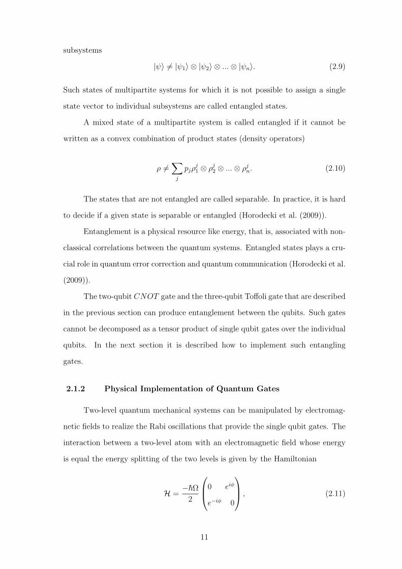
|ψ〉 6= |ψ1〉 ⊗ |ψ2〉 ⊗ ...⊗ |ψn〉. (2.9)

Such states of multipartite systems for which it is not possible to assign a single

state vector to individual subsystems are called entangled states.

A mixed state of a multipartite system is called entangled if it cannot be

written as a convex combination of product states (density operators)

ρ 6=∑j

pjρj1 ⊗ ρj2 ⊗ ...⊗ ρjn. (2.10)

The states that are not entangled are called separable. In practice, it is hard

to decide if a given state is separable or entangled (Horodecki et al. (2009)).

Entanglement is a physical resource like energy, that is, associated with non-

classical correlations between the quantum systems. Entangled states plays a cru-

cial role in quantum error correction and quantum communication (Horodecki et al.

(2009)).

The two-qubit CNOT gate and the three-qubit Toffoli gate that are described

in the previous section can produce entanglement between the qubits. Such gates

cannot be decomposed as a tensor product of single qubit gates over the individual

qubits. In the next section it is described how to implement such entangling

gates.

2.1.2 Physical Implementation of Quantum Gates

Two-level quantum mechanical systems can be manipulated by electromag-

netic fields to realize the Rabi oscillations that provide the single qubit gates. The

interaction between a two-level atom with an electromagnetic field whose energy

is equal the energy splitting of the two levels is given by the Hamiltonian

H =−~Ω

2

0 eiφ

e−iφ 0

, (2.11)

11

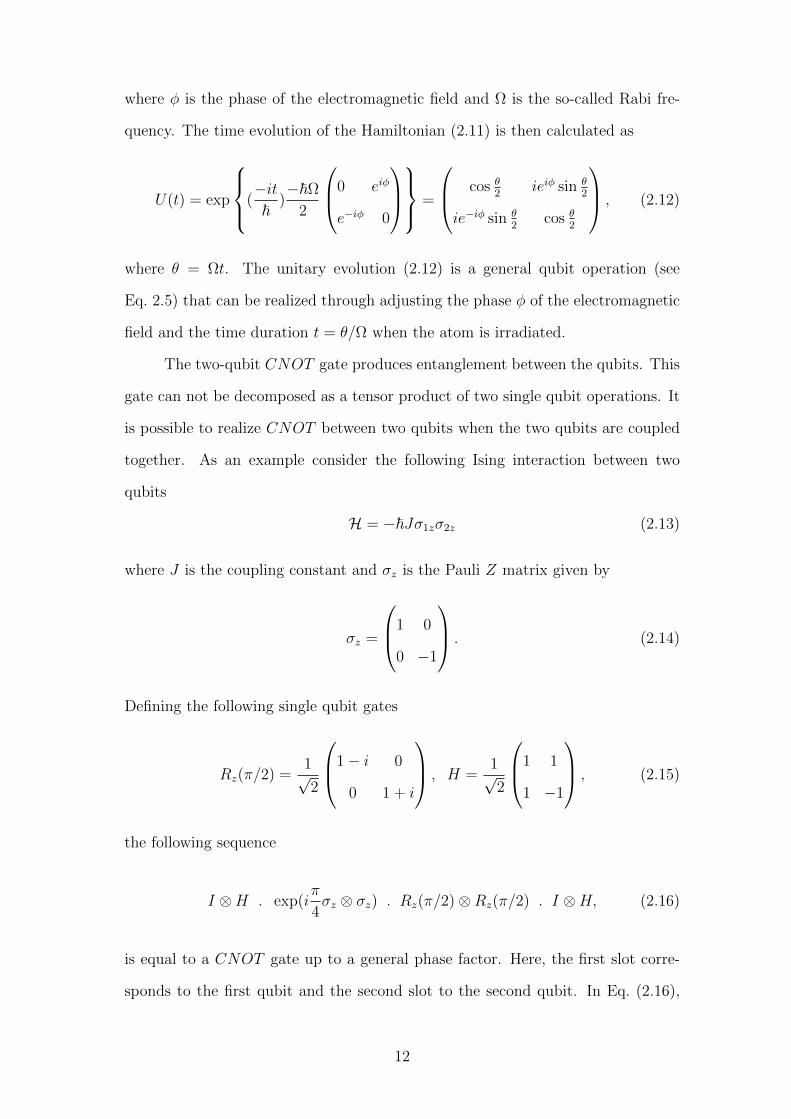
where φ is the phase of the electromagnetic field and Ω is the so-called Rabi fre-

quency. The time evolution of the Hamiltonian (2.11) is then calculated as

U(t) = exp

(−it~

)−~Ω

2

0 eiφ

e−iφ 0

=

cos θ2

ieiφ sin θ2

ie−iφ sin θ2

cos θ2

, (2.12)

where θ = Ωt. The unitary evolution (2.12) is a general qubit operation (see

Eq. 2.5) that can be realized through adjusting the phase φ of the electromagnetic

field and the time duration t = θ/Ω when the atom is irradiated.

The two-qubit CNOT gate produces entanglement between the qubits. This

gate can not be decomposed as a tensor product of two single qubit operations. It

is possible to realize CNOT between two qubits when the two qubits are coupled

together. As an example consider the following Ising interaction between two

qubits

H = −~Jσ1zσ2z (2.13)

where J is the coupling constant and σz is the Pauli Z matrix given by

σz =

1 0

0 −1

. (2.14)

Defining the following single qubit gates

Rz(π/2) =1√2

1− i 0

0 1 + i

, H =1√2

1 1

1 −1

, (2.15)

the following sequence

I ⊗H . exp(iπ

4σz ⊗ σz) . Rz(π/2)⊗Rz(π/2) . I ⊗H, (2.16)

is equal to a CNOT gate up to a general phase factor. Here, the first slot corre-

sponds to the first qubit and the second slot to the second qubit. In Eq. (2.16),

12

the term exp(iπ4σz ⊗ σz) corresponds to the evolution of the Hamiltonian (2.13)

during the time t = π/4J .

Having constructed the general single qubit operations and the CNOT gate,

it is possible theoretically to implement any multiqubit gate. However, the im-

plementation of the multiqubit gates using the standard decompositions in terms

of the universal gates may not be efficient because the implementation time may

exceed the decoherence time. Actually, before finishing the complete sequence

of single and two qubit gates, the qubits interact with the environment and the

quantum information are destroyed.

Another approach to implement multiqubit gate is to implement them di-

rectly by designing a sequence of electromagnetic pulses that affected the qubits

individually and implement the desired gate. In this way, locally manipulating the

qubits leads to generating entanglement that is mediated by the coupling between

the qubits. In chapter 4 it is described how to implement the Toffoli gate using

designed electromagnetic pulses. Such pulse shaping techniques involved quantum

optimal control methods that are described in the next section.

2.2 Quantum Control Theory

In this section the ideas of quantum control theory is described. Pure state

controllability, operator controllability and density matrix controllability are de-

scribed and the corresponding theorems are then explained. Finally, optimal con-

trol theory and the bilinear model that is used for handling the quantum control

problems are described.

Basically, quantum control theory deals with controlling quantum systems

whose behavior is governed by the laws of quantum mechanics. This is not a

trivial task because quantum systems have some unique characteristics such as

entanglement for which there is no classical counterpart.

Like classical systems, it is possible to realize both the open-loop and the

closed-loop control paradigms in quantum systems. In the open-loop quantum

13

control, predetermined controlling actions are applied to the system and no feed-

back is involved. In the closed-loop quantum control in contrast, the controlling

actions depend on the information gained from the system hence it is called feed-

back quantum control (Brif et al. (2010)).

Moreover it is possible to distinguish between two different kinds of closed-

loop quantum control. The distinction originates from the type of information

the controller gains from the system. When the information is classical, some

kind of measurement is involved and the scheme is called measurement feedback

quantum control. It is also possible to use a quantum controller obtaining quantum

information from the system. In this case the system undergoes (nondestructive)

unitary operations. This type of control is called quantum feedback quantum

control or coherent feedback control. It may be mentioned there is no classical

counterpart for this type of quantum control scheme (Brif et al. (2010)).

Two main objectives of quantum control are quantum state engineering and

quantum operator engineering. In quantum state engineering the aim is to steer

the system from an initial state ψi (ρi) to a final state ψf (ρf ). In operator control,

one wish to implement a predetermined operator U irrespective of the initial state

of the system.

Having established the quantum control system, one needs to know about

the controllability of the system. The controllability of the system is associated

with the ability to steer the system from any initial state in the corresponding

Hilbert space to any other state in that space by using the admissible controllers.

In the next section, the state and operator controllability are described in more

details.

2.2.1 Controllability

A fundamental notion in quantum control theory is the controllability of a

given quantum system. Here, some results on the controllability of closed quan-

tum systems with open-loop control are presented. The results for open quantum

14

systems is given thereafter. It is more convenient to set ~ = 1 which is equivalent

to change the units.

Definition 1. (Pure State Controllability) The Schrodinger equation

d

dtψ(t) = −iH(u(t))ψ(t), (2.17)

is pure state controllable if for every pair of initial and final states, ψ0 and ψ1,

there exist control functions u and a time T > 0 such that the solution ψ(t) of

equation (2.17) at time T , with initial condition ψ0, is ψ(T ) = ψ1. Here, u(t) is

assumed to belong to the space of real-valued functions, U .

Definition 2. (Operator Controllability) The Schrodinger operator equation

d

dtU(t) = −iH(u(t))U(t), (2.18)

is operator controllable if for every unitary operator Uf ∈ U(n) with n being the

corresponding dimension of Hilbert space, there exist control functions u and a

time T > 0 such that the solution U(t) of equation (2.18) at time T , with initial

condition U(0) = I, is U(T ) = Uf .

Definition 3. (Density Matrix Controllability) The Liouville equation

d

dtρ(t) = −i[H(u(t)), ρ(t)], (2.19)

is density matrix controllable if, for each pair of unitarily equivalent density matrix

ρ1 and ρ2, there exist control functions u and a time T > 0 such that the solution

ρ(t) of equation (2.19) at time T , with initial condition ρ1, satisfies ρ(T ) = ρ2.

The following theorems give the criteria to verify the controllability of the

equations (2.17−2.19).

Theorem 1. The Schrodinger equation (2.17) is pure state controllable if and

only if the Lie algebra L generated by span−iH(u), u ∈ U satisfies one of the

followings

15

1. L = u(n)

2. L = su(n)

3. L = spaniIn×n ⊕ L

4. L is conjugate to sp(n2)

where n is the dimension of the corresponding Hilbert space, u(n) is the Lie algebra

of anti-Hermitian n × n matrices, su(n) is the Lie algebra of zero trace anti-

Hermitian n × n matrices, sp(n2) is the symplectic Lie algebra, L is a Lie algebra

conjugate to sp(n2) and ⊕ denotes the direct sum between the Lie algebras.

Theorem 2. The Schrodinger operator equation (2.18) is operator controllable if

and only if the Lie algebra L generated by span−iH(u), u ∈ U satisfies one of

the followings

1. L = u(n)

2. L = su(n).

Theorem 3. The Liouville equation (2.19) is density matrix controllable if and

only if it is operator controllable.

The set of all operators that can be reached through the system (2.18), the

reachable set, is the connected Lie group R associated with the Lie algebra L as

R = eL.

Therefore when the system is operator controllable, according to Theorem 2

eL = U(n) or eL = SU(n), where U(n) and SU(n) denote the unitary and special

unitary Lie groups respectively.

As mentioned above, Definitions 1, 2 and 3 and their corresponding theo-

rems are just applied to closed quantum systems with open-loop control. For open

quantum systems, the following Liouville equation describes the dynamics

d

dtρ(t) = −i[H(u(t)), ρ(t)] + Lρ(t), (2.20)

16

where L corresponds to non-Hermitian superoperators representing interactions

with the environment. In this case, the pure state controllability (Definition 1)

makes no sense as the set of pure states is not invariant under non-Hermitian op-

erations. Operator controllability (Definition 2) may be extended to this case by

replacing unitary operators with completely positive maps. Density matrix control-

lability (Definition 3) is also defined for open quantum systems as before without

the constraint of unitarily equivalence controllability. However the controllability

of open quantum systems is still an open problem.

For closed-loop control, it has been shown that it is generally more powerful

than open-loop control, especially for open quantum systems.

The controllability theorems do not usually provide constructive methods to

design control laws. A very powerful tool to achieve quantum control objectives is

optimal control techniques that is described in the following section.

2.2.2 Optimal Control

It is possible to formulate a quantum control task as an optimal control prob-

lem. In this approach the objective is to find admissible control functions u(t) such

that satisfy the system dynamics equations and simultaneously optimize an objec-

tive functional. The quantum optimal problem may be considered as minimizing

the control time, minimizing the control energy, maximizing the fidelity between

the final states (operator) and the target states (operator), or a combination of

such requirements. A general objective functional can be written as

J(u) = φ(ψ(T ), T ) +

∫ T

0

L(ψ(t), u(t), t)dt, (2.21)

where T is the control time and φ and L are some smooth functions with proper

domains. The minimum time problems may be associated with the first term while

minimizing the energy during the control action may be formulated like the second

term.

Quantum control problems can be formulated as a bilinear control system

17

and then the optimal control techniques can be applied to solve the problem. In

the followings the bilinear method is described.

2.2.3 Bilinear Model

The dynamics of the quantum system in the bilinear model is governed by

the following Hamiltonian

H(t) = H0 +Hc(t), (2.22)

where H0 is the free (without control) system Hamiltonian and

Hc(t) =M∑k=1

uk(t)Hk, (2.23)

is the control Hamiltonian. Here, Hk are time independent Hermitian Hamiltonians

and uk(t) ∈ R are called control fields.

The controllability of the system can be checked through observing the Lie

algebra L generated by the set span−iH0,−iHk; k = 1, ...,M and considering

the theorems given in section 2.2.1.

In the following, it is described how to obtain the control fields uk(t) that

realize an specified target operator in a closed quantum system. Using the bilinear

model, Eq. (2.18) is written as

U(t) = −i(H0 +

M∑k=1

uk(t)Hk

)U(t), (2.24)

with the formal solution

U(t) = T exp

−∫ t′

0

dt′(H0 +M∑k=1

uk(t′)Hk)

, (2.25)

where T denotes the Dyson’s time ordering operator. As the objective functional,

the following fidelity can be defined

F (u) =1

N

∣∣∣ Tr[U †targetU(T )

] ∣∣∣ , (2.26)

18

where u is the concatenation of all uk and T is the total control time. The fidelity

in Eq. (2.26) is actually an special case of the objective functional Eq. (2.21). The

optimization problem is therefore expressed as

maxu

F (u). (2.27)

In the simplest case the control fields are considered piecewise constant

functions of time and the control time is divided into equal pieces accordingly.

Eq. (2.24) can then be solved easily in each time interval. The total time evolu-

tion operator is obtained by multiplying the partial time evolution operators in

the reverse order. Starting by an initial guess for the piecewise constant control

fields, The values of the control pulses are improved through solving the optimiza-

tion problem (2.27) using for example the second order method Broyden-Fletcher-

Goldfarb-Shano (BFGS) (Nocedal and Wright (2006)).

In chapter 4 it is described how to apply the above model to find a set of

control fields that implement the Toffoli gate in a chain of three superconducting

qubits.

19

Chapter 3

Superconducting Qubits and Circuit

Quantum Electrodynamics

In this chapter superconducting charge qubits are described and their cou-

pling to the transmission line resonator discussed. In section 3.1 the Josephson

junction which consists the basis of the superconducting qubits is explained. Us-

ing Josephson junction it is possible to realize three basic types of superconducting

qubits; charge, flux and phase qubits. However, just the charge qubits are con-

sidered here, and are described in section 3.2. The transmon qubit which is a

variation of the charge qubit but with a less sensitivity to the charge noise is then

introduced. Finally, in section 3.3, the coupling of the superconducting charge

qubits to the transmission line resonator is considered. Using Such a setup it is

possible to manipulate the single qubit as well as to couple multiple qubits to

realize multiqubit gates.

In writing the section of Josephson junction and superconducting charge

qubits Makhlin et al. (2001) has been used as the main reference. The section

for transmon qubit is based on the work of Koch et al. (2007). The material for

circuit QED have been extracted from Blais et al. (2004) and Blais et al. (2007).

20

3.1 Josephson Junction

The state of a superconductor is described by a global wave function ψ(r)

that can be written as

ψ(r) = |ψ(r)|eiθ(r), (3.1)

where |ψ(r)|2 is the Cooper pair (electron pair) density at the position r and θ(r)

is the phase of the wave function. The electromagnetic current associated with the

Cooper pairs under the influence of the magnetic field B(r) that is derived from a

vector potential A(r) (B = ∇×A) is given by

J =2e

m|ψ|2(~∇θ − 2eA), (3.2)

where e and m are the electron charge and mass.

By substituting the current given in Eq. (3.2) into the Maxwell equation

∇×B = µ0J, it can be shown that the magnetic field cannot penetrate the bulk of

the superconductor but decreases exponentially from its surface (Meissner effect).

An important consequence of the absence of the current inside the bulk of the

superconductor is the quantization of the magnetic flux Φ that passes through a

superconducting ring. Actually, such a flux can be written as Φ = nΦ0 where

Φ0 = h/2e is the flux quantum and n is an integer.

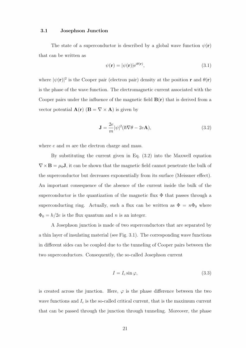
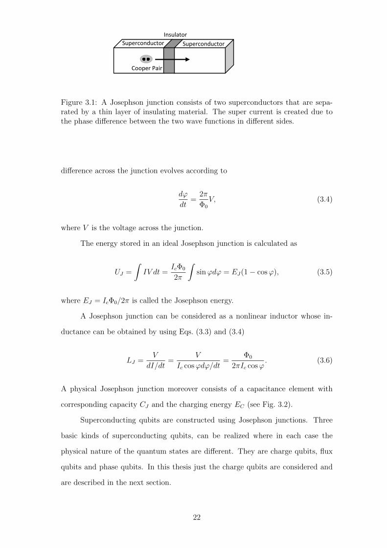
A Josephson junction is made of two superconductors that are separated by

a thin layer of insulating material (see Fig. 3.1). The corresponding wave functions

in different sides can be coupled due to the tunneling of Cooper pairs between the

two superconductors. Consequently, the so-called Josephson current

I = Ic sinϕ, (3.3)

is created across the junction. Here, ϕ is the phase difference between the two

wave functions and Ic is the so-called critical current, that is the maximum current

that can be passed through the junction through tunneling. Moreover, the phase

21

Insulator

Superconductor Superconductor

Cooper Pair

Figure 3.1: A Josephson junction consists of two superconductors that are sepa-rated by a thin layer of insulating material. The super current is created due tothe phase difference between the two wave functions in different sides.

difference across the junction evolves according to

dϕ

dt=

2π

Φ0

V, (3.4)

where V is the voltage across the junction.

The energy stored in an ideal Josephson junction is calculated as

UJ =

∫IV dt =

IcΦ0

2π

∫sinϕdϕ = EJ(1− cosϕ), (3.5)

where EJ = IcΦ0/2π is called the Josephson energy.

A Josephson junction can be considered as a nonlinear inductor whose in-

ductance can be obtained by using Eqs. (3.3) and (3.4)

LJ =V

dI/dt=

V

Ic cosϕdϕ/dt=

Φ0

2πIc cosϕ. (3.6)

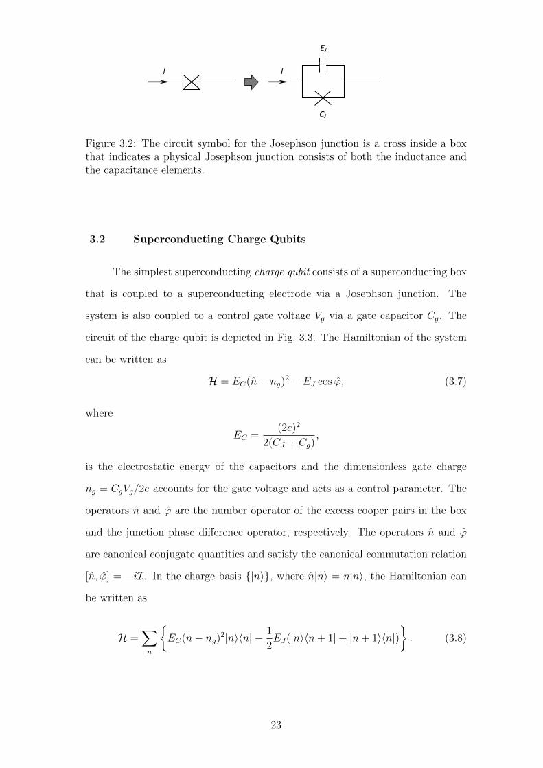
A physical Josephson junction moreover consists of a capacitance element with

corresponding capacity CJ and the charging energy EC (see Fig. 3.2).

Superconducting qubits are constructed using Josephson junctions. Three

basic kinds of superconducting qubits, can be realized where in each case the

physical nature of the quantum states are different. They are charge qubits, flux

qubits and phase qubits. In this thesis just the charge qubits are considered and

are described in the next section.

22

l

CJ

EJ

l

Figure 3.2: The circuit symbol for the Josephson junction is a cross inside a boxthat indicates a physical Josephson junction consists of both the inductance andthe capacitance elements.

3.2 Superconducting Charge Qubits

The simplest superconducting charge qubit consists of a superconducting box

that is coupled to a superconducting electrode via a Josephson junction. The

system is also coupled to a control gate voltage Vg via a gate capacitor Cg. The

circuit of the charge qubit is depicted in Fig. 3.3. The Hamiltonian of the system

can be written as

H = EC(n− ng)2 − EJ cos ϕ, (3.7)

where

EC =(2e)2

2(CJ + Cg),

is the electrostatic energy of the capacitors and the dimensionless gate charge

ng = CgVg/2e accounts for the gate voltage and acts as a control parameter. The

operators n and ϕ are the number operator of the excess cooper pairs in the box

and the junction phase difference operator, respectively. The operators n and ϕ

are canonical conjugate quantities and satisfy the canonical commutation relation

[n, ϕ] = −iI. In the charge basis |n〉, where n|n〉 = n|n〉, the Hamiltonian can

be written as

H =∑n

EC(n− ng)2|n〉〈n| − 1

2EJ(|n〉〈n+ 1|+ |n+ 1〉〈n|)

. (3.8)

23

Island

Superconductor Superconductor

Vg

Junction

Cg

Figure 3.3: A schematic representation of the charge qubit.

Here, it is assumed that the charging energy is much larger than the Josephson

energy, EC EJ , the so-called charging regime. Therefore, the first term in the

Hamiltonian (3.8) is dominant except when ng is close to a half integer number.

Considering the case ng ' 1/2, the energy splitting between the first two levels

is of order of EJ . The higher energy states however are well separated from the

two lowest energy states hence can be ignored while concentrating around the

degeneracy point ng = 1/2. Figure 3.4 shows the energy of the first two levels in

terms of the gate charge ng. The Hamiltonian (3.8) can then be written as

H = EC(ng)2|0〉〈0|+ EC(1− ng)2|1〉〈1| − 1

2EJ(|0〉〈1|+ |1〉〈0|), (3.9)

where in the language of spin-1/2 systems in terms of the Pauli matrices it takes

the form

H = −1

2Bzσz −

1

2Bxσx, (3.10)

where Bz = EC(1 − 2ng) and Bx = EJ are the bias energy and the tunneling

amplitude, respectively. The Pauli Z and X matrices are given by

σz =

1 0

0 −1

, σx =

0 1

1 0

.

24

case quasiparticle tunneling is suppressed at low tem-peratures, and a situation can be reached in which noquasiparticle excitation is found on the island.3 Underthese conditions only Cooper pairs tunnel—coherently—in the superconducting junction, and thesystem is described by the Hamiltonian

H54EC~n2ng!22EJ cos Q . (2.1)

Here n is the number operator of (excess) Cooper-paircharges on the island, and Q, the phase of the supercon-ducting order parameter of the island, is its quantum-mechanical conjugate, n52i\ ]/](\Q). The dimen-sionless gate charge, ng[CgVg/2e , accounts for theeffect of the gate voltage and acts as a control param-eter. Here we consider systems in which the chargingenergy is much larger than the Josephson coupling en-ergy, EC@EJ . In this regime a convenient basis isformed by the charge states, parametrized by the num-ber of Cooper pairs n on the island. In this basis theHamiltonian (2.1) reads

H5(n

H 4EC~n2ng!2un&^nu

212

EJ~ un&^n11u1un11&^nu!J . (2.2)

For most values of ng the energy levels are dominatedby the charging part of the Hamiltonian. However, whenng is approximately half-integer and the charging ener-gies of two adjacent states are close to each other (e.g.,at Vg5Vdeg[e/Cg), the Josephson tunneling mixes themstrongly (see Fig. 2). We concentrate on such a voltagerange near a degeneracy point where only two chargestates, say n50 and n51, play a role, while all othercharge states, having a much higher energy, can be ig-nored. In this case the superconducting charge box (2.1)reduces to a two-state quantum system (qubit) with aHamiltonian that can be written in spin-1

2 notation as

Hctrl5212

Bzsz212

Bxsx . (2.3)

The charge states n50 and n51 correspond to the spinbasis states u↑&[(0

1) and u↓&[(10), respectively. The

charging energy splitting, which is controlled by the gatevoltage, corresponds in spin notation to the z compo-nent of the magnetic field,

Bz[dEch[4EC~122ng!, (2.4)

while the Josephson energy provides the x componentof the effective magnetic field,

Bx[EJ . (2.5)

For later convenience we rewrite the Hamiltonian as

Hctrl5212

DE~h!~cos h sz1sin h sx!, (2.6)

where the mixing angle h[tan21(Bx /Bz) determines thedirection of the effective magnetic field in the x-z plane,and the energy splitting between the eigenstates isDE(h)5ABx

21Bz25EJ /sin h. At the degeneracy point,

h5p/2, it reduces to EJ . The eigenstates are denoted inthe following as u0& and u1&. They depend on the gatecharge ng as

u0&5cosh

2u↑&1sin

h

2u↓&,

u1&52sinh

2u↑&1cos

h

2u↓&. (2.7)

We can further express the Hamiltonian in the basisof eigenstates. To avoid confusion we introduce a sec-ond set of Pauli matrices r that operate in the basis u0&and u1&, while reserving the operators s for the basis ofcharge states u↑& and u↓&. By definition the Hamiltonianthen becomes

H5212

DE~h!rz . (2.8)

The Hamiltonian (2.3) is similar to the ideal single-qubit model (A1) presented in Appendix A. Ideally thebias energy (the effective magnetic field in the z direc-tion) and the tunneling amplitude (the field in the x di-rection) are controllable. However, at this stage we cancontrol—by the gate voltage—only the bias energy,while the tunneling amplitude has a constant value setby the Josephson energy. Nevertheless, by switching thegate voltage we can perform the required one-bit opera-tions (Shnirman et al., 1997). If, for example, onechooses the idle state far to the left from the degeneracypoint, the eigenstates u0& and u1& are close to u↑& and

3In the ground state the superconducting state is totallypaired, which requires an even number of electrons on theisland. A state with an odd number of electrons necessarilycosts an extra quasiparticle energy D and is exponentially sup-pressed at low T . This ‘‘parity effect’’ has been established inexperiments below a crossover temperature T*'D/(kB ln Neff), where Neff is the number of electrons in thesystem near the Fermi energy (Tuominen et al., 1992; Lafargeet al., 1993; Schon and Zaikin, 1994; Tinkham, 1996). For asmall island, T* is typically one order of magnitude lower thanthe superconducting transition temperature.

FIG. 2. The charging energy of a superconducting electron boxis shown as a function of the gate charge ng for different num-bers of extra Cooper pairs n on the island (dashed parabolas).Near degeneracy points the weaker Josephson coupling mixesthe charge states and modifies the energy of the eigenstates(solid lines). In the vicinity of these points the system effec-tively reduces to a two-state quantum system.

360 Makhlin, Schon, and Shnirman: Quantum-state engineering

Rev. Mod. Phys., Vol. 73, No. 2, April 2001

Figure 3.4: The charging energy of the first two levels of a superconducting box asa function of the gate charge ng for different numbers of the extra Cooper pairs nin the box [source: Makhlin et al. (2001)].

The Hamiltonian (3.10) corresponds to a two-state quantum system (qubit)

whose basis states are the charge states n = 0 and n = 1 that can be represented

as

|0〉 =

1

0

, |1〉 =

0

1

.

The eigenstates of the Hamiltonian (3.10) are denoted by | ↑〉 and | ↓〉 and calcu-

lated as | ↑〉 = cos η2|0〉+ sin η

2|1〉

| ↓〉 = − sin η2|0〉+ cos η

2|1〉

, (3.11)

where η = tan−1(Bx/Bz). The energy splitting between the eigenstates is given by

~Ω =√B2x +B2

z = EJ/ sin η, (3.12)

where at the degeneracy point, ng = 1/2 (η = π/2) reduces to EJ . In the new

basis | ↑〉, | ↓〉 the Hamiltonian (3.10) can be written as

H = −1

2~Ωσz, (3.13)

where σz is the Pauli Z matrix in the new basis.

The bias energy Bz in the system (3.10) can be controlled by playing with

the gate voltage ng. However, the tunneling energy Bx has a constant value that

25

depends on the Josephson energy EJ . It is possible to perform the required single-

qubit operations just by changing the gate voltage.

However, it is desirable to have control over the tunneling amplitude as

well. Actually, it is possible to obtain an effective Josephson junction with tunable

energy. To do so, the single Josephson junction is replaced by a superconducting

loop which is interrupted by two junctions, the so-called superconducting quantum

interference device (SQUID). The circuit of such charge qubit is depicted in Fig. 3.5.

The loop is also biased by an external flux Φext. If the self-inductance of the loop is

Junction

Sup

erco

nd

uct

or

Isla

nd

Sup

erco

nd

uct

or

Junction

Cg

Vg Φext

Figure 3.5: A schematic representation of a charge qubit with a SQUID insteadof a single junction. In this form of charge qubit the effective Josephson energy istunable.

low and the two junctions are identical, with the same energy E0J , the Hamiltonian

of the system takes the same form as of Eq. (3.10) but with the effective Josephson

energy for the tunneling amplitude

Bx = EeffJ (Φext) = 2E0

J cos(πΦext

Φ0

),

which is tunable. The effecting junction capacitance here is the sum of individual

capacitance of the two junctions which is CJ = 2C0J in the symmetric case.

However, experimentally it cannot be guaranteed with high precision that the

two junctions are identical. Therefore the loop is provided with three junctions

26

that gives the possibility to exactly tune the parameters.

The superconducting charge qubits are very sensitive to the charge noises.

It is possible to decrease this sensitivity by slightly changing the corresponding

circuit. In the next section the transmon qubit which is more robust against

charge noise is introduced.

3.2.1 Transmon Qubit

The charge qubits that are working in the charging regime EJ/EC 1 are

sensitive to the charge noise. This is because of the sharp dependency of the charge

qubits energy levels to the gate voltage around the degeneracy point ng = 1/2 (see

Fig. 3.4). Deviating from the degeneracy point leads to a rapid change in the

transition energy between the two levels hence results in a fast dephasing due to

the random fluctuations in the gate voltage (confer Eq. 3.11 and 3.12).

The main idea of the transmon qubit is to eliminate this problem by making

small the charge dependencies of the energy levels. This can be done by increasing

the EJ/EC ratio as it is shown in Fig. 3.6. The graphs demonstrate the charge

qubit three lowest energy levels in terms of the gate voltage ng for different values

of EJ/EC . The energy levels correspond to the energy spectrum of the Hamilto-

nian (3.7) with n = −id/dϕ. They show that the energy levels become gradually

flat as the ratio EJ/EC increased. A detailed analysis shows that the suppression

of the charge sensitivity is exponential in parameter√

8EJ/EC .

The only drawback of increasing the ratio EJ/EC is that it makes the level

spectrum to approach that of a harmonic oscillator where the levels are separated

by the same energy. However, it can be shown that while the suppression of the

charge sensitivity decreases exponentially, the anharmonicity of the levels decreases

polynomially with a small power law in EJ/EC . Therefore, it is possible to greatly

reduce the charge sensitivity of the energy levels and simultaneously have suffi-

ciently anharmonicity for the qubit operations.

27

ber of Cooper pairs transferred between the islands and thegauge-invariant phase difference between the superconduct-ors, respectively. By means of the additional capacitance CB,the charging energy EC=e2 /2C C=CJ+CB+Cg can bemade small compared to the Josephson energy. In contrast tothe CPB, the transmon is operated in the regime EJEC.

The qubit Hamiltonian, Eq. 2.1, can be solved exactly inthe phase basis in terms of Mathieu functions, see, e.g., Refs.6,16. The eigenenergies are given by

Emng = EC a2ng+km,ng− EJ/2EC , 2.2

where aq denotes Mathieu’s characteristic value, andkm ,ng is a function appropriately sorting the eigenvalues;see Appendix B for details. Plots for the lowest three energylevels E0, E1, and E2, as a function of the effective offsetcharge ng, are shown in Fig. 2 for several values of EJ /EC.One clearly observes i that the level anharmonicity dependson EJ /EC, and ii that the total charge dispersion decreasesvery rapidly with EJ /EC. Both factors i and ii influencethe operation of the system as a qubit. The charge dispersionimmediately translates into the sensitivity of the system withrespect to charge noise. A sufficiently large anharmonicity isrequired for selective control of the transitions, and the ef-fective separation of the Hilbert space into the relevant qubitpart and the rest, H=Hq Hrest. In the following sections,we systematically investigate these two factors and show thatthere exists an optimal range of the ratio EJ /EC with suffi-cient anharmonicity and charge noise sensitivity drasticallyreduced when compared to the conventional CPB.

B. The charge dispersion of the transmon

The sensitivity of a qubit to noise can often be optimizedby operating the system at specific points in parameter space.

An example for this type of setup is the “sweet spot” ex-ploited in CPBs 21. In this case, the sensitivity to chargenoise is reduced by biasing the system to the charge-degeneracy point ng=1/2, see Fig. 2a. Since the chargedispersion has no slope there, linear noise contributions can-not change the qubit transition frequency. With this proce-dure, the unfavorable sensitivity of CPBs to charge noise canbe improved significantly, potentially raising T2 times fromthe nanosecond to the microsecond range. Unfortunately, thelong-time stability of CPBs at the sweet spot still suffersfrom large fluctuations which drive the system out of thesweet spot and necessitate a resetting of the gate voltage.

Here, we show that an increase of the ratio EJ /EC leads toan exponential decrease of the charge dispersion and thus aqubit transition frequency that is extremely stable with re-spect to charge noise; see Fig. 2d. In fact, with sufficientlylarge EJ /EC, it is possible to perform experiments withoutany feedback mechanism locking the system to the chargedegeneracy point. In two recent experiments using transmonqubits, very good charge stability has been observed in theabsence of gate tuning 22,23.

Away from the degeneracy point, charge noise yieldsfirst-order corrections to the energy levels of the transmonand the sensitivity of the device to fluctuations of ng is di-rectly related to the differential charge dispersion Eij /ng,as we will show in detail below. Here Eij Ej −Ei denotesthe energy separation between the levels i and j. As expectedfrom a tight-binding treatment, the dispersion relation Emngis well approximated by a cosine in the limit of large EJ /EC,

Emng Emng = 1/4 −m

2cos2ng , 2.3

where

m Emng = 1/2 − Emng = 0 2.4

gives the peak-to-peak value for the charge dispersion of themth energy level. To extract m, we start from the exact ex-pression 2.2 for the eigenenergies and study the limit oflarge Josephson energies. The asymptotics of the Mathieucharacteristic values can be obtained by semiclassicalWKB methods see, e.g., Refs. 24–26. The resultingcharge dispersion is given by

m − 1mEC24m+5

m! 2

EJ

2ECm

2+ 3

4e−8EJ/EC, 2.5

valid for EJ /EC1. The crucial point of this result is theexponential decrease of the charge dispersion with EJ /EC.

The physics behind this feature can be understood bymapping the transmon system to a charged quantum rotor,see Fig. 3. We consider a mass m attached to a stiff, masslessrod of length l, fixed to the coordinate origin by a frictionlesspivot bearing. Using cylindrical coordinates r , ,z, the mo-tion of the mass is restricted to a circle in the z=0 plane withthe polar angle completely specifying its position. Therotor is subject to a strong homogeneous gravitational fieldg=gex in x direction, giving rise to a potential energyV=−mgl cos . The kinetic energy of the rotor can be ex-pressed in terms of its angular momentum along the z axis,

FIG. 2. Color online Eigenenergies Em first three levels, m=0,1 ,2 of the qubit Hamiltonian 2.1 as a function of the effec-tive offset charge ng for different ratios EJ /EC. Energies are givenin units of the transition energy E01, evaluated at the degeneracypoint ng=1/2. The zero point of energy is chosen as the bottom ofthe m=0 level. The vertical dashed lines in a mark the chargesweet spots at half-integer ng.

CHARGE-INSENSITIVE QUBIT DESIGN DERIVED FROM… PHYSICAL REVIEW A 76, 042319 2007

042319-3

Figure 3.6: Eigenenergies Em of first three levels (m = 0, 1, 2) of the Hamilto-

nian (3.7) in terms of the charge ng for different ratios of EJ/EC in (a) to (d).

Energies are given in units of the transition energy E01 that is evaluated at the

point ng = 1/2. The dashed lines in (a) correspond to the half-integer values of ng

[source: Koch et al. (2007)].

V

CB

Cg

Φext

Figure 3.7: Effective circuit diagram of the transmon qubit. The circuit consists of

a SQUID that is biased with the flux Φext and equipped with an additional large

capacitance element CB.

The circuit of the transmon qubit is shown in Fig. 3.7. The Hamiltonian of

28

the circuit is given by Eq. (3.7) where the charging energy

EC =(2e)2

2(CJ + CB + Cg)

can be made small compared to the junction energy by means of the additional

capacitance CB.

In order to control the state of the transmon qubit and performing logic gates,

the qubit is embedded in a superconducting transmission line resonator. Such a

setup which is called circuit quantum electrodynamics (circuit QED) provides also

a system for coupling several transmon qubits to perform multiqubit quantum

gates. The next section is devoted to explain the cirquit QED setup.

3.3 Circuit Quantum Electrodynamics

To implement two-qubit gates the pairs of qubit should be coupled together

and the interaction between them be controlled. There are various methods to cou-

ple the superconducting qubits together. One possibility is to connect the super-

conducting boxes directly via a capacitor which results in an Ising type interaction

term, σkzσlz in the Hamiltonian. Another way is to connect the superconducting

circuits in parallel to a common LC oscillator which results in an interaction term

of type σkyσly where the Pauli σy is given by

σy =

0 −i

i 0

.

The method which is discussed here is to couple the superconducting qubits

to a single mode of a transmission line resonator. A transmission line resonator is a

device where an electromagnetic field is guided along it from one point to another.

The length of the transmission line can be much longer than the wavelength of the

field that is contained by it. It is possible to model the transmission line resonator

by a circuit of infinitely many of infinitesimal LC oscillators. The Hamiltonian of

29

the transmission line resonator is then proved to be

H =∞∑n=1

~ωn(a†nan + 1/2). (3.14)

Eq. (3.14) is the Hamiltonian of an infinite set of independent harmonic oscillators

where a† and a are creation and annihilation operators, respectively, and ωn are

the frequencies corresponding to the resonator modes. In many situations it is

sufficient to keep just a single resonator mode hence the Hamiltonian takes the

form

H = ~ωr(a†a+ 1/2), (3.15)

where ωr is some specified mode frequency.

Figure 3.8 shows the circuit QED architecture. The transmission line res-

onator consists of a full-wave section of superconducting coplanar waveguides. The

superconducting charge qubit is placed between the two superconducting lines and

capacitively coupled to the central line where the voltage standing wave is in max-

imum. In this case the Hamiltonian of the qubit is similar to Eq. 3.8 however the

dimensionless gate charge ng should be replaced by

ng =Cg2e

(V dcg + v) = ndcg +

Cg2ev,

where V dcg is the dc part of the voltage and v is the quantum part of the voltage

due to the resonator. The latter is given by

v =

√~ωrcL

(a† + a),

where L is the resonator length and c denotes the capacitance per unit length of

the transmission line.

30

For large detuning,g/D!1, expansion of Eq.(4) yieldsthe dispersive spectrum shown in Fig. 1(c). In this situation,the eigenstates of the one excitation manifold take the form[15]

u− ,0l , − sg/Ddu↓,0l + u↑,1l, s7d

u+ ,0l , u↓,0l + sg/Ddu↑,1l. s8d

The corresponding decay rates are then simply given by

G− ,0 . sg/Dd2g + k, s9d

G+ ,0 . g + sg/Dd2k. s10d

More insight into the dispersive regime is gained by mak-ing the unitary transformation

U = expF g

Dsas+ − a†s−dG s11d

and expanding to second order ing (neglecting damping forthe moment) to obtain

UHU† < "Fvr +g2

DszGa†a +

"

2FV +

g2

DGsz. s12d

As is clear from this expression, the atom transition is acStark/Lamb shifted bysg2/Ddsn+1/2d. Alternatively, onecan interpret the ac Stark shift as a dispersive shift of thecavity transition byszg2/D. In other words, the atom pullsthe cavity frequency by ±g2/kD.

III. CIRCUIT IMPLEMENTATION OF CAVITY QED

We now consider the proposed realization of cavity QEDusing the superconducing circuits shown in Fig. 2. A 1Dtransmission line resonator consisting of a full-wave sectionof superconducting coplanar waveguide plays the role of thecavity and a superconducting qubit plays the role of theatom. A number of superconducting quantum circuits couldfunction as artificial atom, but for definiteness we focus hereon the Cooper-pair box[6,16–18].

A. Cavity: Coplanar stripline resonator

An important advantage of this approach is that the zero-point energy is distributed over a very small effective volume(<10−5 cubic wavelengths) for our choice of a quasi-one-dimensional transmission line “cavity.” As shown in Appen-dix A, this leads to significant rms voltagesVrms

0 ,Î"vr /cLbetween the center conductor and the adjacent ground planeat the antinodal positions, whereL is the resonator length andc is the capacitance per unit length of the transmission line.At a resonant frequency of 10 GHzshn /kB,0.5 Kd and fora 10mm gap between the center conductor and the adjacentground plane,Vrms,2 mV corresponding to electric fieldsErms,0.2 V/m, some 100 times larger than achieved in the3D cavity described in Ref.[3]. Thus, this geometry mightalso be useful for coupling to Rydberg atoms[19].

In addition to the small effective volume and the fact thatthe on-chip realization of CQED shown in Fig. 2 can befabricated with existing lithographic techniques, atransmission-line resonator geometry offers other practicaladvantages over lumpedLC circuits or current-biased largeJosephson junctions. The qubit can be placed within the cav-ity formed by the transmission line to strongly suppress thespontaneous emission, in contrast to a lumpedLC circuit,where without additional special filtering, radiation and para-sitic resonances may be induced in the wiring[20]. Since theresonant frequency of the transmission line is determinedprimarily by a fixed geometry, its reproducibility and immu-nity to 1/f noise should be superior to Josephson junctionplasma oscillators. Finally, transmission-line resonances incoplanar waveguides withQ,106 have already been dem-onstrated[21,22], suggesting that the internal losses can bevery low. The optimal choice of the resonatorQ in this ap-proach is strongly dependent on the intrinsic decay rates ofsuperconducting qubits which, as described below, are pres-ently unknown, but can be determined with the setup pro-posed here. Here we assume the conservative case of anovercoupled resonator with aQ,104, which is preferable forthe first experiments.

B. Artificial atom: The Cooper-pair box

Our choice of “atom,” the Cooper-pair box[6,16], is amesoscopic superconducting island. As shown in Fig. 3, the

FIG. 2. (Color online). Schematic layout and equivalent lumpedcircuit representation of proposed implementation of cavity QEDusing superconducting circuits. The 1D transmission line resonatorconsists of a full-wave section of superconducting coplanar wave-guide, which may be lithographically fabricated using conventionaloptical lithography. A Cooper-pair box qubit is placed between thesuperconducting lines and is capacitively coupled to the center traceat a maximum of the voltage standing wave, yielding a strong elec-tric dipole interaction between the qubit and a single photon in thecavity. The box consists of two smalls,100 nm3100 nmd Joseph-son junctions, configured in a,1 mm loop to permit tuning of theeffective Josephson energy by an external fluxFext. Input and out-put signals are coupled to the resonator, via the capacitive gaps inthe center line, from 50V transmission lines which allow measure-ments of the amplitude and phase of the cavity transmission, andthe introduction of dc and rf pulses to manipulate the qubit states.Multiple qubits (not shown) can be similarly placed at differentantinodes of the standing wave to generate entanglement and two-bit quantum gates across distances of several millimeters.

CAVITY QUANTUM ELECTRODYNAMICS FOR… PHYSICAL REVIEW A 69, 062320(2004)

062320-3

Figure 3.8: Schematic representation of the circuit QED and its equivalent lumpedcircuit. The transmission line resonator consists of a full-wave section of super-conducting coplanar waveguide. The transmon qubit is placed between the su-perconducting lines and capacitively coupled to the central line where the voltagestanding wave is in maximum [source: Blais et al. (2004)].

The total Hamiltonian of the system can then be written as

H =∑n

EC(n− ndcg +

Cg2ev)2|n〉〈n| − 1

2EJ(|n〉〈n+ 1|+ |n+ 1〉〈n|)

+ ~ωra†a, (3.16)

where the second term is the Hamiltonian of the oscillator while neglecting the

zero-point energy.

Focusing on ndcg ' 1/2 it is possible to keep just the two lowest states, n = 0, 1

(see section 3.2). The Hamiltonian (3.16) can be written as

H = −1

2EC(1− 2ndcg )σz −

1

2EJσx

− eCg(Cg + CJ)

√~ωrcL

(a† + a)(1− 2ndcg − σz) + ~ωra†a, (3.17)

where the Pauli matrices are described in terms of the basis |0〉, |1〉. After

rotating the basis to | ↑〉, | ↓〉 the Hamiltonian (3.17) takes the form

H = −1

2~Ωσz − ~g(a† + a)(1− 2ndcg − cos ησz + sin ησx) + ~ωra†a, (3.18)

31

where

Ω =1

~

√E2J + E2

C(1− 2ndcg )2,

η = tan−1(EJ/EC(1− 2ndcg ),

g =eCg

~(Cg + CJ)

√~ωrcL

,

and σz and σx are the Pauli matrices after expressing in terms of the new basis. At

the degeneracy point where ndcg = 1/2 (η = π/2) applying the so-called rotating

wave approximation reduces the Hamiltonian (3.18) to

H = −1

2~Ωσz − ~g(a†σ− + aσ+) + ~ωra†a (3.19)

where σ± = (σx ± iσy)/2 and all the overlines have been dismissed for simplicity.

The Hamiltonian (3.19) is the so-called Jayness-Cummings Hamiltonian.

Up to this point it has been described how to couple a qubit to a transmission

line resonator. In the rest of this section it is described how to realize single- and

multi- qubit operations.

Single qubit gates can be realized by microwaves drive pulses applied on the

resonator. A microwave drive can be described by the Hamiltonian

Hd = εd(t)(a†e−iωdt + aeiωdt) (3.20)

where εd(t) is the amplitude and ωd the frequency of the drive. To see the effect

of the drive on the qubit the microwave drive Hamiltonian (3.20) is added to the

Hamiltonian (3.19) and the total Hamiltonian is undergone the transformation

U(H +Hd)U† with U is given by

U = exp[ g

∆(aσ+ − a†σ−)

], (3.21)

where ∆ = Ω − ωr is called detuning. For large values of detuning compared to

32

the coupling g (small values of g/∆) expanding the transformation to the second

order in g/∆ results

U(H +Hd)U† ≈ ~

2[Ω− ωd + 2

g2

∆(a†a+

1

2)]σz + ~

g

∆εd(t)σx+

~(ωr − ωd)a†a+ ~εd(t)(a† + a), (3.22)

in a frame rotating at the drive frequency ωd. Depending on the frequency and

amplitude of the drive different quantum gates can be realized.

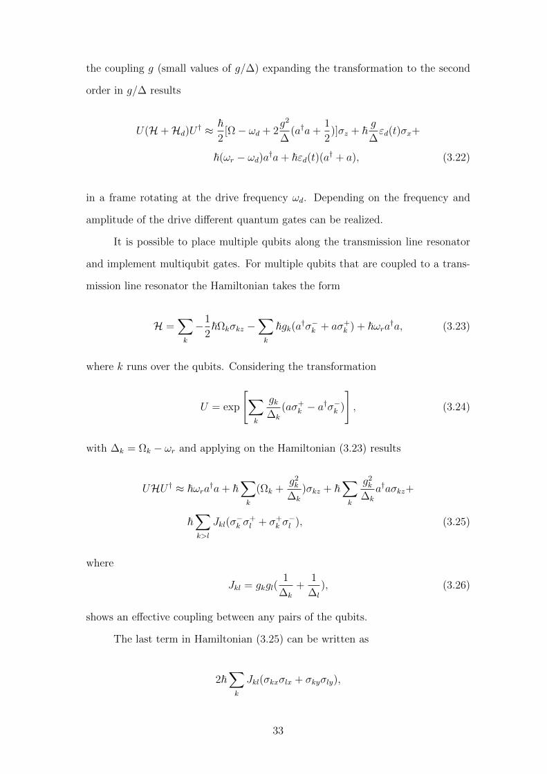
It is possible to place multiple qubits along the transmission line resonator

and implement multiqubit gates. For multiple qubits that are coupled to a trans-

mission line resonator the Hamiltonian takes the form

H =∑k

−1

2~Ωkσkz −

∑k

~gk(a†σ−k + aσ+k ) + ~ωra†a, (3.23)

where k runs over the qubits. Considering the transformation

U = exp

[∑k

gk∆k

(aσ+k − a†σ−k )

], (3.24)

with ∆k = Ωk − ωr and applying on the Hamiltonian (3.23) results

UHU † ≈ ~ωra†a+ ~∑k

(Ωk +g2k

∆k

)σkz + ~∑k

g2k

∆k

a†aσkz+

~∑k>l

Jkl(σ−k σ

+l + σ+

k σ−l ), (3.25)

where

Jkl = gkgl(1

∆k

+1

∆l

), (3.26)

shows an effective coupling between any pairs of the qubits.

The last term in Hamiltonian (3.25) can be written as

2~∑k

Jkl(σkxσlx + σkyσly),

33

which shows an XY type interaction between any pair of the qubits. Evolution of

the system under such coupling together with the single qubit manipulation can

be used to realize CNOT gate.

However, as it was mentioned in section 2.1.2 it is possible to design mi-

crowave drive pulses to realize the multiqubit gates directly. In the next chapter

it is described how to design a set of microwave pulses to realize the three qubit

Toffoli gate.

34

Chapter 4

Implementation of the Toffoli Gate in

Systems with Imperfections

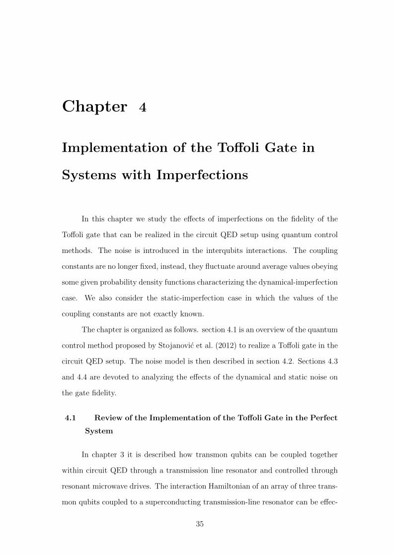
In this chapter we study the effects of imperfections on the fidelity of the

Toffoli gate that can be realized in the circuit QED setup using quantum control

methods. The noise is introduced in the interqubits interactions. The coupling

constants are no longer fixed, instead, they fluctuate around average values obeying

some given probability density functions characterizing the dynamical-imperfection

case. We also consider the static-imperfection case in which the values of the

coupling constants are not exactly known.

The chapter is organized as follows. section 4.1 is an overview of the quantum

control method proposed by Stojanovic et al. (2012) to realize a Toffoli gate in the

circuit QED setup. The noise model is then described in section 4.2. Sections 4.3

and 4.4 are devoted to analyzing the effects of the dynamical and static noise on

the gate fidelity.

4.1 Review of the Implementation of the Toffoli Gate in the Perfect

System

In chapter 3 it is described how transmon qubits can be coupled together

within circuit QED through a transmission line resonator and controlled through

resonant microwave drives. The interaction Hamiltonian of an array of three trans-

mon qubits coupled to a superconducting transmission-line resonator can be effec-

35

tively described by an XY -type (flip-flop) Hamiltonian

H0 =∑i<j

Jij (σixσjx + σiyσjy) , i, j = 1, 2, 3 (4.1)

where Jij are coupling constants and σix and σiy are Pauli X and Y matrices,

respectively. This system is manipulated by a Zeeman-like Hamiltonian

Hc(t) =3∑i=1

[u(i)x (t)σix + u(i)

y (t)σiy], (4.2)

with control fields u(i)x (t) and u

(i)y (t) affecting the qubits in x and y directions.

Therefore, the system dynamics is governed by the total Hamiltonian

H(t) = H0 +Hc(t). (4.3)

These control fields can be implemented through wave generators. However,

to keep the transmon qubits well-defined two-level systems, the fields cannot be

arbitrarily large. The norm

umax = maxi,t

√[u

(i)x (t)]2 + [u

(i)y (t)]2 (4.4)

is then restricted to be smaller than some threshold value.

The controllability of the system can be verified by considering the Lie al-

gebra generated by span−iH0,−iσjx,−iσjy; j = 1, 2, 3 which is actually the Lie

algebra su(8). This algebra provides the operator controllability of the system.

Finding the control fields that implement the Toffoli gate is a numerical

optimization problem. A given gate time tg is divided into Nt (even number)

intervals of the same time length T . Then, the set of fields is supposed to be

constant in each interval and is acting on the related qubits alternating between

the x and y directions.

In the first interval 0 ≤ t ≤ T , three x-control pulses with constant ampli-

36

tudes u(i)x,1 are applied to all three qubits. The dynamics is then governed by the

Hamiltonian

Hx,1 = H0 +3∑i=1

u(i)x,1σix. (4.5)

In the second interval T ≤ t ≤ 2T , the y-control pulses with amplitudes u(i)y,1 are

applied leading to the Hamiltonian

Hy,1 = H0 +3∑i=1

u(i)y,1σiy. (4.6)

This process is repeated Nt/2 times to complete all Nt intervals. These time-

independent Hamiltonians for each interval lead to the time evolution operators

Ux,n = exp(−iHx,nT ) (4.7)

Uy,n = exp(−iHy,nT ) (4.8)

respectively in corresponding intervals, where n = 1, . . . , Nt/2. The product

Uy,nUx,n in the reverse order, is the time evolution operator U(t = tg).

The values of the 3Nt control fields are obtained through maximizing the

fidelity

F =1

8

∣∣ Tr[U † (tg, Nt,u, Jij)UToff

] ∣∣ , (4.9)

where u is the concatenation of all control pulses and UToff is the Toffoli gate that

is given in Eq. (2.7). The optimized control fields are obtained through numerical

maximization of the fidelity with an initial guess for the fields. The minimum gate

time for a given fidelity can also be obtained by starting with a sufficiently large tg

and then gradually decreasing its value. The values of Nt and T that are related

through tg = NtT should be selected such that the corresponding pulse sequence

can be generated experimentally.

The piecewise-constant control pulses obtained here can be filtered through

a low-pass filter such that they can be generated by an actual wave generator.

Using the product formula approach suggested in Heule et al. (2010), it is possible

37

to obtain the fidelities for the filtered control fields.

Assuming umax < 130 MHz, J = 30 MHz and J12 = J23 = 6J13 = J , the

Toffoli gate can be realized with a fidelity larger than 99% in 4.18J−1 = 140 ns

with Nt = 20 control intervals. In the following sections we focus on this specific

realization.

4.2 Noise Model

In this section we introduce our noise model that is applied to simulate the

imperfections in the Toffoli gate implementation. We are specially interested in

the case where the interactions between the qubits are noisy. Each Jij in Eq. (4.1)

is considered to be independently coupled to a stochastic variable described by

Jij(t) = Jij (1 + εij(t)) , (4.10)

where Jij are average coupling strengths and εij(t) are independent Gaussian ran-

dom variables for different subindices. This noise model has been used in many

physical contexts and can be seen as an effective behavior when we average out

the effect of the environment over the main system (Strack and Sachdev, 2011).

We suppose that all εij(t) have the same mean and variance and change their

values in time simultaneously with a fixed frequency fc. Then, they remain fixed

during the time interval τc = 1/fc:

ε(t) = ε(k), (k − 1)τc ≤ t < kτc, (4.11)

where we have omitted the subindices because all components have the same be-

havior. The random variables ε(k) are supposed to be independent and identically

distributed (iid) Gaussian random variables in different time intervals with expec-

tation E[ε(k)] = 0 and variance E[(ε(k))2] = σ2 < ∞, where k runs over integer

values.

38

The autocorrelation function, R(τ), for ε(t) can be calculated as

R(τ) = 〈ε(t)ε(t+ τ)〉 (4.12)

= limtM→∞

1

2tM

∫ +tM

−tMε(t)ε(t+ τ)dt

= limM→∞

1

2(Mτc + ∆tM)

∫ +(Mτc+∆tM )

−(Mτc+∆tM )

ε(t)ε(t+ τ)dt,

where tM can be written as Mτc + ∆tM with some integer M and 0 ≤ ∆tM < τc.

Moreover, τc is supposed to be finite and different from zero. In order to calculate

the last integral in Eq. (4.12), first we note that

∫ kτc

(k−1)τc

ε(t)ε(t+ τ)dt =

∫ kτc−τ

(k−1)τc

ε(t)ε(t+ τ)dt︸ ︷︷ ︸I

+

∫ kτc

kτc−τε(t)ε(t+ τ)dt︸ ︷︷ ︸

II

,

where 0 ≤ τ ≤ τc and the right hand side integrals are calculated as

I =

∫ kτc−τ

(k−1)τc

ε(k)ε(k)dt = (ε(k))2

∫ kτc−τ

(k−1)τc

dt = (ε(k))2(τc − τ),

II =

∫ kτc

kτc−τε(k)ε(k+1)dt = ε(k)ε(k+1)

∫ kτc

kτc−τdt = ε(k)ε(k+1)τ.

Therefore,

R(τ) = limM→∞

1

2(Mτc + ∆tM)((τc − τ)

M∑k=−M

(ε(k))2 + τM∑

k=−M

ε(k)ε(k+1) +Res(∆tM)

),

where the residual function Res(∆tM) is bounded,

Res(∆tM) ≤ |(τc − τ)(ε(k))2|+ |τε(k)ε(k+1)| <∞.

Having performed the same calculations in the case of −τc ≤ τ ≤ 0 we finally

39

obtain

〈ε(t)ε(t+ τ)〉 =

(

1− |τ |τc

)σ2, −τc ≤ τ ≤ τc

0, otherwise.(4.13)

The power spectral density (Fourier transform of the autocorrelation func-

tion), which displays the essence of the noise, is given by

S(ω) =σ2τc√

2πsinc2

(ωτc2

). (4.14)

In section 4.3 we describe how we simulate the effect of noise on the fidelity

for values of τc such that τc ≤ tg where tg is the gate time. For τc > tg we are only

interested in the limit τc → ∞. In this case the power spectral density function

approaches to the delta function on zero, which corresponds to a fixed noise in the

system. It means that the value of the random variable remains fixed for ever.

Physically, this situation is associated with inaccuracies in the system parameters.

This situation is analyzed in section 4.4.

4.3 Analyzing the Dynamical Imperfections

Using the noise model introduced in the previous section, we analyze here

the implementation of the Toffoli gate when the system is affected by dynamical

imperfections. We actually investigate how the gate fidelity is affected by the noise

in the system. Then, the system Hamiltonian Eq. (4.1) undergoes noise while the

control Hamiltonian Eq. (4.2) is maintained perfect (without noise). The scenario

is to apply a set of control fields optimized for the perfect system to an imperfect

system. In other words, we analyze the sensitivity of the control fields to the noise

in the main system.

We start by obtaining a set of optimal control fields implementing the Toffoli

gate in the perfect system. The fields can be found by maximizing the fidelity

given by Eq. (4.9) using the parameter values given at the end of section 4.1. To

be close enough to the global optimal solution, we carry the maximization process

over 200 random initial guesses and then select the set of fields with largest fidelity.

40

In our noisy system, the couplings Jij in Eq. (4.1) remain no longer fixed

and evolve according to Eq. (4.10). There are three different coupling constants

and, in principle, the noise affect each of them independently. We are imposing

that J12 = J23 = 6J13 = J and we are assuming that the random variables εij(t)

associated with those couplings have the same mean, variance and characteristic

frequency. Under those assumptions, we will show later on in this section that

introducing the noise only in J is essentially equivalent to introduce the noise in

the three coupling constants. This explains why we can drop the subindices of

εij(t) and call the random variable simply by ε(t).

Let ε(t) change its value with a fixed frequency fc = 1/τc. We generate tgfc

random numbers independently according to a Gaussian distribution with a zero

mean and standard deviation σ. Accordingly, we have a realization of ε(t) as

ε(t) =

tgfc∑k=1

ε(k)χ[(k−1)τc,kτc) t ∈ [0, tg), (4.15)

and therefore J(t) according to Eq. (4.10). The function χ is defined as

χ[(k−1)τc,kτc) =

1, t ∈ [(k − 1)τc, kτc)

0, otherwise.(4.16)

We also set the value of fc such that the product tgfc becomes integer.

It is now possible to calculate the time evolution operator for the noisy

system using the total Hamiltonian H0(J(t))+Hc(t) with those values of J(t) above

realized. Here, we just note that for T/τc > 1 each term in Eqs. (4.7) and (4.8) is

replaced by a product of exponentials of time-independent Hamiltonians in each

τc. The corresponding fidelity for that realization can then be calculated using

Eq. (4.9).

The next step is to calculate the average fidelity, which is obtained by re-

peating the above process with the same fc and σ for a large number of realizations

of ε(t) within the corresponding time interval and summing over all fidelities and

41

dividing by the total number of realizations. Finally, using this method systemat-

ically, we obtain the fidelity as a function of σ with a fixed fc.

Figure 4.1 shows the average fidelity as a function of σ for tgfc = 200, 100, 40,

20, 10, 5, 2, 1 from top to bottom, respectively. The number of realizations per each

fixed σ for the first four items is 10,000 and for the last four items is 100,000.

The average fidelity decreases for all frequencies when the standard deviation σ

increases, confirming our intuition about the effect of the decoherence over the

coherent evolution. Notice that the average fidelity quickly drops to small values

specially when tgfc = 5.

For a given σ, the fidelity is less affected when the noise characteristic fre-

quency is high (tgfc 1). In other words, the high-frequency noise generates less

decoherence. This observation in our simulations can be justified first of all in

terms of our noise model specially by looking at the power spectral density given

by Eq. (4.14). As the noise frequency increases (τc → 0), the power spectral den-

sity function approaches zero for all ω. This means that the noise disappears and

the fidelity remains unaffected.

However, an alternative way to analyze this result is using the theorem given

by Facchi et al. (2005). The time evolution of the system over each control time

T = τcN is given by

UN(T ) =N∏k=1

exp[−i(H + ε(k)H0)τc], (4.17)

where H0 and H are obtained from H0 and H, Eq. (4.1) and Eq. (4.3) respectively,

after replacing Jij by Jij. Expanding the product, we can write the result up

to the first power of T as

1− iHT − iH0T

N

N∑k=1

ε(k).

42

But according to the weak law of large numbers

limN→∞

(∣∣∣∣∣ 1

N

N∑k=1

ε(k) − E[ε(k)]

∣∣∣∣∣ > ε

)= 0, (4.18)

and thus the first power of H0T as well as all the higher powers approach zero in

probability, hence

limN→∞

(‖ UN(T )− exp(−iHT ) ‖> ε

)= 0. (4.19)

Therefore, the effect of noise disappears if the characteristic frequency τ−1c is suf-

ficiently high.

The validity of Eq. (4.19) can be also verified by decreasing the number of

realizations, that is, performing an average with smaller samples. In this case,

the resulting plots will be no longer smooth. Actually, the points in each plot

are scattered around the average curve. However, the smoothness of the plots

corresponding to high frequencies are less affected. In another words, the plots for

higher frequencies are less sensitive to the number of realizations.

However, using the central limit theorem, η = limN→∞∑N

k=1 ε(k)/√N goes

to a Gaussian distribution with the same mean and variance of ε(k). Therefore, for

finite but large N Facchi et al. (2005)

UN(T ) ∼ exp(−iHT ) exp(−iηH0T/√N), (4.20)

which shows how the error enters in each control step T of the implementation

and the errors will eventually reduce the gate fidelity. This result is not valid for

intermediate values of N , since the terms corresponding to the nonzero commutator

brackets of H0 and H become also important.

Figure 4.1 also shows that for a fixed σ the average fidelity decreases when

we decrease the noise frequency from tgfc = 200 until tgfc = 5 and the fidelity

has the opposite behavior from tgfc = 5 until tgfc = 1. This behavior can be

43

explained from the effect of the control pulses on an imperfect system. When the

control-pulse frequency is close to the noise frequency, τ−1c = T−1, its effect helps

to protect the system against decoherence, similar to dynamical decoupling Viola

et al. (1999); Lidar (2012). When we increase the noise frequency, the control-field

effect becomes less relevant, and for tgfc > 5 it plays almost no role at all.

Finally, Figure 4.1 shows that the curves apparently converge to the same

average fidelity for sufficiently large σ. The limiting average fidelity is close to

1/d = 0.125, which corresponds to the one obtained from the full randomizing map

ε(ρ) = I/d, where ρ is an arbitrary (pure) state and d the Hilbert space dimension.

However, this saturation value (0.125) can be obtained if the randomness in the

gate parameters uniformly generates all elements in SU(8), and if we end up in a

Lie subgroup of SU(8), the saturation value can be different (Heule et al., 2010).

What we observe after performing simulations with large values of σ is that the

saturation values are not exactly the same, but slightly different depending on the

noise frequency. Therefore, fixing the control Hamiltonian and just changing the

coupling J does not seem to generate the whole SU(8) space. Figure 4.4 shows

the average fidelities for large values of standard deviation.

Now, we come back to justify why introducing one source of noise to J is

sufficient to obtain essentially the same results of having three independent sources

of noise affecting three couplings J12, J13, J23. In the latter case, the exponent

in Eq. (4.17) is replaced by

−i(H + ε(k) · H0)τc,

where

ε(k) = (ε(k)12 , ε

(k)13 , ε

(k)23 ), (4.21)

H0 = (H12, H13, H23), (4.22)

44

and

Hij = Jij (σixσjx + σiyσjy) , i < j. (4.23)

By using η = limN→∞∑N

k=1 ε(k)/√N instead of η, a similar reasoning to the

one used for one J can be applied here to reach the same results as before for

high noise frequencies. Moreover, we have repeated the simulations with three

independent sources of noise and found essentially the same results for low noise

frequencies as well. Figure 4.2 shows the average fidelity as a function of σ in the

case of three independent sources of noise. Actually, increasing the number of noise

sources just leads to faster decay of average fidelity for all frequencies. Simulations

with six different couplings (different couplings in X and Y directions) and with

six independent sources of noise confirm the latter statement. Figure 4.3 shows

the average fidelity as a function of σ in the case of six independent sources of

noise. Moreover, in the new simulations, there is no universal saturation value.

Figures 4.5 and 4.6 show the average fidelities for large values of standard deviation

in the cases of three and six sources of noise.

4.4 Analyzing the Static Imperfection

As we have discussed at the end of section 4.2, the case τc →∞ corresponds

to a fixed noise in the system, that is, the noise does not change in time. Such

a static noise can be associated with, for example, inaccessibility of measuring

exactly the system parameters such as the coupling constants. Static noises do not

lead to any decoherence, but introduce error into the gate implementation. It is

known that entanglement dynamics in similar systems remain almost unchanged

under the influence of uniform static noise when it is smaller than 10% (Tsomokos

et al. (2007, 2008)).

Analyzing the error for the static-imperfections case is mathematically equiv-

alent to the case of dynamical noise with τ−1c = t−1

g . Again, we adjust the control

Hamiltonian for the perfect system and use it for a system with static imperfec-

tions. The coupling is given by Eq. (4.10) with a fixed random variable ε(t) = ε for

45

the whole evolution. Considering a uniform distribution for ε, we generate a large

sample of couplings with a given half-width δ and then calculate the correspond-

ing fidelity using Eq. (4.9). After obtaining the sample average and repeating the

procedure for many values of δ, we find how the fidelity changes as a function of

the half-width. Moreover, we have decreased the noise level interval to be more

focused on the region with unaffected entanglement.

Figure 4.7 depicts the average fidelity as a function of the half-width δ.

The number of realizations per each fixed δ is 100,000. The diagram shows that

the average fidelity decreases when the half-width δ increases. Here, we have

focused on half-widths less than 0.5 because the experimental upper bound for

such superconducting qubit chain is quite below that (Tsomokos et al., 2007).

Actually for disorders such as δ ≤ 10%, the average fidelity remains above 97.83%.

Specifically, the fidelity decreases by 2% when the system affected by a uniform

noise with half-width less than 10%.

Actually, it is possible to obtain a more robust Toffoli gate that has a better

performance while affected by the static uniform noise. In the next chapter we

obtain a more robust gate by modifying the quantum optimization problem by

using a weighted average of the fidelity over an interval of coupling values as the

objective functional.

4.5 Summary and Conclusions

In this chapter we considered the effect of imperfections on a recently estab-

lished Toffoli gate realized in circuit QED with quantum control methods. The

implementation of the gate has been discussed in more details by Stojanovic et al.

(2012). The total Hamiltonian here is bilinear and we studied the effect of imperfec-

tions on the system Hamiltonian by introducing noise in the interqubit couplings.

We showed that in the case of dynamical imperfections the average fidelity is less

sensitive to noise for high characteristic frequencies. Actually the effect of noise

completely disappears when the noise frequency is sufficiently high. For static

46

noise we showed that the fidelity decreases by 2% when the system affected by

a uniform noise with half-width less than 10%. The results in this chapter have

been also discussed in (Moqadam et al., 2013) that is recently published in physical

review A.

Actually, the results in Stojanovic et al. (2012) as well as those were discussed

in this chapter are valid under the two-level approximation, i.e., in the absence of

any significant leakage from the two-state computational subspace of the transmon

qubits. The parameter imperfections studied here can likely be incorporated in an

analogous fashion within a more complete multi-level analysis.

47

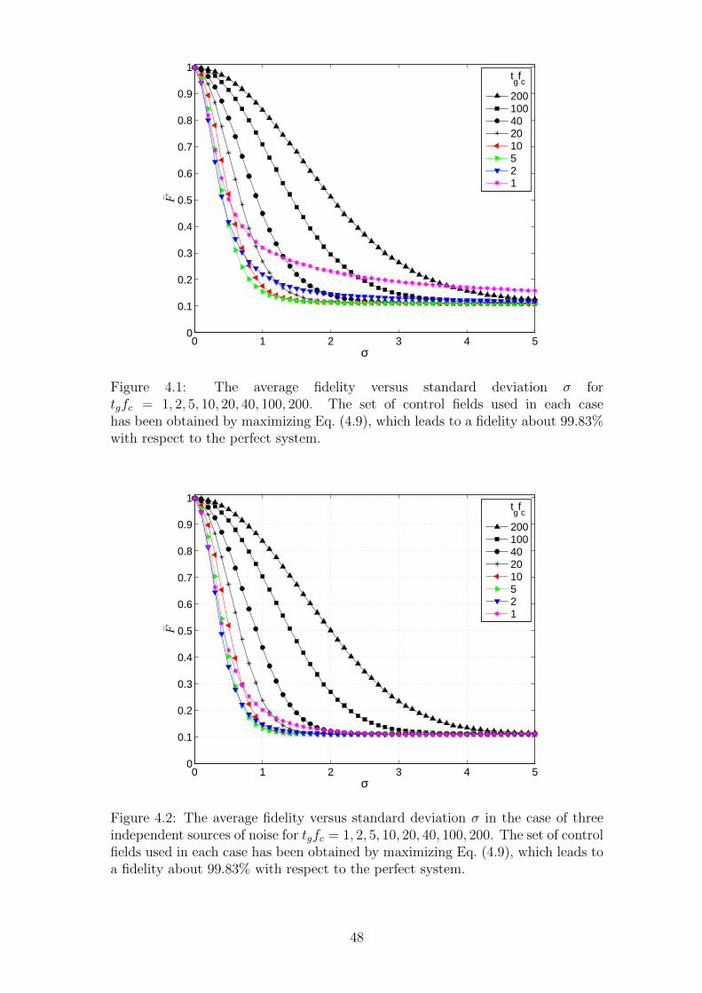
0 1 2 3 4 50

0.1

0.2

0.3

0.4

0.5

0.6

0.7

0.8

0.9

1

σ

F

tgfc

200100402010521

Figure 4.1: The average fidelity versus standard deviation σ fortgfc = 1, 2, 5, 10, 20, 40, 100, 200. The set of control fields used in each casehas been obtained by maximizing Eq. (4.9), which leads to a fidelity about 99.83%with respect to the perfect system.

0 1 2 3 4 50

0.1

0.2

0.3

0.4

0.5

0.6

0.7

0.8

0.9

1

σ

F

tgfc

200100402010521

Figure 4.2: The average fidelity versus standard deviation σ in the case of threeindependent sources of noise for tgfc = 1, 2, 5, 10, 20, 40, 100, 200. The set of controlfields used in each case has been obtained by maximizing Eq. (4.9), which leads toa fidelity about 99.83% with respect to the perfect system.

48

0 1 2 3 4 50

0.1

0.2

0.3

0.4

0.5

0.6

0.7

0.8

0.9

1

σ

F

tgfc

200100402010521

Figure 4.3: The average fidelity versus standard deviation σ in the case of sixindependent sources of noise for tgfc = 1, 2, 5, 10, 20, 40, 100, 200. The set of controlfields used in each case has been obtained by maximizing Eq. (4.9), which leads toa fidelity about 99.83% with respect to the perfect system.

1000 2000 3000 4000 5000 6000 7000 8000 9000 100000.1

0.11

0.12

0.13

0.14

0.15

0.16

0.17

0.18

0.19

0.2

σ

F

tgfc

200100402010521

Figure 4.4: The average fidelity versus standard deviation at large values of σ inthe case of single source of noise for tgfc = 1, 2, 5, 10, 20, 40, 100, 200.

49

1000 2000 3000 4000 5000 6000 7000 8000 9000 100000.1

0.11

0.12

0.13

0.14

0.15

0.16

0.17

0.18

0.19

0.2

σ

F

tgfc

200100402010521

Figure 4.5: The average fidelity versus standard deviation at large values of σ inthe case of three sources of noise for tgfc = 1, 2, 5, 10, 20, 40, 100, 200.

1000 2000 3000 4000 5000 6000 7000 8000 9000 100000.1

0.11

0.12

0.13

0.14

0.15

0.16

0.17

0.18

0.19

0.2

σ

F

tgfc

200100402010521

Figure 4.6: The average fidelity versus standard deviation at large values of σ inthe case of six sources of noise for tgfc = 1, 2, 5, 10, 20, 40, 100, 200.

50

0 0.1 0.2 0.3 0.4 0.50.5

0.55

0.6

0.65

0.7

0.75

0.8

0.85

0.9

0.95

1

δ

F

0 0.02 0.04 0.06 0.08 0.10.97

0.975

0.98

0.985

0.99

0.995

1

Figure 4.7: The average fidelity versus half-width δ in the case of static imperfec-tions. The set of control fields used here has been obtained by maximizing Eq. (4.9),which leads to a fidelity about 99.83% with respect to the perfect system. Inset:a zoom on the region 0 ≤ δ ≤ 0.1.

51

Chapter 5

Improving the Gate Fidelity in Systems

with Imperfections

In chapter 4, we considered the set of control fields optimized for a fixed value

of coupling and then applied that set to a system with imperfections. Actually, we

have investigated there the performance of that specific set of fields in the presence

of noise. However, it is possible to find other sets of control fields that are more

robust to noise. In this chapter, we use the optimal control techniques to find

different sets of control fields which yield improved performances in systems with

imperfections.

In section 5.1 we find new sets of control fields that maximize a weighted

average of the fidelity over a given interval. The performance of the new sets of

fields in the presence of noise is analyzed in section 5.2. Finally, in section 5.3 by

more manipulating the objective functional we find another set of control fields

that are almost insensitive to the noise parameter.

5.1 Optimizing the Weighted Average Fidelity

The set of control fields which is used in chapter 4 is the solution u of the

optimization problem

maxu

F(u, J

), (5.1)

52

where F is given by Eq. (4.9). But, the objective functional F(u, J

)uses a single

coupling value J = J , and therefore the resulting optimal solution has the best

fidelity at that specific coupling irrespective of the fidelity at points for which

J 6= J . However, with noisy couplings a more robust set of control fields should

have high fidelities also in the couplings that deviate from J = J . To this end,

we modify the objective functional such that it includes a range of coupling values

[J − δJ, J + δJ ]. We solve the new optimization problem

maxu

∫ J+δJ

J−δJF (u, J)w(J) dJ, (5.2)

where w(J) is an appropriate weight function enabling us to put different stress on

the points in the interval brought into the process of optimization. Actually, the

objective functional in problem (5.2) is a weighted average of the fidelity over an

interval of coupling values.

The solid line in Figure 5.1 depicts the fidelity in terms of J/J for the fields

optimized for a single value of coupling J = J obtained from solving problem (5.1).

Inspired by this plot, we set the weight function such that it has small values in

the vicinity of J/J = 1 and large values in the outermost points of the interval. In

fact, by simply letting

w(J) =

0,

∣∣JJ− 1∣∣ ≤ δ1

1, δ1 <∣∣JJ− 1∣∣ ≤ δ2,

(5.3)

we can find a new set of control fields leading to higher fidelities in points different

from J/J . Solving the new optimization problem with 200 random initial guesses

and choosing the fields with highest fidelity, we can approach to the global solution

in this case. The dotted line in Figure 5.1 depicts the corresponding fidelity in terms

of J/J for such set of fields with δ1 = 0.05, δ2 = 0.15, and δJ = 0.15J . It can be

seen that the new optimal fields, comparing with the previous ones, have smaller

53

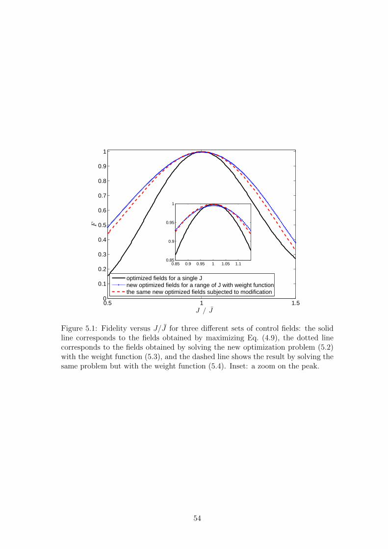
0.5 1 1.50

0.1

0.2

0.3

0.4

0.5

0.6

0.7

0.8

0.9

1

J / J

F

optimized fields for a single Jnew optimized fields for a range of J with weight functionthe same new optimized fields subjected to modification

0.85 0.9 0.95 1 1.05 1.10.85

0.9

0.95

1

Figure 5.1: Fidelity versus J/J for three different sets of control fields: the solidline corresponds to the fields obtained by maximizing Eq. (4.9), the dotted linecorresponds to the fields obtained by solving the new optimization problem (5.2)with the weight function (5.3), and the dashed line shows the result by solving thesame problem but with the weight function (5.4). Inset: a zoom on the peak.

54

fidelities in the vicinity of J/J = 1 but larger in other points.

However, it is possible to improve the fidelities in the vicinity of J/J = 1,

for this new set of optimal fields. We set the weight function as

w(J) = F (u0, J)−1, (5.4)

where u0 is the set of new optimal fields, i.e., the global solution of the prob-

lem (5.2) with the weight function (5.3). The dashed line in Figure 5.1 shows the

corresponding fidelity versus J/J for such set of fields with δJ = 0.1J and the

initial guess equal to u0. The solid line in Figure 5.1 corresponds to the fields

obtained by maximizing Eq. (4.9).

In the next section we analyze the performance of the new sets of control

fields obtained here in the presence of imperfections.

5.2 Performance of the New Optimized Sets of Control Fields

In section 4.4 we analyzed the effect of the static imperfection on the fidelity

of the Toffoli gate. Having used the same method, In this section we show how the

static imperfection affects the fidelity of the gate implemented by the new sets of

control fields obtained in section 5.1. In the other words we analyze the robustness

of the control fields obtained by optimizing the weighted average fidelity in the

presence of static imperfection.

Considering Figure 5.1, we see that the dotted line has the best worst case

performance having the largest values at the boundaries J/J = 0.5, 1.5. However,

in the narrower interval [0.9, 1.1]J the dotted line and the dashed line have almost

the same worst case performance but the dashed line is above the dotted line in

a larger part of the interval. As described below, among the three sets of control

fields discussed here, the dashed line corresponds to the fields that have the best

performance in systems with static disorder less than 10%.

The performance of our new sets of control fields in the presence of noise can

be analyzed in the same way of section 4.4. In the case of static imperfections,

55

the result for the fields optimized according to problem (5.2) with the weight func-

tion (5.3) is shown by dotted line in Figure 5.2. The dashed line in the same

figure shows the situation for the fields optimized with the weight function (5.4).

Specially, for 10% disorder (δ = 0.1) the corresponding fidelities are 98.47% and

98.67%, respectively, showing 0.64% improvement in the first case and 0.84% im-

provement in the second case, comparing to 97.83% [original problem (5.1)]. The

solid line in Figure 5.2 corresponds to the fields obtained in the original prob-

lem (5.1) that is the result from section 4.4 repeated here.

For the dynamical-imperfections case, when the noise frequency is high, the

resulting plots for the three sets of control fields remain almost the same because

the effect of control pulses plays no role in high noise frequencies. However, for low

noise frequencies tgfc = 5, 2, 1 (see section 4.3) the new sets of fields have better

performances.

5.3 Stable Toffoli Gate under the Influence of Static Imperfection

In section 5.1, we obtained two new sets of control fields that realize the

Toffoli gate with improved average fidelity in the presence of imperfection in the

system. The new sets of control fields, comparing to the original set, have more

smooth fidelities around the perfect coupling value J/J = 1 (see Figure 5.1).

However, the fidelities can not be completely flat around J/J = 1. In this section,

we modify the original objective functional in a way to obtain a set of control fields

having almost fixed fidelity in the interval |J/J − 1| ≤ 0.1.

The desired optimization problem can be written as

maxu α(F (u, J − J0) + F (u, J) + F (u, J + J0)

)− β

∣∣ 2F (u, J)− F (u, J − J0)− F (u, J + J0)∣∣

− γ∣∣ F (u, J − J0)− F (u, J + J0)

∣∣ , (5.5)

where α, β and γ are some positive constants and J0 is a point different from

56

J . The first term in the optimization problem (5.5) causes the optimized solution

has high fidelities in the central point J as well as the end points J ± J0. The

second term, the sum of distances between the fidelity at the central point and the

end points, forces the optimized solution to have a smooth fidelity in the interval

[−J0, J0]. Finally, the last term causes the solution has equal fidelities at the end

points.

The solid line in Figure 5.3 shows the fidelity in terms of J/J for the fields

correspond to the global solution of the optimization problem (5.5) with α = 1,

β = 10, γ = 10 and J0 = 0.1J . The set of control fields has been obtained by

performing the optimization process over 200 random initial guesses. The corre-

sponding fidelities in the interval |J/J − 1| ≤ 0.1 vary in the range [0.918, 0.919].

The results from the optimizations problem (5.2) with the weight func-

tions (5.3) and (5.4) have also been depicted in Figure 5.3 for comparison. If

the set of control fields with the flat fidelity in the interval |J/J − 1| ≤ 0.1 is

applied to an imperfect system that has inaccuracy not larger than 10% on the

value of J , the fidelity is remained almost constant for any value of imperfection

in the interval 0 ≤ δ ≤ 0.1. Hence, although such a set of control fields has not

large fidelities at |J/J − 1| ≤ 0.1 it can be considered as a stable realization of the

Toffoli gate that is not sensitive to the imperfect parameter.

5.4 Summary and Conclusions

In this chapter, we modified the optimization problem discussed in chapter 4

to obtain new solutions that are more robust in the presence of noise. By optimizing

the average fidelity with some special weigh functions, Eqs. (5.3) and (5.4), we

obtained new sets of control fields that lead to higher average fidelities in the case

of static imperfections. As discussed in chapter 4, the static imperfection with

half-width less than 10% half-width causes the average fidelity decrease by 2%.

However, the same noise decreases the average fidelities of the new sets of control

fields by less than 1.4% and 1.2% in each case, respectively.

57

Moreover, we obtained another set of control fields that is almost insensitive

to static imperfection when the half-width is less than 10%.

Like chapter 4, the results in this chapter are also valid under the two-

level approximation, i.e., in the absence of a significant leakage from the two-

state computational subspace of the transmon qubits. However, the parameter

imperfections studied here can likely be incorporated in an analogous fashion within

a more complete multi-level analysis.

The results in Sections 5.1 and 5.2 have been also discussed in (Moqadam

et al., 2013) that is recently published in physical review A.

58

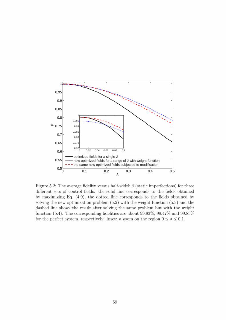
0 0.1 0.2 0.3 0.4 0.50.5

0.55

0.6

0.65

0.7

0.75

0.8

0.85

0.9

0.95

1

δ

F

optimized fields for a single Jnew optimized fields for a range of J with weight functionthe same new optimized fields subjected to modification

0 0.02 0.04 0.06 0.08 0.10.97

0.975

0.98

0.985

0.99

0.995

1

Figure 5.2: The average fidelity versus half-width δ (static imperfections) for threedifferent sets of control fields: the solid line corresponds to the fields obtainedby maximizing Eq. (4.9), the dotted line corresponds to the fields obtained bysolving the new optimization problem (5.2) with the weight function (5.3) and thedashed line shows the result after solving the same problem but with the weightfunction (5.4). The corresponding fidelities are about 99.83%, 99.47% and 99.83%for the perfect system, respectively. Inset: a zoom on the region 0 ≤ δ ≤ 0.1.

59

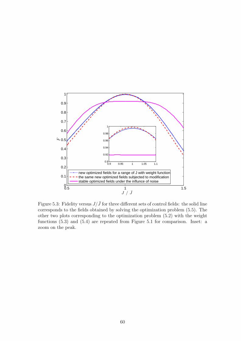
0.5 1 1.50

0.1

0.2

0.3

0.4

0.5

0.6

0.7

0.8

0.9

1

J / J

F

new optimized fields for a range of J with weight functionthe same new optimized fields subjected to modificationstable optimized fields under the influnce of noise

0.9 0.95 1 1.05 1.10.9

0.92

0.94

0.96

0.98

1

Figure 5.3: Fidelity versus J/J for three different sets of control fields: the solid linecorresponds to the fields obtained by solving the optimization problem (5.5). Theother two plots corresponding to the optimization problem (5.2) with the weightfunctions (5.3) and (5.4) are repeated from Figure 5.1 for comparison. Inset: azoom on the peak.

60

Chapter 6

Summary, Conclusions and Future

Works

In this thesis we study the implementation of the Toffoli gate in the sys-

tems with imperfections. The Toffoli gate here is realized through application of

a sequence of microwave control pulses in a chain of three superconducting charge

qubits coupled to a transmission line resonator. For the implementation the trans-

mon qubits have been considered because they are more resistant to the charge

noise and have sufficiently large coherence time to realize the gate. The fidelity of

the gate in the ideal case is about 99.8%. However, due to the imperfections the

fidelity is decreased. We also calculate a new set of microwave control pulses that

not only have the same fidelity in the ideal case but also they are more robust to

the noise and show an improved performance in the presence of noise.

To simulate the imperfection we introduce the noise in the interqubit interac-

tions in the system. In this way, the coupling values no longer remain fixed hence

randomly changes during the time. In the dynamical case, a nonzero frequency is

associated to the noise with which the noise realization is changed. We analyze

the performance of the set of control pulses that are optimized for the ideal case.

To do so, we consider different values for the noise frequency as well as a range of

values for the standard deviation of the noise distribution.

According to the numerical simulations, for every value of the noise frequency,

the average fidelity of the Toffoli gate is decreased when the standard deviation is

61

increased. This is in accordance with our intuition about the decoherence over the

coherent evolution.

For a fixed value of the standard deviation, the high frequency noises are

less dangerous to the system because they generate less decoherence. Actually,

when the noise frequency is sufficiently high the effects of the noise disappear

and the system dynamics would be similar to the ideal case. Such a behavior

can be explained by looking at the noise model that is considered here. The

power spectral density when the frequency approaches infinity goes to zero for all

frequency components. A more detailed analysis using the law of large numbers

shows how the noisy part of the Hamiltonian disappears in the time evolution of

the system. Moreover, using the central limit theorem for large but finite noise

frequencies shows that how the noise affects the fidelity in each control time interval

hence reduces the fidelity.

However, for a fixed value of the standard deviation, the descent of the av-

erage fidelity is continued until the noise period becomes 1/5 of the gate time. for

noise periods larger than that the average fidelity starts to increase. Considering

that the control fields are applied with the period 1/20 of the gate time, we fig-

ure out that when the control-field frequency is sufficiently higher than the noise

frequency the system is protected against the noise similar to the phenomena of

dynamical decoupling.

We also discuss the cases more than one source of noise is introduced to the

system. The noise may be appeared independently between the different interqubit

couplings and also may be affected independently the coupling values in different

directions. However, considering that in our noise model the dynamics of the all

noise parameters are similar, the average fidelity dynamics in these cases remain

qualitatively similar to the case of single noise source. The average fidelity curves

in these cases just decrease faster.

We obtain the average fidelity curves for different values of the noise frequen-

cies for some large values of the standard deviation. Although, as far as we have

62

simulated, there is no universal value for the fidelities in large standard deviations

they remain close to the theoretical value of the full randomizing map saturation

value.

After studying the effects of the dynamical noises we also consider the case of

static noise. In this case, the noise period is much larger than the gate implemen-

tation time. It is associated with a fixed noise in the system. The static noise does

not introduce decoherence to the system but does produce error. Using a uniform

distribution for the noise it is shown that the average fidelity decreases 2%, when

the noise level is less than 10%. Such level of noise is unavoidable in systems that

are consisting of superconducting qubits and microwave resonators.

We also use the quantum control techniques to find new sets of control pulses

that implement the Toffoli gate with an improved performance in the systems with

imperfections. Starting with optimizing a weighted average of the fidelity we obtain

a new set of control fields for which the descent of the average fidelity is 1.36%

for 10% of the noise level. The new obtained set of control fields has however less

fidelity in the ideal case comparing to the original set of fields.

Using an appropriate weight function, we optimize the new set of control

fields to obtain another set with high fidelity performance in the ideal case as well.

The descent of the average fidelity for this latter set is 1.16%.

Finally, by manipulating the objective functional we find an special set of

control fields that is almost insensitive to the noise with half-width less than 10%.

The techniques used in this work may be applied to other multi-qubit gates

as well. Specifically, the 2% reduction of the average fidelity could be expected to

be also valid for other relevant gates, at least for other three-qubit gates, when the

system is affected by a uniform noise with half-width less than 10%.

Moreover, applying the same noise model in a system Hamiltonian written

for multi-level qubits (qudits) it is possible to study the effects of the leakage to

the higher levels in the system.

Our techniques are also applicable in the problems of pure state controlla-

63

bility. In this way, it is possible to find the fidelity of the quantum algorithms as

well. It may be mentioned that in the quantum algorithms both the operator and

state controllability may be used.

We have considered independent distributions in different time intervals for

random variables in the noise model Eq. (4.11). It is possible to extend this method

simulating other types of noise by considering various dependencies between the

random variables in different times. Consequently, the average fidelity may be

improved in a more effective way having those sorts of dependencies. As we have

experimented, using 1/f noise instead of Gaussian noise in different time intervals

leads to different behavior of the average fidelity. In this case increasing the noise

does not reduces the decoherence. Such situation with 1/f noise may be analyzed

as well.

64

Bibliography

Adriano Barenco, Charles H. Bennett, Richard Cleve, David P. DiVincenzo, Nor-

man Margolus, Peter Shor, Tycho Sleator, John A. Smolin, and Harald Wein-

furter. Elementary gates for quantum computation. Phys. Rev. A, 52:3457,

1995.

Alexandre Blais, Jay Gambetta, A. Wallraff, D. I. Schuster, S. M. Girvin, M. H.

Devoret, and R. J. Schoelkopf. Quantum-information processing with circuit

quantum electrodynamics. Phys. Rev. A, 75:032329, 2007.

Alexandre Blais, Ren-Shou Huang, Andreas Wallraff, SM Girvin, and

RJ Schoelkopf. Cavity quantum electrodynamics for superconducting electri-

cal circuits: An architecture for quantum computation. Physical Review A,

69(6):062320, 2004.

Y.I. Bogdanov, A.Y. Chernyavskiy, A. Holevo, VF Lukichev, and AA Orlikovsky.

Modeling of quantum noise and the quality of hardware components of quan-

tum computers. In: International Conference on Micro-and Nano-

Electronics 2012, pagina 87001A. International Society for Optics and Pho-

tonics, 2013.

Constantin Brif, Raj Chakrabarti, and Herschel Rabitz. Control of quantum phe-

nomena: past, present and future. New Journal of Physics, 12(7):075008,

2010.

Ai Min Chen, Sam Young Cho, and Mun Dae Kim. Implementation of a three-

qubit Toffoli gate in a single step. Phys. Rev. A, 85:032326, 2012.

65

John Clarke and Frank K Wilhelm. Superconducting quantum bits. Nature, 453

(7198):1031, 2008.

Domenico d’Alessandro. Introduction to quantum control and dynamics.

Chapman and Hall/CRC,Boca Raton, FL, 2008.

L DiCarlo, JM Chow, JM Gambetta, Lev S Bishop, BR Johnson, DI Schuster,

J Majer, A Blais, L Frunzio, SM Girvin, et al. Demonstration of two-qubit

algorithms with a superconducting quantum processor. Nature, 460(7252):240,

2009.

L DiCarlo, MD Reed, L Sun, BR Johnson, JM Chow, JM Gambetta, L Frunzio,

SM Girvin, MH Devoret, and RJ Schoelkopf. Preparation and measurement of

three-qubit entanglement in a superconducting circuit. Nature, 467(7315):574,

2010.

David P DiVincenzo et al. The physical implementation of quantum computation.

arXiv preprint quant-ph/0002077, 2000.

Paolo Facchi, Simone Montangero, Rosario Fazio, and Saverio Pascazio. Dynamical

imperfections in quantum computers. Phys. Rev. A, 71:060306, 2005.

A. Fedorov, L. Steffen, M. Baur, MP da Silva, and A. Wallraff. Implementation of

a Toffoli gate with superconducting circuits. Nature, 481(7380):170, 2011.

Arkady Fedorov, Lars Steffen, Matthias Baur, MP da Silva, and Andreas Wallraff.

Implementation of a Toffoli gate with superconducting circuits. Nature, 481

(7380):170, 2012.

B. Georgeot and D. L. Shepelyansky. Emergence of quantum chaos in the quantum

computer core and how to manage it. Phys. Rev. E, 62:6366, 2000a.

B. Georgeot and D. L. Shepelyansky. Quantum chaos border for quantum com-

puting. Phys. Rev. E, 62:3504, 2000b.

66

Todd Green, Hermann Uys, and Michael J. Biercuk. High-Order Noise Filtering

in Nontrivial Quantum Logic Gates. Phys. Rev. Lett., 109:020501, 2012.

Aram W. Harrow and Michael A. Nielsen. Robustness of quantum gates in the

presence of noise. Phys. Rev. A, 68:012308, 2003.

R. Heule, C. Bruder, D. Burgarth, and V.M. Stojanovic. Controlling qubit arrays

with anisotropic XXZ Heisenberg interaction by acting on a single qubit. The

European Physical Journal D-Atomic, Molecular, Optical and Plasma

Physics, 63(1):41, 2011.

Rahel Heule, C. Bruder, Daniel Burgarth, and Vladimir M. Stojanovic. Local

quantum control of Heisenberg spin chains. Phys. Rev. A, 82:052333, 2010.

Ryszard Horodecki, Pawe l Horodecki, Micha l Horodecki, and Karol Horodecki.

Quantum entanglement. Rev. Mod. Phys., 81:865, 2009.

Xuedong Hu and S. Das Sarma. Gate errors in solid-state quantum-computer

architectures. Phys. Rev. A, 66:012312, 2002.

Jens Koch, Terri M. Yu, Jay Gambetta, A. A. Houck, D. I. Schuster, J. Majer,

Alexandre Blais, M. H. Devoret, S. M. Girvin, and R. J. Schoelkopf. Charge-

insensitive qubit design derived from the Cooper pair box. Phys. Rev. A, 76:

042319, 2007.

Peter Lambropoulos and David Petrosyan. Fundamentals of quantum optics

and quantum information. Springer, 2007.

Michel Le Bellac. A short introduction to quantum information and quan-

tum computation. Cambridge university press, 2006.

D.A. Lidar. Review of Decoherence Free Subspaces, Noiseless Subsystems, and

Dynamical Decoupling. arXiv preprint arXiv:1208.5791, 2012.

67

S. Machnes, U. Sander, S. J. Glaser, P. de Fouquieres, A. Gruslys, S. Schirmer, and

T. Schulte-Herbruggen. Comparing, optimizing, and benchmarking quantum-

control algorithms in a unifying programming framework. Phys. Rev. A, 84:

022305, 2011.

J Majer, JM Chow, JM Gambetta, Jens Koch, BR Johnson, JA Schreier, L Frunzio,

DI Schuster, AA Houck, A Wallraff, et al. Coupling superconducting qubits via

a cavity bus. Nature, 449(7161):443, 2007.

Yuriy Makhlin, Gerd Schon, and Alexander Shnirman. Quantum-state engineering

with Josephson-junction devices. Rev. Mod. Phys., 73:357, 2001.

Simone Montangero, Giuliano Benenti, and Rosario Fazio. Dynamics of Entan-

glement in Quantum Computers with Imperfections. Phys. Rev. Lett., 91:

187901, 2003.

Simone Montangero and Lorenza Viola. Multipartite entanglement generation and

fidelity decay in disordered qubit systems. Phys. Rev. A, 73:040302, 2006.

T. Monz, K. Kim, W. Hansel, M. Riebe, A. S. Villar, P. Schindler, M. Chwalla,

M. Hennrich, and R. Blatt. Realization of the Quantum Toffoli Gate with

Trapped Ions. Phys. Rev. Lett., 102:040501, 2009.

Jalil Khatibi Moqadam, Renato Portugal, Nami Fux Svaiter, and Gilberto

de Oliveira Correa. Analyzing the Toffoli gate in disordered circuit QED. Phys.

Rev. A, 87:042324, 2013.

Michael A Nielsen and Isaac L Chuang. Quantum computation and quantum

information. Cambridge university press, 2010.

Jorge Nocedal and Stephen J Wright. Numerical optimization. Springer, New

York, 2nd edition, 2006.

E. Paladino, A. D’Arrigo, A. Mastellone, and G. Falci. Decoherence times of

68

universal two-qubit gates in the presence of broad-band noise. New Journal

of Physics, 13(9):093037, 2011.

MD Reed, L. DiCarlo, SE Nigg, L. Sun, L. Frunzio, SM Girvin, and RJ Schoelkopf.

Realization of three-qubit quantum error correction with superconducting cir-

cuits. Nature, 482(7385):382, 2012a.

MD Reed, L DiCarlo, SE Nigg, L Sun, L Frunzio, SM Girvin, and RJ Schoelkopf.

Realization of three-qubit quantum error correction with superconducting cir-

cuits. Nature, 482:382, 2012b.

RJ Schoelkopf, SM Girvin, et al. Wiring up quantum systems. Nature, 451(7179):

664, 2008.

Vladimir M. Stojanovic, A. Fedorov, A. Wallraff, and C. Bruder. Quantum-control

approach to realizing a Toffoli gate in circuit QED. Phys. Rev. B, 85:054504,

2012.

Philipp Strack and Subir Sachdev. Dicke Quantum Spin Glass of Atoms and

Photons. Phys. Rev. Lett., 107:277202, 2011.

D.I. Tsomokos, S. Ashhab, and F. Nori. Fully connected network of superconduct-

ing qubits in a cavity. New Journal of Physics, 10(11):113020, 2008.

DI Tsomokos, MJ Hartmann, SF Huelga, and MB Plenio. Entanglement dynamics

in chains of qubits with noise and disorder. New Journal of Physics, 9(3):79,

2007.

Vlatko Vedral. Introduction to Quantum Information Science (Oxford

Graduate Texts). Oxford University Press, Inc., 2006.

Lorenza Viola, Emanuel Knill, and Seth Lloyd. Dynamical Decoupling of Open

Quantum Systems. Phys. Rev. Lett., 82:2417, 1999.

JQ You and Franco Nori. Atomic physics and quantum optics using superconduct-

ing circuits. Nature, 474(7353):589, 2011.

69