Imaging - run.unl.pt

Supervisor: Prof. Raquel Conceição, Assistant professor, Faculdade

de Ciências, Universidade de Lisboa, Investigadora do

Instituto de Biofísica e Engenharia Biomédica.

So-supervisor: Prof. Ricardo Vigário, Associate Professor, Faculdade de

Ciências e Tecnologia, Universidade Nova de Lisboa.

Miguel Ângelo Borlão Rodrigues

[Nome completo do autor]







Bachelor of Science in Biomedical Engineering

[Habilitações Académicas]







March, 2021

Classifying Breast Tumors using Medical Microwave Radar

Imaging

Título da Tese]

[Título da Tese]

Dissertation submitted in partial fulfillment

of the requirements for the degree of

Master of Science in

Biomedical Engineering

Dissertação para obtenção do Grau de Mestre em

[Engenharia Informática]

i

Miguel Ângelo Borlão Rodrigues

Bachelor of Science in Biomedical Engineering

Classifying Breast Tumors using Medical Microwave Radar

Imaging

Dissertation submitted in partial fulfillment

of the requirements for the degree of

Master of Science in

Biomedical Engineering

Supervisor: Prof. Raquel Conceição, Assistant professor, Faculdade

de Ciências, Universidade de Lisboa, Investigadora do

Instituto de Biofísica e Engenharia Biomédica.

So-supervisor: Prof. Ricardo Vigário, Associate Professor, Faculdade de

Ciências e Tecnologia, Universidade Nova de Lisboa.

March, 2021

iii

Classifying Breast Tumors using Medical Microwave Radar Imaging

Copyright © Miguel Ângelo Borlão Rodrigues, Faculdade de Ciências e Tecnologia, Universidade Nova

de Lisboa.

A Faculdade de Ciências e Tecnologia e a Universidade Nova de Lisboa têm o direito, perpétuo e sem

limites geográficos, de arquivar e publicar esta dissertação através de exemplares impressos reproduzi-

dos em papel ou de forma digital, ou por qualquer outro meio conhecido ou que venha a ser inventado,

e de a divulgar através de repositórios científicos e de admitir a sua cópia e distribuição com objetivos

educacionais ou de investigação, não comerciais, desde que seja dado crédito ao autor e editor.

v

Agradecimentos

Quero começar por expressar o meu profundo agradecimento pelo apoio que os meus Orienta-

dores, Prof.ª Raquel Conceição e Prof.º Ricardo Vigário, me deram para tornar este trabalho possível.

Particularmente, quero agradecer à Prof.ª Raquel por todo o conhecimento que me transmitiu durante

todo este processo, por toda a disponibilidade que sempre demonstrou, pelo voto de confiança que de-

positou em mim para trabalhar consigo e por toda a simpatia e boa disposição que teve comigo. Não

posso também deixar de agradecer ao Matteo, à Daniela e à Catarina, alunos de Doutoramento da Prof.ª

Raquel, por estarem sempre disponíveis para trocar ideias e pelo apoio, disponibilidade e boa-disposição

que sempre demonstraram. Agradecer profundamente também ao restante staff do Instituto de Biofísica

e Engenharia Biomédica (IBEB).

Agradecer profundamente a todo o corpo docente da FCT NOVA, por tudo o que aprendi nestes

5 anos que vou levar comigo. Em especial, um profundo agradecimento à Coordenadora do meu curso,

a Prof.ª Carla Quintão e a todos os professores com que me cruzei no departamento do meu curso,

Departamento de Física, por tudo o que aprendi convosco tanto a nível intelectual como pessoal.

Agradecer ao curso onde fomos e somos todos por um, Engenharia Biomédica. Onde aprendi

que ninguém fica para trás e onde vai um vão todos. Um especial agradecimento ao Lourenço, ao

António, ao Gato, ao Diogo, ao Eduardo, ao Rui, ao Limpinho, ao Tomás, à Madalena, ao Canelhas, à

Beatriz, à Joana, à Inês e à Carolina por estarem comigo nos momentos que mais me marcaram nestes

5 anos fantásticos.

Por fim, quero agradecer a toda a minha família, porque sem eles não seria quem sou hoje.

Agradecer pelo amor e apoio incondicional dos meus pais, Antónia e Luís, pelas rizadas dos meus ir-

mãos, Rita e Filipe, e pela sabedoria dos meus avós, Lili, Custódia e Rogério.

vii

Abstract

Medical Microwave Imaging (MMI) has been studied in the past years to develop techniques to

detect breast cancer at the earliest stages of development. Particularly, ultra-wideband (UWB) micro-

wave radar imaging systems can detect and classify tumors as benign or malignant since this technique

yields information about the size and shape of tumors. In this study we used this technology to classify

tumors.

The primary goal of this dissertation is two-folded. First, producing breast tumor numerical mod-

els and using them in 2D MMI simulations that recreate the conditions of a UWB microwave radar

imaging system. The breast tumor numerical produced resemble real tumor morphologies since they are

made from breast MRI exams segmentations. Second, the data of the backscattered UWB microwave

signals produced by the MMI simulations was used to classify tumors according to their size and histol-

ogy, which is relevant to assess potential of UWB microwave radar imaging systems as a reliable alter-

native method for the classification of breast tumors in the field of Medical Microwave Imaging. The

Classification Algorithms used in this work were Pseudo Linear Discriminant Analysis (Pseudo-LDA),

Pseudo Quadratic Discriminant Analysis (pseudo-QDA), and k-Nearest Neighbors (KNN), alongside

with a feature extraction algorithm – Principal Component Analysis (PCA).

Keywords: Breast Cancer; Medical Microwave Imaging; UWB Microwave Radar Imaging Sys-

tem; MRI Segmentation; Numerical Models; Classification Algorithms.

ix

Resumo

A Imagem Médica por Microondas (do inglês, MMI) tem sido estudada nos últimos anos de forma

a desenvolver técnicas de deteção do cancro da mama nas primeiras fases de desenvolvimento. Em

particular, os sistemas de imagem de radar por microondas em banda ultralarga (do inglês UWB) podem

detetar e classificar os tumores como benignos ou malignos, uma vez que esta técnica produz informação

sobre o tamanho e a forma dos tumores. Neste estudo, utilizámos esta tecnologia para classificar os

tumores.

A dissertação tem dois objetivos principais. Primeiro, produzir fantomas de tumores mamários e

utilizá-los em simulações de MMI em 2D que recriam as condições de um sistema de imagem de radar

por microondas UWB. Os fantomas numéricos de tumores mamários produzidos possuem morfologias

semelhantes a tumores reais, uma vez que são feitos a partir de segmentações de exames de ressonância

magnética da mama. Em segundo lugar, as reflexões dos sinais de microondas UWB produzidos pelas

simulações de MMI foram utilizados para classificar tumores de acordo com o seu tamanho e histologia,

o que é relevante para avaliar o potencial dos sistemas de imagem de radar por microondas UWB como

um método alternativo e fiável para a classificação de tumores mamários no campo da MMI. Os Algo-

ritmos de Classificação utilizados neste trabalho foram a Pseudo Linear Discriminant Analysis (Pseudo-

LDA), Pseudo Quadratic Discriminant Analysis (pseudo-QDA), e a K-Nearest Neighbors (KNN), jun-

tamente com um algoritmo de extração de features - Análise de Componentes Principais (do inglês

PCA).

Palavras-chave: Cancro da mama; Imagem Médica por Microondas; Sistema de Imagem de Ra-

dar de Microondas UWB; Segmentação por Imagens de Ressonância Magnética; Fantoma Corporal

Numérico; Algoritmos de Classificação.

xi

General Index

Agradecimentos ............................................................................................................................ v

Abstract ....................................................................................................................................... vii

Resumo......................................................................................................................................... ix

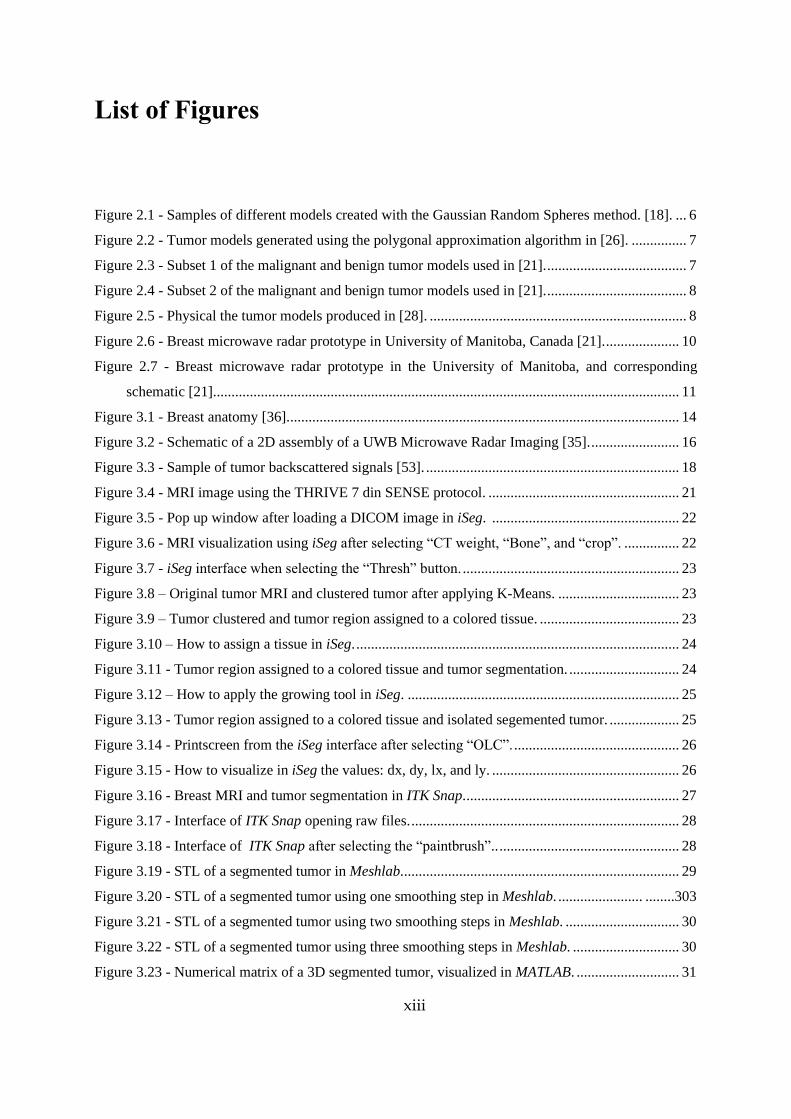
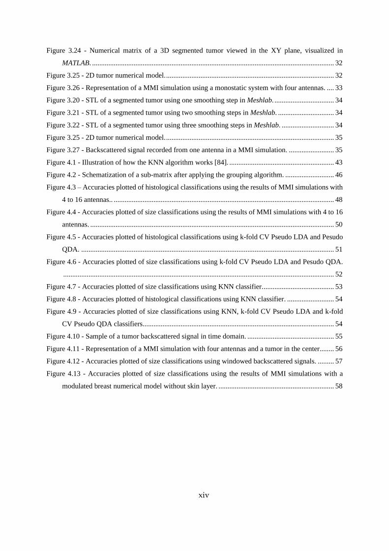
List of Figures ............................................................................................................................ xiii

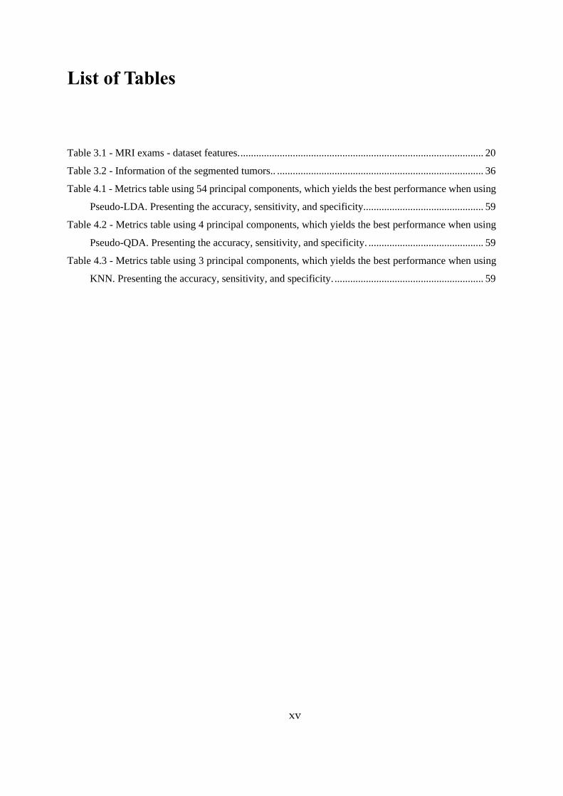
List of Tables .............................................................................................................................. xv

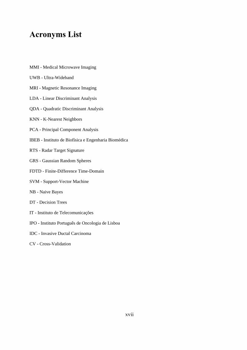
Acronyms List ........................................................................................................................... xvii

1 Introduction ............................................................................................................................ 1

1.1 Motivation and Background .......................................................................................... 1

1.2 Contributions ................................................................................................................. 3

1.3 Dissertation Overview ................................................................................................... 4

2 State of the Art ....................................................................................................................... 5

2.1 Evolution of Tumor Models .......................................................................................... 5

2.2 Classification of Tumors Using Microwave Imaging ................................................... 8

3 Breast Tumor Modelling and Simulations ........................................................................... 13

3.1 Introduction ................................................................................................................. 13

3.2 Background ................................................................................................................. 14

3.2.1 Breast Anatomy .................................................................................................. 14

3.2.2 Breast Tumor ...................................................................................................... 15

3.2.3 Dielectric Properties ........................................................................................... 15

3.2.4 UWB Microwave Radar Imaging ....................................................................... 16

3.2.5 Radar Target Signature – RTS ............................................................................ 17

3.2.6 FDTD Method .................................................................................................... 18

3.3 Materials ...................................................................................................................... 19

3.4 Methodology ............................................................................................................... 20

3.5 Results and Discussion ................................................................................................ 33

3.6 Chapter Conclusions ................................................................................................... 37

4 Breast tumor classification ................................................................................................... 39

4.1 Introduction ................................................................................................................. 39

4.2 Feature Extraction ....................................................................................................... 40

4.2.1 Principal Component Analysis ........................................................................... 40

xii

4.3 Classification ............................................................................................................... 41

4.3.1 Linear Discriminant Analysis and Quadratic Discriminant Analysis ................. 42

4.3.2 K-Nearest Neighbors .......................................................................................... 43

4.4 Methodology ............................................................................................................... 44

4.4.1 Antenna Grouping .............................................................................................. 45

4.4.2 Application of K-fold CV to Pseudo-LDA and Pseudo-QDA ........................... 46

4.4.3 Application of KNN ........................................................................................... 46

4.5 Results and Discussion ................................................................................................ 47

4.5.1 Effect of the number of antennas on the classification accuracy ........................ 47

4.5.2 K-fold Cross-Validation ..................................................................................... 51

4.5.3 k-Nearest Neighbors ........................................................................................... 52

4.5.4 Windowing ......................................................................................................... 55

4.5.5 MMI simulations without simulating skin on the breast model ......................... 57

4.5.6 Metrics ................................................................................................................ 58

4.6 Chapter Conclusions ................................................................................................... 60

5 Conclusion ........................................................................................................................... 63

6 Bibliography ........................................................................................................................ 65

xiii

List of Figures

Figure 2.1 - Samples of different models created with the Gaussian Random Spheres method. [18]. ... 6

Figure 2.2 - Tumor models generated using the polygonal approximation algorithm in [26]. ............... 7

Figure 2.3 - Subset 1 of the malignant and benign tumor models used in [21]. ...................................... 7

Figure 2.4 - Subset 2 of the malignant and benign tumor models used in [21]. ...................................... 8

Figure 2.5 - Physical the tumor models produced in [28]. ...................................................................... 8

Figure 2.6 - Breast microwave radar prototype in University of Manitoba, Canada [21]. .................... 10

Figure 2.7 - Breast microwave radar prototype in the University of Manitoba, and corresponding

schematic [21]. .............................................................................................................................. 11

Figure 3.1 - Breast anatomy [36]. .......................................................................................................... 14

Figure 3.2 - Schematic of a 2D assembly of a UWB Microwave Radar Imaging [35]. ........................ 16

Figure 3.3 - Sample of tumor backscattered signals [53]. ..................................................................... 18

Figure 3.4 - MRI image using the THRIVE 7 din SENSE protocol. .................................................... 21

Figure 3.5 - Pop up window after loading a DICOM image in iSeg. ................................................... 22

Figure 3.6 - MRI visualization using iSeg after selecting “CT weight, “Bone”, and “crop”. ............... 22

Figure 3.7 - iSeg interface when selecting the “Thresh” button. ........................................................... 23

Figure 3.8 – Original tumor MRI and clustered tumor after applying K-Means. ................................. 23

Figure 3.9 – Tumor clustered and tumor region assigned to a colored tissue. ...................................... 23

Figure 3.10 – How to assign a tissue in iSeg. ........................................................................................ 24

Figure 3.11 - Tumor region assigned to a colored tissue and tumor segmentation. .............................. 24

Figure 3.12 – How to apply the growing tool in iSeg. .......................................................................... 25

Figure 3.13 - Tumor region assigned to a colored tissue and isolated segemented tumor. ................... 25

Figure 3.14 - Printscreen from the iSeg interface after selecting “OLC”. ............................................. 26

Figure 3.15 - How to visualize in iSeg the values: dx, dy, lx, and ly. ................................................... 26

Figure 3.16 - Breast MRI and tumor segmentation in ITK Snap. .......................................................... 27

Figure 3.17 - Interface of ITK Snap opening raw files. ......................................................................... 28

Figure 3.18 - Interface of ITK Snap after selecting the “paintbrush”.. ................................................. 28

Figure 3.19 - STL of a segmented tumor in Meshlab. ........................................................................... 29

Figure 3.20 - STL of a segmented tumor using one smoothing step in Meshlab. ....................... ........303

Figure 3.21 - STL of a segmented tumor using two smoothing steps in Meshlab. ............................... 30

Figure 3.22 - STL of a segmented tumor using three smoothing steps in Meshlab. ............................. 30

Figure 3.23 - Numerical matrix of a 3D segmented tumor, visualized in MATLAB. ............................ 31

xiv

Figure 3.24 - Numerical matrix of a 3D segmented tumor viewed in the XY plane, visualized in

MATLAB. ...................................................................................................................................... 32

Figure 3.25 - 2D tumor numerical model. ............................................................................................. 32

Figure 3.26 - Representation of a MMI simulation using a monostatic system with four antennas. .... 33

Figure 3.20 - STL of a segmented tumor using one smoothing step in Meshlab. ................................. 34

Figure 3.21 - STL of a segmented tumor using two smoothing steps in Meshlab. ............................... 34

Figure 3.22 - STL of a segmented tumor using three smoothing steps in Meshlab. ............................. 34

Figure 3.25 - 2D tumor numerical model. ............................................................................................. 35

Figure 3.27 - Backscattered signal recorded from one antenna in a MMI simulation. ......................... 35

Figure 4.1 - Illustration of how the KNN algorithm works [84]. .......................................................... 43

Figure 4.2 - Schematization of a sub-matrix after applying the grouping algorithm. ........................... 46

Figure 4.3 – Accuracies plotted of histological classifications using the results of MMI simulations with

4 to 16 antennas.. .......................................................................................................................... 48

Figure 4.4 - Accuracies plotted of size classifications using the results of MMI simulations with 4 to 16

antennas. ....................................................................................................................................... 50

Figure 4.5 - Accuracies plotted of histological classifications using k-fold CV Pseudo LDA and Pesudo

QDA. ............................................................................................................................................ 51

Figure 4.6 - Accuracies plotted of size classifications using k-fold CV Pseudo LDA and Pesudo QDA.

...................................................................................................................................................... 52

Figure 4.7 - Accuracies plotted of size classifications using KNN classifier. ....................................... 53

Figure 4.8 - Accuracies plotted of histological classifications using KNN classifier. .......................... 54

Figure 4.9 - Accuracies plotted of size classifications using KNN, k-fold CV Pseudo LDA and k-fold

CV Pseudo QDA classifiers.......................................................................................................... 54

Figure 4.10 - Sample of a tumor backscattered signal in time domain. ................................................ 55

Figure 4.11 - Representation of a MMI simulation with four antennas and a tumor in the center........ 56

Figure 4.12 - Accuracies plotted of size classifications using windowed backscattered signals. ......... 57

Figure 4.13 - Accuracies plotted of size classifications using the results of MMI simulations with a

modulated breast numerical model without skin layer. ................................................................ 58

xv

List of Tables

Table 3.1 - MRI exams - dataset features. ............................................................................................. 20

Table 3.2 - Information of the segmented tumors.. ............................................................................... 36

Table 4.1 - Metrics table using 54 principal components, which yields the best performance when using

Pseudo-LDA. Presenting the accuracy, sensitivity, and specificity.............................................. 59


Pseudo-QDA. Presenting the accuracy, sensitivity, and specificity. ............................................ 59


KNN. Presenting the accuracy, sensitivity, and specificity. ......................................................... 59

xvii

Acronyms List

MMI - Medical Microwave Imaging

UWB - Ultra-Wideband

MRI - Magnetic Resonance Imaging

LDA - Linear Discriminant Analysis

QDA - Quadratic Discriminant Analysis

KNN - K-Nearest Neighbors

PCA - Principal Component Analysis

IBEB - Instituto de Biofísica e Engenharia Biomédica

RTS - Radar Target Signature

GRS - Gaussian Random Spheres

FDTD - Finite-Difference Time-Domain

SVM - Support-Vector Machine

NB - Naive Bayes

DT - Decision Trees

IT - Instituto de Telecomunicações

IPO - Instituto Português de Oncologia de Lisboa

IDC - Invasive Ductal Carcinoma

CV - Cross-Validation

1

1 Introduction

1.1 Motivation and Background

Worldwide in 2018, there were approximately 18 million new cancer cases. Breast cancer ac-

counted for 12.26% of cases, only surpassed by lung cancer with 12.29% cases [1]. Among women,

breast cancer is the most common malignant tumor. It is estimated that one in eight to ten females will

develop the pathology. Even though the mortality rate is dropping in developed countries due to earlier

detection and more effective therapeutics, the goal to improve the survival rate and give patients better

life quality is relevant. Besides that, it is necessary to lower the cost of breast tumor diagnostic and

therapeutic methods to help developing countries, where this type of tumor is the deadliest [2].

In Portugal, according to the last report of the International Agency for Research on Cancer, in

2020 alone, breast tumor was the most incident type of cancer with 7041 new cases and 1864 deaths.

Accounting for 11.6% of all new cancer cases and 6.2% of deaths from cancer. The mortality numbers

place breast cancer in the fifth position overall, but among women, it is the deadliest [3].

One of the most critical keys to increase patients' quality of life and their survival rates is detecting

breast tumors in its early stages of development. Hence tumor diagnostic techniques are fundamental.

Over the last years, medical imaging techniques have been the primary source of breast tumor detection

and classification. The most common imaging techniques in breast tumor are X-ray mammography,

ultrasound imaging, and magnetic resonance imaging (MRI).

X-ray mammography uses low doses of ionizing radiation to penetrate a compressed breast to

obtain an image. It can detect breast cancer early. There is evidence that mammography screened pop-

ulations have lower mortality rates and higher quality of life since early staged cancer has less invasive

treatments [4]. Another feature that incentives its worldwide use is the low-cost associated. However, it

also has drawbacks, such as considerable high rates of false-positive and false-negative results, espe-

cially in dense breasts [5]. False-positive happens when a patient is diagnosed with breast cancer when

it is not present, causing unnecessary new exams and possibly even treatments, leading to stress and

lowering the quality of life of the patient [5]. False-negative is a false result of an absence tumor when

it is present, leading to possible development of the cancer, which may lower the chances of curing it

[4]. Besides that, since the exam uses ionizing radiation, there is rare probability to develop cancer [6],

2

this has a direct consequence disallowing pregnant women to take this type of exam. The procedure can

also be painful and stressful due to the compression of the breast.

There are also non-ionizing detection methods, such as ultrasound and MRI, to be used as com-

plementary exams with mammographies. In two situations, when needed to assess whether a detected

tumor by mammography is malignant or not, and when the breasts are too dense, not allowing X-ray

penetration [7]–[9].

Ultrasound is based on the transmission of high-frequency sound waves and the respective re-

cording of the backscattered signals. Since the reflections have different intensities depending on the

acoustic properties of the tissues under test [10], it allows visualizing muscle, adipose tissues, tumors,

etc. Ultrasound has been used as a complementary tool for mammography when an abnormal change is

detected. Even though it has low resolution and cannot differentiate between benign and malignant small

tumors in most situations, it can distinguish a cyst filled with fluid from a tumor [9]. Another situation

to use ultrasound is when the patient has breast tissue so dense that the x-Rays of the mammography

may not penetrate it. Ultrasound also has the benefits of being low-cost and not using ionizing radiation.

The main limitation of this technique is that it cannot well-differentiate adipose tissue from a tumor, so

it is mainly used after an MRI exam has located the abnormality in study [9].

MRI uses magnetic fields, computer systems, and radio waves to reconstruct 3D images. It is

highly sensitive in detecting invasive and small lesions compared with mammography and ultrasound

techniques. This technique allows the detection of some invasive and noninvasive breast tumors that

could be invisible otherwise. MRI has low specificity meaning it has trouble differentiating benign and

malignant tumors. Therefore, it is mostly used when a biopsy has previously confirmed a malignant

tumor to provide more data about the cancer in study [8], [9]. It can also be used to complement breast

screening with mammography or ultrasound. In cases where the patient is at high risk or has already

been diagnosed with breast tumors, this technique can retrieve the size of the cancer and check the

presence of other tumors within the affected breast or in the opposite breast. Besides low specificity,

MRI has more limitations, such as high costs associated and the long time to take the exam [8], [9].

Due to the disadvantages of the current techniques above, Medical Microwave Imaging (MMI)

appears as a promising alternative because of the potential benefits it may have. This method has a lower

cost than the other mentioned techniques, is not invasive, and is more user-friendly, not requiring breast

compression as in mammography. MMI is less harmful to the patient since it works in a non-ionizing

spectrum, the microwaves [11].

MMI is based on the dielectric contrast between tumor and healthy breast tissues at microwave

frequencies, and its potential to detect breast tumors has been widely investigated. Several research

3

teams have developed breast microwave imaging systems and crossed breakthroughs both in the private

and academic sectors.

Some companies have developed breast cancer MMI detection systems. These include Micrima

based in Bristol, United Kingdom, which developed its equipment called MARIA® [12], and MVG with

Wavelia, in France [13]. In the academic sector, university groups are heading the MMI innovation,

such as Dr. Elise Fear’s research team from the University of Calgary [14], [15] and the Breast Cancer

Detection Research Group led by Milica Popovic at McGill University [16], [17].

Performing trials with microwave imaging systems on patients is required to assess the real po-

tential of the technology. However, they must face strict ethics approval and a large set of volunteers to

participate. Despite the limitations, some companies, including Micrima [12], are already completing

clinical trials. For now, another viable and cheaper way to test and improve breast MMI is using breast

and tumor numerical models, without the high expenses of clinical trials.

This dissertation continues the work described in the State-of-the-Art Chapter, addressing ultra-

wideband (UWB) microwave radar imaging. It might be a potentially useful imaging modality that al-

lows breast tumor diagnoses and data to classify tumors either as benign or malignant. Several studies

[18]-[23] have shown that microwave backscattered signals change in the presence of tumors with dif-

ferent sizes and morphologies within the breasts. These studies presented evidence that classification

algorithms can indeed reliably classify tumors using the backscattered signals.

In this work, the main goal is to produce numerical tumor models from segmenting breast MRI

exams and use them in 2D MMI simulations that recreate the conditions of a UWB microwave radar

imaging prototype system. The data collected was processed and used by classification algorithms to

attempt separating tumors in size and histology, specifically as either an invasive ductal carcinoma or

not. Initially, the tumor models were meant to be 3D printed and tested with a pre-clinical UWB micro-

wave radar imaging prototype. The 2D MMI simulations were the most viable solution to continue this

work considering the restrictions imposed by the covid-19 pandemic.

1.2 Contributions

This work was developed in Instituto de Biofísica e Engenharia Biomédica (IBEB), located in the

Faculdade de Ciências da Universidade de Lisboa. Nowadays, the field of tumor detection and classifi-

cation using medical imaging is searching for alternative techniques to overcome the limitations of the

currently available technology, whose primary goal is to diagnose a patient as soon as possible to max-

imize the probabilities of curing breast cancer. MMI appears as a promising technique, and this disser-

tation produced the following contributions to assess the potential of UWB microwave radar imaging:

4

• Creation of 3D and 2D numerical tumors dataset from segmenting MRI breast exams. The 3D

numerical models are ready to be 3D printed and used in future studies, since they were saved as STLs.

• Tumor size and histological classification using different classification algorithms, including

pseudo-LDA, pseudo-QDA, and KNN, using the data collected from the 2D MMI simulations with the

2D tumor numerical models.

• Inferred the minimum number of principal components required to yield reliable classification

results.

• Assessed the minimum number of antennas required, in the 2D MMI simulations, to collect

enough data to make reliable tumor classifications.

• Since tumor location was known, the data collected from the 2D MMI simulations was win-

dowed to extract only the signal portion belonging to tumor response and assess whether using that

portion alone in the classification systems improves the performance.

• Finally, compared the results of tumor classification using data from MMI simulations with and

without a skin layer on the modulated breast model to evaluate the impact of the skin presence.

1.3 Dissertation Overview

This work is divided into five different chapters. Chapter 1 corresponds to the Introduction. It

details the motivation for the dissertation, giving a background about the impact of breast cancer on

society and breast cancer imagiology techniques to explain MMI potential in this field. The chapter also

includes the contributions that this work produced.

In Chapter 2, the State of the Art shows the evolution of tumor modeling and tumor classification

regarding UWB microwave radar imaging, which is vital to understand what lead to this work.

Both Chapter 3 and Chapter 4 have independent results, discussions, and chapter conclusions.

Chapter 3 gives the background to breast tumors and UWB microwave radar breast imaging. Explains

how tumor models were made through segmenting MRI breast exams. This Chapter also shows how 2D

MMI simulations recreate UWB microwave radar imaging prototypes. Meanwhile, Chapter 4 explains

how the data from the MMI simulations, in Chapter 3, was used to classify the tumor models in size and

histology.

Finally, in Chapter 5, the conclusions of this work are presented, as well as the future work ex-

pected to keep validating MMI as a viable technique to diagnose breast tumors.

5

2 State of the Art

MMI has potential to reliably detect the presence of a tumor due to the dielectric properties con-

trast between breast tumor and the remaining breast tissues. Recent studies about UWB microwave radar

imaging have shown how the Radar Target Signature (RTS) present in the backscattered microwave

signals may provide data about the shape and size of tumors. Since malignant and benign tumors have

different morphologies, this technology can potentially be a reliable way to classify tumors in the future

[18]–[23]. This Chapter presents the state of the artwork in this field. It starts by showing the evolution

in breast tumor modeling, and then it presents studies about the classification of tumors using microwave

imaging.

2.1 Evolution of Tumor Models

Initially, tumor classification studies in MMI began by using mathematical models of tumors that

brought them closer to real tumor shapes, such as the Gaussian Random Spheres (GRS) method. This

model allows creating 3D models of different sizes and shapes and recreating different types of surface

texture. The GRS method follows an algorithm proposed by Muinonen [24]. Each GRS uses spherical

coordinates and has a radius vector 𝑟 = 𝑟(𝜗, 𝜑). The radius vector is defined by the logarithmic radius

𝑠 = 𝑠(𝜗, 𝜑), also using spherical coordinates, both presented in (2.1) and (2.2).

𝑟(𝜗, 𝜑) = 𝛼 . exp[𝑠(𝜗, 𝜑) −

1

2𝛽2] (2.1)

𝑠(𝜗, 𝜑) = ∑ ∑ 𝑠𝑙𝑚𝑌𝑙𝑚

𝑙

𝑚=−𝑙

∞

𝑙=0

(𝜗, 𝜑) (2.2)

Where 𝛼 stands for the mean radius, 𝛽 is the standard deviation of the logarithmic radius, 𝑌𝑙𝑚 are

the orthonormal spherical harmonics, 𝑠𝑙𝑚 are the spherical harmonics weight coefficients, in which l

and m stand for the degree and the order of expansion, respectively [25].

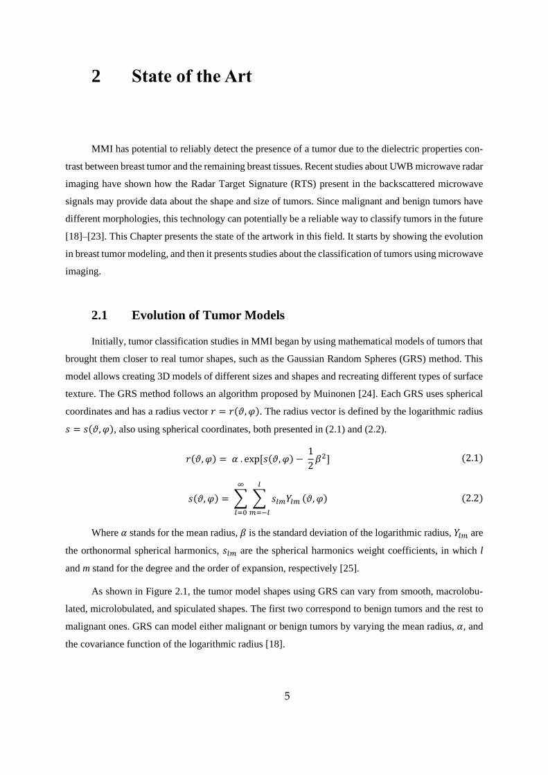
As shown in Figure 2.1, the tumor model shapes using GRS can vary from smooth, macrolobu-

lated, microlobulated, and spiculated shapes. The first two correspond to benign tumors and the rest to

malignant ones. GRS can model either malignant or benign tumors by varying the mean radius, 𝛼, and

the covariance function of the logarithmic radius [18].

6

Figure 2.1 - Samples of different models created with the Gaussian Random Spheres method. Smooth benign

tumors are represented in (a) and macrolobulated benign tumors in (b). Microlobulated malignant tumors are rep-

resented in (c) and spiked malignant tumors in (d) [18].

A Debye model can be used to attribute the dielectric properties of the corresponding biological

tissues . After modeling the tumors, these can be modelled in a Finite-Difference Time-Domain (FDTD)

model where Maxwell's equations are implemented to simulate the electromagnetic behavior of tissues

in the presence of microwave radiation and simulate the radar target signature (RTS) of each tumor, and

use that information to make tumor classifications, following [19] and [20].

In [26], a different method to generate 3D numerical tumor models is proposed. This method

extends the work by Chen et al. in 2008, which generated 2D accurate tumor models using polygonal

approximation [27]. The polygonal approximation is based on the principle that the shape of a tumor

matches an ellipsoid.

𝑑2𝑐𝑜𝑠2𝜗𝑠𝑖𝑛2𝜑

𝑎2+

𝑑2𝑠𝑖𝑛2𝜗𝑠𝑖𝑛2𝜑

𝑏2 +

𝑑2𝑐𝑜𝑠2𝜑

𝑐2= 1 (2.3)

Where d, 𝜗 and 𝜑 are the spherical coordinates that describe the ellipsoid. The variable d corre-

sponds to the distance of each vertex to the center of the ellipsoid, it is a function of the two angles

𝜗 and 𝜑. The values a, b and c prespecify the lengths of each semi-axes.

The extension of the method is applied by adding a new variable. For each vertex of the polygon,

d (𝜗, 𝜑)is modified according to the new variable s, which is a parameter that manages the level of

spiculation at the tumor face.

𝑑′(𝜗, 𝜑) = 𝑛 [𝑑(𝜗, 𝜑) (1 + µ(𝜗, 𝜑))] (2.4)

7

Where µ ∈ U [-s, +s], 𝑑′corresponds to the new distance to the center after applying the described

modification above, and U is the uniform distribution from which s is randomly chosen. The level of

spiculation varies between 0 ≤ s ≤ 1, where s = 0 yields a perfectly smooth border and s = 1 yields the

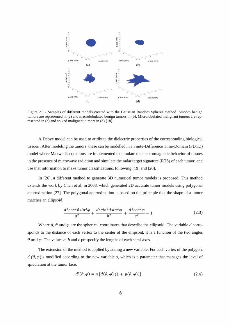
maximum level of spiculation. The parameter n defines the proportion of the surface of the tumor area

covered with spicules. Figure 2.2 shows examples of different numerical tumor models using this

method.

Figure 2.2 - Tumor models generated with the proposed algorithm in [26] for varying sizes, shapes and degrees of

spiculation (s). Mean radii for the models vary between 3 and 10 mm. Degrees of spiculation: (a), (b) s = 0.3; (c)

s = 0.8; (d) s = 0.2 and s = 1.

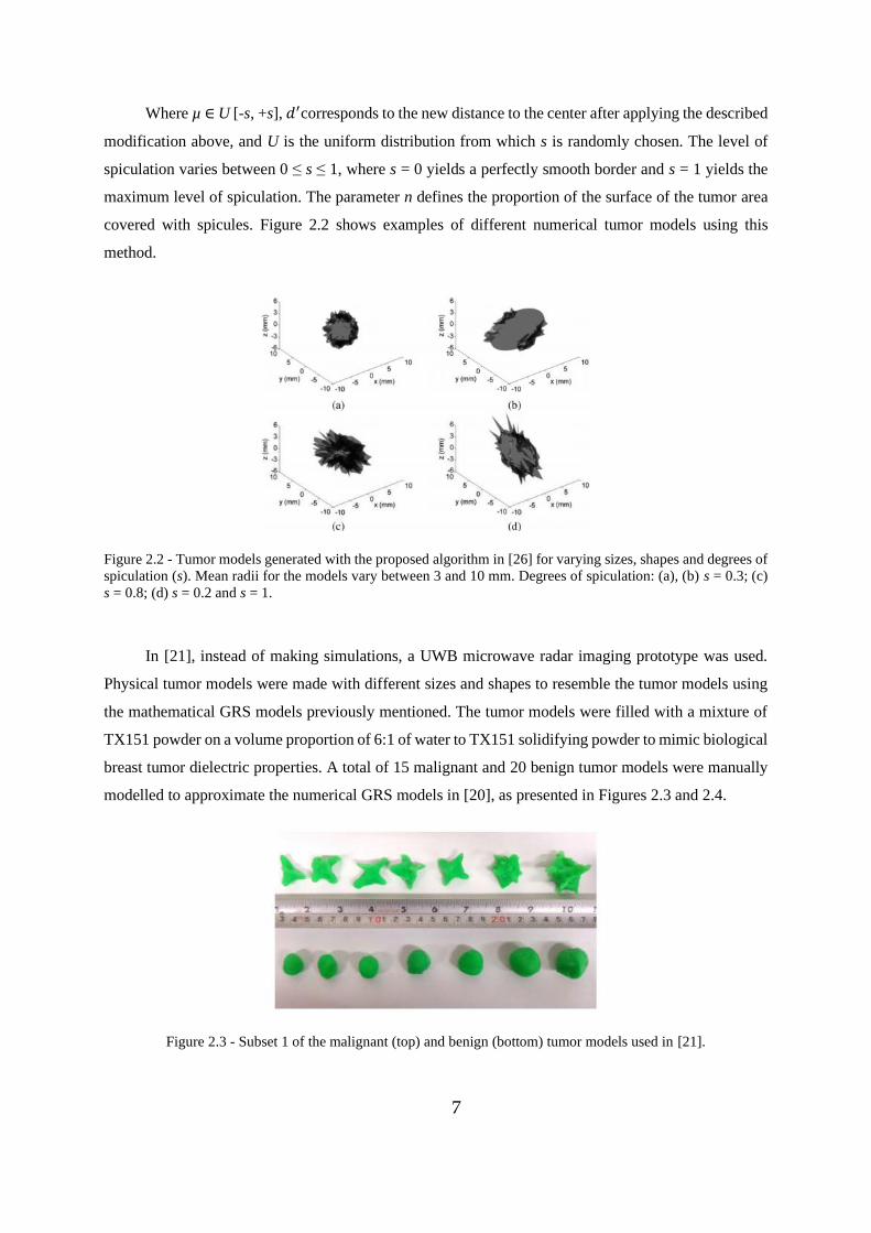
In [21], instead of making simulations, a UWB microwave radar imaging prototype was used.

Physical tumor models were made with different sizes and shapes to resemble the tumor models using

the mathematical GRS models previously mentioned. The tumor models were filled with a mixture of

TX151 powder on a volume proportion of 6:1 of water to TX151 solidifying powder to mimic biological

breast tumor dielectric properties. A total of 15 malignant and 20 benign tumor models were manually

modelled to approximate the numerical GRS models in [20], as presented in Figures 2.3 and 2.4.

Figure 2.3 - Subset 1 of the malignant (top) and benign (bottom) tumor models used in [21].

8

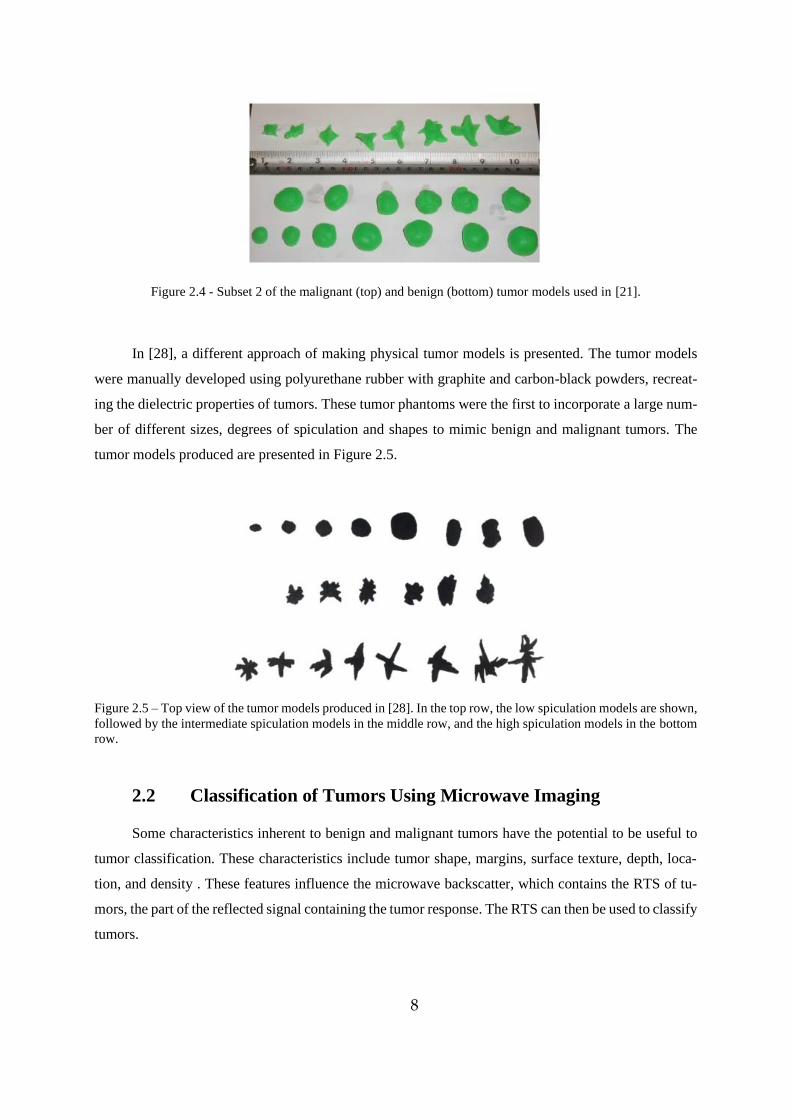
Figure 2.4 - Subset 2 of the malignant (top) and benign (bottom) tumor models used in [21].

In [28], a different approach of making physical tumor models is presented. The tumor models

were manually developed using polyurethane rubber with graphite and carbon-black powders, recreat-

ing the dielectric properties of tumors. These tumor phantoms were the first to incorporate a large num-

ber of different sizes, degrees of spiculation and shapes to mimic benign and malignant tumors. The

tumor models produced are presented in Figure 2.5.

Figure 2.5 – Top view of the tumor models produced in [28]. In the top row, the low spiculation models are shown,

followed by the intermediate spiculation models in the middle row, and the high spiculation models in the bottom

row.

2.2 Classification of Tumors Using Microwave Imaging

Some characteristics inherent to benign and malignant tumors have the potential to be useful to

tumor classification. These characteristics include tumor shape, margins, surface texture, depth, loca-

tion, and density . These features influence the microwave backscatter, which contains the RTS of tu-

mors, the part of the reflected signal containing the tumor response. The RTS can then be used to classify

tumors.

9

In [19] and [20], different tumor classification approaches are performed using the RTS obtained

through 3D MMI simulations that record UWB microwave backscatter signals. These studies use the

GRS method, mentioned before, to model the shape and size of benign and malignant tumor models. A

Debye model was used to model the dielectric properties of biological breast tumors in the models, and

the same for the homogeneous breast models used. The backscattered signals were first processed by

applying a feature extraction algorithm – PCA - to extract the most relevant features (principal compo-

nents) used in the classifications. All three classifiers – Linear Discriminant Analysis (LDA), Quadratic

Discriminant Analysis (QDA), and Support-vector machine (SVM) - were used to assess the size and

shape of the 3D tumor models. A cross-validation method was used in each classification to infer each

classifier performance using a testing set independent from the training set. This study analyzed the

classifiers performances using a set of up to eight multi-stage different classification architectures,

which categorize the data in different levels of granularity in size or shape. For example, classifying the

tumors as benign or malignant and then sub-dividing malignant tumors into spiculated and microlobu-

lated tumors and benign tumors into macrolobulated and smooth tumors. In [19] overall, LDA and QDA

have similar performances when using the same architecture. After comparing the previous LDA and

QDA results with the SVM results in [20], the SVM outperforms both LDA and QDA considering all

architectures used in the studies.

In 2015, the effect of pre-processing signals on diagnostic performance was investigated by iso-

lating the reflected signal through a windowing function, extracting the tumor signature from the signal,

while decreasing the influence of the background [22]. Tumor models of various sizes and shapes were

placed in various positions inside clinical realistic breast models from the UWCEM research group

repository [29]. The classification structure was based on PCA in combination with SVM. In conclusion,

the classification performance increased when the windowing method was applied to the pre-processed

signal in more complex and heterogeneous breast models.

In 2018, Oliveira et al. [23], presented an analysis of machine learning classifying numerical

breast tumor models, using backscattered signals recorded by 12 antennas in a multistatic system, where

all signals were generated in MMI simulations. A comparison between applying and not applying a

tumor windowing approach to extract only the signal tumor response elements of interest from the

backscattered signal was performed, combined with feature extraction. The classification algorithm used

was random forests [30] to distinguish benign and malignant tumors. Antenna grouping was also per-

formed. To better understand antenna grouping results, it is important to define how backscattered sig-

nals are used in the decision-making process. Each recorded signal per receiving antenna is classified

independently. However, in a real scenario, a patient requires a final decision based on the full scan and

not based on each signature collected. Therefore, all independent channel classifications must be com-

bined to make the final classification. The final classification corresponds to the classification of the

10

majority vote. Grouping the antennas predictions was important in disregarding incorrect classifications

from lower quality recorded signals [23].

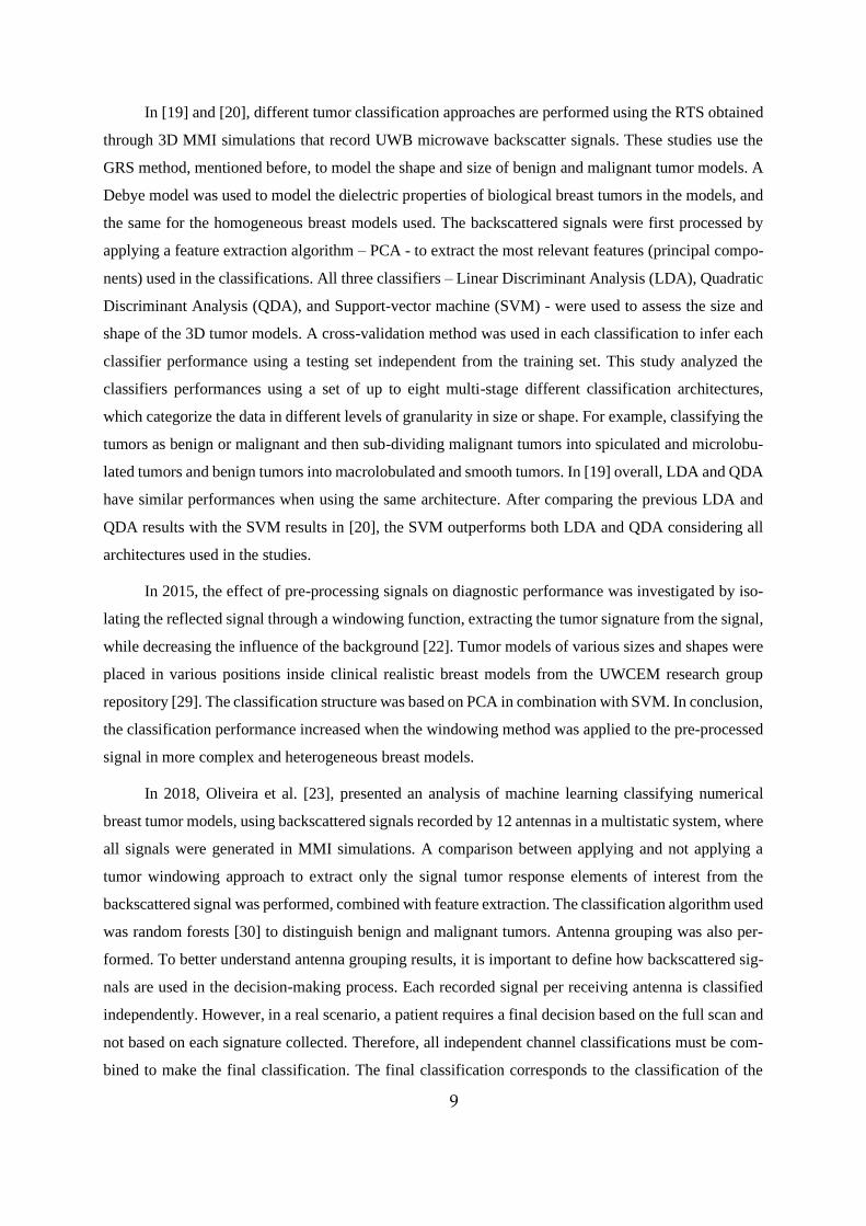
Instead of making MMI simulations, in early 2020, Conceição et al. [21], experiments were per-

formed using a pre-clinical UWB microwave radar imaging prototype at the University of Manitoba

with tumor and breast physical phantoms. A monostatic radar system was used, where a single antenna

emitted a UWB microwave pulse and received the backscattered signal at different angles. These signals

contain the RTS of the tumor, used to classify tumors as benign or malignant.

As presented in Figure 2.6, the antenna of the prototype was immersed with canola oil to mimic

the speed of microwave radiation in breasts. During the recordings, the breast phantom spins so that the

single fixed antenna collects backscatters at different angles [21].

Figure 2.6 - Breast microwave radar prototype in University of Manitoba, Canada: (a) antenna location, (b) step

motor fixed at the center of the tank, (c) tank filled with canola oil [21].

Both homogeneous and heterogeneous breast phantoms were modeled using a styrene-acryloni-

trile cylinder with a diameter and a height equal to 13 cm and 35 cm, respectively. The cylinder was

filled with glycerin, mimicking biological breast tissue dielectric properties. The heterogeneous breast

phantoms also have fibroglangular tissues modeled as a cylinder with a 1.5 cm diameter and 3 cm in

height. The fibroglangular tissues were made of a mixture of TX151 dissolved in water, a volume pro-

portion of 4:1 of water to the solidifying powder, mimicking the milk ducts dielectric properties. Re-

garding the methodology of the tumor phantoms in this study, it was already mentioned in the tumor

11

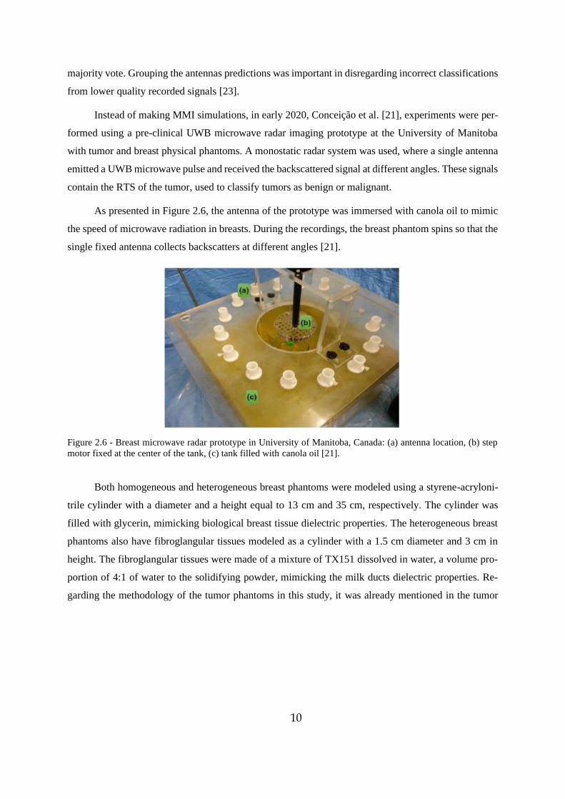
model evolution section. All tumor models were individually tested inside the homogeneous and heter-

ogeneous breast models, as presented in Figure 2.7 [21].

Figure 2.7 - Breast microwave radar prototype in the University of Manitoba (left), and corresponding schematic

(right): view with antenna and heterogeneous breast phantom. Tank filled with canola oil in yellow (e), antenna

on the left and the cylinder breast phantom (a) with two green masses: the tumor on the left (c), closer to the

antenna (b), and a fibroglandular cluster (d) on the right [21].

Breast-tumor pairs were irradiated using the prototype, where a single antenna emitted a UWB

microwave pulse and received the backscattered signal at different angles. Before classification, a fea-

ture extraction algorithm – PCA, was applied to extract the RTS of each tumor from the recorded

backscattered signals [21].

Classifications of tumors as benign or malignant were performed, based only on the RTS of the

tumors inside the breast phantoms. Three machine learning classifiers were used – Naive Bayes (NB),

Decision Trees (DT), and KNN, since they are fast to train and test when compared to SVM, for exam-

ple. An artificial skin response was added to the signals to assess the impact of skin artifacts on the

classifiers performances while directly comparing the records without skin response added. The study

concluded that KNN often outperformed DT and NB classifiers when using either homogeneous or

heterogeneous breast phantoms without skin response. KNN does not require high computational per-

formance like SVM, yet it yields similar good results. Finally, considering an artificial skin response

did not significantly affect the classifications performances since PCA efficiently extracts the tumor

response from the recorded signals [21].

13

3 Breast Tumor Modelling and Simulations

3.1 Introduction

MMI has already been studied with patients [31], [32]. Regarding Micrima [32], the company has

already trialed over 400 patients using their breast cancer detection system – MARIA. Since MMI is

still in development it is relevant to acquire data not only in patients’ trials but also using tumor models

to evaluate the potential and improve this modality. In this work, we proceeded to make 3D and 2D

numerical tumor models as close to their original shape as possible from segmenting breast tumor from

MRI exams and use MMI simulations to numerically recreate a UWB microwave radar imaging system

operating on breast and tumor models, since it models the dielectric properties of breast, skin, and tumor

tissues. The global pandemic caused by covid-19 imposed changes in this work. Initially, the 3D tumor

models were to be 3D printed as a hollow volume to be filled with a mix of TX151 and water that would

mimic the dielectric properties of biological tumors. The physical tumor models were to be tested in a

medical UWB microwave radar imaging prototype at Instituto de Telecomunicações (IT), Instituto Su-

perior Técnico de Lisboa. At the time all 3D numerical tumor models were completed, access to the lab

become limited. The solution to continue the work was to use 2D tumor slices in simulations of the

UWB microwave radar imaging prototype with 2D FDTD modelling. The MATLAB scripts available,

at the time, only allowed 2D FDTD modelling. Besides, making 3D FDTD modelling, using the 3D

tumor models, would require more computational power than available. The contributions in this chapter

are the following:

- Background context to better understand the scope of this work, including breast and breast

tumor anatomy, dielectric properties, UWB microwave radar imaging, radar target signature and FDTD

method.

- Provide a segmentation method that distinguishes breast tissues from existing tumors in MRI

exams to achieve realistic tumor models.

- Demonstrate how to smooth tumor model surfaces, which is vital in low resolution cases.

- All tumor STLs created can be 3D printed and used in future studies with UWB microwave

radar imaging prototypes.

- Recording of backscattered signals from the MMI simulations.

Chapter 2 presented the state of the art. This chapter addresses how it is possible to obtain breast

tumor models from segmenting MRI exams and using them in simulations to recreate the functionality

of a UWB microwave radar imaging prototype.

14

3.2 Background

3.2.1 Breast Anatomy

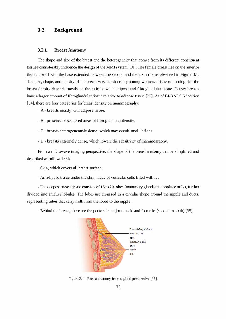
The shape and size of the breast and the heterogeneity that comes from its different constituent

tissues considerably influence the design of the MMI system [18]. The female breast lies on the anterior

thoracic wall with the base extended between the second and the sixth rib, as observed in Figure 3.1.

The size, shape, and density of the breast vary considerably among women. It is worth noting that the

breast density depends mostly on the ratio between adipose and fibroglandular tissue. Denser breasts

have a larger amount of fibroglandular tissue relative to adipose tissue [33]. As of BI-RADS 5th edition

[34], there are four categories for breast density on mammography:

- A - breasts mostly with adipose tissue.

- B - presence of scattered areas of fibroglandular density.

- C - breasts heterogeneously dense, which may occult small lesions.

- D - breasts extremely dense, which lowers the sensitivity of mammography.

From a microwave imaging perspective, the shape of the breast anatomy can be simplified and

described as follows [35]:

- Skin, which covers all breast surface.

- An adipose tissue under the skin, made of vesicular cells filled with fat.

- The deepest breast tissue consists of 15 to 20 lobes (mammary glands that produce milk), further

divided into smaller lobules. The lobes are arranged in a circular shape around the nipple and ducts,

representing tubes that carry milk from the lobes to the nipple.

- Behind the breast, there are the pectoralis major muscle and four ribs (second to sixth) [35].

Figure 3.1 - Breast anatomy from sagittal perspective [36].

15

3.2.2 Breast Tumor

Breast tumor development is different from person to person. However, it is characterized as a

chaotic proliferation of the epithelial cells, which usually begins either in the lobules or the ducts. His-

tologically it is commonly classified as two different main types, invasive or in situ (also known as non-

invasive). Depending on the spread outside the place they first started. In situ tumors remain in their

original site, usually either in the ducts or lobules of the breast. Conversely, invasive cancers spread into

the surrounding healthy tissues [35], [37], [38].

Most breast tumors can be sub-classified from invasive and in situ into the following [35]:

- Invasive ductal carcinoma is the most common breast cancer (70 to 80% of breast tumor cases)

and occurs in the cells lining breast ducts.

- Invasive lobular carcinoma represents about 10% of breast tumors and occurs in the lobules of

the breasts.

- Ductal carcinoma in situ is a type of tumor where cells are found within the ducts without mi-

gration to other tissues.

- Lobular carcinoma in situ is not a kind of cancer; however, its presence increases cancer risk

[35].

3.2.3 Dielectric Properties

Mainly, two dielectric properties express the interaction between the breast tissues and the elec-

trical field applied during MMI: the relative permittivity and conductivity [39]. The membrane of tumor

cells is different from healthy tissues, which leads to a different membrane permeability, affecting the

regulatory process of osmosis. Higher membrane permeability makes the tumor tissues retain more fluid

than normal cells. In the form of water, the extra fluid alters the tissues dielectric properties [35]. High

water content tissues, such as tumors, have both higher relative permittivity and conductivity than low

water content tissues, like, for example, breast fat [35].

Given that most of the breast tissues have low water content, this creates a dielectric contrast in

the presence of higher water concentrated tissues like breast tumors. Additionally, the extra quantity of

sodium ions within tumor tissues also contributes to higher dielectric properties compared to healthy

breast tissues [35]. These properties affect the phase, attenuation, transmission, and reflection of UWB

signals through the breast [40]. At the microwave spectrum range, higher conductivity means an in-

creased absorption and, consequently, attenuation of signals that travel through tissues with those prop-

erties. Considering the breast, microwave signals have significant penetration since breast tissues have

low water content. In the presence of a tumor, the microwaves have more interactions with these high-

16

water content tissues, leading to a more energy attenuation in that region and producing more reflections,

which can be detected outside the breast [41].

3.2.4 UWB Microwave Radar Imaging

Microwaves are part of the radiation spectrum in the range of frequencies between 300MHz and

300GHz. Although, it is worth noting that the range of frequencies for biomedical imaging applications

does not exceed 30 GHz, this range offers patient safety, and balances spatial resolution and penetration

depth [42], [43].

MMI aims to detect tumors using microwaves and is based on the dielectric properties differences

between healthy breast tissues and tumors in this spectrum of radiation, as previously described. There

are different breast image approaches in MMI systems, including Radar-Based Microwave Imaging

and Microwave Tomographic Imaging, as shown in [41]. The one used in this work is the UWB micro-

wave radar imaging. This technique requires illuminating the breast through a UWB microwave pulse

and consequently recording the reflected signals. The bandwidth used in radar-based approaches tends

to be between 1 and 10 GHz as healthy tissue conductivities increase with higher frequencies, hindering

the pulse to reach deeper regions in the breast [41]. These backscattered signals are recorded to detect

the presence and location of breast tumors. In the presence of a significant dielectric contrast, the re-

flected signals will indicate regions of high energy [35]. UWB microwave radar imaging corresponds

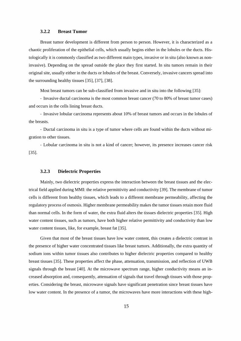
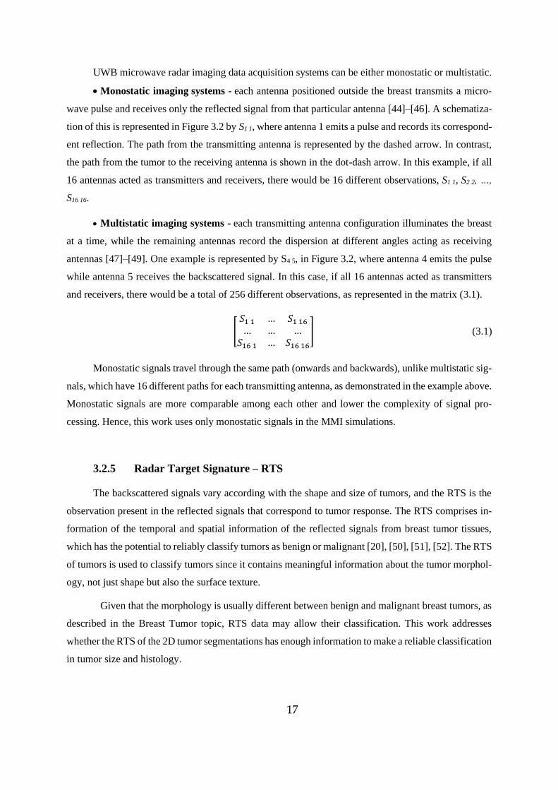
to the illumination of the breast with a microwave pulse emitted by one or more transmitting antennas.

The signals reflected by the tissues are then recorded by antennas, acting as receivers, as exemplified

in Figure 3.2. This schematic represents a breast model surrounded by 16 equally distanced antennas

and an object under test (i.e., tumor) in the center.

Figure 3.2 - Schematic of a 2D assembly of a UWB Microwave Radar Imaging, which emits UWB microwave

pulses from the transmitting antennas, represented as dashed arrows and collects the backscattered signals back to

the receiving antennas that come from the object under test, represented as dot-dashed arrows [35].

17

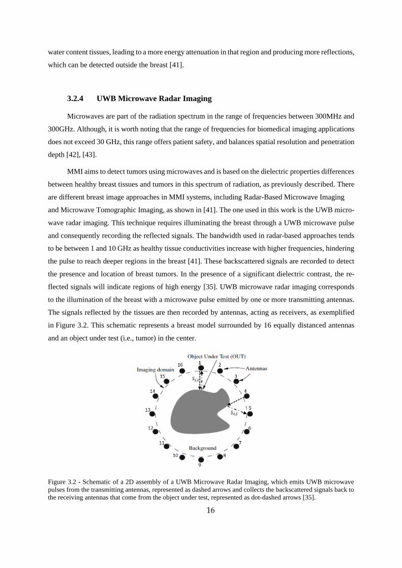
UWB microwave radar imaging data acquisition systems can be either monostatic or multistatic.

• Monostatic imaging systems - each antenna positioned outside the breast transmits a micro-

wave pulse and receives only the reflected signal from that particular antenna [44]–[46]. A schematiza-

tion of this is represented in Figure 3.2 by S1 1, where antenna 1 emits a pulse and records its correspond-

ent reflection. The path from the transmitting antenna is represented by the dashed arrow. In contrast,

the path from the tumor to the receiving antenna is shown in the dot-dash arrow. In this example, if all

16 antennas acted as transmitters and receivers, there would be 16 different observations, S1 1, S2 2, …,

S16 16.

• Multistatic imaging systems - each transmitting antenna configuration illuminates the breast

at a time, while the remaining antennas record the dispersion at different angles acting as receiving

antennas [47]–[49]. One example is represented by S4 5, in Figure 3.2, where antenna 4 emits the pulse

while antenna 5 receives the backscattered signal. In this case, if all 16 antennas acted as transmitters

and receivers, there would be a total of 256 different observations, as represented in the matrix (3.1).

[𝑆1 1 … 𝑆1 16

… … …𝑆16 1 … 𝑆16 16

] (3.1)

Monostatic signals travel through the same path (onwards and backwards), unlike multistatic sig-

nals, which have 16 different paths for each transmitting antenna, as demonstrated in the example above.

Monostatic signals are more comparable among each other and lower the complexity of signal pro-

cessing. Hence, this work uses only monostatic signals in the MMI simulations.

3.2.5 Radar Target Signature – RTS

The backscattered signals vary according with the shape and size of tumors, and the RTS is the

observation present in the reflected signals that correspond to tumor response. The RTS comprises in-

formation of the temporal and spatial information of the reflected signals from breast tumor tissues,

which has the potential to reliably classify tumors as benign or malignant [20], [50], [51], [52]. The RTS

of tumors is used to classify tumors since it contains meaningful information about the tumor morphol-

ogy, not just shape but also the surface texture.

Given that the morphology is usually different between benign and malignant breast tumors, as

described in the Breast Tumor topic, RTS data may allow their classification. This work addresses

whether the RTS of the 2D tumor segmentations has enough information to make a reliable classification

in tumor size and histology.

18

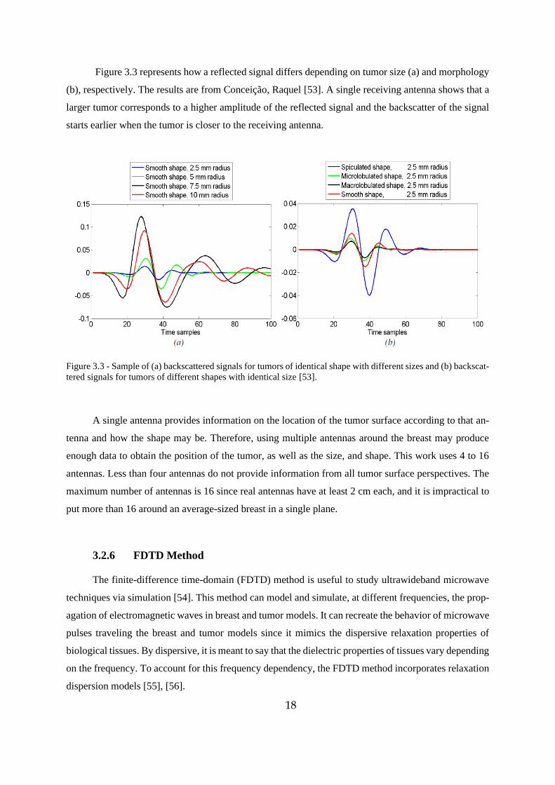
Figure 3.3 represents how a reflected signal differs depending on tumor size (a) and morphology

(b), respectively. The results are from Conceição, Raquel [53]. A single receiving antenna shows that a

larger tumor corresponds to a higher amplitude of the reflected signal and the backscatter of the signal

starts earlier when the tumor is closer to the receiving antenna.

Figure 3.3 - Sample of (a) backscattered signals for tumors of identical shape with different sizes and (b) backscat-

tered signals for tumors of different shapes with identical size [53].

A single antenna provides information on the location of the tumor surface according to that an-

tenna and how the shape may be. Therefore, using multiple antennas around the breast may produce

enough data to obtain the position of the tumor, as well as the size, and shape. This work uses 4 to 16

antennas. Less than four antennas do not provide information from all tumor surface perspectives. The

maximum number of antennas is 16 since real antennas have at least 2 cm each, and it is impractical to

put more than 16 around an average-sized breast in a single plane.

3.2.6 FDTD Method

The finite-difference time-domain (FDTD) method is useful to study ultrawideband microwave

techniques via simulation [54]. This method can model and simulate, at different frequencies, the prop-

agation of electromagnetic waves in breast and tumor models. It can recreate the behavior of microwave

pulses traveling the breast and tumor models since it mimics the dispersive relaxation properties of

biological tissues. By dispersive, it is meant to say that the dielectric properties of tissues vary depending

on the frequency. To account for this frequency dependency, the FDTD method incorporates relaxation

dispersion models [55], [56].

19

In this dissertation, the model used in the simulations to recreate the frequency-dependent propa-

gation characteristics of the tissues was the Debye model. This model has low computational complexity

but at the same time is reliable when recreating the dispersions due to dielectric properties contrast

between breast and tumor breast [54].

The Debye model is given by the following expression (3.2), that represents the permittivity as

an angular frequency function:

𝜀∗(𝜔) = 𝜀∞ + 𝜀𝑠 − 𝜀∞

1 + 𝑗𝜔𝜏+

𝜎𝑠

𝑗𝜔𝜀0 (3.2)

Where 𝜀0 is the vacuum permittivity, 𝜀∞ is the permittivity at the angular frequency 𝜔 = ∞ and

𝜀𝑠 is the permittivity at 𝜔 = 0, 𝜎𝑠 is the static ionic conductivity, 𝜏 represents the relaxation time con-

stant, and j is the imaginary number √−1 [57].

3.3 Materials

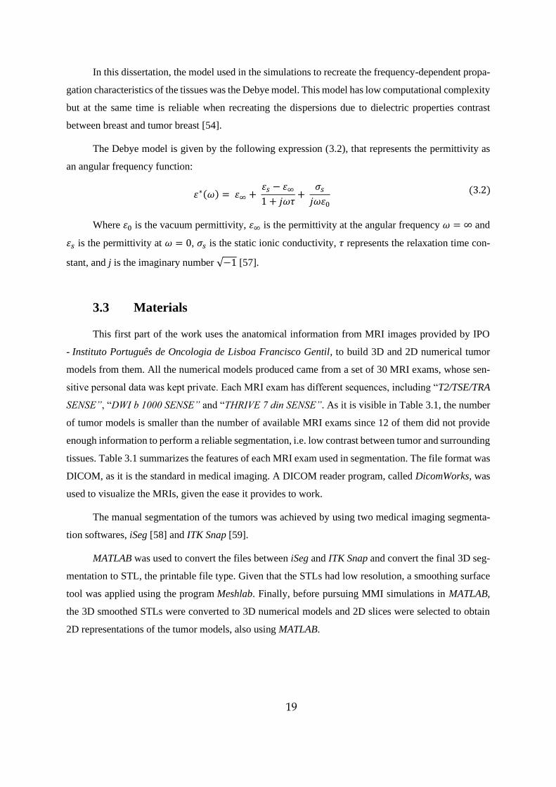
This first part of the work uses the anatomical information from MRI images provided by IPO

- Instituto Português de Oncologia de Lisboa Francisco Gentil, to build 3D and 2D numerical tumor

models from them. All the numerical models produced came from a set of 30 MRI exams, whose sen-

sitive personal data was kept private. Each MRI exam has different sequences, including “T2/TSE/TRA

SENSE”, “DWI b 1000 SENSE” and “THRIVE 7 din SENSE”. As it is visible in Table 3.1, the number

of tumor models is smaller than the number of available MRI exams since 12 of them did not provide

enough information to perform a reliable segmentation, i.e. low contrast between tumor and surrounding

tissues. Table 3.1 summarizes the features of each MRI exam used in segmentation. The file format was

DICOM, as it is the standard in medical imaging. A DICOM reader program, called DicomWorks, was

used to visualize the MRIs, given the ease it provides to work.

The manual segmentation of the tumors was achieved by using two medical imaging segmenta-

tion softwares, iSeg [58] and ITK Snap [59].

MATLAB was used to convert the files between iSeg and ITK Snap and convert the final 3D seg-

mentation to STL, the printable file type. Given that the STLs had low resolution, a smoothing surface

tool was applied using the program Meshlab. Finally, before pursuing MMI simulations in MATLAB,

the 3D smoothed STLs were converted to 3D numerical models and 2D slices were selected to obtain

2D representations of the tumor models, also using MATLAB.

20

Table 3.1 - MRI exams - dataset features.

MRI Histology Sex Age Plane Acquisition Resolution

(mm)

03 Invasive ductal carcinoma F 85 Axial 0.93 x 0.93 x 1


08 Invasive ductal carcinoma, intraduc-

tal component F 51 Axial 0.93 x 0.93 x 1



tal component, necrosis F 66 Axial 0.93 x 0.93 x 1

15 Mix Invasive carcinoma (lobular and

invasive) F 71 Axial 0.93 x 0.93 x 1



21 Invasive lobular carcinoma F 90 Axial 0.93 x 0.93 x 1




tal component, necrosis F 68 Axial 0.93 x 0.93 x 1

25 Ductal carcinoma in situ F 77 Axial 0.93 x 0.93 x 1

26 Invasive ductal carcinoma, ductal

carcinoma component in situ F 71 Axial 0.93 x 0.93 x 1

27 Papillary tumor with characteristics

of intraductal papilloma F 66 Axial 0.93 x 0.93 x 1

28 Invasive ductal carcinoma, scarce in-

traductal component, necrosis F 77 Axial 0.93 x 0.93 x 1

29 Ductal carcinoma in situ F 60 Axial 0.93 x 0.93 x 1

30 Fibroadenoma F 56 Axial 0.93 x 0.93 x 1

3.4 Methodology

This work consists of making numerical 3D and 2D tumors from segmenting MRI exams. After

that, the 2D numerical models produced are used in MMI simulations to recreate a UWB microwave

radar imaging system.

Step 1 of the methodology is to choose the sequence of images within each MRI exam that provide

better contrast between the tumors and the surrounding tissues.

Step 2 is about segmenting the tumors regions present in each image. The segmentation of an

image plays a crucial role in the extraction of information from it. The primary purpose of segmentation

is to allow the division of an image into several non-overlapping subregions. Specifically, it is a tech-

nique that allows isolating a region from the image under study. In medical imaging, the subregions of

an image correspond to different types of tissue, organs, or pathological structures, such as tumors [60].

21

This step involves using a semi-automatic clustering algorithm K-Means available in iSeg, which sepa-

rates each image into several clusters with identical pixel intensities. This algorithm facilitates the man-

ual segmentation in iSeg. ITK Snap software was used to manually correct tumor segmentations from

iSeg.

Step 3 shows how the 3D and 2D tumor numerical models are created in MATLAB and how it

was possible to smooth the tumor surfaces at different levels using Meshlab.

Finally, step 4 provides an overview of the MMI simulations performed using the 2D numerical

models from the segmentations.

Step 1 - Visualization and selection of MRI images using DicomWorks

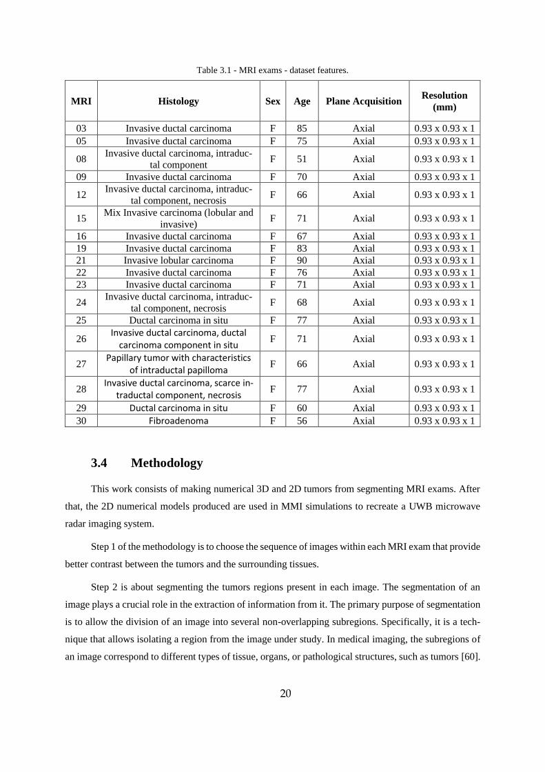
1.1 – DicomWorks is used to visualize all the different sequence of images in each MRI

exam. The sequence that provided the best contrast between tumors and the surrounding tissues was

“THRIVE 7 din SENSE”, which showed an axial view of the breasts, as shown in Figure 3.4. This

sequence is called “THRIVE 7 din SENSE” since it is dynamic and is recorded at seven different time

instances. The sequence presents individual 2D axial images (slices) of the patient that provide the 3D

anatomical representation of the tissues present when added together.

Figure 3.4 – Example of an axial plane MRI image using the THRIVE 7 din SENSE protocol from the repository

provided by IPO.

1.2 – After analyzing all seven different time samples from sequence “THRIVE 7 din SENSE”

for each patient, the one presenting the best contrast among all was selected. Moreover, the

slices that showed the tumor were saved as a new DICOM file, to be analyzed and segmented

using the iSeg software. To note that the file must be saved in the following format, Image{in-

dex}.dcm.

22

Step 2 - Tumor Segmentation

2.1- Segmentation using iSeg

The iSeg software was used to segment the visible tumors in each MRI, from the rest of the tissues,

given that pixels on tumor regions have different intensities compared to the surrounding pixels.

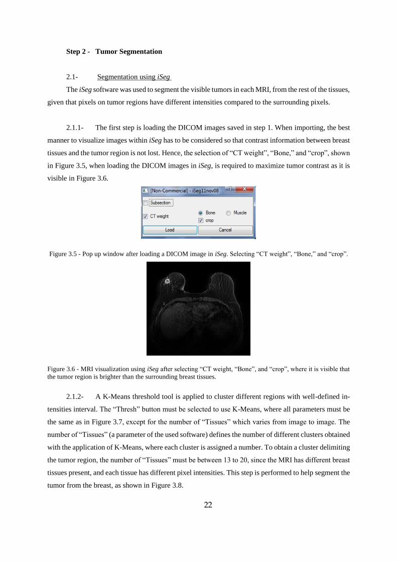
2.1.1- The first step is loading the DICOM images saved in step 1. When importing, the best

manner to visualize images within iSeg has to be considered so that contrast information between breast

tissues and the tumor region is not lost. Hence, the selection of “CT weight”, “Bone,” and “crop”, shown

in Figure 3.5, when loading the DICOM images in iSeg, is required to maximize tumor contrast as it is

visible in Figure 3.6.

Figure 3.5 - Pop up window after loading a DICOM image in iSeg. Selecting “CT weight”, “Bone,” and “crop”.

Figure 3.6 - MRI visualization using iSeg after selecting “CT weight, “Bone”, and “crop”, where it is visible that

the tumor region is brighter than the surrounding breast tissues.

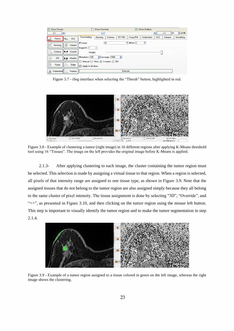
2.1.2- A K-Means threshold tool is applied to cluster different regions with well-defined in-

tensities interval. The “Thresh” button must be selected to use K-Means, where all parameters must be

the same as in Figure 3.7, except for the number of “Tissues” which varies from image to image. The

number of “Tissues” (a parameter of the used software) defines the number of different clusters obtained

with the application of K-Means, where each cluster is assigned a number. To obtain a cluster delimiting

the tumor region, the number of “Tissues” must be between 13 to 20, since the MRI has different breast

tissues present, and each tissue has different pixel intensities. This step is performed to help segment the

tumor from the breast, as shown in Figure 3.8.

23

Figure 3.7 - iSeg interface when selecting the “Thresh” button, highlighted in red.

Figure 3.8 - Example of clustering a tumor (right image) in 16 different regions after applying K-Means threshold

tool using 16 “Tissues”. The image on the left provides the original image before K-Means is applied.

2.1.3- After applying clustering to each image, the cluster containing the tumor region must

be selected. This selection is made by assigning a virtual tissue to that region. When a region is selected,

all pixels of that intensity range are assigned to one tissue type, as shown in Figure 3.9. Note that the

assigned tissues that do not belong to the tumor region are also assigned simply because they all belong

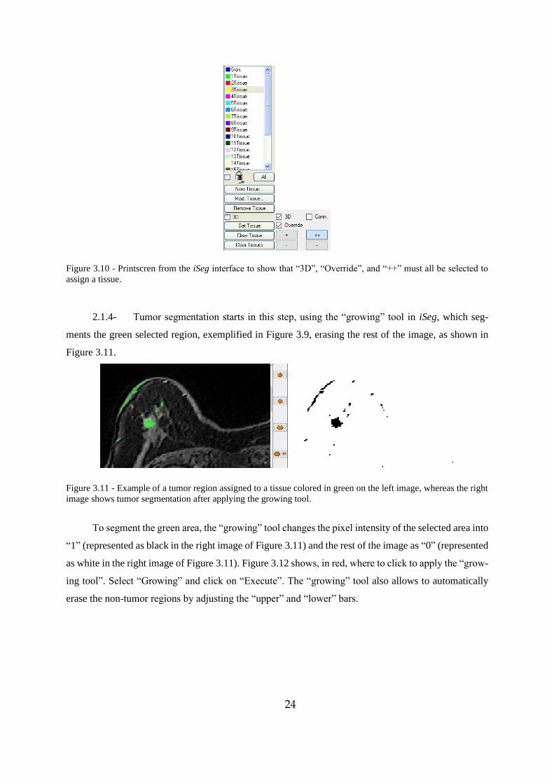
to the same cluster of pixel intensity. The tissue assignment is done by selecting "3D”, “Override”, and

“++”, as presented in Figure 3.10, and then clicking on the tumor region using the mouse left button.

This step is important to visually identify the tumor region and to make the tumor segmentation in step

2.1.4.

Figure 3.9 - Example of a tumor region assigned to a tissue colored in green on the left image, whereas the right

image shows the clustering.

24

Figure 3.10 - Printscren from the iSeg interface to show that “3D”, “Override”, and “++” must all be selected to

assign a tissue.

2.1.4- Tumor segmentation starts in this step, using the “growing” tool in iSeg, which seg-

ments the green selected region, exemplified in Figure 3.9, erasing the rest of the image, as shown in

Figure 3.11.


image shows tumor segmentation after applying the growing tool.

To segment the green area, the “growing” tool changes the pixel intensity of the selected area into

“1” (represented as black in the right image of Figure 3.11) and the rest of the image as “0” (represented

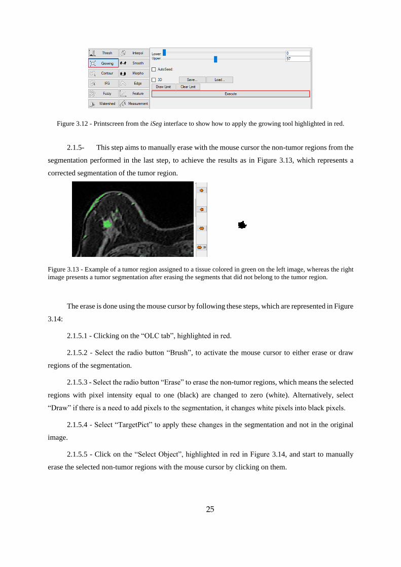
as white in the right image of Figure 3.11). Figure 3.12 shows, in red, where to click to apply the “grow-

ing tool”. Select “Growing” and click on “Execute”. The “growing” tool also allows to automatically

erase the non-tumor regions by adjusting the “upper” and “lower” bars.

25

Figure 3.12 - Printscreen from the iSeg interface to show how to apply the growing tool highlighted in red.

2.1.5- This step aims to manually erase with the mouse cursor the non-tumor regions from the

segmentation performed in the last step, to achieve the results as in Figure 3.13, which represents a

corrected segmentation of the tumor region.


image presents a tumor segmentation after erasing the segments that did not belong to the tumor region.

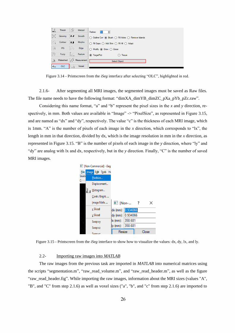
The erase is done using the mouse cursor by following these steps, which are represented in Figure

3.14:

2.1.5.1 - Clicking on the “OLC tab”, highlighted in red.

2.1.5.2 - Select the radio button “Brush”, to activate the mouse cursor to either erase or draw

regions of the segmentation.

2.1.5.3 - Select the radio button “Erase” to erase the non-tumor regions, which means the selected

regions with pixel intensity equal to one (black) are changed to zero (white). Alternatively, select

“Draw” if there is a need to add pixels to the segmentation, it changes white pixels into black pixels.

2.1.5.4 - Select “TargetPict” to apply these changes in the segmentation and not in the original

image.

2.1.5.5 - Click on the “Select Object”, highlighted in red in Figure 3.14, and start to manually

erase the selected non-tumor regions with the mouse cursor by clicking on them.

26

Figure 3.14 - Printscreen from the iSeg interface after selecting “OLC”, highlighted in red.

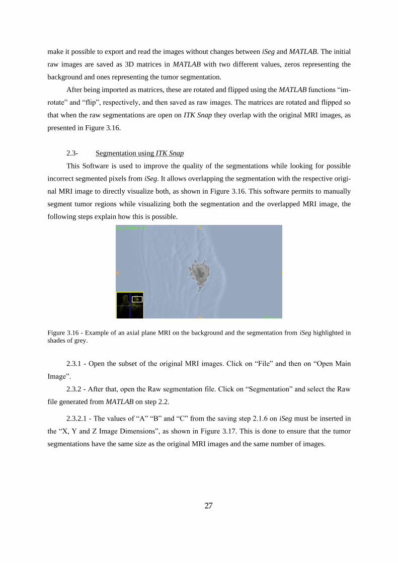
2.1.6- After segmenting all MRI images, the segmented images must be saved as Raw files.

The file name needs to have the following format: “dimXA_dimYB_dimZC_pXa_pYb_pZc.raw”.

Considering this name format, “a” and “b” represent the pixel sizes in the x and y direction, re-

spectively, in mm. Both values are available in “Image” -> “PixelSize”, as represented in Figure 3.15,

and are named as “dx” and “dy”, respectively. The value “c” is the thickness of each MRI image, which

is 1mm. “A” is the number of pixels of each image in the x direction, which corresponds to “lx”, the

length in mm in that direction, divided by dx, which is the image resolution in mm in the x direction, as

represented in Figure 3.15. “B” is the number of pixels of each image in the y direction, where “ly” and

“dy” are analog with lx and dx, respectively, but in the y direction. Finally, “C” is the number of saved

MRI images.

Figure 3.15 - Printscreen from the iSeg interface to show how to visualize the values: dx, dy, lx, and ly.

2.2- Importing raw images into MATLAB

The raw images from the previous task are imported in MATLAB into numerical matrices using

the scripts “segmentation.m”, “raw_read_volume.m”, and “raw_read_header.m”, as well as the figure

“raw_read_header.fig”. While importing the raw images, information about the MRI sizes (values "A",

"B", and "C" from step 2.1.6) as well as voxel sizes ("a", "b", and "c" from step 2.1.6) are imported to

27

make it possible to export and read the images without changes between iSeg and MATLAB. The initial

raw images are saved as 3D matrices in MATLAB with two different values, zeros representing the

background and ones representing the tumor segmentation.

After being imported as matrices, these are rotated and flipped using the MATLAB functions “im-

rotate” and “flip”, respectively, and then saved as raw images. The matrices are rotated and flipped so

that when the raw segmentations are open on ITK Snap they overlap with the original MRI images, as

presented in Figure 3.16.

2.3- Segmentation using ITK Snap

This Software is used to improve the quality of the segmentations while looking for possible

incorrect segmented pixels from iSeg. It allows overlapping the segmentation with the respective origi-

nal MRI image to directly visualize both, as shown in Figure 3.16. This software permits to manually

segment tumor regions while visualizing both the segmentation and the overlapped MRI image, the

following steps explain how this is possible.

Figure 3.16 - Example of an axial plane MRI on the background and the segmentation from iSeg highlighted in

shades of grey.

2.3.1 - Open the subset of the original MRI images. Click on “File” and then on “Open Main

Image”.

2.3.2 - After that, open the Raw segmentation file. Click on “Segmentation” and select the Raw

file generated from MATLAB on step 2.2.

2.3.2.1 - The values of “A” “B” and “C” from the saving step 2.1.6 on iSeg must be inserted in

the “X, Y and Z Image Dimensions”, as shown in Figure 3.17. This is done to ensure that the tumor

segmentations have the same size as the original MRI images and the same number of images.

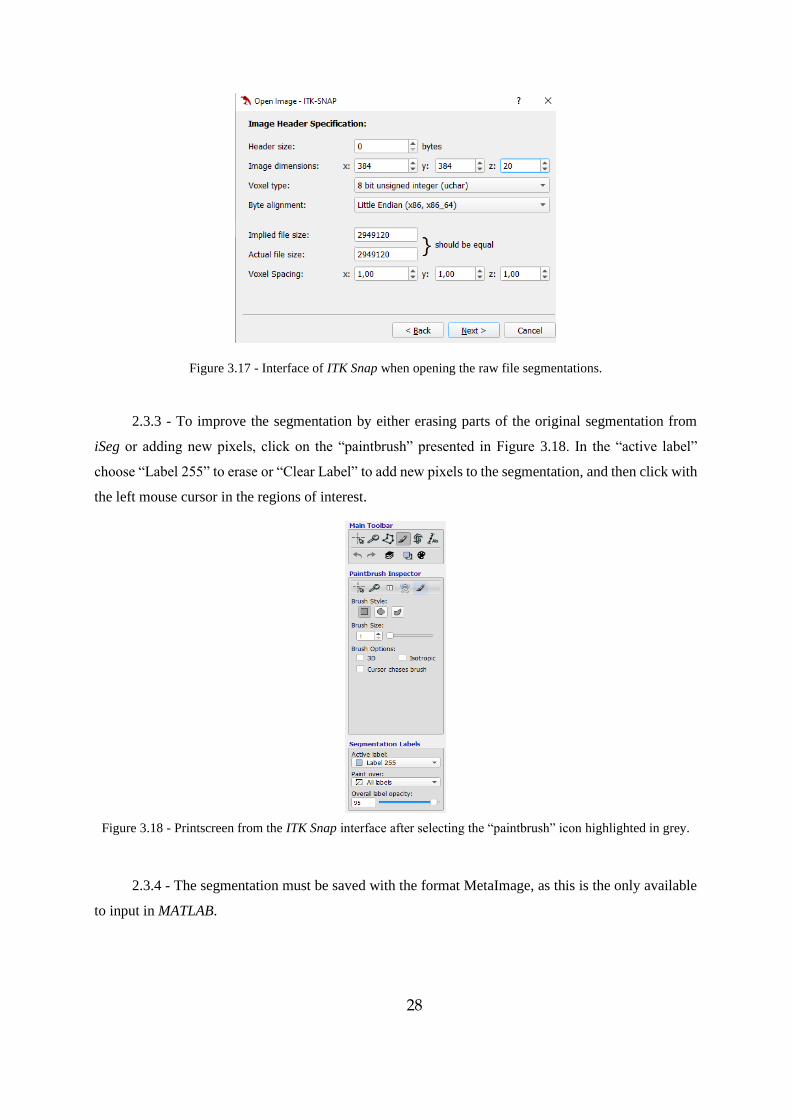
28

Figure 3.17 - Interface of ITK Snap when opening the raw file segmentations.

2.3.3 - To improve the segmentation by either erasing parts of the original segmentation from

iSeg or adding new pixels, click on the “paintbrush” presented in Figure 3.18. In the “active label”

choose “Label 255” to erase or “Clear Label” to add new pixels to the segmentation, and then click with

the left mouse cursor in the regions of interest.

Figure 3.18 - Printscreen from the ITK Snap interface after selecting the “paintbrush” icon highlighted in grey.

2.3.4 - The segmentation must be saved with the format MetaImage, as this is the only available

to input in MATLAB.

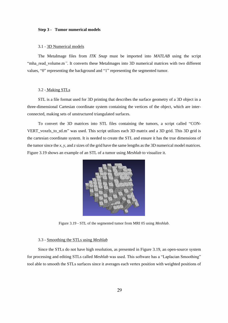
29

Step 3 - Tumor numerical models

3.1 - 3D Numerical models

The MetaImage files from ITK Snap must be imported into MATLAB using the script

“mha_read_volume.m”. It converts these MetaImages into 3D numerical matrices with two different

values, “0” representing the background and “1” representing the segmented tumor.

3.2 - Making STLs

STL is a file format used for 3D printing that describes the surface geometry of a 3D object in a

three-dimensional Cartesian coordinate system containing the vertices of the object, which are inter-

connected, making sets of unstructured triangulated surfaces.

To convert the 3D matrices into STL files containing the tumors, a script called “CON-

VERT_voxels_to_stl.m” was used. This script utilizes each 3D matrix and a 3D grid. This 3D grid is

the cartesian coordinate system. It is needed to create the STL and ensure it has the true dimensions of

the tumor since the x, y, and z sizes of the grid have the same lengths as the 3D numerical model matrices.

Figure 3.19 shows an example of an STL of a tumor using Meshlab to visualize it.

Figure 3.19 - STL of the segmented tumor from MRI 05 using Meshlab.

3.3 - Smoothing the STLs using Meshlab

Since the STLs do not have high resolution, as presented in Figure 3.19, an open-source system

for processing and editing STLs called Meshlab was used. This software has a “Laplacian Smoothing”

tool able to smooth the STLs surfaces since it averages each vertex position with weighted positions of

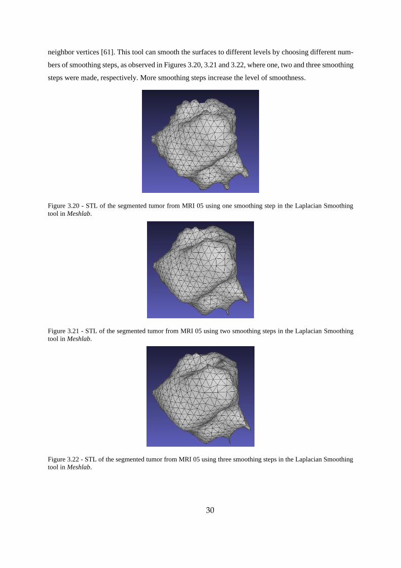
30

neighbor vertices [61]. This tool can smooth the surfaces to different levels by choosing different num-

bers of smoothing steps, as observed in Figures 3.20, 3.21 and 3.22, where one, two and three smoothing

steps were made, respectively. More smoothing steps increase the level of smoothness.

Figure 3.20 - STL of the segmented tumor from MRI 05 using one smoothing step in the Laplacian Smoothing

tool in Meshlab.

Figure 3.21 - STL of the segmented tumor from MRI 05 using two smoothing steps in the Laplacian Smoothing

tool in Meshlab.

Figure 3.22 - STL of the segmented tumor from MRI 05 using three smoothing steps in the Laplacian Smoothing

tool in Meshlab.

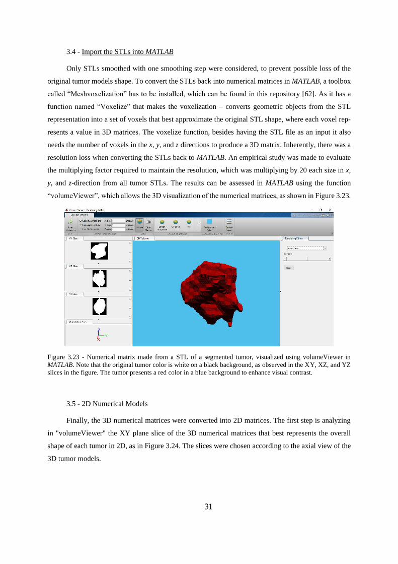
31

3.4 - Import the STLs into MATLAB

Only STLs smoothed with one smoothing step were considered, to prevent possible loss of the

original tumor models shape. To convert the STLs back into numerical matrices in MATLAB, a toolbox

called “Meshvoxelization” has to be installed, which can be found in this repository [62]. As it has a

function named “Voxelize” that makes the voxelization – converts geometric objects from the STL

representation into a set of voxels that best approximate the original STL shape, where each voxel rep-

resents a value in 3D matrices. The voxelize function, besides having the STL file as an input it also

needs the number of voxels in the x, y, and z directions to produce a 3D matrix. Inherently, there was a

resolution loss when converting the STLs back to MATLAB. An empirical study was made to evaluate

the multiplying factor required to maintain the resolution, which was multiplying by 20 each size in x,

y, and z-direction from all tumor STLs. The results can be assessed in MATLAB using the function

“volumeViewer”, which allows the 3D visualization of the numerical matrices, as shown in Figure 3.23.

Figure 3.23 - Numerical matrix made from a STL of a segmented tumor, visualized using volumeViewer in

MATLAB. Note that the original tumor color is white on a black background, as observed in the XY, XZ, and YZ

slices in the figure. The tumor presents a red color in a blue background to enhance visual contrast.

3.5 - 2D Numerical Models

Finally, the 3D numerical matrices were converted into 2D matrices. The first step is analyzing

in "volumeViewer" the XY plane slice of the 3D numerical matrices that best represents the overall

shape of each tumor in 2D, as in Figure 3.24. The slices were chosen according to the axial view of the

3D tumor models.

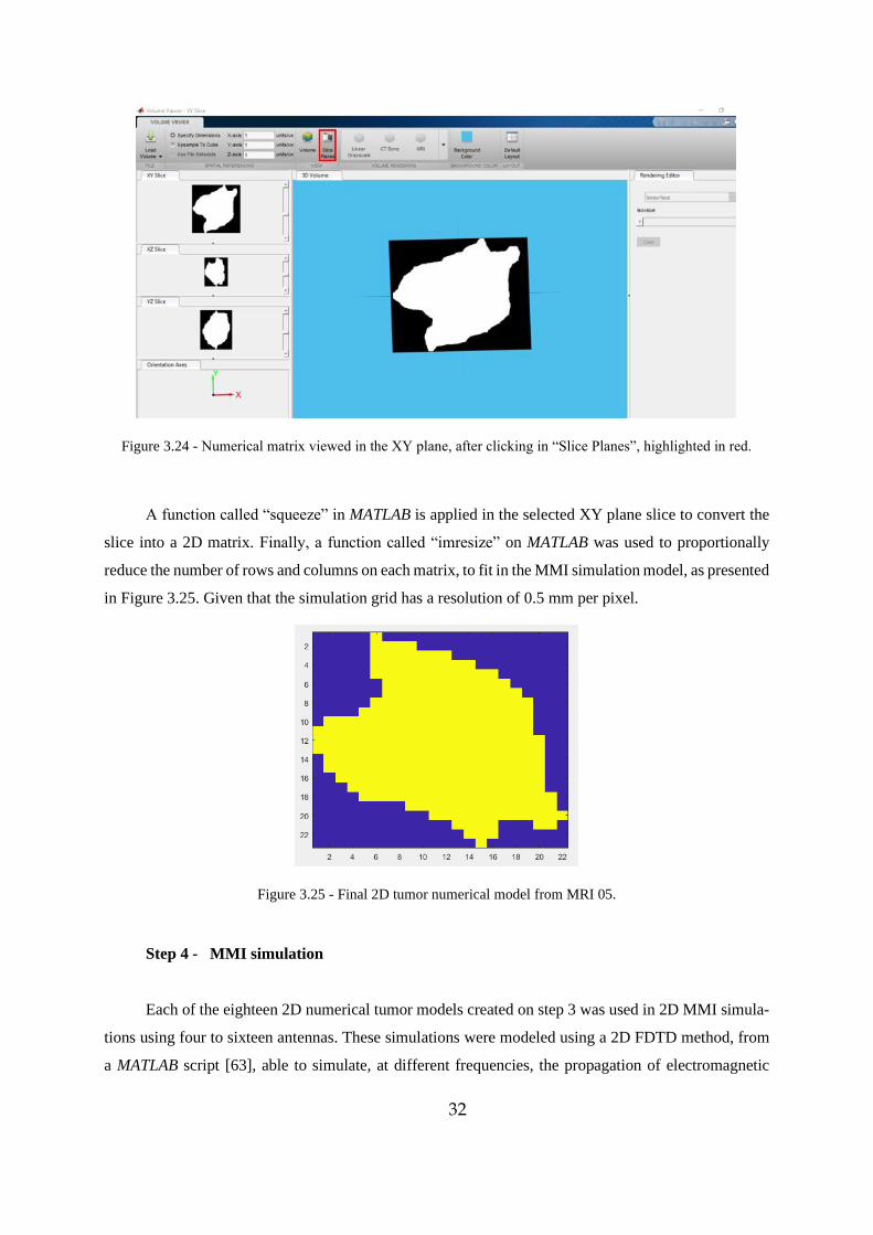
32

Figure 3.24 - Numerical matrix viewed in the XY plane, after clicking in “Slice Planes”, highlighted in red.

A function called “squeeze” in MATLAB is applied in the selected XY plane slice to convert the

slice into a 2D matrix. Finally, a function called “imresize” on MATLAB was used to proportionally

reduce the number of rows and columns on each matrix, to fit in the MMI simulation model, as presented

in Figure 3.25. Given that the simulation grid has a resolution of 0.5 mm per pixel.

Figure 3.25 - Final 2D tumor numerical model from MRI 05.

Step 4 - MMI simulation

Each of the eighteen 2D numerical tumor models created on step 3 was used in 2D MMI simula-

tions using four to sixteen antennas. These simulations were modeled using a 2D FDTD method, from

a MATLAB script [63], able to simulate, at different frequencies, the propagation of electromagnetic

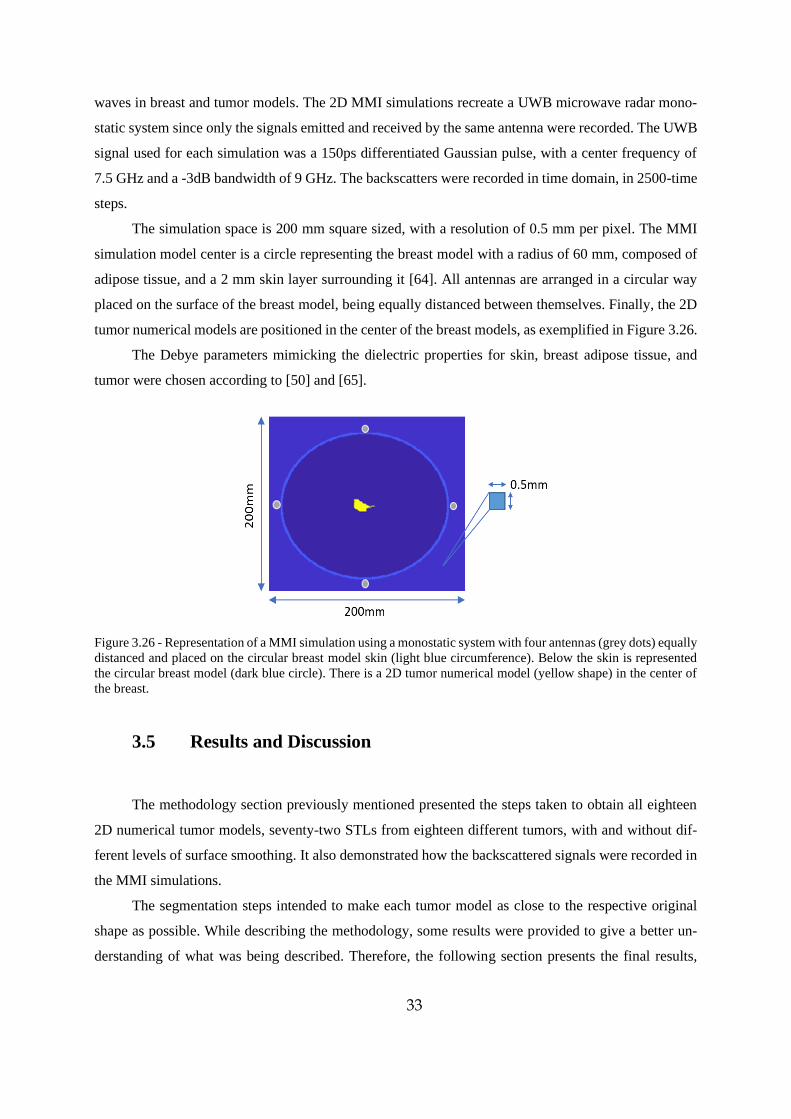
33

waves in breast and tumor models. The 2D MMI simulations recreate a UWB microwave radar mono-

static system since only the signals emitted and received by the same antenna were recorded. The UWB

signal used for each simulation was a 150ps differentiated Gaussian pulse, with a center frequency of

7.5 GHz and a -3dB bandwidth of 9 GHz. The backscatters were recorded in time domain, in 2500-time

steps.

The simulation space is 200 mm square sized, with a resolution of 0.5 mm per pixel. The MMI

simulation model center is a circle representing the breast model with a radius of 60 mm, composed of

adipose tissue, and a 2 mm skin layer surrounding it [64]. All antennas are arranged in a circular way

placed on the surface of the breast model, being equally distanced between themselves. Finally, the 2D

tumor numerical models are positioned in the center of the breast models, as exemplified in Figure 3.26.

The Debye parameters mimicking the dielectric properties for skin, breast adipose tissue, and

tumor were chosen according to [50] and [65].

Figure 3.26 - Representation of a MMI simulation using a monostatic system with four antennas (grey dots) equally

distanced and placed on the circular breast model skin (light blue circumference). Below the skin is represented

the circular breast model (dark blue circle). There is a 2D tumor numerical model (yellow shape) in the center of

the breast.

3.5 Results and Discussion

The methodology section previously mentioned presented the steps taken to obtain all eighteen

2D numerical tumor models, seventy-two STLs from eighteen different tumors, with and without dif-

ferent levels of surface smoothing. It also demonstrated how the backscattered signals were recorded in

the MMI simulations.

The segmentation steps intended to make each tumor model as close to the respective original

shape as possible. While describing the methodology, some results were provided to give a better un-

derstanding of what was being described. Therefore, the following section presents the final results,

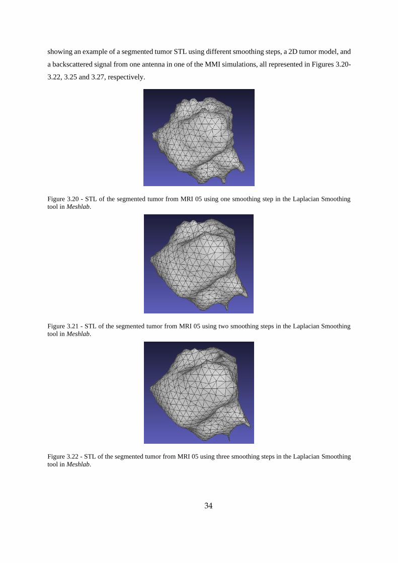
34

showing an example of a segmented tumor STL using different smoothing steps, a 2D tumor model, and

a backscattered signal from one antenna in one of the MMI simulations, all represented in Figures 3.20-

3.22, 3.25 and 3.27, respectively.

Figure 3.20 - STL of the segmented tumor from MRI 05 using one smoothing step in the Laplacian Smoothing

tool in Meshlab.

Figure 3.21 - STL of the segmented tumor from MRI 05 using two smoothing steps in the Laplacian Smoothing

tool in Meshlab.

Figure 3.22 - STL of the segmented tumor from MRI 05 using three smoothing steps in the Laplacian Smoothing

tool in Meshlab.

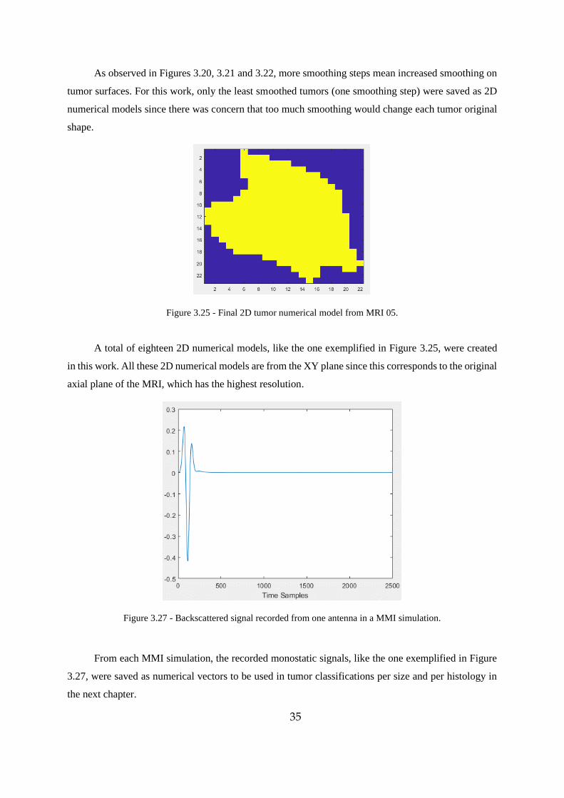
35

As observed in Figures 3.20, 3.21 and 3.22, more smoothing steps mean increased smoothing on

tumor surfaces. For this work, only the least smoothed tumors (one smoothing step) were saved as 2D

numerical models since there was concern that too much smoothing would change each tumor original

shape.

Figure 3.25 - Final 2D tumor numerical model from MRI 05.

A total of eighteen 2D numerical models, like the one exemplified in Figure 3.25, were created

in this work. All these 2D numerical models are from the XY plane since this corresponds to the original

axial plane of the MRI, which has the highest resolution.

Figure 3.27 - Backscattered signal recorded from one antenna in a MMI simulation.

From each MMI simulation, the recorded monostatic signals, like the one exemplified in Figure

3.27, were saved as numerical vectors to be used in tumor classifications per size and per histology in

the next chapter.

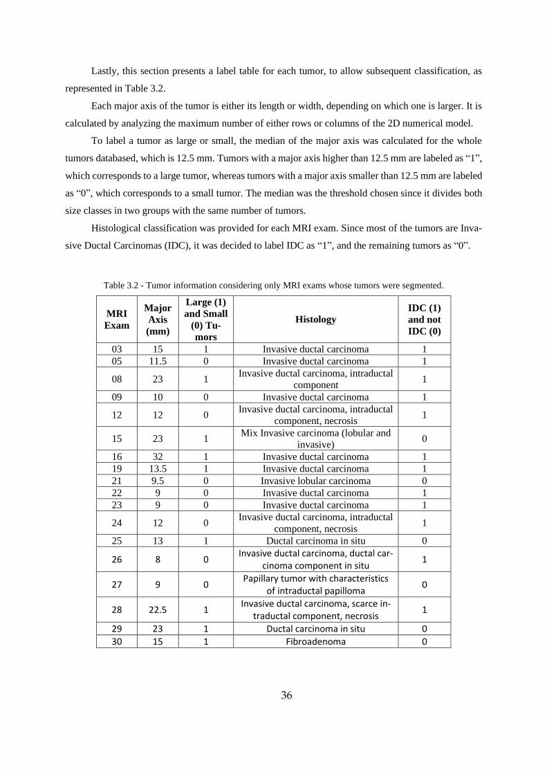
36

Lastly, this section presents a label table for each tumor, to allow subsequent classification, as

represented in Table 3.2.

Each major axis of the tumor is either its length or width, depending on which one is larger. It is

calculated by analyzing the maximum number of either rows or columns of the 2D numerical model.

To label a tumor as large or small, the median of the major axis was calculated for the whole

tumors databased, which is 12.5 mm. Tumors with a major axis higher than 12.5 mm are labeled as “1”,

which corresponds to a large tumor, whereas tumors with a major axis smaller than 12.5 mm are labeled

as “0”, which corresponds to a small tumor. The median was the threshold chosen since it divides both

size classes in two groups with the same number of tumors.

Histological classification was provided for each MRI exam. Since most of the tumors are Inva-

sive Ductal Carcinomas (IDC), it was decided to label IDC as “1”, and the remaining tumors as “0”.

Table 3.2 - Tumor information considering only MRI exams whose tumors were segmented.

MRI

Exam

Major

Axis

(mm)

Large (1)

and Small

(0) Tu-

mors

Histology

IDC (1)

and not

IDC (0)

03 15 1 Invasive ductal carcinoma 1

05 11.5 0 Invasive ductal carcinoma 1

08 23 1 Invasive ductal carcinoma, intraductal

component 1



component, necrosis 1

15 23 1 Mix Invasive carcinoma (lobular and

invasive) 0


19 13.5 1 Invasive ductal carcinoma 1

21 9.5 0 Invasive lobular carcinoma 0




component, necrosis 1

25 13 1 Ductal carcinoma in situ 0

26 8 0 Invasive ductal carcinoma, ductal car-

cinoma component in situ 1

27 9 0 Papillary tumor with characteristics

of intraductal papilloma 0

28 22.5 1 Invasive ductal carcinoma, scarce in-

traductal component, necrosis 1

29 23 1 Ductal carcinoma in situ 0

30 15 1 Fibroadenoma 0

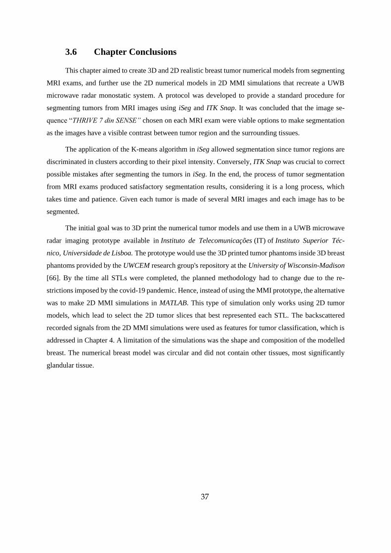
37

3.6 Chapter Conclusions

This chapter aimed to create 3D and 2D realistic breast tumor numerical models from segmenting

MRI exams, and further use the 2D numerical models in 2D MMI simulations that recreate a UWB

microwave radar monostatic system. A protocol was developed to provide a standard procedure for

segmenting tumors from MRI images using iSeg and ITK Snap. It was concluded that the image se-

quence “THRIVE 7 din SENSE” chosen on each MRI exam were viable options to make segmentation

as the images have a visible contrast between tumor region and the surrounding tissues.

The application of the K-means algorithm in iSeg allowed segmentation since tumor regions are

discriminated in clusters according to their pixel intensity. Conversely, ITK Snap was crucial to correct

possible mistakes after segmenting the tumors in iSeg. In the end, the process of tumor segmentation

from MRI exams produced satisfactory segmentation results, considering it is a long process, which

takes time and patience. Given each tumor is made of several MRI images and each image has to be

segmented.

The initial goal was to 3D print the numerical tumor models and use them in a UWB microwave

radar imaging prototype available in Instituto de Telecomunicações (IT) of Instituto Superior Téc-

nico, Universidade de Lisboa. The prototype would use the 3D printed tumor phantoms inside 3D breast

phantoms provided by the UWCEM research group's repository at the University of Wisconsin-Madison

[66]. By the time all STLs were completed, the planned methodology had to change due to the re-

strictions imposed by the covid-19 pandemic. Hence, instead of using the MMI prototype, the alternative

was to make 2D MMI simulations in MATLAB. This type of simulation only works using 2D tumor

models, which lead to select the 2D tumor slices that best represented each STL. The backscattered

recorded signals from the 2D MMI simulations were used as features for tumor classification, which is

addressed in Chapter 4. A limitation of the simulations was the shape and composition of the modelled

breast. The numerical breast model was circular and did not contain other tissues, most significantly

glandular tissue.

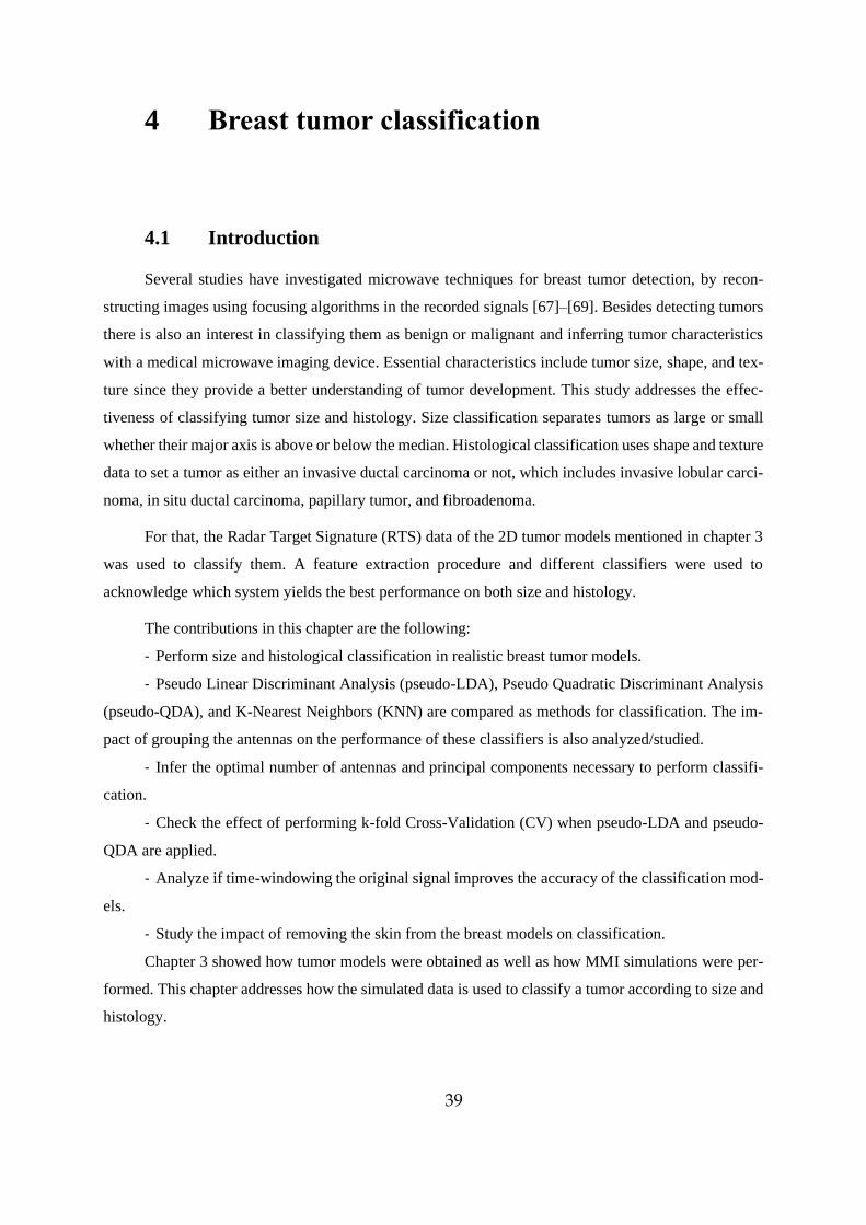
39

4 Breast tumor classification

4.1 Introduction

Several studies have investigated microwave techniques for breast tumor detection, by recon-

structing images using focusing algorithms in the recorded signals [67]–[69]. Besides detecting tumors

there is also an interest in classifying them as benign or malignant and inferring tumor characteristics

with a medical microwave imaging device. Essential characteristics include tumor size, shape, and tex-

ture since they provide a better understanding of tumor development. This study addresses the effec-

tiveness of classifying tumor size and histology. Size classification separates tumors as large or small

whether their major axis is above or below the median. Histological classification uses shape and texture

data to set a tumor as either an invasive ductal carcinoma or not, which includes invasive lobular carci-

noma, in situ ductal carcinoma, papillary tumor, and fibroadenoma.

For that, the Radar Target Signature (RTS) data of the 2D tumor models mentioned in chapter 3

was used to classify them. A feature extraction procedure and different classifiers were used to

acknowledge which system yields the best performance on both size and histology.

The contributions in this chapter are the following:

- Perform size and histological classification in realistic breast tumor models.

- Pseudo Linear Discriminant Analysis (pseudo-LDA), Pseudo Quadratic Discriminant Analysis

(pseudo-QDA), and K-Nearest Neighbors (KNN) are compared as methods for classification. The im-

pact of grouping the antennas on the performance of these classifiers is also analyzed/studied.

- Infer the optimal number of antennas and principal components necessary to perform classifi-

cation.

- Check the effect of performing k-fold Cross-Validation (CV) when pseudo-LDA and pseudo-

QDA are applied.

- Analyze if time-windowing the original signal improves the accuracy of the classification mod-

els.

- Study the impact of removing the skin from the breast models on classification.

Chapter 3 showed how tumor models were obtained as well as how MMI simulations were per-

formed. This chapter addresses how the simulated data is used to classify a tumor according to size and

histology.

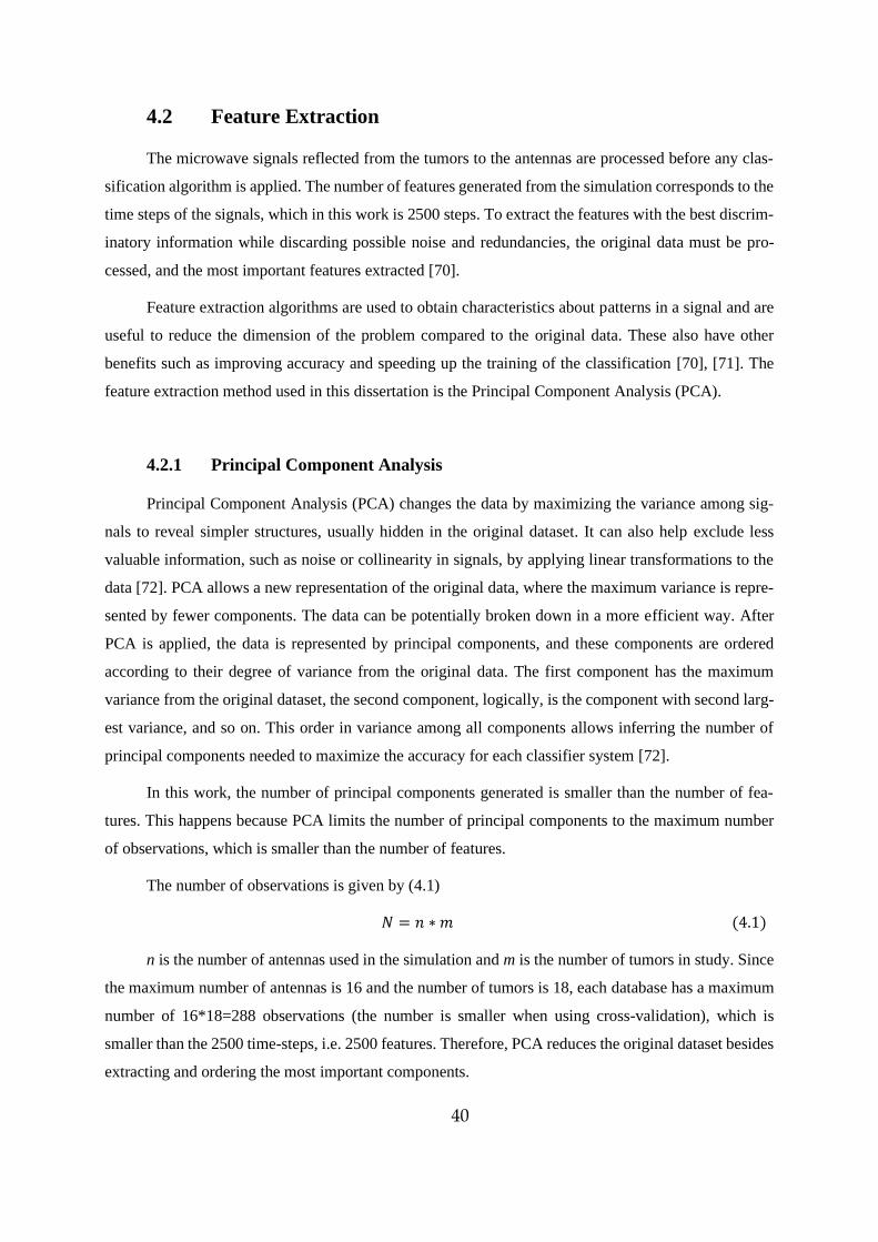
40

4.2 Feature Extraction

The microwave signals reflected from the tumors to the antennas are processed before any clas-

sification algorithm is applied. The number of features generated from the simulation corresponds to the

time steps of the signals, which in this work is 2500 steps. To extract the features with the best discrim-

inatory information while discarding possible noise and redundancies, the original data must be pro-

cessed, and the most important features extracted [70].

Feature extraction algorithms are used to obtain characteristics about patterns in a signal and are

useful to reduce the dimension of the problem compared to the original data. These also have other

benefits such as improving accuracy and speeding up the training of the classification [70], [71]. The

feature extraction method used in this dissertation is the Principal Component Analysis (PCA).

4.2.1 Principal Component Analysis

Principal Component Analysis (PCA) changes the data by maximizing the variance among sig-

nals to reveal simpler structures, usually hidden in the original dataset. It can also help exclude less

valuable information, such as noise or collinearity in signals, by applying linear transformations to the

data [72]. PCA allows a new representation of the original data, where the maximum variance is repre-

sented by fewer components. The data can be potentially broken down in a more efficient way. After

PCA is applied, the data is represented by principal components, and these components are ordered

according to their degree of variance from the original data. The first component has the maximum

variance from the original dataset, the second component, logically, is the component with second larg-

est variance, and so on. This order in variance among all components allows inferring the number of

principal components needed to maximize the accuracy for each classifier system [72].

In this work, the number of principal components generated is smaller than the number of fea-

tures. This happens because PCA limits the number of principal components to the maximum number

of observations, which is smaller than the number of features.

The number of observations is given by (4.1)

𝑁 = 𝑛 ∗ 𝑚 (4.1)

n is the number of antennas used in the simulation and m is the number of tumors in study. Since

the maximum number of antennas is 16 and the number of tumors is 18, each database has a maximum

number of 16*18=288 observations (the number is smaller when using cross-validation), which is

smaller than the 2500 time-steps, i.e. 2500 features. Therefore, PCA reduces the original dataset besides

extracting and ordering the most important components.

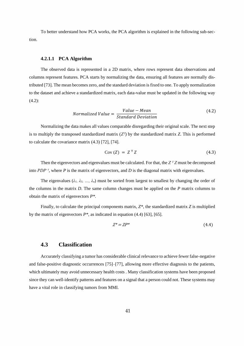
41

To better understand how PCA works, the PCA algorithm is explained in the following sub-sec-

tion.

4.2.1.1 PCA Algorithm

The observed data is represented in a 2D matrix, where rows represent data observations and

columns represent features. PCA starts by normalizing the data, ensuring all features are normally dis-

tributed [73]. The mean becomes zero, and the standard deviation is fixed to one. To apply normalization

to the dataset and achieve a standardized matrix, each data-value must be updated in the following way

(4.2):

𝑁𝑜𝑟𝑚𝑎𝑙𝑖𝑧𝑒𝑑 𝑉𝑎𝑙𝑢𝑒 =

𝑉𝑎𝑙𝑢𝑒 − 𝑀𝑒𝑎𝑛

𝑆𝑡𝑎𝑛𝑑𝑎𝑟𝑑 𝐷𝑒𝑣𝑖𝑎𝑡𝑖𝑜𝑛

(4.2)

Normalizing the data makes all values comparable disregarding their original scale. The next step

is to multiply the transposed standardized matrix (Zᵀ) by the standardized matrix Z. This is performed

to calculate the covariance matrix (4.3) [72], [74].

Cov (𝑍) = 𝑍 ᵀ 𝑍 (4.3)

Then the eigenvectors and eigenvalues must be calculated. For that, the Z T Z must be decomposed

into PDP⁻¹, where P is the matrix of eigenvectors, and D is the diagonal matrix with eigenvalues.

The eigenvalues (λ₁, λ₂, …, λn) must be sorted from largest to smallest by changing the order of

the columns in the matrix D. The same column changes must be applied on the P matrix columns to

obtain the matrix of eigenvectors P*.

Finally, to calculate the principal components matrix, Z*, the standardized matrix Z is multiplied

by the matrix of eigenvectors P*, as indicated in equation (4.4) [63], [65].

Z* = ZP* (4.4)

4.3 Classification

Accurately classifying a tumor has considerable clinical relevance to achieve fewer false-negative

and false-positive diagnostic occurrences [75]–[77], allowing more effective diagnosis to the patients,

which ultimately may avoid unnecessary health costs . Many classification systems have been proposed

since they can well-identify patterns and features on a signal that a person could not. These systems may

have a vital role in classifying tumors from MMI.

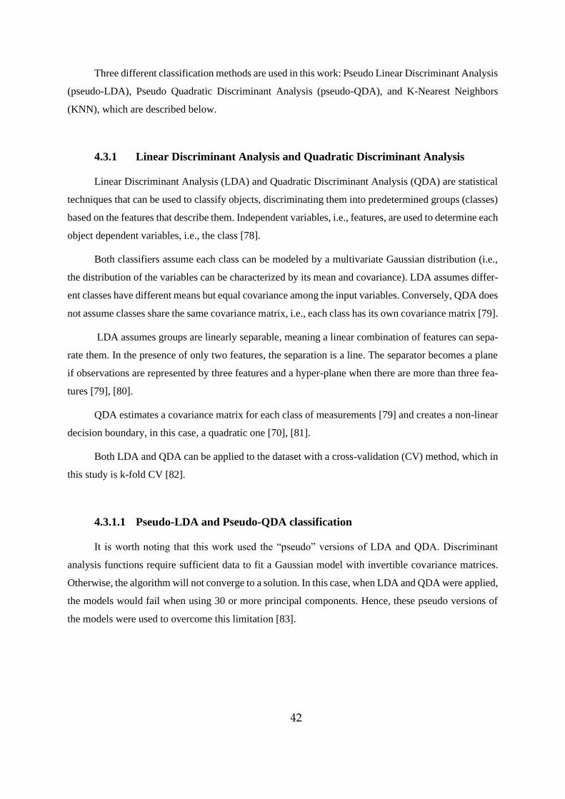
42

Three different classification methods are used in this work: Pseudo Linear Discriminant Analysis

(pseudo-LDA), Pseudo Quadratic Discriminant Analysis (pseudo-QDA), and K-Nearest Neighbors

(KNN), which are described below.

4.3.1 Linear Discriminant Analysis and Quadratic Discriminant Analysis

Linear Discriminant Analysis (LDA) and Quadratic Discriminant Analysis (QDA) are statistical

techniques that can be used to classify objects, discriminating them into predetermined groups (classes)

based on the features that describe them. Independent variables, i.e., features, are used to determine each

object dependent variables, i.e., the class [78].

Both classifiers assume each class can be modeled by a multivariate Gaussian distribution (i.e.,

the distribution of the variables can be characterized by its mean and covariance). LDA assumes differ-

ent classes have different means but equal covariance among the input variables. Conversely, QDA does

not assume classes share the same covariance matrix, i.e., each class has its own covariance matrix [79].

LDA assumes groups are linearly separable, meaning a linear combination of features can sepa-

rate them. In the presence of only two features, the separation is a line. The separator becomes a plane

if observations are represented by three features and a hyper-plane when there are more than three fea-

tures [79], [80].

QDA estimates a covariance matrix for each class of measurements [79] and creates a non-linear

decision boundary, in this case, a quadratic one [70], [81].

Both LDA and QDA can be applied to the dataset with a cross-validation (CV) method, which in

this study is k-fold CV [82].

4.3.1.1 Pseudo-LDA and Pseudo-QDA classification

It is worth noting that this work used the “pseudo” versions of LDA and QDA. Discriminant

analysis functions require sufficient data to fit a Gaussian model with invertible covariance matrices.

Otherwise, the algorithm will not converge to a solution. In this case, when LDA and QDA were applied,

the models would fail when using 30 or more principal components. Hence, these pseudo versions of

the models were used to overcome this limitation [83].

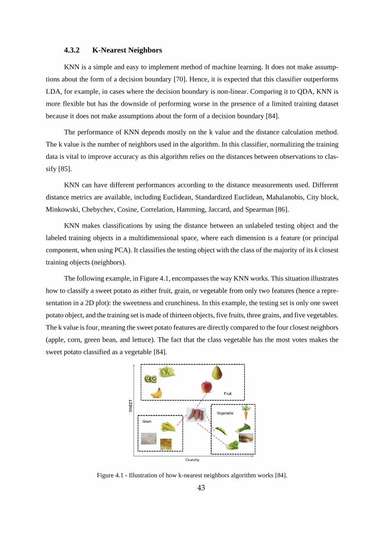
43

4.3.2 K-Nearest Neighbors

KNN is a simple and easy to implement method of machine learning. It does not make assump-

tions about the form of a decision boundary [70]. Hence, it is expected that this classifier outperforms

LDA, for example, in cases where the decision boundary is non-linear. Comparing it to QDA, KNN is

more flexible but has the downside of performing worse in the presence of a limited training dataset

because it does not make assumptions about the form of a decision boundary [84].

The performance of KNN depends mostly on the k value and the distance calculation method.

The k value is the number of neighbors used in the algorithm. In this classifier, normalizing the training

data is vital to improve accuracy as this algorithm relies on the distances between observations to clas-

sify [85].

KNN can have different performances according to the distance measurements used. Different

distance metrics are available, including Euclidean, Standardized Euclidean, Mahalanobis, City block,

Minkowski, Chebychev, Cosine, Correlation, Hamming, Jaccard, and Spearman [86].

KNN makes classifications by using the distance between an unlabeled testing object and the

labeled training objects in a multidimensional space, where each dimension is a feature (or principal

component, when using PCA). It classifies the testing object with the class of the majority of its k closest

training objects (neighbors).

The following example, in Figure 4.1, encompasses the way KNN works. This situation illustrates

how to classify a sweet potato as either fruit, grain, or vegetable from only two features (hence a repre-

sentation in a 2D plot): the sweetness and crunchiness. In this example, the testing set is only one sweet

potato object, and the training set is made of thirteen objects, five fruits, three grains, and five vegetables.

The k value is four, meaning the sweet potato features are directly compared to the four closest neighbors

(apple, corn, green bean, and lettuce). The fact that the class vegetable has the most votes makes the

sweet potato classified as a vegetable [84].

Figure 4.1 - Illustration of how k-nearest neighbors algorithm works [84].

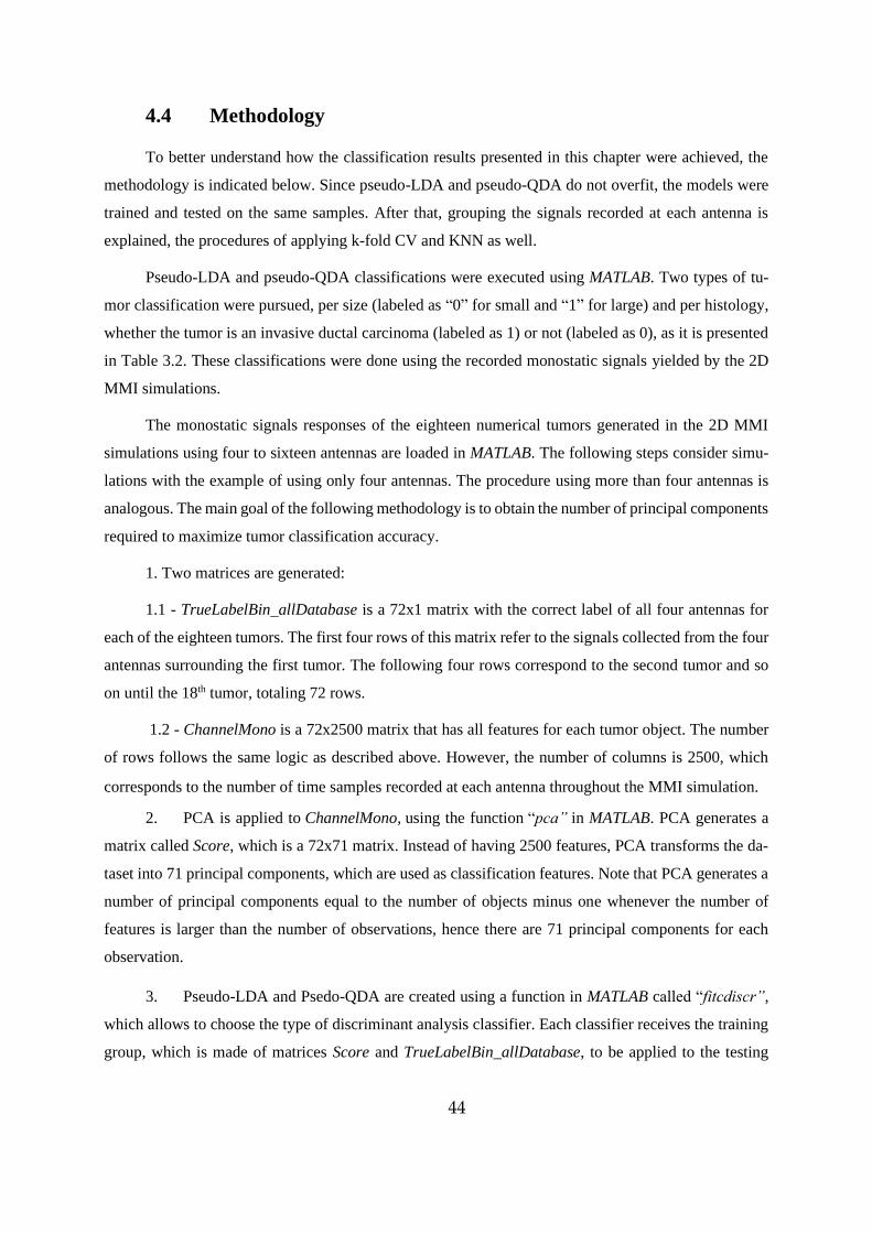
44

4.4 Methodology

To better understand how the classification results presented in this chapter were achieved, the

methodology is indicated below. Since pseudo-LDA and pseudo-QDA do not overfit, the models were

trained and tested on the same samples. After that, grouping the signals recorded at each antenna is

explained, the procedures of applying k-fold CV and KNN as well.

Pseudo-LDA and pseudo-QDA classifications were executed using MATLAB. Two types of tu-

mor classification were pursued, per size (labeled as “0” for small and “1” for large) and per histology,

whether the tumor is an invasive ductal carcinoma (labeled as 1) or not (labeled as 0), as it is presented

in Table 3.2. These classifications were done using the recorded monostatic signals yielded by the 2D

MMI simulations.

The monostatic signals responses of the eighteen numerical tumors generated in the 2D MMI

simulations using four to sixteen antennas are loaded in MATLAB. The following steps consider simu-

lations with the example of using only four antennas. The procedure using more than four antennas is

analogous. The main goal of the following methodology is to obtain the number of principal components

required to maximize tumor classification accuracy.

1. Two matrices are generated:

1.1 - TrueLabelBin_allDatabase is a 72x1 matrix with the correct label of all four antennas for

each of the eighteen tumors. The first four rows of this matrix refer to the signals collected from the four

antennas surrounding the first tumor. The following four rows correspond to the second tumor and so

on until the 18th tumor, totaling 72 rows.

1.2 - ChannelMono is a 72x2500 matrix that has all features for each tumor object. The number

of rows follows the same logic as described above. However, the number of columns is 2500, which

corresponds to the number of time samples recorded at each antenna throughout the MMI simulation.

2. PCA is applied to ChannelMono, using the function “pca” in MATLAB. PCA generates a

matrix called Score, which is a 72x71 matrix. Instead of having 2500 features, PCA transforms the da-

taset into 71 principal components, which are used as classification features. Note that PCA generates a

number of principal components equal to the number of objects minus one whenever the number of

features is larger than the number of observations, hence there are 71 principal components for each

observation.

3. Pseudo-LDA and Psedo-QDA are created using a function in MATLAB called “fitcdiscr”,

which allows to choose the type of discriminant analysis classifier. Each classifier receives the training

group, which is made of matrices Score and TrueLabelBin_allDatabase, to be applied to the testing

45

group. To note that this step repeats using a different number of principal components, it starts using the

first two principal components (first two columns in matrix score), then the first three principal compo-

nents, until all principal components are used.

4. Each classifier receives the testing group, i.e., the principal components, which is the matrix

Score. The output is a matrix called predLabelBin_allDatabase that has the predictions for each antenna

of each tumor class. To note that this step also repeats using a different number of principal components,

it starts using the first two principal components (first two columns in matrix score), then the first three

principal components, until all principal components are used.

5. Each prediction in matrix predLabelBin_allDatabase is compared with each true label ob-

ject of the matrix TrueLabelBin_allDatabase to make a confusion matrix. To note that this step also

repeats using results with a different number of principal components.

6. Finally, a plot is made showing the accuracy of the classification for each number of prin-

cipal components implemented.

4.4.1 Antenna Grouping

As observed in the previous steps about how the classifications are performed, it is noticeable that

each antenna individually makes an independent classification. However, in a realistic scenario, a patient

diagnosis is based on a full scan from a MMI and not from the classification of a single antenna. There-

fore, all independent channel predictions must be combined to make a final diagnosis, which is done by

grouping the antennas results, as proposed by Conceição [53] . A majority vote is done to make a final

classification according to which class has more votes. Grouping the results is vital since it can disregard

wrong predictions from lower-quality channels when a majority of channels classify signals correctly.

Grouping is done by modifying the prediction matrix in step 4. For example, in simulations with

four antennas, the 72x1 prediction matrix, predLabelBin_allDatabase, is divided into 18 submatrices

that are 4x1, each representing a different tumor with its corresponding classifications per antenna. For

each sub-matrix, the number of “1” votes and “0” votes are counted. Suppose most of the antennas vote

“1”, then all classifications per antenna are switched to “1”, as exemplified in Figure 4.2. The same logic

is applied if the majority votes are “0”. In case there is a draw, i.e., two antennas voted “0”, and 2 voted

“1”, then a function that randomly results “1” or “0” is applied to make the final decision. After each

sub-matrix has been processed, a new prediction matrix is created by joining all sub-matrices again.

46

Figure 4.2 - A schematization of a sub-matrix after applying the grouping algorithm.

4.4.2 Application of K-fold CV to Pseudo-LDA and Pseudo-QDA

K-fold CV uses a testing group separate from the training group. The testing group corresponds

to the recorded signals from one different tumor at the time. Using the 4-antenna case, k-fold CV starts

by removing the first four rows of matrices: ChannelMono, which has the fea-

tures, and TrueLabelBin_allDatabase, which has the labels. This means putting aside the recorded mon-

ostatic signals of the first tumor to test and use the remaining objects for training. To note that in k-fold

CV, PCA is applied the training group and is projected in the testing group, to avoid data leakage. Since

the testing group has four rows, the classifier prediction logically results a 4x1 matrix with the predicted

classifications for this tested tumor. The procedure repeats, this time using the following four rows (fifth

to eighth) as testing, while the remaining objects are used for training. In the end, each tumor is tested

individually, all 18 prediction 4x1 matrices are joined orderly to make the final 72x1 matrix with the

predicted labels, which are then compared to the true values in matrix TrueLabelBin_allDatabase, to

allow metrics (e.g. accuracy) calculation.

4.4.3 Application of KNN

KNN is applied with the same k-fold CV as shown above, with an exception. The function that

generates the predictive method is different. It is called "fitcknn". KNN has two hyperparameters that

must be given to the algorithm: the number of k-neighbors and the type of distance to be considered.

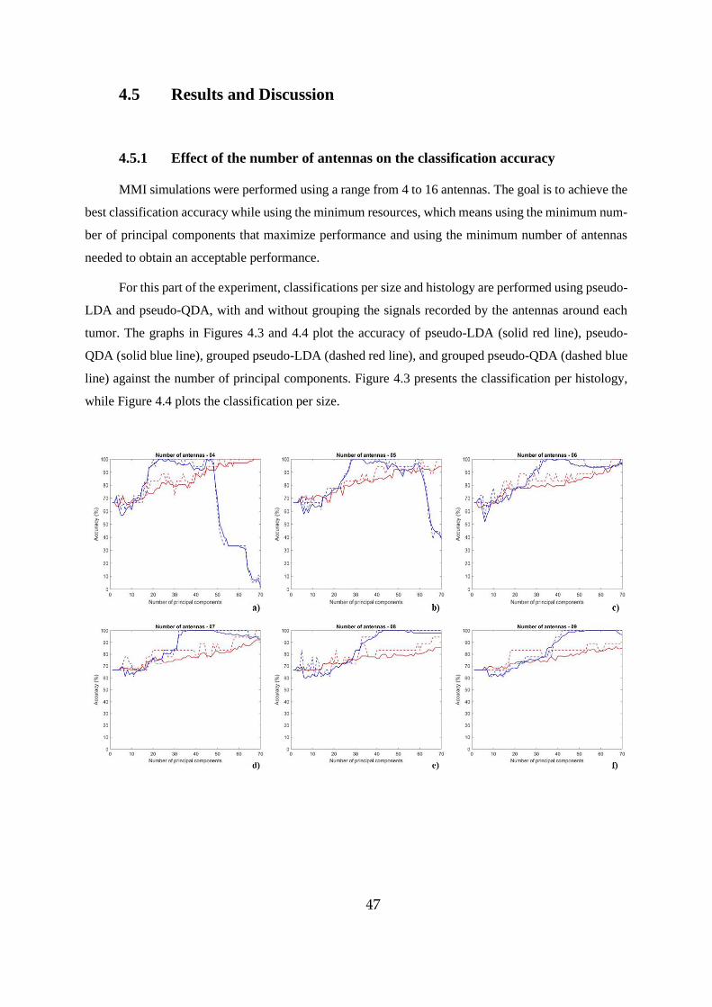
47

4.5 Results and Discussion

4.5.1 Effect of the number of antennas on the classification accuracy

MMI simulations were performed using a range from 4 to 16 antennas. The goal is to achieve the

best classification accuracy while using the minimum resources, which means using the minimum num-

ber of principal components that maximize performance and using the minimum number of antennas

needed to obtain an acceptable performance.

For this part of the experiment, classifications per size and histology are performed using pseudo-

LDA and pseudo-QDA, with and without grouping the signals recorded by the antennas around each

tumor. The graphs in Figures 4.3 and 4.4 plot the accuracy of pseudo-LDA (solid red line), pseudo-

QDA (solid blue line), grouped pseudo-LDA (dashed red line), and grouped pseudo-QDA (dashed blue

line) against the number of principal components. Figure 4.3 presents the classification per histology,

while Figure 4.4 plots the classification per size.

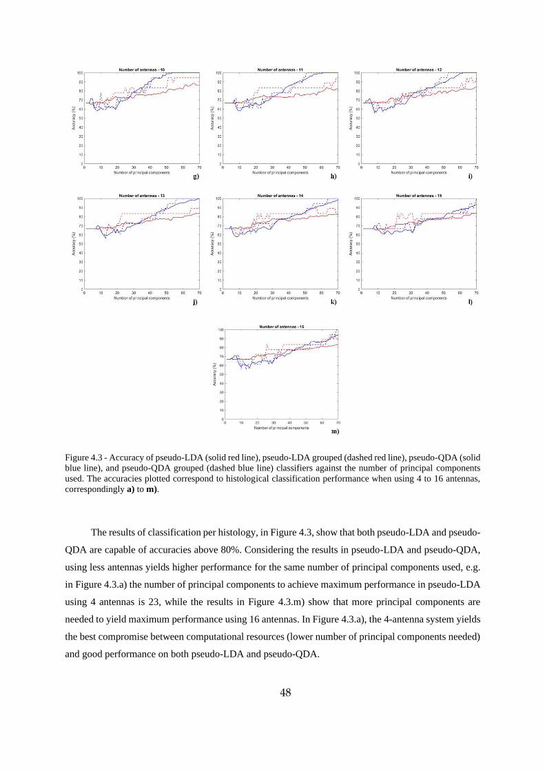
48

Figure 4.3 - Accuracy of pseudo-LDA (solid red line), pseudo-LDA grouped (dashed red line), pseudo-QDA (solid

blue line), and pseudo-QDA grouped (dashed blue line) classifiers against the number of principal components

used. The accuracies plotted correspond to histological classification performance when using 4 to 16 antennas,

correspondingly a) to m).

The results of classification per histology, in Figure 4.3, show that both pseudo-LDA and pseudo-

QDA are capable of accuracies above 80%. Considering the results in pseudo-LDA and pseudo-QDA,

using less antennas yields higher performance for the same number of principal components used, e.g.

in Figure 4.3.a) the number of principal components to achieve maximum performance in pseudo-LDA

using 4 antennas is 23, while the results in Figure 4.3.m) show that more principal components are

needed to yield maximum performance using 16 antennas. In Figure 4.3.a), the 4-antenna system yields

the best compromise between computational resources (lower number of principal components needed)

and good performance on both pseudo-LDA and pseudo-QDA.

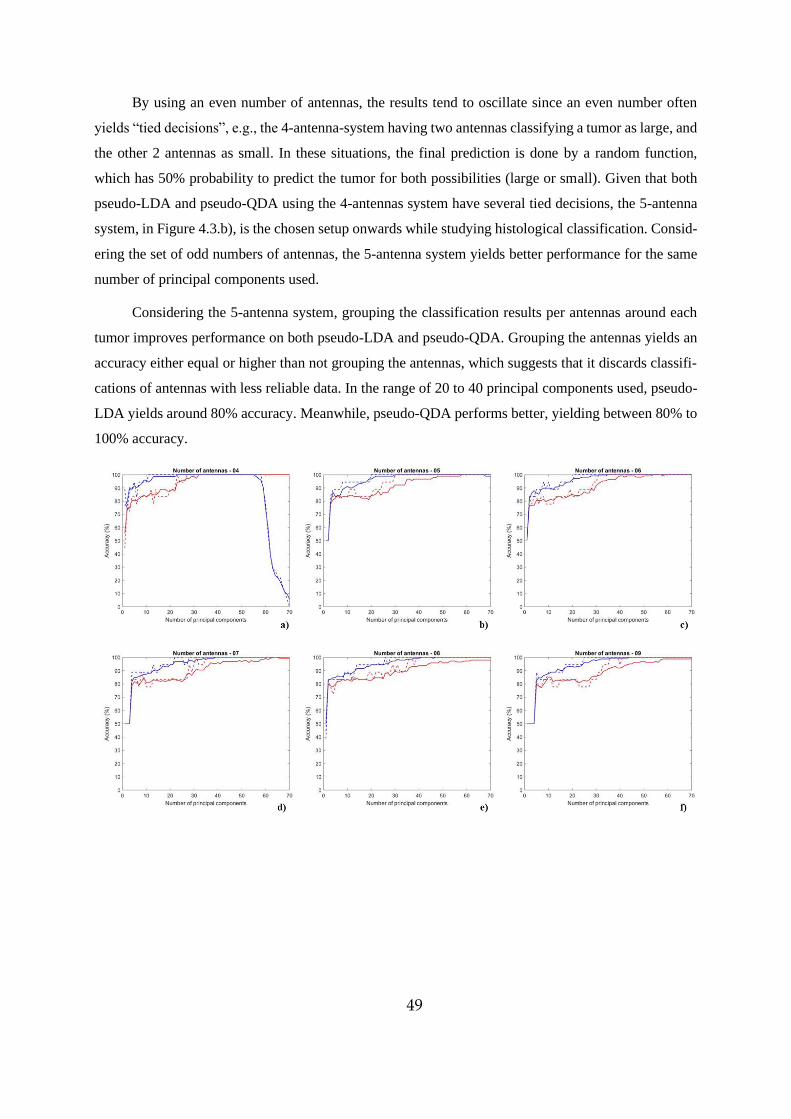
49

By using an even number of antennas, the results tend to oscillate since an even number often

yields “tied decisions”, e.g., the 4-antenna-system having two antennas classifying a tumor as large, and

the other 2 antennas as small. In these situations, the final prediction is done by a random function,

which has 50% probability to predict the tumor for both possibilities (large or small). Given that both

pseudo-LDA and pseudo-QDA using the 4-antennas system have several tied decisions, the 5-antenna

system, in Figure 4.3.b), is the chosen setup onwards while studying histological classification. Consid-

ering the set of odd numbers of antennas, the 5-antenna system yields better performance for the same

number of principal components used.

Considering the 5-antenna system, grouping the classification results per antennas around each

tumor improves performance on both pseudo-LDA and pseudo-QDA. Grouping the antennas yields an

accuracy either equal or higher than not grouping the antennas, which suggests that it discards classifi-

cations of antennas with less reliable data. In the range of 20 to 40 principal components used, pseudo-

LDA yields around 80% accuracy. Meanwhile, pseudo-QDA performs better, yielding between 80% to

100% accuracy.

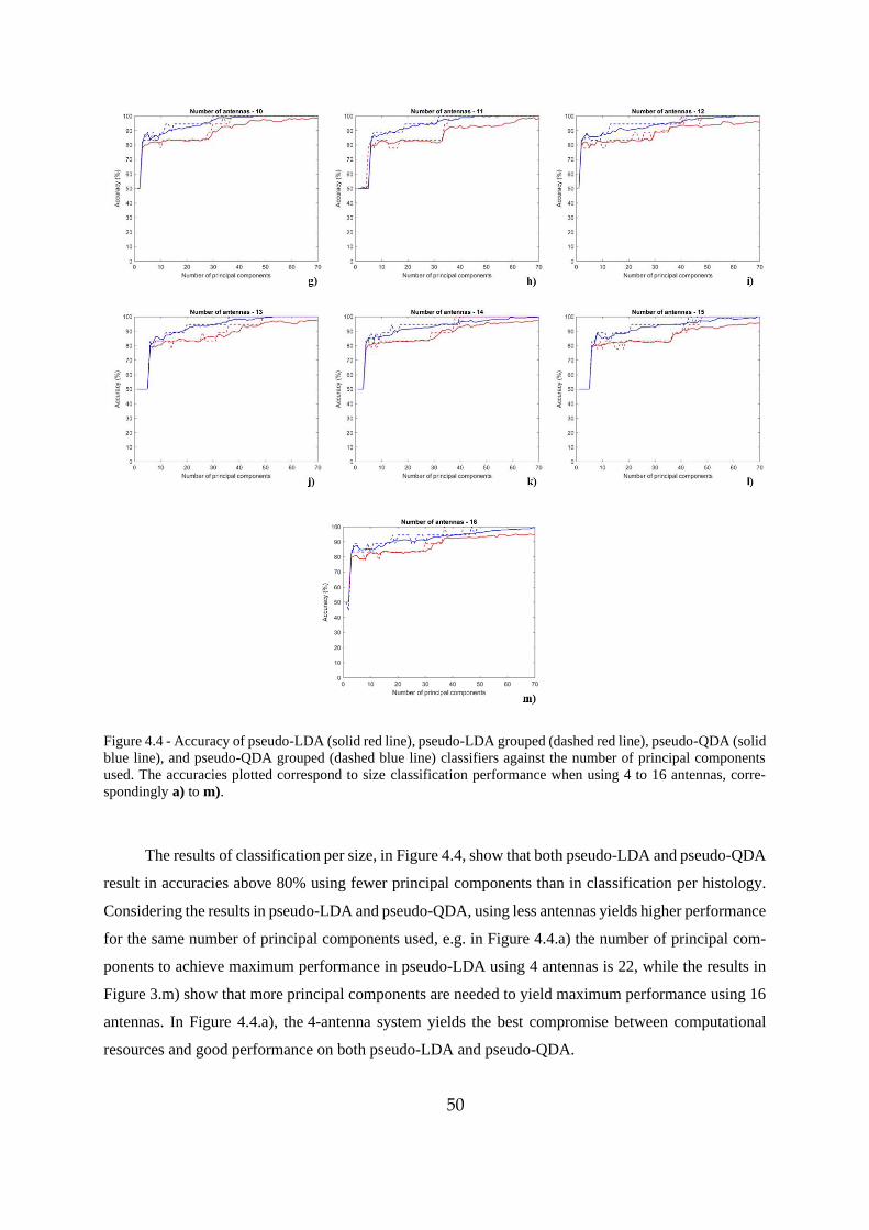
50

Figure 4.4 - Accuracy of pseudo-LDA (solid red line), pseudo-LDA grouped (dashed red line), pseudo-QDA (solid

blue line), and pseudo-QDA grouped (dashed blue line) classifiers against the number of principal components

used. The accuracies plotted correspond to size classification performance when using 4 to 16 antennas, corre-

spondingly a) to m).

The results of classification per size, in Figure 4.4, show that both pseudo-LDA and pseudo-QDA

result in accuracies above 80% using fewer principal components than in classification per histology.

Considering the results in pseudo-LDA and pseudo-QDA, using less antennas yields higher performance

for the same number of principal components used, e.g. in Figure 4.4.a) the number of principal com-

ponents to achieve maximum performance in pseudo-LDA using 4 antennas is 22, while the results in

Figure 3.m) show that more principal components are needed to yield maximum performance using 16

antennas. In Figure 4.4.a), the 4-antenna system yields the best compromise between computational

resources and good performance on both pseudo-LDA and pseudo-QDA.

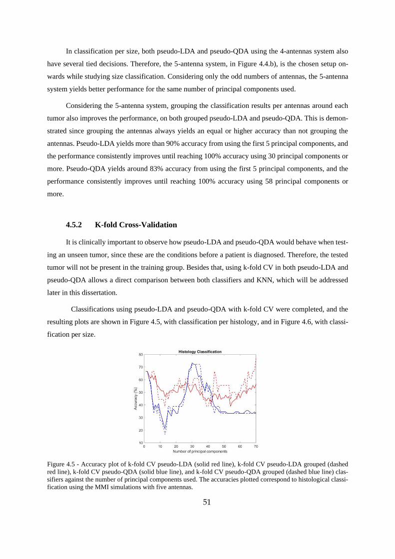
51

In classification per size, both pseudo-LDA and pseudo-QDA using the 4-antennas system also

have several tied decisions. Therefore, the 5-antenna system, in Figure 4.4.b), is the chosen setup on-

wards while studying size classification. Considering only the odd numbers of antennas, the 5-antenna

system yields better performance for the same number of principal components used.

Considering the 5-antenna system, grouping the classification results per antennas around each

tumor also improves the performance, on both grouped pseudo-LDA and pseudo-QDA. This is demon-

strated since grouping the antennas always yields an equal or higher accuracy than not grouping the

antennas. Pseudo-LDA yields more than 90% accuracy from using the first 5 principal components, and

the performance consistently improves until reaching 100% accuracy using 30 principal components or

more. Pseudo-QDA yields around 83% accuracy from using the first 5 principal components, and the

performance consistently improves until reaching 100% accuracy using 58 principal components or

more.

4.5.2 K-fold Cross-Validation

It is clinically important to observe how pseudo-LDA and pseudo-QDA would behave when test-

ing an unseen tumor, since these are the conditions before a patient is diagnosed. Therefore, the tested

tumor will not be present in the training group. Besides that, using k-fold CV in both pseudo-LDA and

pseudo-QDA allows a direct comparison between both classifiers and KNN, which will be addressed

later in this dissertation.

Classifications using pseudo-LDA and pseudo-QDA with k-fold CV were completed, and the

resulting plots are shown in Figure 4.5, with classification per histology, and in Figure 4.6, with classi-

fication per size.

Figure 4.5 - Accuracy plot of k-fold CV pseudo-LDA (solid red line), k-fold CV pseudo-LDA grouped (dashed

red line), k-fold CV pseudo-QDA (solid blue line), and k-fold CV pseudo-QDA grouped (dashed blue line) clas-

sifiers against the number of principal components used. The accuracies plotted correspond to histological classi-

fication using the MMI simulations with five antennas.

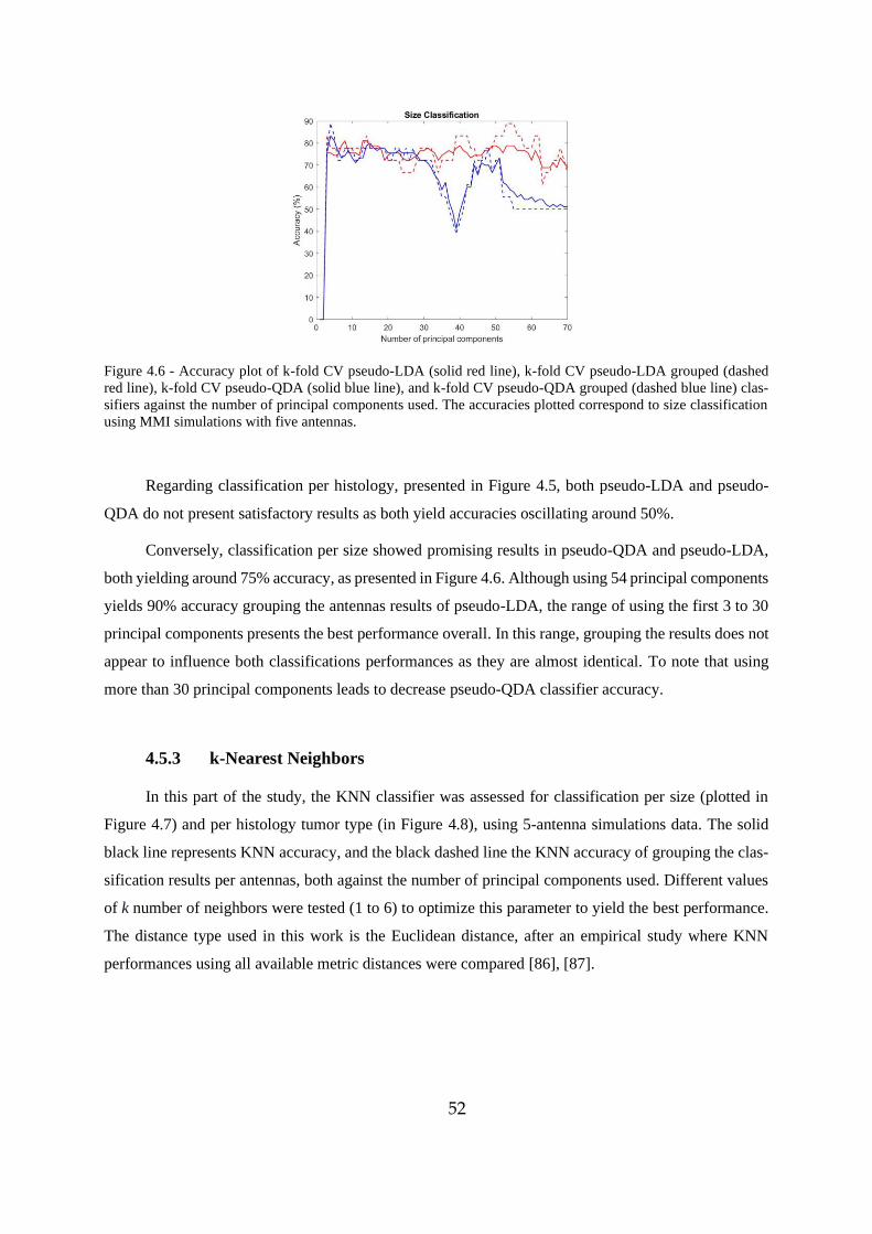
52

Figure 4.6 - Accuracy plot of k-fold CV pseudo-LDA (solid red line), k-fold CV pseudo-LDA grouped (dashed

red line), k-fold CV pseudo-QDA (solid blue line), and k-fold CV pseudo-QDA grouped (dashed blue line) clas-

sifiers against the number of principal components used. The accuracies plotted correspond to size classification

using MMI simulations with five antennas.

Regarding classification per histology, presented in Figure 4.5, both pseudo-LDA and pseudo-

QDA do not present satisfactory results as both yield accuracies oscillating around 50%.

Conversely, classification per size showed promising results in pseudo-QDA and pseudo-LDA,

both yielding around 75% accuracy, as presented in Figure 4.6. Although using 54 principal components

yields 90% accuracy grouping the antennas results of pseudo-LDA, the range of using the first 3 to 30

principal components presents the best performance overall. In this range, grouping the results does not

appear to influence both classifications performances as they are almost identical. To note that using

more than 30 principal components leads to decrease pseudo-QDA classifier accuracy.

4.5.3 k-Nearest Neighbors

In this part of the study, the KNN classifier was assessed for classification per size (plotted in

Figure 4.7) and per histology tumor type (in Figure 4.8), using 5-antenna simulations data. The solid

black line represents KNN accuracy, and the black dashed line the KNN accuracy of grouping the clas-

sification results per antennas, both against the number of principal components used. Different values

of k number of neighbors were tested (1 to 6) to optimize this parameter to yield the best performance.

The distance type used in this work is the Euclidean distance, after an empirical study where KNN

performances using all available metric distances were compared [86], [87].

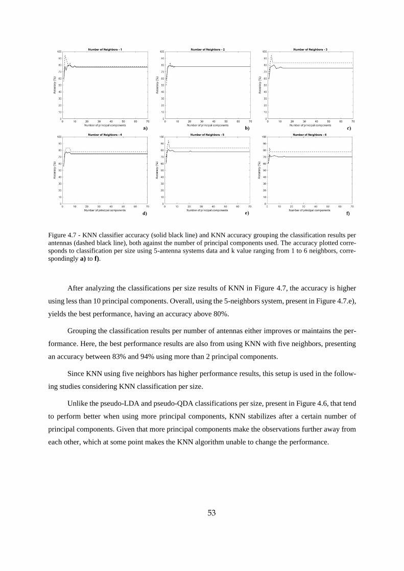
53

Figure 4.7 - KNN classifier accuracy (solid black line) and KNN accuracy grouping the classification results per

antennas (dashed black line), both against the number of principal components used. The accuracy plotted corre-

sponds to classification per size using 5-antenna systems data and k value ranging from 1 to 6 neighbors, corre-

spondingly a) to f).

After analyzing the classifications per size results of KNN in Figure 4.7, the accuracy is higher

using less than 10 principal components. Overall, using the 5-neighbors system, present in Figure 4.7.e),

yields the best performance, having an accuracy above 80%.

Grouping the classification results per number of antennas either improves or maintains the per-

formance. Here, the best performance results are also from using KNN with five neighbors, presenting

an accuracy between 83% and 94% using more than 2 principal components.

Since KNN using five neighbors has higher performance results, this setup is used in the follow-

ing studies considering KNN classification per size.

Unlike the pseudo-LDA and pseudo-QDA classifications per size, present in Figure 4.6, that tend

to perform better when using more principal components, KNN stabilizes after a certain number of

principal components. Given that more principal components make the observations further away from

each other, which at some point makes the KNN algorithm unable to change the performance.

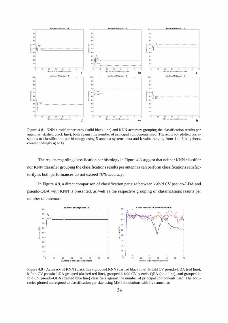
54

Figure 4.8 - KNN classifier accuracy (solid black line) and KNN accuracy grouping the classification results per

antennas (dashed black line), both against the number of principal components used. The accuracy plotted corre-

sponds to classification per histology using 5-antenna systems data and k value ranging from 1 to 6 neighbors,

correspondingly a) to f).

The results regarding classification per histology in Figure 4.8 suggest that neither KNN classifier

nor KNN classifier grouping the classifications results per antennas can perform classifications satisfac-

torily as both performances do not exceed 70% accuracy.

In Figure 4.9, a direct comparison of classification per size between k-fold CV pseudo-LDA and

pseudo-QDA with KNN is presented, as well as the respective grouping of classifications results per

number of antennas.

Figure 4.9 - Accuracy of KNN (black line), grouped KNN (dashed black line), k-fold CV pseudo-LDA (red line),

k-fold CV pseudo-LDA grouped (dashed red line), grouped k-fold CV pseudo-QDA (blue line), and grouped k-

fold CV pseudo-QDA (dashed blue line) classifiers against the number of principal components used. The accu-

racies plotted correspond to classification per size using MMI simulations with five antennas.

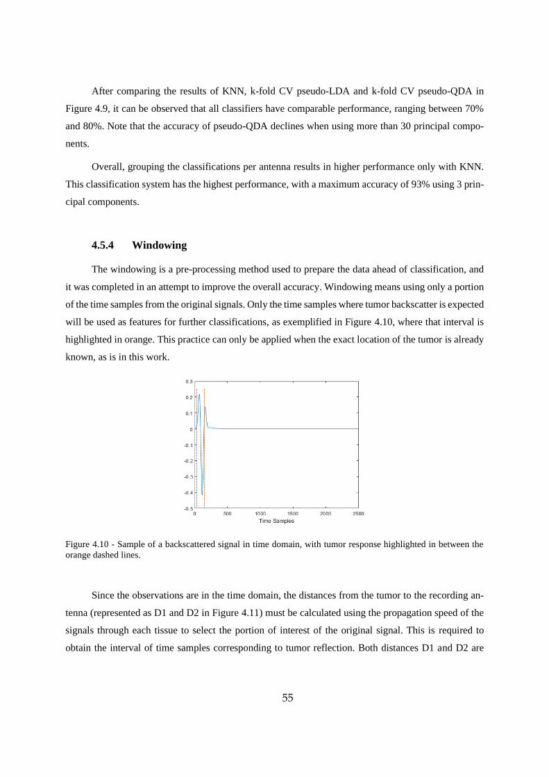
55

After comparing the results of KNN, k-fold CV pseudo-LDA and k-fold CV pseudo-QDA in

Figure 4.9, it can be observed that all classifiers have comparable performance, ranging between 70%

and 80%. Note that the accuracy of pseudo-QDA declines when using more than 30 principal compo-

nents.

Overall, grouping the classifications per antenna results in higher performance only with KNN.

This classification system has the highest performance, with a maximum accuracy of 93% using 3 prin-

cipal components.

4.5.4 Windowing

The windowing is a pre-processing method used to prepare the data ahead of classification, and

it was completed in an attempt to improve the overall accuracy. Windowing means using only a portion

of the time samples from the original signals. Only the time samples where tumor backscatter is expected

will be used as features for further classifications, as exemplified in Figure 4.10, where that interval is

highlighted in orange. This practice can only be applied when the exact location of the tumor is already

known, as is in this work.

Figure 4.10 - Sample of a backscattered signal in time domain, with tumor response highlighted in between the

orange dashed lines.

Since the observations are in the time domain, the distances from the tumor to the recording an-

tenna (represented as D1 and D2 in Figure 4.11) must be calculated using the propagation speed of the

signals through each tissue to select the portion of interest of the original signal. This is required to

obtain the interval of time samples corresponding to tumor reflection. Both distances D1 and D2 are

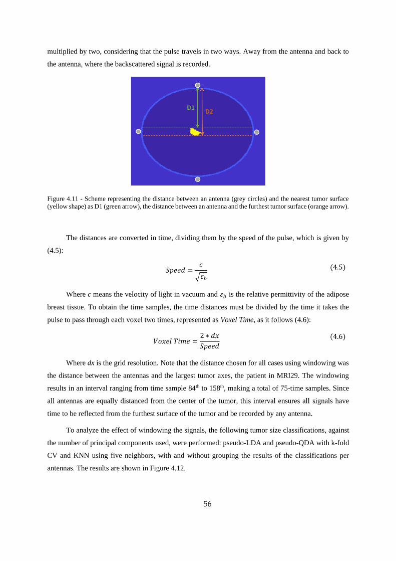
56

multiplied by two, considering that the pulse travels in two ways. Away from the antenna and back to

the antenna, where the backscattered signal is recorded.

Figure 4.11 - Scheme representing the distance between an antenna (grey circles) and the nearest tumor surface

(yellow shape) as D1 (green arrow), the distance between an antenna and the furthest tumor surface (orange arrow).

The distances are converted in time, dividing them by the speed of the pulse, which is given by

(4.5):

𝑆𝑝𝑒𝑒𝑑 =𝑐

√𝜀𝑏

(4.5)

Where c means the velocity of light in vacuum and 𝜀𝑏 is the relative permittivity of the adipose

breast tissue. To obtain the time samples, the time distances must be divided by the time it takes the

pulse to pass through each voxel two times, represented as Voxel Time, as it follows (4.6):

𝑉𝑜𝑥𝑒𝑙 𝑇𝑖𝑚𝑒 =

2 ∗ 𝑑𝑥

𝑆𝑝𝑒𝑒𝑑

(4.6)

Where dx is the grid resolution. Note that the distance chosen for all cases using windowing was

the distance between the antennas and the largest tumor axes, the patient in MRI29. The windowing

results in an interval ranging from time sample 84th to 158th, making a total of 75-time samples. Since

all antennas are equally distanced from the center of the tumor, this interval ensures all signals have

time to be reflected from the furthest surface of the tumor and be recorded by any antenna.

To analyze the effect of windowing the signals, the following tumor size classifications, against

the number of principal components used, were performed: pseudo-LDA and pseudo-QDA with k-fold

CV and KNN using five neighbors, with and without grouping the results of the classifications per

antennas. The results are shown in Figure 4.12.

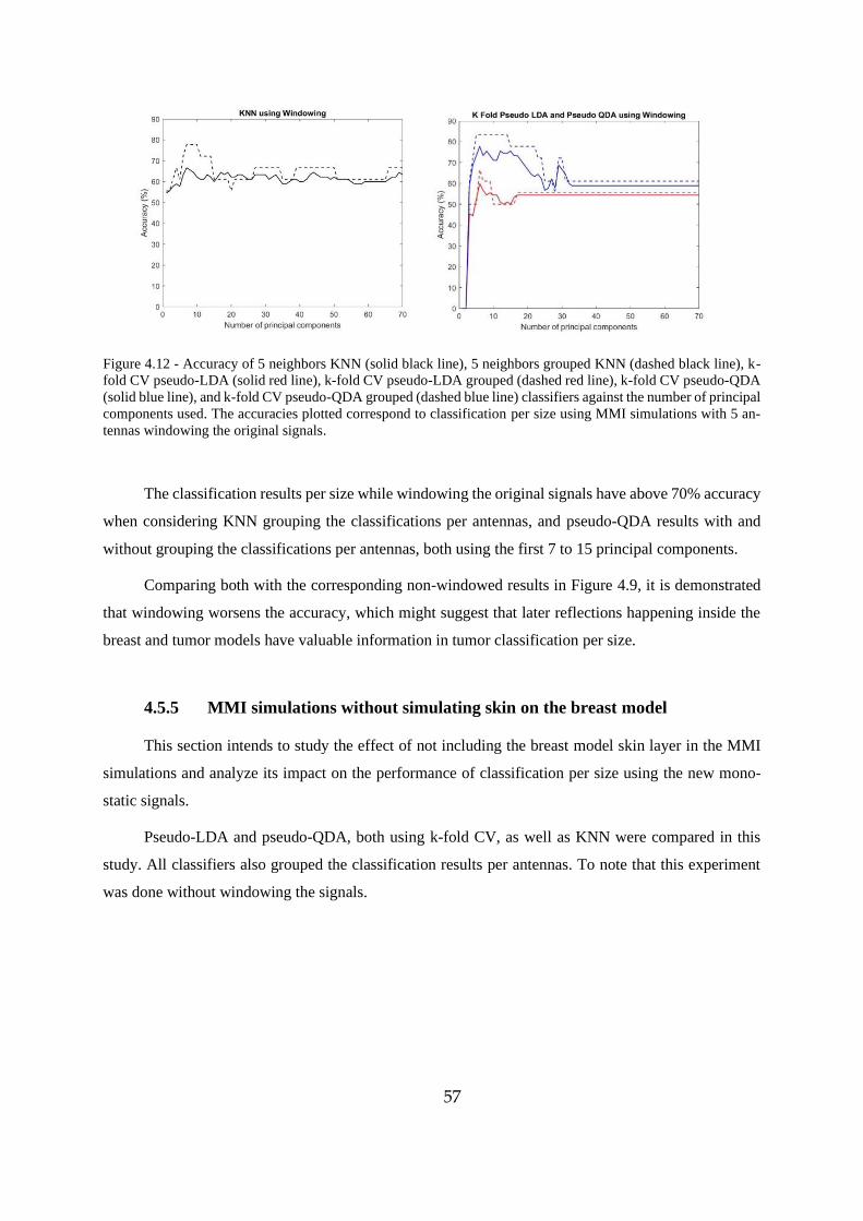
57

Figure 4.12 - Accuracy of 5 neighbors KNN (solid black line), 5 neighbors grouped KNN (dashed black line), k-

fold CV pseudo-LDA (solid red line), k-fold CV pseudo-LDA grouped (dashed red line), k-fold CV pseudo-QDA

(solid blue line), and k-fold CV pseudo-QDA grouped (dashed blue line) classifiers against the number of principal

components used. The accuracies plotted correspond to classification per size using MMI simulations with 5 an-

tennas windowing the original signals.

The classification results per size while windowing the original signals have above 70% accuracy

when considering KNN grouping the classifications per antennas, and pseudo-QDA results with and

without grouping the classifications per antennas, both using the first 7 to 15 principal components.

Comparing both with the corresponding non-windowed results in Figure 4.9, it is demonstrated

that windowing worsens the accuracy, which might suggest that later reflections happening inside the

breast and tumor models have valuable information in tumor classification per size.

4.5.5 MMI simulations without simulating skin on the breast model

This section intends to study the effect of not including the breast model skin layer in the MMI

simulations and analyze its impact on the performance of classification per size using the new mono-

static signals.

Pseudo-LDA and pseudo-QDA, both using k-fold CV, as well as KNN were compared in this

study. All classifiers also grouped the classification results per antennas. To note that this experiment

was done without windowing the signals.

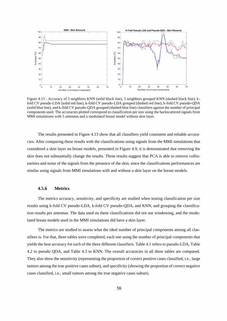
58

Figure 4.13 - Accuracy of 5 neighbors KNN (solid black line), 5 neighbors grouped KNN (dashed black line), k-

fold CV pseudo-LDA (solid red line), k-fold CV pseudo-LDA grouped (dashed red line), k-fold CV pseudo-QDA

(solid blue line), and k-fold CV pseudo-QDA grouped (dashed blue line) classifiers against the number of principal

components used. The accuracies plotted correspond to classification per size using the backscattered signals from

MMI simulations with 5 antennas and a modulated breast model without skin layer.

The results presented in Figure 4.13 show that all classifiers yield consistent and reliable accura-

cies. After comparing these results with the classifications using signals from the MMI simulations that

considered a skin layer on breast models, presented in Figure 4.9, it is demonstrated that removing the

skin does not substantially change the results. These results suggest that PCA is able to remove collin-

earities and noise of the signals from the presence of the skin, since the classifications performances are

similar using signals from MMI simulations with and without a skin layer on the breast models.

4.5.6 Metrics

The metrics accuracy, sensitivity, and specificity are studied when testing classification per size

results using k-fold CV pseudo-LDA, k-fold CV pseudo-QDA, and KNN, and grouping the classifica-

tion results per antennas. The data used on these classifications did not use windowing, and the modu-

lated breast models used in the MMI simulations did have a skin layer.

The metrics are studied to assess what the ideal number of principal components among all clas-

sifiers is. For that, three tables were completed, each one using the number of principal components that

yields the best accuracy for each of the three different classifiers. Table 4.1 refers to pseudo-LDA, Table

4.2 to pseudo QDA, and Table 4.3 to KNN. The overall accuracies in all three tables are compared.

They also show the sensitivity (representing the proportion of correct positive cases classified, i.e., large

tumors among the true positive cases subset), and specificity (showing the proportion of correct negative

cases classified, i.e., small tumors among the true negative cases subset).

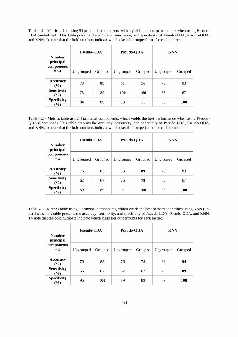
59

Table 4.1 - Metrics table using 54 principal components, which yields the best performance when using Pseudo-

LDA (underlined). This table presents the accuracy, sensitivity, and specificity of Pseudo-LDA, Pseudo-QDA,

and KNN. To note that the bold numbers indicate which classifier outperforms for each metric.

Table 4.2 - Metrics table using 4 principal components, which yields the best performance when using Pseudo-

QDA (underlined). This table presents the accuracy, sensitivity, and specificity of Pseudo-LDA, Pseudo-QDA,

and KNN. To note that the bold numbers indicate which classifier outperforms for each metric.

Table 4.3 - Metrics table using 3 principal components, which yields the best performance when using KNN (un-

derlined). This table presents the accuracy, sensitivity, and specificity of Pseudo-LDA, Pseudo-QDA, and KNN.

To note that the bold numbers indicate which classifier outperforms for each metric.

Number

principal

components

= 54

Pseudo-LDA

Pseudo-QDA

KNN

Ungrouped Grouped Ungrouped Grouped Ungrouped Grouped

Accuracy

(%) 79 89 61 56 78 83

Sensitivity

(%) 73 89 100 100 58 67

Specificity

(%) 84 89 18 11 98 100

Number

principal

components

= 4

Pseudo-LDA

Pseudo-QDA

KNN


Accuracy

(%) 76 83 78 89 79 83

Sensitivity

(%) 62 67 76 78 62 67

Specificity

(%) 89 89 91 100 96 100

Number

principal

components

= 3

Pseudo-LDA

Pseudo-QDA

KNN


Accuracy

(%) 76 83 76 78 81 94

Sensitivity

(%) 56 67 62 67 73 89

Specificity

(%) 96 100 89 89 89 100

60

As presented in Table 4.1, pseudo-LDA yields the best accuracy, 79%, using 54 principal com-

ponents. Grouping classification results per antennas results in higher performance, yielding 89% accu-

racy. Overall using 54 principal components only yields performances above 75% with Pseudo-LDA

and KNN. Regarding sensitivity, pseudo-LDA results are 89%, but amongst all three classifiers, pseudo-

QDA has the highest sensitivity yielding 100% with and without grouping the results per antennas. KNN

has the highest specificity yielding 100% when grouping the results per antennas and 98% without

grouping.

Table 4.2 shows that pseudo-QDA yields the best accuracy using 4 principal components, yield-

ing 78%. Grouping classification results per antennas results in higher performance, yielding 89% ac-

curacy. Using 4 principal components yields overall a similar performance for all classifiers. Regarding

sensitivity, pseudo-QDA results are 76%, and 78% grouping the results per antennas, which are the

highest among all three classifiers. Pseudo-QDA has the highest specificity yielding 100% when group-

ing the results per antennas and 91% without grouping.

Finally, Table 4.3 shows that KNN yields the best accuracy using 3 principal components yielding

81%. Grouping classification results per antennas results in higher performance, yielding 94% accuracy.

Using 3 principal components also yields a similar overall performance in all classifiers. Regarding

sensitivity, KNN results are 73%, and 89% grouping the results per antennas, which are the highest

among all three classifiers. Pseudo LDA has the highest specificity yielding 100% when grouping the

results per antennas and 96% without grouping. To note that KNN also yields 100% specificity when

grouping the results per antennas.

4.6 Chapter Conclusions

This chapter of the dissertation presents the experiments pursued to analyze the radar target sig-

nature of tumor models, classifying them per size and histology type, which in this last case meant as

either an invasive ductal carcinoma or not. Classification per histology considers tumor shape, while

classification per size considers a tumor as large if it has a major axis equal or larger than the median

value among all tumors, or as a small tumor otherwise. The data yielded from the MMI simulations in

chapter 3 was utilized to classify the 2D tumor models, using three classifiers: pseudo-LDA, pseudo-

QDA, and KNN.

The first experiment was two-fold. Assessing the number of antennas necessary to extract

enough information for reliable classifications and assess the performance of pseudo-LDA and pseudo-

QDA as tumor classifiers. These classifications used the training group equal to the testing group since

pseudo-LDA and pseudo-QDA do not overfit.

61

After comparing the graphs in Figures 4.3 and 4.4, it was observed that using 4 antennas in

MMI simulations yields the best compromise between computational resources and performance on

both pseudo-LDA and pseudo-QDA classifications per size and histology. Both classifiers can yield

accuracies higher than 80%, but pseudo-LDA has higher efficiency since it needs less principal compo-

nents to do so.

Grouping the results per number of antennas of pseudo-LDA and pseudo-QDA classifiers was

tested to infer whether it improves the performances, which proved to be true when the number of an-

tennas is odd. Hence, subsequent experiments used the MMI simulations data with 5 antennas, since

amongst the simulations with odd number of antennas, it yields highest performance and efficiency.

Performing k-fold CV was used to assess how pseudo-LDA and pseudo-QDA would behave

when trying to classify a previously unknown tumor, which is the initial condition when a real patient

goes through a diagnostic system. It also allows a direct comparison of these two classifiers with KNN

as it is compulsory to use some form of validation when training a KNN model (to avoid overfitting).

Even though the performances of pseudo-LDA and pseudo-QDA using k-fold CV were lower than not

using it, the classifications per size using k-fold CV pseudo-LDA and k-fold CV pseudo-QDA had sat-

isfactory performance to make them useful in future studies. Meanwhile, classification per histology

type using k-fold CV pseudo-LDA and pseudo-QDA were not satisfactory.

Regarding the KNN classifier, from analyzing and comparing classifications accuracy per size

on six different KNN classification models, using k = 1 to 6 neighbors, the ideal number of neighbors

among those tested is 5, which yields the best performance. Similarly to pseudo-LDA and pseudo-QDA

with k-fold CV, KNN also failed to provide reliable classification results per histology, which might

suggest that the surface and texture information in 2D tumor models is not enough to accurately classify

invasive ductal carcinomas. Another reason might be the large variability of types of tumors that are not

invasive ductal carcinomas. Therefore, only classification per size was investigated in subsequent ex-

periments.

Considering classifications per size, both pseudo-LDA and pseudo-QDA with k-fold CV results

and KNNs using 5 neighbors have similar performances. When considering grouping each classifier

results per antennas, only KNN accuracy results are improved.

The metrics of pseudo-LDA and pseudo-QDA with k-fold CV, and KNNs using 5 neighbors were

analyzed in Tables 4.1, 4.2, and 4.3. They present the number of principal components needed to max-

imize performance for each classifier, showing the accuracy, sensitivity, and specificity. Overall, using

3 to 4 principal components yields the best performance amongst all classifiers, having accuracies above

75%. Regarding sensitivity and specificity, using 3 to 4 principal components, specificity results are

62

better than sensitivity, which indicates that classifying small tumors tends to be more accurate than

classifying large tumors.

Different approaches were followed to potentially improve classification using the MMI simu-

lated data. We attempted windowing the signals and infer the impact that the skin layer has on classify-

ing tumors. The windowing study shows that pseudo-QDA and KNN can classify tumors per size, but

the performances are lower compared to the classifications where signals were not windowed. This

might suggest that using the time-samples recorded after the reflections from the tumor helps improve

classification performance.

Finally, after studying classifications that used the backscattered signals from MMI simulations

using breast tumors without a skin layer, it was concluded that the absence of skin did not impact any

of the performances of the classifications. Proving that, in the conditions of this work, the dielectric

contrast between the skin and breast model does not worsen tumor classification performance per size.

This reinforces that real skin may not interfere with tumor classifications when using patients' MMI

data, although more studies are needed to verify this. Particularly, studies considering breast models

with different shapes and sizes. Given that in the conditions of this work, the breast model is the same

in all simulations, which might ease PCA to discard collinearities and noise of the signals from the

presence of the skin.

63

5 Conclusion

MMI is still being established as a reliable alternative in breast cancer diagnosis. This work has

contributed with the validation of data from MMI simulations recreating a UWB microwave radar im-

aging system to classify breast tumors using classification algorithms. Some of the challenges that this

work and other studies face regarding MMI systems include:

- Difficulty in isolating the tumor response from the recorded backscattered signals. Since the

skin produces artifacts, each woman has different breast anatomy, and the fact that tumors have

unique shapes, sizes and can occur anywhere within the breast, leading to different tumor sig-

natures recorded by exterior antennas.

- Individually, the receiving antennas have a unique view for each tumor, which means each one

records a different tumor signature. Also, if the antennas are at different distances between them

and the tumor, the recorded tumor signature will have different intensities.

- Classification algorithms must be carefully used, so they do not overfit the data recorded by the

antennas [23].

While addressing some of the challenges mentioned, the primary goal of this dissertation is to

further validate that MMI is feasible in clinical scenarios. This work was divided into two objectives,

first creating realistic tumor models from segmenting breast MRI exams, to fit them to 3D printing and

using them in 2D MMI simulations, and secondly use the data acquired in the simulations to classify

tumors in size and histology.

Regarding the first goal, breast tumors were successfully created through manually segmenting

breast tumors from MRI exams, using iSeg and ITK Snap, and a protocol was developed so that future

studies can have a standard procedure to do so. This work segmented seventy-two 3D and eighteen 2D

tumor models from eighteen MRIs. Four different models were created for each tumor, either smoothed

with three smoothing levels (to compensate for the low resolution from the MRIs) and without any

smoothing. Each 2D tumor model was used in different 2D MMI simulations with 4 to 16 antennas,

acquiring the data needed to make the classifications. Regarding the 3D tumor models, these can be 3D

printed and used in future experimental studies.

This part of the work had some limitations, including the challenges from visually distinguish-

ing tumor and healthy breast tissues within the MRI exams. Most of the process was manual, which is

64

more prone to errors. Hence, in the future, dedicated tumor segmentation methodology could use ma-

chine learning techniques, which would require less breast anatomical knowledge from the user and less

prone to human errors.

The second objective of this work was to attempt size and histological tumor classification using

three classification algorithms, pseudo-LDA, pseudo-QDA, and KNN, and a feature extraction algo-

rithm – PCA. The data yielded from the 2D MMI simulations did not have enough information to his-

tologically classify the tumors as invasive ductal carcinomas or not, which indicates that the information

in 2D tumor models is not enough to accurately classify invasive ductal carcinomas. Another reason

might be the large variability of types of tumors that are not invasive ductal carcinomas, including in-

vasive lobular carcinoma, ductal carcinoma in situ, papillary tumor with characteristics of intraductal

papilloma and fibroadenoma, as presented in Table 3.2. Conversely, size classification was well per-

formed using all classifiers. It was concluded that the MMI simulations using less antennas produced

more relevant data to classify tumors, and so all experiments used the 5-antennas system. Pseudo-LDA

and pseudo-QDA used k-fold CV to be tested in a scenario where the tested tumor is not labeled and to

allow a direct comparison with the implementation of KNN.

Using three to four principal components proved to yield the best performance amongst the

classifiers, all with similar results yielding accuracies above 75%. Grouping the antennas results notice-

ably improved KNN performance, achieving an accuracy of 94% with three principal components.

Regarding windowing the tumor signatures from the recorded signals, it was concluded that it

did not improve the classification results.

Lastly, 2D MMI simulations recreating a UWB microwave radar imaging system were repeated

using a numerical breast model without a skin layer to assess the impact on tumor size classification

accuracy. The results with skin were better than those without skin, indicating that skin did not impact

tumor classification per size.

The main limitation of this work was the fact that the MMI simulations had to be performed in

2D instead of 3D making them less realistic. Future work could use the 3D numerical tumors produced

in this dissertation, 3D print them, and alongside with breast phantoms, use them in a UWB microwave

radar imaging prototype to compare the subsequent classification results with this work.

65

6 Bibliography

[1] World Cancer Research Fund, “Worldwide cancer data”.

https://www.wcrf.org/dietandcancer/cancer-trends/worldwide-cancer-data. (accessed Jan. 29,

2020).

[2] H. P. Schlemmer et al., “Global Challenges for Cancer Imaging,” Journal of Global Oncology,

vol. 2018, no. 4, pp. 1–10, 2018.

[3] World Health Organization and International Agency for Research on Cancer, “Cancer Today,”

2020. https://gco.iarc.fr/today/home (accessed Jan. 02, 2021).

[4] M. J. M. Broeders, T. M. Ripping, and R. A. Hubbard, “Weighing the Benefits and Harms,” in

Breast Cancer Screening, N. Houssami and D. Migliorett, Eds. Cambridge: Massachusetts:

Academic Press, 2016, pp. 51–85.

[5] H. D. Nelson, E. S. O’Meara, K. Kerlikowske, S. Balch, and D. Miglioretti, “Factors Associated

with Rates of False-positive and False- negative Results from Digital Mammography Screening:

An Analysis of Registry Data,” Annals of Internal Medicine, vol. 164, no. 4, pp. 226–235, 2016.

[6] I. H. R. Hauge, K. Pedersen, H. M. Olerud, E. O. Hole, and S. Hofvind, “The Risk of Radiation-

induced Breast Cancers due to Biennial Mammographic Screening in Women Aged 50–69 Years

is Minimal,” Acta Radiologica, vol. 55, no. 10, pp. 1174–1179, 2014.

[7] S. J. Lord et al., “A Systematic Review of the Effectiveness of Magnetic Resonance Imaging

(MRI) as an Addition to Mammography and Ultrasound in Screening Young Women at High

Risk of breast cancer,” European Journal of Cancer, vol. 43, no. 13, pp. 1905–1917, 2007.

[8] S. G. Orel and M. D. Schnall, “MR Imaging of the Breast for the Detection, Diagnosis, and

Staging of Breast Cancer,” Radiology, vol. 220, no. 1, pp. 13–30, 2001.

[9] R. Guo, G. Lu, B. Qin, and B. Fei, “Ultrasound Imaging Technologies for Breast Cancer

Detection and Management: A Review,” Ultrasound in Medicine and Biology, vol. 44, no. 1.

Elsevier USA, pp. 37–70, 2018.

[10] J. Shriki, “Ultrasound physics,” Critical Care Clinics, vol. 30, no. 1, pp. 1–24, 2014.

[11] M. A. Aldhaeebi, K. Alzoubi, T. S. Almoneef, S. M. Bamatra, H. Attia, and O. M. Ramahi,

“Review of Microwaves Techniques for Breast Cancer Detection,” Sensors (Switzerland), vol.

20, no. 8, 2020.

[12] A. W. Preece, I. Craddock, M. Shere, L. Jones, and H. L. Winton, “MARIA M4: Clinical

Evaluation of a Prototype Ultrawideband Radar Scanner for Breast Cancer Detection,” Journal

of Medical Imaging, vol. 3, no. 3, p. 033502, 2016.

[13] J. D. Gil Cano, A. Fasoula, L. Duchesne, and J.-G. Bernard, “Wavelia Breast Imaging: The

Optical Breast Contour Detection Subsystem,” Applied Sciences, vol. 10, no. 4, 2020.

[14] B. R. Lavoie, M. Okoniewski, and E. C. Fear, “Estimating the Effective Permittivity for

Reconstructing Accurate Microwave-Radar Images,” PLOS ONE, vol. 11, no. 9, 2016.

[15] J. Bourqui and E. C. Fear, “System for Bulk Dielectric Permittivity Estimation of Breast Tissues

at Microwave Frequencies,” IEEE Transactions on Microwave Theory and Techniques, vol. 64,

no. 9, pp. 3001–3009, 2016.

[16] L. Kranold and M. Popovic, “RF Radar Breast Health Monitoring: System Evaluation with Post-

66

Biopsy Marker,” IEEE Journal of Electromagnetics, RF and Microwaves in Medicine and

Biology, 2020.

[17] Y. Li, E. Porter, A. Santorelli, M. Popović, and M. Coates, “Microwave Breast Cancer Detection

via Cost-Sensitive Ensemble Classifiers: Phantom and Patient Investigation,” Biomedical Signal

Processing and Control, vol. 31, pp. 366–376, 2017.

[18] R. C. Conceição, M. O’Halloran, M. Glavin, and E. Jones, “Numerical Modelling for Ultra

Wideband Radar Breast Cancer Detection and Classification,” Progress In Electromagnetics

Research B, vol. 34, no. 34, pp. 145–171, 2011.

[19] R. C. Conceição, M. O’Halloran, E. Jones, and M. Glavin, “Investigation of Classifiers for Early-

Stage Breast Cancer Based on Radar Target Signatures,” Progress in Electromagnetics

Research, vol. 105, pp. 295–311, 2010.

[20] R. C. Conceiçao, M. O’Halloran, M. Glavin, and E. Jones, “Support Vector Machines for the

Classification of Early-Stage Breast Cancer Based on Radar Target Signatures,” Progress In

Electromagnetics Research B, vol. 23, no. 23, pp. 311–327, 2010.

[21] R. C. Conceição et al., “Classification of Breast Tumor Models with a Prototype Microwave

Imaging System,” Medical Physics, vol. 47, no. 4, pp. 1860–1870, 2020.

[22] B. L. Oliveira et al., “Combined Breast Microwave Imaging and Diagnosis System,” in Progress

In Electromagnetics Research Symposium (PIERS). Prague, Czech Republic, 2015, pp. 274–

278, [Online]. Available: https://www.researchgate.net/publication/285429704.

[23] B. Oliveira, D. Godinho, M. O’Halloran, M. Glavin, E. Jones, and R. Conceição, “Diagnosing

Breast Cancer with Microwave Technology: remaining challenges and potential solutions with

machine learning,” Diagnostics, vol. 8, no. 2, p. 36, 2018.

[24] K. Muinonen, “Introducing the Gaussian Shape Hypothesis for Asteroids and Comets,”

Astronomy Astrophysics, vol. 332, pp. 1087–1098, 1998.

[25] L. T. Michael Mishchenko, Joachim Hovenier, Light Scattering by Nonspherical Particles

Theory, Measurements, and Applications. New York: Academic Press, 1999.

[26] B. L. Oliveira, M. O’Halloran, R. Conceicao, M. Glavin, and E. Jones, “Development of

Clinically Informed 3-D Tumor Models for Microwave Imaging Applications,” IEEE Antennas

and Wireless Propagation Letters, vol. 15, pp. 520–523, 2016.

[27] Y. Chen, E. Gunawan, K. S. Low, S. C. Wang, C. B. Soh, and T. C. Putti, “Effect of Lesion

Morphology on Microwave Signature in 2-D Ultra-Wideband Breast Imaging,” IEEE

Transactions on Biomedical Engineering, vol. 55, no. 8, pp. 2011–2021, 2008.

[28] B. L. Oliveira, D. O’Loughlin, M. O’Halloran, E. Porter, M. Glavin, and E. Jones, “Microwave

Breast Imaging: Experimental Tumour Phantoms for the Evaluation of New Breast Cancer

Diagnosis Systems,” Biomedical Physics and Engineering Express, vol. 4, no. 2, 2018.

[29] E. Zastrow, S. K. Davis, M. Lazebnik, F. Kelcz, B. D. V. Veen, and S. C. Hagness,

“Development of anatomically realistic numerical breast phantoms with accurate dielectric

properties for modeling microwave interactions with the human breast,” IEEE Transactions on

Biomedical Engineering, vol. 55, no. 12, pp. 2792–2800, 2008.

[30] L. Breiman, “Random forests,” Machine Learning, vol. 45, no. 1, pp. 5–32, 2001.

[31] A. Fasoula et al., “Pilot Patient Study with the Wavelia Microwave Breast Imaging System For

Breast Cancer Detection: Clinical Feasibility and Identified Technical Challenges” in 14th

European Conference on Antennas and Propagation, EuCAP 2020. Copenhagen, Denmark,

2020, pp. 1–5, [Online]. Available: https://www.researchgate.net/publication/342797469.

[32] Micrima, “Micrima – Developing technology for breast cancer screening,” 2021.

67

https://micrima.com/ (accessed Jan. 05, 2021).

[33] S. Pandya and R. G. Moore, “Breast Development and Anatomy,” Clinical Obstetrics &

Gynecology, vol. 54, no. 1, pp. 91–95, 2011.

[34] American College of Radiology, “ACR BI-RADS breast imaging and reporting data system :

breast imaging atlas.,” ACR BI-RADS® Atlas - Mammography, 2013.

https://www.acr.org/Clinical-Resources/Reporting-and-Data-Systems/Bi-Rads (accessed Feb.

17, 2021).

[35] R. C. Conceição, J. J. Mohr, and M. O’Halloran, An Introduction to Microwave Imaging for

Breast Cancer Detection. Switzerland: Springer International Publishing, 2016.

[36] M. Patel, “Breast Anatomy.” https://www.slideshare.net/MayurPatel64/breast-anatomy-

151323294 (accessed Sep. 10, 2020).

[37] Breastcancer.org, “Non-Invasive or Invasive Breast Cancer”.

https://www.breastcancer.org/symptoms/diagnosis/invasive (accessed Sep. 30, 2020).

[38] American Cancer Society, “Invasive Breast Cancer (IDC/ILC)”.

https://www.cancer.org/cancer/breast-cancer/understanding-a-breast-cancer-diagnosis/types-of-

breast-cancer/invasive-breast-cancer.html (accessed Oct. 12, 2020).

[39] D. Miklavčič, N. Pavšelj, and F. X. Hart, “Electric Properties of Tissues,” in Wiley Encyclopedia

of Biomedical Engineering, Hoboken, NJ, USA: John Wiley & Sons, Inc., 2006, pp. 3578–3589.

[40] R. C. Conceição, M. O’Halloran, M. Glavin, and E. Jones, “Comparison of planar and circular

antenna configurations for breast cancer detection using microwave imaging,” Progress in

Electromagnetics Research, vol. 99, no. 1, pp. 1–20, 2009.

[41] E. C. Fear, “Microwave imaging of the breast,” in Technology in Cancer Research and

Treatment, 2005, vol. 4, no. 1, pp. 69–82.

[42] Y. Cheng and M. Fu, “Dielectric properties for non-invasive detection of normal, benign, and

malignant breast tissues using microwave theories,” Thoracic Cancer, vol. 9, no. 4, pp. 459–465,

2018.

[43] Microwaves101, “Microwave Medical Applications”.

https://www.microwaves101.com/encyclopedias/microwave-medical-applications (accessed

Nov. 05, 2020).

[44] E. C. Fear, J. Bourqui, C. Curtis, D. Mew, B. Docktor, and C. Romano, “Microwave breast

imaging with a monostatic radar-based system: A study of application to patients,” IEEE

Transactions on Microwave Theory and Techniques, vol. 61, no. 5, pp. 2119–2128, 2013.

[45] E. C. Fear, L. Xu, S. C. Hagness, and M. A. Stuchly, “Confocal Microwave Imaging for Breast

Cancer Detection: Localization of Tumors in Three Dimensions,” IEEE Transactions On

Biomedical Engineering, vol. 49, no. 8, pp. 812–822, 2002.

[46] X. Li, S. K. Davis, S. C. Hagness, D. W. Van Der Weide, and B. D. Van Veen, “Microwave

imaging via space-time beamforming: Experimental investigation of tumor detection in

multilayer breast phantoms,” IEEE Transactions on Microwave Theory and Techniques, vol. 52,

no. 8, pp. 1856–1865, 2004.

[47] I. J. Craddock, R. Nilavalan, J. Leendertz, A. Preece, and R. Benjamin, “Experimental

investigation of real aperture synthetically organised radar for breast cancer detection,” in 2005

IEEE Antennas and Propagation Society International Symposium, 2005, vol. 1B, pp. 179–182,

doi: 10.1109/APS.2005.1551515.

[48] M. Klemm, J. A. Leendertz, D. Gibbins, I. J. Craddock, A. Preece, and R. Benjamin, “Microwave

radar-based breast cancer detection: Imaging in inhomogeneous breast phantoms,” IEEE

68

Antennas and Wireless Propagation Letters, vol. 8, pp. 1349–1352, 2009.

[49] R. Nilavalan, A. Gbedemah, I. J. Craddock, X. Li, and S. C. Hagness, “Numerical investigation

of breast tumour detection using multi-static radar,” Electronics Letters, vol. 39, no. 25, pp.

1787–1789, 2003.

[50] M. Lazebnik et al., “A Large-Scale Study of the Ultrawideband Microwave Dielectric Properties

of Normal Breast Tissue Obtained from Reduction Surgeries,” Physics in Medicine and Biology,

vol. 52, no. 20, pp. 6093–6115, 2007.

[51] R. C. Conceição, M. O’Halloran, M. Glavin, and E. Jones, “Evaluation of features and classifiers

for classification of early-stage breast cancer,” Journal of Electromagnetic Waves and

Applications, vol. 25, no. 1, pp. 1–14, 2011.

[52] R. C. Conceição, M. O’Halloran, M. Glavin, and E. Jones, “Effects of dielectric heterogeneity

in the performance of breast tumour classifiers,” Progress In Electromagnetics Research M, vol.

17, pp. 73–86, 2011.

[53] R. C. da Conceição, “The Development of Ultra Wideband Scanning Techniques for Detection

and Classification of Breast Cancer,” A dissertation presented to The College of Engineering and

Informatics National University of Ireland Galway in fulfilment of the requirements for the

degree of Doctor in the subject of Electrical & Electronic Engineering, Galway, 2010.

[54] M. Lazebnik, M. Okoniewski, J. H. Booske, and S. C. Hagness, “Highly accurate debye models

for normal and malignant breast tissue dielectric properties at microwave frequencies,” IEEE

Microwave and Wireless Components Letters, vol. 17, no. 12, pp. 822–824, 2007.

[55] A. Taflove and S. C. Hagness, Computational Electrodynamics The Finite-Difference Time-

Domain Method, 3rd ed. Boston, MA: Artech House Publishers, 2005.

[56] M. Okoniewski, M. Mrozowski, and M. A. Stuchly, “Simple treatment of multi-term dispersion

in FDTD,” IEEE Microwave and Guided Wave Letters, vol. 7, no. 5, pp. 121–123, 1997.

[57] S. Gabriel, R. W. Lau, and C. Gabriel, “The dielectric properties of biological tissues: III.

Parametric models for the dielectric spectrum of tissues,” Physics in Medicine and Biology, vol.

41, no. 11, pp. 2271–2293, 1996.

[58] Zurich Med Tech ZMT, “Medical Image Segmentation Tool Set,” 2020.

https://zmt.swiss/sim4life/modules/iSeg (accessed Dec. 02, 2020).

[59] P. Yushkevich and G. Gerig, “ITK-SNAP,” 2018. http://www.itksnap.org/pmwiki/pmwiki.php

(accessed Aug. 28, 2020).

[60] C. E. Cardenas, J. Yang, B. M. Anderson, L. E. Court, and K. B. Brock, “Advances in Auto-

Segmentation,” Seminars in Radiation Oncology, vol. 29, no. 3. W.B. Saunders, pp. 185–197,

2019.

[61] O. Sorkine, “Laplacian Mesh Processing,” in EUROGRAPHICS STARs, 2005, pp. 53–70, doi:

10.2312/egst.20051044.

[62] A. Adam, “Mesh voxelisation,” 2021.

https://www.mathworks.com/matlabcentral/fileexchange/27390-mesh-voxelisation (accessed

Sep. 30, 2020).

[63] D. M. Sullivan, Electromagnetic Simulation Using the FDTD Method. New York: Wiley-IEEE

Press, 2000.

[64] S. K. Davis, H. Tandradinata, S. C. Hagness, and B. D. Van Veen, “Ultrawideband microwave

breast cancer detection: A detection-theoretic approach using the generalized likelihood ratio

test,” IEEE Transactions on Biomedical Engineering, vol. 52, no. 7, pp. 1237–1250, 2005.

[65] E. Zastrow, S. K. Davis, M. Lazebnik, F. Kelcz, B. D. Van Veen, and S. C. Hagness, “Database

69

of 3D Grid-Based Numerical Breast Phantoms for use in Computational Electromagnetics

Simulations,” Igarss 2014. Québec, Canada, pp. 1–5, 2014.

[66] M. J. Burfeindt et al., “MRI-derived 3-D-printed breast phantom for microwave breast imaging

validation,” IEEE Antennas and Wireless Propagation Letters, vol. 11, pp. 1610–1613, 2012.

[67] I. J. Craddock, M. Klemm, J. Leendertz, A. W. Preece, and R. Benjamin, “Development and

application of a UWB radar system for breast imaging,” Proceedings of the Loughborough

Antennas and Propagation Conference (LAPC ’08). Loughborough, UK, pp. 24–27, 2008.

[68] J. Bourqui, J. M. Sill, and E. C. Fear, “A prototype system for measuring microwave frequency

reflections from the breast,” International Journal of Biomedical Imaging, vol. 2012, p. 12, 2012.

[69] M. Klemm, I. J. Craddock, J. A. Leendertz, A. Preece, and R. Benjamin, “Radar-based breast

cancer detection using a hemispherical antenna array - Experimental results,” IEEE Transactions

on Antennas and Propagation, vol. 57, no. 6, pp. 1692–1704, 2009.

[70] G. James, D. Witten, T. Hastie, and R. Tibshirani, An Introduction to Statistical Learning.

Stanford: Springer Publishing Company, Incorporated, 2014.

[71] Pier Paolo Ippolito, “Feature Extraction Techniques”. https://towardsdatascience.com/feature-

extraction-techniques-d619b56e31be (accessed Sep. 18, 2020).

[72] J. Shlens, “A Tutorial On Principal Component Analysis,” 2003. [Online]. Available:

arXiv:1404.1100.

[73] M. Ringnér, “What is principal component analysis?,” Nature Biotechnology, vol. 26, no. 3, pp.

303–304, 2008.

[74] I. T. Jollife and J. Cadima, “Principal component analysis: A review and recent developments,”

Philosophical Transactions of the Royal Society A: Mathematical, Physical and Engineering

Sciences, vol. 374, no. 2065, 2016.

[75] G. Bindu, A. Lonappan, V. Thomas, C. K. Aanandan, K. T. Mathew, and S. J. Abraham, “Active

microwave imaging for breast cancer detection,” Progress in Electromagnetics Research, vol.

58, pp. 149–169, 2006.

[76] P. T. Huynh, A. M. Jarolimek, and S. Daye, “The False-negative Mammogram,” Radiographics,

vol. 18, no. 5, pp. 1137–1154, 1998.

[77] K. Rosenberg, “Ten-year risk of false positive screening mammograms and clinical breast

examinations.,” Journal of Nurse-Midwifery, vol. 43, no. 5. pp. 394–395, 1998.

[78] A. M. Martinez and A. C. Kak, “PCA versus LDA,” IEEE Transactions on Pattern Analysis and

Machine Intelligence, vol. 23, no. 2, pp. 228–233, 2001.

[79] G. A. F. Seber, Multivariate Observations. Hoboken, NJ, USA: John Wiley & Sons, Inc., 1984.

[80] T. Raykov and G. A. Marcoulides, An Introduction to applied multivariate analysis. New York:

Routledge Taylor & Francis Group, 2008.

[81] B. S. Everitt, G. Dunn, B. S. Everitt, and G. Dunn, “Multivariate Data and Multivariate

Statistics,” in Applied Multivariate Data Analysis, John Wiley & Sons, Ltd., 2013, pp. 1–8.

[82] W. Wu et al., “Comparison of regularized discriminant analysis, linear discriminant analysis and

quadratic discriminant analysis, applied to NIR data,” Analytica Chimica Acta, vol. 329, no. 3,

pp. 257–265, 1996.

[83] MathWorks, “Improving Discriminant Analysis Models - MATLAB & Simulink”.

https://www.mathworks.com/help/stats/improving-discriminant-analysis-models.html

(accessed Oct. 15, 2020).

[84] Z. Zhang, “Introduction to machine learning: K-nearest neighbors,” Annals of Translational

70

Medicine, vol. 4, no. 11, p. 218, 2016.

[85] T. Hastie, R. Tibshirani, and J. Friedman, The Elements of Statistical Learning. New York:

Springer Nature, 2009.

[86] K. Chomboon, P. Chujai, P. Teerarassamee, K. Kerdprasop, and N. Kerdprasop, “An Empirical

Study of Distance Metrics for k-Nearest Neighbor Algorithm,” The 3rd International Conference

on Industrial Application Engineering ICIAE 2015. Kitakyushu, Japan, 2015.

[87] K. Fukunaga, “The Optimal Distance Measure for Nearest Neighbor Classification,” IEEE

Transactions on Information Theory, vol. 27, no. 5, pp. 622–627, 1981.

Imaging - run.unl.pt

Documents

Transcript of Imaging - run.unl.pt