GRADIÔMETROS SUPERCONDUTORES ACOPLADOS A SQUIDs E … · 1.1 - Biomagnetismo • o conceito de que...

Universidade de São PauloInstituto de Física e Química de São Carlos

Departamento de Física e Ciência dos Materiais

GRADIÔMETROS SUPERCONDUTORES

ACOPLADOS A SQUIDs

E SUA APLICAÇAO EM BIOMAGNETISMO

Antonio Carlos Oliveira Bruno

Tese apresentada ao Instituto de Física e Química de São Carlos

da Universidade de São Paulo para obtenção do título de

Doutor em Ciências - "Física Aplicadi"

Orientador: Paulo Edmundo de Leers Costa Ribeiro

.(Ji6

SUVICO OEBlBLlOTECi; Ê~NfÕR~;AÇAO _ "a-seiL FfSICA

'. )

UNIVERSIDADE DE SÃo PAULOINSTITUTO DE FfSIC~ E QUfMICA DE SÃO CARLOSMEMEROS DR CDMISSRD JULGRDORR DR TESE DE DOUTORRDO DERNTONIO CRRLOS OLIVEIRR ERUNO RPRESENTRDR RO INSTITUTO DE

FISICR E aUIMICR DE SRO CRRLOS,DR UNIVERSIDRDE DE SRO PRULOjEM13 DE SETEMBRO DE 1890.

COMISSRO JULGRDORR:

Prof.Dr.Paul0 E.de L.Costa Ribeiro

~\\---7· .--- -- ----JJ~)_~ ~ ~_--Prof.Dr.HoracloU:arlos Panepuccl

Cx. Postal, 369 - FONE (0162) 71·1016· CEP 13.560' São Carlos . SP - Telex 162374· FOSC - BR - BRASI L

Aos meus pais.

AGRADECIMENTOS

Gostaria de agradecer em primeiro lugar ao Prof. Sergio Mascarenhas quedesde a minha infância me estimulou e me incentivou com seu exemplo, a adentrarnas lides científicas. Como ele gost~de dizer, eu acabei tentando conjugar o verboser. Também foi ele que em meados de 1979 me apresentou ao Prof. Paulo CostaRibeiro que me orientou neste trabalho.

Ao Paulo meu orientador e amigo, agradeço por estes mais de dez anos deconvívio com um otimismo diário, com a crítica sempre construtiva e por ter acreditad~ em mim e neste projeto.

Desejo agradecer também a Profa. Yvonne Mascarenhas e ao Prof. JanSlaets por todo empenho, interesse e hospitalidade sem o que esta tese não teriase concretizado.

A todos que contribuiram com idéias, sugestões e me ajudaram nas experiências, vão os meus agradecimentos: Prof. Bruno Maffeo, Eng. Iradj R.Eghrari, Prof. Jean Piere von der Weid, Dr. Carley C. Paulsen, Enga. AdrianaV. Guida, Sergei D. Soarez e Clarissa Dolce da Silva. Agradecimentos especiaisvão também para Don Antonio P. Picon e Edson (Cidadão) Joaquim da oficinamecânica do Departamento de Física da PUC-Rio.

Desejo tamoém agradecer ao Prof. Orest G. Sym.ko que sempre me incentivoue encorajou a transformar estas publicações em uma tese e especialmente ao Dr.James E. Zimmerman que me ensinou que a arte de fazer SQUIDs pode ser umacoisa simples e divertida.

Agradecimentos são devidos também a todos que especificamente contribuiram para tornar possível o meu estágio de pré-doutoramento na Italia, Prof. SergioMascarenhas, Prof. Paulo Costa Ribeiro, Prof. Sergio Costa Ribeiro, Sonia Nolesco e Prof. Carlos Alberto Aragão de Carvalho.

Um agradecimento especial vai também para todo o pessoal do Istituto diElettronica dello Stato Solido - Consiglio Nazionale delle Ricerche (CNR), Roma,ltalia, pela hospitalidade durante o ano que passei lá, aonde foram realizados ostestes com os gradiômetros planares e a maior parte desta tese foi escrita; Prof.Gian Luca Romani, Dr. Guido Torrioli, Dr. Vittorio Pizzella, Dr. Roberto Leoni,Dr. Sandro Barbanera, Dr. Carlo Salustri, Prof. Ivo Modena e Prof. PasqualinoCarelli que gentilmente permitiu que eu usasse o seu HP- VECTRA aonde eu pudeme iniciar nos mistérios do T:EX typesetting system no qual esta tese foi escrita.

Finalmente desejo agradecer demais a minha esposa Cristiana e ao meu filhoEduardo pelo constante apoio, companheirismo e paciência durante todos estesanos.

Rio de Janeiro, 9 de julho de 1990.

11 -

- - ~- .. _._.-,,-- ..~.,----,,_•..- ..

SERViÇO DE 8IBLh.JTECA E j;'j")d,'.!\çA'J IFOSe!

ffsrCA

,SUMARIO

,PREFACIO 1

_m ~~_

1 INTRODUÇÃO 3

1.1 - Biomagnetismo 31.2 - Campos Biomagnéticos e Ruído Ambiental 4

1.3 - SQUIDs e Discriminação Espacial 5

2 GRADIÔMETROS AXIAIS 8

2.1 - Caracterização Usando a Expanção de Taylor 8

2.2 - Aspectos Práticos na Construção de Gradiômetros 13

2.3 - Testes de Performance e Calibração 15

3 FILTROS ESPACIAIS 19

3.1 - Caracterização Usando a Transformada de Fourier 19

3.2 - Projeto de Filtros Espaciais 23

3.3 - Medida da Função de Transferência 25

3.4 - Calibração 28

4 GRADIÔMETROS PLANARES 31

4.1 - O Gradiômetro Planar como um Filtro Espacial 31

4.2 - Projeto de Arrays 32

4.3 - Recuperação do Sinal de Entrada- 36

5-

DISCUSSAO 38

5.1 - Perspectivas , 385.1 - Conclusão 39

iii

6 PUBLICAÇÕES 40

6.1 - Lista de Publicações 40

6.2 - Resumo das Publicações 41

REFERÊNCIAS

ANEXOS

IV

44

51

,PREFACIO

A detecção de campos biomagnéticos está r~lacionada, à possibilidade demedida de um campo magnético muito fraco imerso em um ambiente magneticamente ruidoso. Uma das fontes responsáveis pela presença de campos magnéticos

no corpo humano, são os deslocamentos iônicos dentro e fora da membrana de

células excitáveis. O ruído magnético provém de varias fontes, como por ex

emplo, o campo magnético terrestre, com um valor aproximadamente um milhãode vezes mais intenso que o mais intenso dos campos biomagnéticos, o campomagnético cardíaco.

O único dispositivo com sensibilidade apropriada para detecção de campos

biomagnéticos é o SQUID (Superconducting QUantum Interference Device). Devido a sua sensibilidade e característica, o SQUID é utilizado em conjunto com

um transformador de fluxo de geometria gradiométrica, que é capaz de discriminar. -

espacialmente fontes distantes (ruído) em favor de fontes próximas ao sensor (sinal

biomagnético) .

O objetivo principal deste trabalho, foi o estudo da discriminação espa

cial realizada através da utilização de gradiômetros, na detecção de campos bio

magnéticos. Esta tese é o produto de um trabalho de pesquisa, que resultou em 12publicações, que apresentam e discutem uma nova abordagem para 'a compreensão

da atuação dos gradiômetros sobre os sinais detectados. Além disso, esta nova

abordagem gerou outras técnicas relevantes para a área, como a calibração do sis

tema com uma precisão até então não alcançada, a possibilidade de recuperaçãodo sinal original detectado e um procedimento para auxiliar o projeto de arrays

de gradiômetros planares.

Esta tese foi escrita de tal forma -que todas as técnicas desenvo~vidas,re

sultados e as principais conclusões estão contidas em seu corpo. Portanto, não énecessária a leitura das publicações, a não ser que um maior aprofundamento emalguns dos assuntos abordados seja desejado. As contribuições específicas dadaspor esta tese serão referenciadas sob forma de anexos. Na introdução, aspectos

gerais de biomagnetismo são discutidos, como também o seu desenvolvimento a

partir da invenção do SQUID. No capítulo 2, estão descritos o modelo convencional, a construção, a medida de performance, a calibraçã.oe aspectos práticos no

projeto de um gradiômetro axial. Detalhes adicionais podem ser encontrados na

1

publicação [1]. No capítulo 3, um novo modelo para gradiômetros é introduzido

baseado em conceitos de filtragem digital e o procedimento da calibração do sis

tema é rediscutido. Detalhes adicionais podem ser encontrados nas publicações [2],

[3], [4], [5], [10] e [12]. No capítulo 4, este modelo é estendido para gradiômetros

planares e é desenvolvido um algorítmo de desconvolução para recuperação do sinal

originalmente medido. Este procedimento também pode ser aplicado no auxilio

do projeto de arrays. Também neste capítulo é discutida a viabilidade da uti

lização destes novos gradiômetros. Nas publicações [6], [7], [8], [9] e [11] detalhes

adicionais podem ser encontrados. No capítulo 5, perspectivas e a conclusão, e

finalmente no capítulo 6 a lista e o resumo das publicações.

2 -

-1 INTRODUÇAO

1.1 - Biomagnetismo•

o conceito de que campos magnéticos estão associados a atividade bioelétrica

do corpo humano, embora previsíveis com base em simples considerações de eletro

magnetismo, só obtiveram uma verificação experimental em 1963 quando Baule e

McFee [1] mediram pela primeira vez sinais magnéticos associados com a ativi

dade cardíaca. Do ponto de vista instrumental, o equipamento utilizado era muito

primitivo, mesmo assim pode ser demonstrado que medidas de campos magnéticos

um milhão de vezes menores que o campo magnético terrestre são possíveis em

ambientes não blindados magneticamente.

Um progresso fundamental na detecção de campos biomagnéticos foi al

cançado somente sete anos depois. Em 1970 Cohen, Edelsack e Zimmerman [2]

usando um dispositivo supercondutor, mediram um magnetocardiograma dentro

de uma câmara magneticamente blindada no MIT [3]. O circuito criogênico con

sistia de uma bobina supercondutora acoplada a um Superconducting QUantum

Interference Device [4- 5]. O SQUID é atualmente o sensor mais sensível de fluxo

magnético, consequentemente de campo magnético, e um dos dispositivos de me

dida mais sensíveis de qualquer quantidade física [6]. As medidas realizadas no

MIT demonstraram que sinais magnéticos de alta qualidade podiam ser medidos

simultaneamente com sinais elétricos, abrindo assim caminho para pesquisa sis

temática de campos biomagnéticos, incluindo a detecção de campos magnéticos

associados com a atividade cerebral [7].

Um outro importante passo do ponto de vista tecnológico foi dado quando

pela primeira vez Zimmerman e FredeIÍck [8], utilizaram uma bobina em con

figuração gradiométrica junto com o SQUID, para detecção de um magnetocar

diograma fora da camara blindada. Mais adiante, Opfer e colaboradores !9] uti

lizando o mesmo princípio mediram sinais magnéticos cerebrais em um ambiente

urbano. A demonstração de que um sistema muito mais viável, do que o utilizado

por Baule e MacFee, poderia ser utilizado para se detectar campos magnéticos em

volta do corpo humano, deu um grande impulso a esta investigação e um maior

número de grupos de pesquisa envolveu-se neste campo durante a segunda metade

dos anos setenta [10- 18].

3

t SERViÇO DE BIBLIOTECA E H-lfORMAÇÃO - IFOSeFISICA

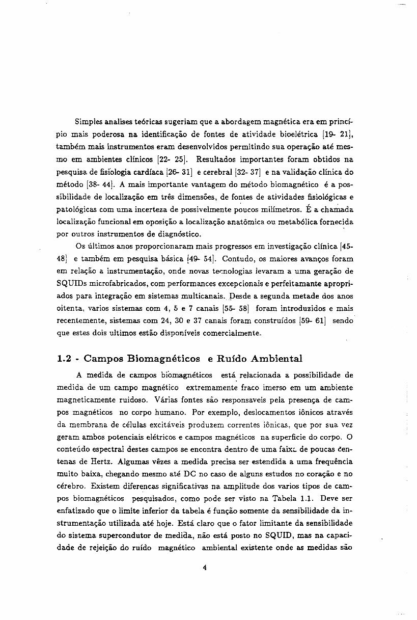
Simples analises teóricas sugeriam que a abordagem magnética era em princí

pio mais poderosa na identificação de fontes de atividade bioelétrica [19- 21],

também mais instrumentos eram desenvolvidos permitindo sua operação até mes

mo em ambientes clínicos [22- 25]. Resultados importantes foram obtidos na

pesquisa de fisiologia cardíaca [26- 31] e cerebral [32- 37] e na validação clínica do

método [38- 44]. A mais importante vantagem do método biomagnético é a pos

sibilidade de localização em três dimensões, de fontes de atividades fisiológicas e

patológicas com uma incerteza de possivelmente poucos milímetros. É a cha.IDa.da

localização funcional em oposição a localização anatômica ou metabólica forneci da

por outros instrumentos de diagnóstico.

Os últimos anos proporcionaram mais progressos em investigação clínica [45

48] e também em pesquisa básica [49- 54]. Contudo, os maiores avanços foram

em relação a instrumentação, onde novas ter.nologias levaram a uma geração de

SQUIDs microfabricados, com performances excepcionais e perfeitamante apropri

ados para integração em sistemas multicanais. _pesde a segunda metade dos anos

oitenta, varios sistemas com 4, 5 e 7 canais [55- 58] foram introduzidos e mais

recentemente, sistemas com 24, 30 e 37 canais foram construídos [59- 61] sendo

que estes dois ultimos estão disponíveis comercialmente.

1.2 - Campos Biomagnéticos e Ruído AmbientalA medida de campos biomagnéticos está relacionada a possibilidade de

medida de um campo magnético extremamente fraco imerso em um ambiente

magneticamente ruidoso. Várias fontes são responsaveis pela presença de cam

pos magnéticos no corpo humano. Por exemplo, deslocamentos iônicos através

da membrana de células excitáveis produzem correntes iônicas, que por sua vez

geram ambos potenciais elétricos e campos magnéticos na superficie do corpo. O

conteúdo espectral destes campos se encontra dentro de uma faix •..de poucas ~en

tenas de Hertz. Algumas vêzes a medida precisa ser estendida a uma frequência

muito baixa, chegando mesmo até DC no caso de alguns estudos no coração e no

cérebro. Existem diferencas significativas na amplitude dos varios tipos de cam

pos biomagnéticos pesquisados, como pode ser visto na Tabela 1.1. Deve ser

enfatizado que o limite inferior da tabela é função somente da sensibilidade da in

strumentação utilizada até hoje. Está claro que o fator limitante da sensibilidade

do sistema supercondutor de mediaa, não está posto no SQUID, mas na capaci

dade de rejeição do ruído magnético ambiental existente onde as medidas são

4

realizadas. Em primeiro lugar, temos o campo magnético terrestre com uma am

plitude de 50 ~Tesla. Este valor é 9 ordens de magnitude maior que o mais fraco

dos campos biomagnéticos. Portanto, vibrações do sensor no campo terrestre,

produzem grandes perturbações na medida. Em segundo, as micropulsações de

campos geomagnéticos: os chamados campos magnetotelúricos, põem uma depen

dencia da forma 1/! na amplitude do ruído impondo sérios problemas na parte de

baixa frequência no espectro da medida. Em último, os campos magnéticos asso

ciados com a presença de grandes massas metálicas, hélices, bombas, elevadores,

etc., geralmente existentes na proximidade do local de realização das medidas. A

amplitude deste último, chamado de ruído magnético urbano, está na faixa de

0.1 a 10 ~Tesla.

TABELA 1.1

CAMPOS

CAMPOSBIOELÉTRICOS

~VBIOMAGNÉTICOS pTBANDA Hz

Eletrocardiograma

1000Magnetocardiograma500.05 - 100Eletrocard. Fetal

5 - 50Magnetocard. Fetal1-100.05 - 100

Eletroencefalograma50Magnetoencefalograma10.5 - 30

Potenciais Evocados10Campos Evocados 0.1DC - 50

Eletromiograma1000Magnetomiograma 10DC - 2000

EletrO-oculograma1000MagnetO-oculograma10DC

Tabela 1.1 - Intensidade de campos bioelétricos e biomagnéticos.

1.3 - SQUIDs e Discriminação Espacial

O detector de campo magnético mais simples é uma bobina. Um campo

magnético variante no tempo passando através da bobina gera uma corrente que

pode ser detectada e amplificada (Lei de Faraday). A limitação da utilização da

bobina de indução é o ruído associado à resistência da própria bobina. Uma analise

simples pode mostrar que o campo mínimo detectavel é inversamente proporcional

a frequência do sinal [62]. Como em biomagnetismo o interesse está em medidas

em baixa frequência (0-100 Hz), a aplicação de bobinas de indução à temperatura

ambiente é limitada. A utilização de magnetômetros ftuzgate ou de magnetômetros

5

baseados no efeito Hall também tem sua aplicação limitada devido a sua baixa

sensibilidade para esta faixa de frequência.

A relativa baixa sensibilidade em baixas frequências dos magnetômetros con

vencionais, pode então ser melhorada através de utilização de circuitos supercon

dutores. A bobina de detecção neste caso fica intrinsecamente livre de ruído e um-.Superconducting QUantum Interference Device (SQUID) [63- 64] pode ser usado

como amplificador. Este dispositivo é uma aplicação do efeito Josephson [65- 66]

e requer a utilização de técnicas criogênicas. O possível aumento de problemas

técnicos dada a utilização de hélio líquido, é largamente justificado pelo ganho desensibilidade.

OEWAR

IQUID

ELETtGUlD

Fig. 1.1 - Desenho esquemátic..:>de um sistema para medidas biomagnéticas.

A figura 1.1 mostra esquematicamente o sistema criogênico contido em um

dewar de fibra de vidro com superisolamento [67]. O reservatório de hélio líquido,

necessário para manter o circuito supercondutor a uma temperatura de 4.20

Kelvin, usualmente mantém o sistema frio por alguns dias. O campo magnético

que passa através da bobina de detecção é sentido pelo SQUrD através da corrente

supercondutora existente no circuito composto pela bobina de detecção e por uma

bobina interna ao SQUID. Com a bobina interna fortemente acoplada, esta super-

6 -

corrente impõe um fluxo magnético ao SQUID, que com a ajuda de uma eletrônica,

transforma este fluxo em tensão. A tensão de saida é linearmente proporcional ao

fluxo de entrada por varias décadas de frequência. Os SQUIDs não são dispositivos

passivos, eles precisam ser polarizados ou por rádio frequência (rf-SQUIDs) [68

69] ou por corrente contínua (dc-SQUIDs) [70- 71]. Os rf-SQUIDs são bastante

confiáveis, relativamente simples de serem construídos e estão disponíveis comer

cialmente desde meados da década de setenta. Os dc-SQUIDs, embora disponíveis

comercialmente há alguns anos, ainda são objetos de estudo [72- 73]. A princípio

os dc-SQUIDs podem ser mais sensíveis que os rf-SQUIDs por várias ordens de

magnitúde.

Como já foi dito, a medida de campos biomagnéticos só é possível através

da redução do ruído magnético presente no ambiente onde as medidas são real~

zadas. Esta redução geralmente é feita de duas formas: 1- utilização de câmaras

magneticamente blindadas [74- 76] de forma a isolar o paciente e o instrumento

de medida do ruído ambiental e 2- utilização de sensores que acoplados ao SQUID

sejam capazes de discriminar fontes distantes (ruído) em favor de fontes próximas

ao sensor (sinal biomagnético). A primeira técnica, do ponto de vista de um

laboratório urbano ou de um hospital, não é muito conveniente, devido ao seu

alto custo de fabricação e ao desconforto para o oaciente devido ao pouco espaço

usualmente disponível em seu interior. A segunda técnica é conhecida como dis

criminação espacial e os sensores como gradiômetros já que medem diferenças

ou derivadas do campo no espaço. Os gradiômetros podem ser axiais, confec

cionados com fio supercondutor enrolado em volta de um mandril cilíndrico, ou

podem ser planares, integrados junto com dc-SQUIDs em um substrato de silício.

A discriminação espacial será estudada a partir do próximo capítulo.

7

2 GRADIÔMETROS AXIAIS

Neste capítulo será abordado o princípio básico de funcionamento dos gradiô

metros axiais, seu projeto, sua construção, medidas de performance e calibração.

Detalhes adicionais podem ser encontrados na publicação [1].

2.1 - Caracterização Usando a Expansão de Taylor

Considere que uma fonte pode ser modelada por um dipolo magnético m e

produz um campo B (r) dado por [77]:

B(r) == J.Lo [3(r.m)r _ m]471" r r3'(2.1)

o fluxo devido a este dipolo em uma espira de uma bobina sensora pode serexpresso como:

i B(r)dA,(2.2)

onde dA é um elemento de área e a integral se estende sobre toda área da bobina.

Substituindo Eq. (2.1) na Eq. (2.2) e efetuando a integração, temos que o fluxodevido ao dipolo localizado no eixo da espira e a uma distancia d é:

(2.3)

onde R é o raio da bobina.

Suponha agora que exista uma outra espira sensora no mesmo eixo a uma

distancia b da primeira, portanto a uma distancia b + d do dipolo. O fluxo atravésdela será dado por:

q" = I'~I~I[1+ (d; b),r (2.4)

Se as espiras forem conectadas em série e enroladas em sentidos opostos, cons

tituindo assim um gradiômetro de primeira ordem (Fig. 2.1), o fluxo resultanteserá dado por:

(2.5)

8

6---•

b

-I

I II I'----J

R

Fig. 2.1 - Desenho esquemático de um gradiômetro de primeira ordem.

Temos então que para fontes distantes <Pt tende a zero (d ~ b), ao passo

que para fontes próximas existirá um <Pt não nulo. Este é o princípio básico de

funcionamento dos gradiômetros: drástica atenuação de campos provenientes de

fontes distantes em relação a campos provenientes de fontes próximas.

De uma forma mais geral, a equação que descreve o fluxo magnético induzido

em um conjunto de (N + 1) bobinas conectadas em série, cada uma constituida

por n, espiras de mesma área A é (Fig. 2.2):

(2.6)

onde Zi é a distância da bobina i à origem Zo, Bz (z) é a componente vertical,

perpendicular ao plano da bobinas, do campo magnético B(z) e f(t) a dependência

temporal deste campo.

Expandindo Bz (z) em série de Taylor em torno da origem Zo temos:

00 B(a)( )B ( ) - ~ z Zo (_ )a"z -L- , z Zo ,a.

a=O(2.7)

onde B~a) (Zo) é a derivada de ordem Q de B" (z) no ponto Zo. Substituindo a

equação acima na Eq. (2.6) teremos:

4>(t) = A [~t:B!·~~Z,)(z, - z,). ] I(t).

9

(2.8)

ftN ct:>-----. ----•

ft3 ct:>------". ~ - - - - - - ~ - - -

ftl b---:---JI Ib 2no C>--- ~I - _F_- -1- __

Fig. 2.2 - Desenho esquemático de um conjunto de (N+1) bobinas

Chamando de bi (linha de base) as distâncias Zi - Zo e explicitando a expansão em

Zo = O teremos:

b2

4>(t) = A{ no Bz (O) + ndBz (O) + B~ 1) (0)b1 + Bi2) (O) 2. + ...2

+ n2[Bz (O) + B;l) (0)b2 + B;2) (O) b; + ...2

+ ... } f(t), (2.9)

ou matricialmente:

4>(t) = (A

onde:

O

f(t), (2.10)

a = O, ... , N - 1. (2.11)

A matriz diagonal acima representa o efeito do conjunto de bobinas do gradiômetro

sobre o campo e suas derivadas na origem.

A distinção fundamental entre a dependência espacial de uma fonte distante

e de uma fonte próxima, é a importância relativa do campo e de suas derivadas

num determinado ponto do espaço. No caso da fonte distante, os termos na Eq.

(2.10) que envolvem o campo e as primeiras derivadas são predominantes diante

do demais. No caso da fonte próxima isto não ocorre.

Para exemplificar, suponhamos que três fontes com uma dependência espacial

dipolar ~ e com constantes de proporcionalidade K1, K2 e Ks estejam respecti-r

vamente a 100, 10 e 1 unidades de comprimento do ponto de medida Zo. Mesmo

10-

quando K1 ~ K2 ~ K3 as derivadas de ordens mais elevadas da fontes distantes

tendem a zero, ao passo que as derivadas da fonte próxima tendem a divergir. Isto

pode ser observado na Tabela 2.1, para K1 = 108, K2 = Ia" e K3 = 1.

TABELA 2.1

(K,r)

campoIa derivada2a derivada3a derivada

(108, 100)

10030.120.006

(10", 10)

1031.20.6

(1,1)

131260

Tabela 2.1- Derivadas espacias de uma fonte com dependência dipolar ~ para váriosrvalores de K e r.

Portanto, se conseguirmos anular os primeiros termos da matriz diagonal da

Eq. (2.10), estaremos anulando a contribuição dos sinais provenientes de fontes

distantes. Deve ser mencionado que o fato das derivadas de uma fonte próxima

divergirem, significa que a expansão de Taylor não é válida para este caso.

Para projetar um gradiômetro de ordem N, assumindo a área A constante,

as primeiras (N-l) equações de (2.11) devem ser zeradas de forma a rejeitar o

ruído. Por exemplo, um gradiômetro de primeira ordem anula a componente

espacialmente constante do campo, portanto Uo = O. Um gradiômetro de segunda

ordem anula a componente constante e a primeira derivada, Uo = U1 = Oe assim

sucessivamente. Procedendo desta forma temos que o projeto do gradiômetro deve

obedecer ao seguinte sistema de equações:

a=O,I, ... ,N-1. (2.12)

o gradiômetro ficará definido ao se conhecer o número de voltas de cada

bobina e a distância entre elas, ou seja, o conjunto {ni, bi j i = O,... , N}. Por

inspeção visual, podemos notar que o sistema (2.12) tem N equações e 2N + 1

incógnitas. Portanto, N + 1 incógnitas devem ser transformadas em parâmetros

para tornar sua solução possível. Dependendo de quais variáveis forem escolhidas,

serão gerados dois tipos de soluções. Por exemplo, suponha que os N bi IS (b1 , b2 =

11

2b1, ••• , bN = Nbd e um n, (no) sejam escolhidos. Neste caso a solução para o

sistema tem a forma da fórmula binomial de Newton [62] :

n, = no(-1)'-1 (. N )~- 1 ' i = 1,... ,N - 1. (2.13)

Esta solução leva ao projeto de gradiômetros convencionais. Por exemplo, um

gradiômetro de primeira ordem, como já foi mencionado, será especificado por

no = 1, n1 = -1 e b1 = b. Um de segunda ordem por no = 1, 711= -2, n2 = 1,

b1 = b e b2 = 2b, e assim sucessivamente.

No entanto, um tratamento mais geral, nunca fora abordado na literatura.

Se os (N + 1) n, '5, forem escolhidos de forma a resolver a primeira equação de

(2.12), então mais um incógnita precisa ser escolhida. Suponha que o comprimento

total do gradiômetro bN seja a incógnita escolhida. Neste caso teremos a escolha

mais geral possível, pois levará às soluções (2.13) e outras onde os b, '5 não serão

múltiplos uns dos outros (vide anexo 1). Como exemplo, pode ser citado um

gradiômetro de terceira ordem co,m no = 2, n1 = -3, n2 = 2, n3 = -1, b1 = O.15b,

b2 = O.73b e b3 = b.

Adotando-se esta última solucão ou a primeira, é necessário algum critério

para a escolha de bN e dos n, '5• O gradiômetro é o produto de um modelo de

projeto (expansão de Taylor) que só é possível se a série representada pela Eq.

(2.8) convergir. Isto é, se a expansão for válida para a dependência espacial do

sinal em questão. Isto significa dizer que a dependência espacial do sinal próximo

deve divergir, de forma que o conjunto de bobinas da Fig. (2.2) não funcione como

um gradiômetro para este sinal. Vamos exemplificar projetando um gradiômetro

de segunda ordem. O sistema a ser resolvido é o seguinte:

no + n1 + n2 = O

(2.14)

Escolhendo os n, '5 de forma a satisfazer a primeira equação de (2.14) e de forma

a não gerar uma linha de base negativa, (n2 deve ter sinal contrário a n1), temos:

(2.15)

(2.16)

Resta agora a escolha de b2• Para um gradiômetro de segunda ordem, podemos

exprimir matematicamente a divergência da Eq. (2.8) como:

}~~ IT~+l I > 1,a

12

onde,

(2.17)

e B% (Zo) é o campo do sinal próximo na primeira bobina. A expressão geral para

B~a) para campos da forma K / zm pode ser escrita como:

(2.18)

onde z é a distância da fonte a origem, escolhida na primeira bolJina. Substituindo

as Eqs. (2.15) e (2.18) na Eq. (2.16) e efetuando o limite, temos que Ib21 > Izl.

Portanto, o comprimento total do gradiômetro deve ser maior que a distância

da fonte de sinal biomagnética a primeira bobina do gradiômetro. Com relação

a escolha apropriada dos ni 15, outras limitações de natureza prática devem ser

levadas em consideração.

2.2 - Aspectos Práticos na Construção de Gradiômetros

Como já foi mencionado, a utilização do gradiômetro se faz juntamente

com o SQUID. Este acoplamento é realizado de forma indutiva, utilizando um

transformador de fluxo onde o secundário é colocado no interior do SQUID e o

gradiô.metro funciona como primário deste transformador [78]. Como se trata deum circuito supercondutor, para um fluxo externo tPe aplicado ao gradiômetro,temos:

tPe + (Lg + L. )i. = O, (2.19)

onde Lg e L. são respectivamente as indutâncias do gradiômetro e do secundário

no interior do SQUID, e i, é a corrente-su~ ~rcondutora gerada. Como entre L. e

o SQUID existe uma indutância mútua dada por M., existirá portanto, um fluxo

tP, induzido no SQUID igual a :

(2.20)

Para rf-SQUIDs comerciais, M, e L, são parâmetros fixos, assim a transferência

de fluxo ao SQUID é função da indutância do gradiômetro. Para maximizar a

transferência de energia L. e Lg devem ter aproximadamente o mesmo valor. Para

13

o caso particular dos rf-SQUIDs da Biomagnetic Technologies, Inc. L, é igual a

2 J.LH. A indutância de uma bobina circular pode ser expressa como:

8RL = n2 0.0411" R (ln- - 2) J.LH,

. P(2.21)

onde, n é o número de voltas da bobina, R é o raio da bobina e p o raio do fio que

. compõe a bobina. Portanto, Lg depende do número de bobinas, número de voltas

de cada espira da bobina e da sua área. Assim, o valor de Lg deve ser tal que:

N 8RLn~ 0.0411" R (ln- - 2) ~ 2 J.LH.i= o p

(2.22)

Os gradiômetros são construídos enrolando-se fio de nióbio puro ou nióbio

titânio, com aproximadamente 0.1 mm de diâmetro, sobre um mandril cilíndrico

de CELERON ou MACORTM, após a confecção em locais apropriados de sulcos

aonde será colocado o fio. O fio é fixado ao mandril com cola tipo superbonder.

Note que a construção real do gradiômetro projetado, obviamente não vai atender

as equações do sistema (2.12), já que é função do processo de contrução utilizado,

e a precisão usualmente alcançada é de decímos de milímetro. Isto acarretará

que, para um gradiômetro de segunda ordem, a rejeição ao campo não será igual

a zero e a rejeição a derivada do campo também não será nula. O chamado

. desbalanceamento [79] de ordem zero corresponde a não rejeição total do campo e

o desbalanceamento de primeira ordem corresponde a não rejeição da derivada do

campo. Neste caso, devemos escrever o sistema (2.14) levando em consideração asdiferentes áreas de cada bobina:

noAo + nlAI + n2A2 :::::O

nl AI bl + n2 A2 b2 :::::O. (2.23)

Podemos então, representar um gradiômetro real como um gradiômetro ideal mais

o desbalanceamento, que é função da ordem do gradiômetro. Um gradiômetro

de segunda ordem real pode ser representado como a soma de um gradiômetro

ideal mais uma pequena espira que corresponde a detecçáo de parte do campo

e um pequeno gradiômetro de primeira ordem que corresponde à detecção de

parte do gradiente do campo. Note, queeste desbalanceamento está relacionado a

resposta axial, ou seja, na direcao z do gradiômetro. Além disso, existe também o

14 -

desbalanceamento relacionado ao não perfeito alinhamento dos planos das bobinas

isto é, nas direcões x e y.

Para compensação dos desbalanceamentos, várias técnicas podem ser uti

lizadas [9,22]. A mais simples e bastante confiável consiste no deslocamento dentro

do gradiômetro de peças supecondutoras [80]. Como, devido ao efeito Meissner, no

interior das pequenas peças o campo é nulo, sua aproximação às espiras terá o efeito

de área negativa compensanq,o assim os erros no processo de construção. Pode ser

observado no sistema (2.23) que atuando nas áreas estaremos afetando' tanto o

desbalanceamento de ordem zero como o de primeira ordem. Para a precisão

usualmente alcançada na confecção dos gradiômetros com diâmetros variando en

tre 1.5 e 3 em, são utilizados discos de chumbo entre 004 e 1 em de diâmetro, para

o balanceamento axial. Para o balanceamento em relação aos planos das bobi

nas são utilisados 2 pequenos retângulos posicionados perpendiculan;nente um ao

outro, com os lados variando entre 0.3 x 0.6 em e 0.7 x 1 em.

2.3 - Testes de Performance e Calibração

Foram contruídos, testados e comparados entre si, vários gradiômetros de

primeira, segunda e terceira ordens. Estes testes consistiram na avaliação da

relação sinal-ruído do campo magnético gerado pelo coração humano. Pode ser

constatado que cada ambiente terá o seu gradiômetro ótimo, já que o seu projeto

é sempre uma solução de compromisso entre sinal e ruído, e o ruído será sempre

característico do ambiente de medida. Para o caso de gradiômetros não balancea

dos, um gradiômetro de terceira ordem foi, para o nosso caso, e a escolha mais

conveniente, como pode ser constatado na Fig. 2.3.

Como a leitura na saida do SQUID é feita em Volts devemos transformá

ia para a unidade de campo magnético Tesla, já que a transferência de fluxo do

gradiômetro ao SQUID depende da indutância do gradiômetro usado. Esta trans

formação pode ser feita através das seguintes calibrações: aplica-se ao gradiômetro

um campo gerado por um dipolo magnético. O dipolo é realizado através de

um pequena bobina circular com diâ.metro bem menor do que o diâmetro D do

gradiômetro, colocada axialmente à um distância z não inferior a 10 vezes o raio

do gradiômetro. Mede-se a corrente aplicada a bobina e calcula-se o fluxo 4>(z)

que a bobina gera no gradiômetro:

4>(z) = J1.o; (1 + ~: t 3/2. - (2.24)

15

o

b

, •• ", •• " •••• 1 •••• '.' •• "," ,., "'" ,.\ ""I 2.?p'T,,,,,, "" ,.", .•",,"','" ',', ••., '"'''''' ,.",

Ifn"''''I''''I'II'~lftll''IfI'tt''''''I''''II35PT ~I •.• I •••• 11I1I111111'1111111111III'lflI11.45••••• 111111"111'''1

Fig. 2.3 - Comparação de um sinal magnetocardiográfico obtido por um gradiômetro de

terceira ordem (a) e um gradiômetro de segunda ordem (b) sob as mesmas condições .

Observando a tensão na saída do SQUID e dividindo o fluxo no gradiômetro pela

área efetiva da primeira bobina, obteremos a relação teslajvolt.

Um outro método que também pode ser utilizado, consiste na colocação de

uma bobina em volta da cauda do dewar criogênico que contém o sistema. Move-se

a bobina ao longo do gradiômetro, até a saida do SQUID apresentar uma tensão

máxima. Da geometria do gradiômetro e da bobina, e das suas posições relativas,

a indutância mútua entre os dois pode ser calculada [81]. Multiplicando-s~ a cor

rente na bobina pela indutância mútua, tem-se o fluxo aplicado ao gradiômetro.

Dividindo o fluxo no gradiômetro pela área efetiva da primeira bobina, obtere

mos a relação teslajvolt. Na Tabela 2.2 podem ser observados as calibrações C

teslajvolt medidas para diversos gradic'metros construídos no laboratório.

O método pelo qual se avalia a rejeição de um gradiômetro à componente

espacialmente constante do ruído, consiste na geração de um campo constante no

espaço, em uma frequência temporal conhecida, na região do gradiômetro. As

peças supercondutoras são então deslocadas no seu interior, de forma a anular o

campo aplicado. Foram contruídas no laboratório, dois tipos de bobinas para a

geração deste campo uniforme. A primeira consiste em um par de Helmholtz com

aproximadamente 1 m de diâmetro.- A segunda consiste em um conjunto de quatro

bobinas quadradas [82] formando aproximadamente um cubo de 1 m de lado.

16

Fig. 2.4 - Espectro de frequência de um gradiômetro segunda ordem balanceado.

TABELA 2.2

Ordem

ni I sbi I SD(em)L(p.H) C

segunda

1,-2,10,5,101.50.46.5 x 10-8

segunda

3,-6,30,5,101.51.52.9 x 10-8

segunda

4,-8,40,4,81.52.02.5 x 10-8

segunda

1,-2,10,5,103.00.82.3 x 10-8

terceira2,-3,2,-10,3.1,14.6,20 3.01.91.6 x 10-8

Tabela 2.2 - Calibrações medidas de diversos gradiômetros construídos. As cali

brações estão em ordem crescente de sensibilidade.

A uniformidade do campo gerado pelo segundo conjunto de bobinas é melhor que10- 4 dentro de um volume de 10 x 10 x 10 em no centro do cubo.

Na Fig. 2.4 pode ser observado o espectro de ruído de um gradiômetro de

segunda ordem balanceado. A linha de base do spectro é 50 fT /.JIj";.

17

-- --"---,

Definindo o desbalanceamento como o fator de rejeição do gradiômetro ao

campo aplicado, temos que aplicando um campo em três direções perpendiculares

e sabendo sua intensidade, poderemos obter o valor da rejeição. O valor 'nor

malmente conseguido está na faixa de -60dB a -40dB, para gradiômetros sem

balanceamento. Balanceando-se o g~adiômetro este fator pode chegar a -IOOdE.·

Um método prático de se certificar que o gradiômetro está bem balanceado é

o seguinte: além da eliminação dos picos de frequência indesejáveis no seu espectro,

deve ser comparado o valor da linha de base em freqüências mais altas, por exemplo

400-500 Hz com o valor da linha de base em baixas frequências, por exemplo 0-10

Hz. Se estes valores forem semelhantes o gradiômetro está bem balanceado.

18 -

3 FILTROS ESPACIAIS

Neste capítulo um novo modelo para gradiômetros, baseado em conceitos de

filtragem digital, é introduzido. Novos tipos de projeto são propostos, a função

de transferência experimental é medida e também é rediscutida a calibração do

sistema. Nas p~blicações [2], [3], [4], [5], [10] e [12] detalhes adicionais podem serencontrados. Vale ressaltar que até então a descrição de um gradiômetro usado

por determinado laboratorio era feita com base em suas características geométricas

(diâmetro, comprimento, número de bobinas etc.)

3.1 - Caracterização Usando a Transformada de Fourier

A relação entre um gradiômetro e um filtro espacial pode começar a ser

entendida se utilizarmos o chamado princípio da reciprocidade [83- 85]. Note que

o campo produzido por uma espira quando percorrida por um corrente I é:

(3.1)

onde d é a distancia ao ponto de medida e R o raio da bobina. O chamado campo

recíproco dado pela Eq. (3.1) tem a mesma dependência em R e em d que o fluxo

dado pela Eq. (2.3). Isto significa que, o fluxo induzido em uma espira por um

dipolo magnético colocado em seu eixo, cai com a distancia da mesma forma que

o campo axial que ela produz quando percorrida por uma corrente I. Utilizando

esta reciprocidade, está esquematizado na Fig. 3.1 o fluxo induzido por uma fonte

dipolar, em uma única espira e em um gradiômetro de primeira ordem, em funçãoda distância.

Como pode ser observado, a sensibilidade do gradiômetro à fontes mais

distantes é muito menor do que a de uma bobina. Podemos então, associar o

gradiômetro a um filtro passa-perto. Este princípio poderia ser bastante útil

para se comparar o desempenho dos diversos tipos de gradiômetros. Contudo, o

princípio da reciprocidade só é valido para fontes que possam ser modeladas através

de dipolos magnéticos, que é o caso do ruído. No caso do sinal biomagnético, por

razões físicas, as fontes são modeladas por dipolos de corrente [86- 87], que tem

uma dependência espacial diferente. Portanto não podemos utilizar o princípio

da reciprocidade para avaliar a discriminação espacial efetuada por determinado

19

oo~N~«2a:O 1.0zOON::lO 10-3Z

OX::l~~

GRADIÔMETRO

10 100

DISTÂNCIA(U.A)

ESPIRA

1000

Fig. 3.1 - Sensibilidade de um bobina e de um gradiômetro de primeira ordem a uma fonte

dipolar em função da distância.

gradiômetro. Este incoveniente pode ser superado se pensarmos no gradiômetro

com um filtro não no domínio das distâncias mas no domínio das frequências

espaciais (vide anexo 2). Além disso, o gradiômetro será visto como um dispositivo

digital, que atua em pontos discretos no espaco (vide anexo 3)

O gradiômetro é um dispositivo que amostra sinal e ruído variantes no

tempo, em pontos discretos no espaço, que correspondem às posições das bobinas.

Portanto, trata-se de um amostrador espacial. O período de amostragem espacial

é dado pela distância mínima entre as bobinas ),•. Além disso, é feita a soma

ponderada dos sinais amostrados em cada instante de tempo. Os fatores de pon

deração dependem da área de cada bobina. Portanto, o gradiômetro é um filtro

espacial não recursivo. Isto pode ser melhor compreendido através dos seguintes

argumentos (vide anexo 5): os elementos básicos de ULJ. filtro digital são o unit

delay o somador e o multiplicador. Portanto, filtros digitais são coleções de inter

conexões dos três elementos acima [88]. Podemos encontrar no gradiômetro todos

os elementos corrrespondentes aos do filtro digital. O período de amostragem ),.

corresponde ao unit delay. O fato das bobinas estarem enroladas em série cor

responde ao somador. Finalmente, o fato de medirmos o fluxo, que em primeira

aproximação é o campo multiplicado pela área de cada bobina, corresponde ao mul

tiplicador. Parece então apropriãda, a utilização de um formalismo matemático

digital para descrever o sensor gradiométrico.

20

Dentro deste formalismo, a saída de um filtro não recursivo também chamado

moving average filter pode ser expressa como [89]:

00

Ym

,= - 00

(3.2)

Este procedimento define um novo conjunto de numeros Ym provenientes do con

junto Xm, que corresponde a entrada do filtro amostrada em intervalos constantes.

Os fatores de ponderação h, determinarão a característica do filtro. A grande

vantagem da utilização deste formalismo está no fato de podermos caracterizar o

gradiômetro e portanto a sua atuação, independente de qualquer suposição prévia

sobre o comportamento espacial de sinal e ruído (vide anexo 3). Esta caracte

rização se dará através de uma função de transferência no domínio das frequências

espaciais.

Para o caso do gradiômetro, assumimos que as linhas de base b, podem ser

expressas como múltiplos do período de amostragem À;, b, = p, À., onde p, são

valores inteirc,s. O sinal detectado pelo gradiômetro na posição Zm, assumindoum numero infinito de bobinas é :

00

(3.3)i= - oc

ou considerando a natureza digital do sistema,

00

4Jm = A L n,Em_"i=-co

(3.4)

onde A é a área do gradiômetro, ni é o número de voltas de cada bobina e Em _ ,

é O valor do campo magnético na i-ési!lla bobina em algum instante do tempo e

numa dada posição m.

Se aplicarmos a transformada discreta de Fourier (DFT) na Eq. (3.4) tere-mos:

00

i= - 00

(3.5)

00 00 00

(3.6)m=-oo m=-oo '=-00

21

Invertendo a ordem dos somatórios e após algumas manipulações na Eq. (3.6)obtemos:

oc

m=-cx> i= - 00

oc

m=-ex>(3.7)

~(k) = AH(k) B(k), (3.8)

onde ~ (k) e B (k) são respect ivamente a DFT da saída e da entrada do filtro

(gradiômetro) e H(k) é a sua função de transferência. Portanto a função dê:trans

ferência espacial de um gradiômetro é a DFT do conjunto representado pelo

número de voltas de cada bobina. Como no gradiômetro real temos somente

(N + 1) espiras,N

H(k) = A L nie-jiU ••i=O

(3.9)

o espectro de Fourier de um sinal distante só tem componentes de baixas

frequências espaciais, enquanto que um sinal próximo tem componentes de baixas

e altas frequências (vide anexo 3). Portanto, a discriminação espacial é realizada

porque o gradiômetro atua como um filtro passa-alta frequência espacial (Fig.

3.2).

4.0 r •••_/\H(K)I I I I /

., /II I /

UJ 1 .. I 1/~ :3.0 I!!!., /O . Ia... i.. ••••.•.••• s /

~ I~ 3,d/UJ 2.0 / ..••..••.-'O I 2nd""::::l I ",-I- / /::::i 1 //~ 1 /::E / / 1st<[ 1.0 / ////

~",;,.--.",

.~",.OO .5

K/K.

Fig. 3.2 - Funções de transferência de gradiômetros de primeira. segunda e terceira ordens.

22 -

3.2 - Projeto de Filtros Espaciais

Será visto como projetar novas e tradicionais configurações de gradiômetros

utilizando técnicas de filtragem digital. As configurações tradicionais aparecem se

for utilizado um procedimento que parte de projetos de filtros analógicos para se

chegar às realizações digitais. Novas configurações aparecerão se forem utilizadas

diretamente técnicas de projeto de filtros digitais.

As configurações tradicionais [79] são obtidas se a seguinte técnica de projeto

for utilizada para projetar filtros passa-alta. A condição que garante a eficácia de

um filtro passa-alta smooth é:

8a8ka H(O) = O

, a:: = O, ... , N - 1 (3.10)

onde N é a ordem do filtro. A Eq. (3.10) mostra que se as sucessivas derivadas

da função de transferência na origem (k = O) são nulas, sua banda de rejeição se

torna mais plana. Esta condição no formalismo de filtragem, é idêntica a condição

(2.12) obtida no formalismo de Taylor (vide anexo 2).

Como já foi mencionado, um método de projetar um filtro digital é achar a

função de transferência apropriada, H (8), no domínio de Laplace usando a teoria

clássica de filtragem. O projeto analógico é então transformado em uma realização

digital [90]. Um possfvel projeto que tem a banda passante da função de trans

ferência plana é conhecido como Butterworth. Contudo a condição expressa na

Eq. (3.10) requer a banda de rejeição plana. Apesar disso, o polinômio de But

terworth, Hb(8), ainda pode ser utilizado para projetar a função de transferência

desejada, Ha (8) da seguinte forma:

(3.11)

Podemos escrever Hb (8) como:

(3.12)

substituindo a Eq. (3.11) em (3.10) temos,

(3.13)

Este Ha (s) assegura uma função de transferência com a banda de rejeição plana,

já que obedece a condição expressa na Eq. (3.10).

23

A realização (3.13) do gradiômetro pode ser feita utilizando alguma das

transformações do domínio de Laplace para o domínio digital. Isto consiste em

substituir a equação diferencial relacionada com Hg (8) por uma equação diferença.

Isto é feito realizando a seguinte substituição de variáveis (vide anexo 5):

1 - 18 = - Z , (3.14)

onde z é a variável no domínio digital (z = eikÀ'). Portanto, H (z) pode ser escritaCJmo:

Por exemplo pa,ra N = 1 teremos:

H(z) = 1- z- 1 ,

para N = 2,

H(z) = 1-2z-1 +Z-2,

(3.15)

(3.16)

(3.17)

e assim sucessivamente. Estas expressões dos filtros não recursivos, tem embutidas

todos os elementos necessários à construção do gradiômetro. O primeiro elemento

da Eq. (3.17) representa a primeira bobina com 1 volta. O segundo, uma bobina

com 2 voltas em sentido oposto à um distancia >., da primeira. Finalmente o ter

ceiro, uma bobina com 1 volta no mesmo sentido da primeira e a 2 >'. da primeira.

Assim, as mesmas configurações utilizando a Eq. (2.13) são obtidas com este novo

formalismo, só que agora de uma forma mais geral e com uma justificativa lógica.

Se utilizarmos agora uma técnica de projeto que use diretamente conceitos

de filtragem digital, obteremos novos tipos de filtros espaciais passa-alta que não

chamaremos mais de gradiômetros, mas de diferenciadores. A diferença entre um

gradiômetro e um diferenciador é que o gradiômetro somente funciona com um

diferenciador para sinais de baixa frequência espacial (vide anexo 5).

Como já foi visto, a expressão geral para um filtro não recursivo é dada

pela Eq. (3.2), onde os coeficientes h, devem ser considerados como as áreas das

bobinas do sensor. Estes coeficientes podem ser obtidos diretamente, calculando-se

a transformada de Fourier inversa de H (k ):

(3.18)

24

o diferenciador tem como função de transferência H(k) = Jk. No domínio digitalteremos:

H(k) = Jk, . para - 7r/>". < k < 7r/>.. •. (3.19)

Substituindo a Eq. (3.19) na Eq. (3.18), efetuando a integração , e truncando o

resultado para um numero N finito de bobinas, teremos:

para i = 1, ... , N (3.20)

e para i = O, h, = O. A truncagem desta sequência vai resultar em um função

de transferência com uma característica oscilatória. Entretanto, os ripples podem

ser virtualmente eliminados ao se utilizar uma técnica de janelamento diferente.

Repare que ao trucarmos a sequência (3.20) estàmos usando uma janela que tem

o valor 1 no intervalo i = 1, ... , N e zero no resto. Se ao invés do fator 1, usarmos

um janela de Hamming dada pela expressão :

~7r

W, = 0.54 + 0.56 cos( N)' para i = O... N , (3.21)

e multiplicarmos cada termo de (3.20) pelos tenÍlos correspondentes em (3.21),

obteremos a função de transferência (linha contínua) mostrada na Fig. 3.3. A

linha pontilhada na mesma figura é a de um diferenciador ideal. Como pode ser

observado, o resultado é bastante satisfatório. Também esta mostrada na Fig. 3.3

a característica (traço-ponto) de um gradiômetro de primeira ordem. Note que

para baixas frequências a função de transferência de um gradiômetro é igual a

de um diferenciador. No inset da Fig. 3.3 estão desenhados esquematicamente

um gradiômetro de primeira ordem no = 1, nl = -1, b1 = b e um diferenciador

no = 0.25, n1 = -0.5, n2 = 1, n3 = -1, n" = 0.5, n5 = -0.25, b1 = b, b2 = 2b,

b3 = 3b, b" = 4b ( b5 = 5b.

Pelo menos teoricamente, os diferenciadores são filtros com desempenho su

perior aos gradiômetros. Isto porque, para baixas frequências, o desempenho é o

mesmo, e para altas frequências o ganho é maior.

3.3 - Medida da Função de Transferência

Após estas considerações teóricas, onde se obteve a função de transferência de

um gradiômetro, ou de forma mais geral, de um filtro espacial, parece interessante

25

o

1:-." 1I

1=- mI - ==

05 1.0

Fig. 3.3 - Funções de transferência de um diferenciador ideal. um diferenciador com um

número de bobinas finito e um gradiômetro de primeira ordem.

que essa função de transferência, uma vez construí do o filtro, possa ser medida.

Isto pode ser realizado, aplicando-se um sinal conhecido ao filtro, e medindo-se

a sua resposta como função de uma coordenada espacial (vide anexo 4). Como

mostrado em (3.8), se dividirmos a transfo'rmada de Fourier do sinal de saída

~ e:z: p (k) medido, pela transfo:mada de Fourier do sinal de entrada 8 (k), estaremos

por definição, ol?tendo a função de transferência real H~:z:p(k) do filtro:

He:z:p(k) = ~e:z:p(k)_"a" • (3.22)

A magnitude de Hr (k) poderá ser então comparada com a magnitude da função de

transferência teórica, obtida através da DFT dos coeficientes do filtro (gradiôme

tro).

A saída do gradiômetro é a soma dos sinais detectados por todas as bobinas.

A entrada será considerada como o sinal detectado somente pela primeira bobina

do gradiôrnetro. O sinal de entrada utilizado, será a distribuição espacial do campo

magnético gerado por uma bobina. As dimensões desta bobina serão escolhidas

conforme os seguintes critérios. O raio da b ..}binadeve ser grande o suficiente, de

forma a permitir o seu deslocamento através do dewar (Fig., 1.1). Este deslocamento é necessario para termos um valor para a saída em vários pontos no espaço.

Contudo, o raio deve ser pequeno o suficiente para gerar um distribuição espacial

apropriada para a transformada de Fourier, de forma a evitar o efeito conhecido

como aliasing. Uma simulação em computador foi feita e um bom compromisso

foi alcançado com um raio de cerca de 15 cm.

Uma estrutura foi construída delorma fixar a bobina em relação ao plano

x - y, permitindo somente movimentos ao longo do eixo do gradiômetro z. O

26 -

dewar contendo o gradiômetro, é colocado em um suporte concêntrico em relacao

a bobina. A bobina então é deslocada de uma posição 1 m abaixo do centro do

gradiômetro à mesma posição acima do centro. A bobina é deslocada em passos

de 2.5 cm quando longe, e 1 cm quando perto do gradiômetro. Uma corrente de

baixa frequência é aplicada à bobina, e o resultado na saída do SQUID é lido com

ajuda de um amplificador lock-in. Foram obtidas várias funções de transferências,

como exemplo, pode ser visto na Fig. 3.4 as funções de transferências teórica e

real de um gradiômetro de segunda ordem.

I I I0.1 0.2

Hem·/}

Fig. 3.4 - Funções de transferência teórica (linha contínua) e real (linha pontilhada) de um

gradiômetro de terceira ordem.

Uma observação interessante pode ser feita através da Fig. 3.4. Em primeiro

lugar, a parte de baixas frequencias He%p (k) é bem diferente da característica

teórica devido ao desbalanceamento do gradiômetro. Além disso, o valor do des

balanceamento de ordem zero pode ser obtido diretamente da curva já que é igual

a IH(O)I.

Foi proposto então (vide anexo 5), a mudança da terminologia tradicional

mente usada para descrição do gradiômetro. A magnitude da Eq. (3.15) pode ser

expressa em decibéis como:

IH(eik>.·)1 = 20 log[2N senN (k>'. /2)] dB, (3.23)

onde N é a ordem do gradiômetro. Em geral a magnitude é dividida em três partes:

a banda de rejeição, a banda de transição e a banda de passagem. A banda de

rejeição é especificada em termos da máxima rejeição conseguida pelo filtro. Isto

no nosso caso é dado por IH(O) I. Por exemplo, o gradiômetro da Fig. 3.4 propicÍa

27

uma rejeição de 40dB. A ordem do gradiômetro está diretamente relacionada com

a sua banda de transição que pode ser especificada pelo seu roLIoif:

- 20 N dE j década.

A frequencia de corte kc do filtro que é função da linha de base pode ser expressacomo:

Finalmente o ganho máximo será dado por:

onde km =" 7r j A •. Por exemplo um gradiômetro de segunda ordem com área

unitária, com nl = 1, n2 = -2, n3 = 1, b1 = 5em e b2 = IOem, seria especificado

por um roLIoif de -40 dBjdecada, uma frequência de corte igual 0.4 em-1 e um

ganho máximo de 12.

3.4 - Calibração

Na seção anterior vimos como medir experimentalmente a função de trans

ferência de um gradiômetro. Deve ser lembrado porém que a saída do SQUID é

uma tensão, portanto precisamos convertê-Ia em campo antes de compararmos as

duas curvas. Isto pode ser feito através dos métodos apresentados na seção 2.3.

Contudo, foi observado que a medida da função de transferência poderia ser uti

lizada para determinar o próprio fator de calibração, omitindo a conversão tensão

-campo e obtendo uma função de transferência com a dimensão volt /tesla. Ajus

tando a função de transferência experimental pela teórica, o fator de calibração C

pode ser éncontrado. Este procedimento consiste em achar C que minimiza o erro

experimental-teórico para uma determinada faixa de frequências.

Como as medidas são feitas em pontos discretos do espaço, tomou-se o

cuidado de tentar minimizar o número de pontos mantendo porém a precisão

desejada. Para gradiômetros de segunda ordem comumente usados por diver

sos grupos de pesquisa (linha de base maior que 4 cm), contatou-se que uma

amostragem de 5 cm é suficiente. Esta amostragem precisa se estender até que o

sinal de saida do SQUID seja desprezível em relação ao máximo sina.l detecta.do,

normalmente 1% é considerado suficiente. Isto em geral acontece a cerca de 50 cm

28

do centro do gradiômetro, totalizando portanto, 20 pontos a serem medidos. Os

métodos de calibração descritos na seção 2.3 tem no máximo uma precisão de 10%.

Esta baixa precisão provém basicamente, da incerteza na posição do gradiômetro

que está no interior do dewar criogênico. Contudo, esta precisão é suficiente para

sistemas mono~anais já que o erro será o mesmo em todos os pontos de medida.Para sistema multicanais, onde vários sensores medem o campo simultaneamente

em diversos pontos do espaço, um método com esta precisão vai implicar em cali

brações diferentes para posições diferentes, podendo alterar toda a medida [91]. O

método proposto de calibrar através da função de transferência, é independente

do exato posicionamento do gradiômetro dentro do dewar.Isto porque, qualquer

deslocamento constante na posição do gradiômetro quando transformado para o

espaço de Fourier, se traduzirá em uma defasagem. Como o ajuste é feito com os

módulos das funções de transferências, o método se torna insensível a esta impre

cisão. Uma outra vantagem da utilização deste método está no fato de podermos

também calibrar gradiômetros planares com o mesmo procedimento. A precisão

alcançada pode aumentar em mais de uma ordem de grandeza em relação aos

métodos convencionais como ilustra a Fig. 3.5.

69.75 E

268.75..-

67 75"",

-:J

-c:.. 66 (0

~65 75 c-

"'-" :~

6475 r~6o ---5 ::.'0. ( 20 30 40 50

Fittino- c

- - - - - - - - - - - - - --- - - - - - - - - - - - - -

60 70 se

B,y (~)

Fig. 3.5 - Calibração em função de banda de ajuste para um gradiômetro de segunda ordem

balanceado.

29

•

Note que para cerca de 50% da banda de utilização do gradiômetro (0-30

m- 1) temos uma incerteza de 5 em 2700 o que corresponde a cerca de 0.2% . Na

Tabela 3.1 estão recalibrados todos os gradiômetros apresentados na Tabela 2.2.

Note que existem erros na primeira de até 10%.

TABELA 3.2

Ordem ni '8bi ' 8D(cm)L(j.LH) C

segunda

1,-2,10,5,101.50.46.475x10-8

segunda

4,-8,40,4,81.52.02.710x10-8

segunda

1,-2,10,5,103.00.82.304xlO-s

terceira

2,-3,2,-10,3.1,14.6,20 3.01.91.425x10- 8

Tabela 3.1 - Calihrações medidas com o metodo da função de transferência de diver

sos gradiômetros construídos. As calibrações estão em ordem crescente de sensibilidade.

30 -

A

4 GRADIOMETROS PLAN ARES

Neste capítulo o modelo de filtragem digital é estendido para gradiômetros

planares, o projeto de arrays é discutido e um algoritmo de desconvolução é intro

duzido possibilitando a recuperação do sinal original. As publicações [6], [7], [8],

[9] e [11] contém detalhes adicionais.

4.1 - O Gradiômetro Planar como um Filtro Espacial

Um grande avanço tecnológico está sendo obtido com o uso de técnicas dedeposição de filmes finos para a fabricação de dc-SQUIDS e consequentemente de

gradiômetros [92- 98]. Como em geral esta deposição se dá sobre nma placa de

silício, a configuração destes gradiômetros é planar. Na Fig. 4.1 estão esquemati

zados dois projetos de gradiômetros planares de geometria linear. Para este caso,

quando as espiras estão posicionadas em uma só direção, a aplicação do modelo de

filtragem espacial desenvolvido para gradiômetros axiais é direto. A amostragem

espacial ocorre agora em uma direção do plano, x por exemplo, portanto a mesma

expressão (Eq. 3.9) usada para a função de transferência de gradiômetros axlals

serve para gradiômetros lineares.

X--ZX

X.-

,. ...

1..f

..

Fig. 4.1 - Projetos de gradiômetros planares.

Devido ao fato de todas as bobinas do gradiômetro estarem em um mesmo

plano, não existe, como no caso axial, uma bobina mais sensível ao sinal do que

as outras. Portanto, a saída do gradiômetro planar apresenta um sinal que é

resultado de somas e subtrações de sinais não monotônicos. Uma análise pode

ser feita comparando as sensibilidades de um gradiômetro planar de primeira or

dem e um gradiômetro axial de primeira ordem (vide anexo 8). Esta análise

31

(4.1)

consiste no cálculo das energias de entrada e saída dos gradiômetros no domínio

das frequências. A energia de entrada E, e de saída Eo, podem ser calculadas

integrando o quadrado do módulo da transformada de Fourier espacial dos sinais

de entrada B (k) e saída 4> (k) (teorema de Parseval) [99]:

E, cx: i: IB (k) 12 dk,

e

(4.2)

Assumindo que os dois gradiômetros tem a mesma linha de base, a rejeição

ao ruído será a mesma, portanto podemos nos concentrar somente no sinal a ser

detectado. Para uma fonte que pode ser modelada por um dipolo de corrente à

uma distância igual a linha de base, a Fig. 4.2a mostra o espectro da entrada (linha

contínua) e saída (linha pontilhada) do gradiômetro axial e a Fig. 4.2b mostra

o espectro da entrada (linha contínua) e saída (linha pontilhada) do gradiômetro

planar. Somente por inspeção visual das duas figuras pode ser constatado que o

conteudo espectral da entrada e saída do gradiômetro planar é bastante semelhante.

P ara uma linha de base igual a 3 em e uma distância do dipolo também

igual a 3 em, o gradiômetro axial tem na sua saída 35% a menos de energia que a

entrada, já o gradiômetro planar tem um ganho de 10% de energia. Se a distância

for aumentada para 6 em, o gradiometro axial tem uma perda de 85% e o planarde 65%.

Na Fig. 4.3 está um sinal, gerado pelo coração humano, obtido através de um

gradiômetro planar, confeccionado com fio supercondutor, construído no IESS

CNR com bobinas de 1 em de diâmetro e 2 em de linha de base (vide anexo

7).

4.2 - Projeto de Arrays

Uma das grandes vantagens da fabricação de gradiômetros através da técnica

de deposição de filmes fino está no alto grau de balanceamento intrinseco al

cançado, tipicamente 10-4. Isto permitirá a fabricação de arrays com um número

elevado de gradiômetros, sem o uso de técnicas de balanceamento.

Para projetarmos arrays de-gradiômetros planares (vide anexo 11), vamos

supor que as áreas de cada bobina sã.o infinitesimais, portanto estaremos somente

32

i' ~[RVIÇO DE BIBLlõTECi .. EI7:HORtv1ÀÇA'õ": IFOSC

ffSICA

tO

cp AU

0.5

0.0

0.0 Q.2 0.4 0.6

j(...•

em

o.s 1.0

tO

cp AU

0.0

0.0 Q.2 OA 0.6 0.8 1.0

Fig. 4.2 - Espectro de entrada (linha contínua) e saída (linha pontilhada) de um dipolo de

corrente detectado por um gradiômetro axial (a) e um gradiômetro planar (b) com linha

de base igual a distância do dipolo

preocupados com a sua distribuição espacial. Pelo fato do gradiômetro ser linear,

podemos nos concentrar somente no projeto de uma linha do array. O projeto

será feito analisando a distribuição espacial de um dipolo de corrente, que é o

modelo de fonte mais utilizado em biomagnetismo. Na Fig. 4.4 estão varias

saídas de diferentes gradiômetros planares para um dipolo de corrente orientado

perpendicularmente ao eixo do gradiômetro.

O comprimento L do array corresponde ao tamanho da linha de gradiômetros.

Este valor pode ser obtido utilizando-se o teorema de Parseval e escolhendo L de

forma que a linha de gradiômetros seja capaz de detectar 99% da energia total

33-

10~

I5O

pT b-5

-10

-15

-20

o 100 200 300 .00 eoo 600 700 800 500 1000ms

Fig. 4.3 - Sinal magnetocardiográfico obtido com gradiômetro planar no IESS-CNR.

-3

1 r-I

-3

-5

fi

• 1\

.-" ",,! \ : \"

__ .L~-. - ' I "- - - - -, ..': 1"_---::"-··-"\: I

~\•

, ', '

, :

l_; I '

- 30 - 20 - 10 o }o 20 30

Spaee (em)

Fig. 4.4 - Campo versus posição para um magnetômetro a), gradiometro planar de primeira

b) e segunda c) ordem. ,A fonte detectada é um dipolo de corrente.

do sinal:

joo jL/299% I B" (x) 12 dx = I B" (x) 12 dx.

-00 -L/2(4.3)

Para gradiômetros planares com comprimento total de 2 em, e para um

dipolo a uma profundidade de 3 em, os valores de L que satisfazem a Eq. 4.3 são

32 em, 16 em e 12 em para respectivamente arrays de magnetômetros, gradiômetros

34

de primeira e segunda ordem. Para uma fonte a 7 em de profundidade, os valores

de L são respectivamente 52 em, 30 em e 20 em. Como pode ser observado, um

array de gradiômetros pode ser bem menor que um array de magnetômetros.

Também pode ser notado que o tamanho diminui quando a ordem do gradiômetroaumenta.

Uma vez escolhido o comprimento da linha de gradiômetros, devemos deter

minar o número de gradiômetros e consequentemente a distância entre eles. Para

isto usamos novamente o teorema de Parseval para o domínio das frequências:

99% I: I 8(k) 12 dk = I: I 8(k) 12 dk,(4.4)

Deseja-se determinar F de forma que 99% da energia do sinal esteja pre

sente. Ao se determinar a componente de mais alta frequência espacial F presente

no sinal, aplica-se o teorema de Nyquist, por exemplo 0.8P, para determinar o

período de amostragem da linha de gradiômetros, onde P é 1/ F. Os períodos

de amostragem deverão ser respectivamente 2.5 em, 1.7 em e 1.2 em para mag

netômetros, gradiômetros de primeira e segunda ordem.

Note porem que existe uma sobreposição de gradiômetros já que a linha de

base é maior que a distância de amostragem. Isto significa dizer que construir um

array para detectar uma fonte dipolar com essa profundidade será muito difícil. A

profundidade mínima para a não ocorrência de sobreposição em pelo memos arrays

de primeira ordem é de 4.5 em. Com esta profundidade temos os respectivos peri

odos de amostragem para arrays gradiômetros de primeira e segunda ordens: 2.5

em e 1.7 em. Contudo, devemos lembrar que quando a área de cada bobina for le

vada em consideração, a dependência espacial se tornará menos rápida e portanto

fontes mais superficiais provavelmente poderão ser detectadas com o array.

TABELA 4.1

L (3.0 em proL)L (7.0 em proL)P (3.0 em proL)P (4.5 em proL)

magnetometro32em52 em2.5em

grado Ia ord.16em30em1.7 em2.5em

grado 2a ord.12em20em1.2 em1.7 em

Tabela 4.1 - Parâmetros de projeto para arrays de magnetômetros. gradiômetros de

primeira e segunda ordem.

35

A Tabela 4.1 resume os resultados encontrados. Para gradiômetros de

primeira ordem, o array deve ter 30 cm de comprimento com 12 gradiômetros

separados por 2.5 cm.

4.3 - Recuperação do Sinal de Entrada .Como já foi dito na seção anterior, no gradiômetro planar não existe uma

bobina mais sensível ao sinal do que as outras. Como consequência, a inspeção

visual do sinal obtido é de difícil interpretação, sendo neste caso difícil distinguir-se

mesmo uma fontE:simples, como o dipolo de corrente (Fig.4.5).

-4 -2 O 2

42

o

o

/ ~-------i 4I " 1II II _' ~""'-"i/1 \2' / (r--,. J', i / \

" ! " /1 \!' ' ! ! ~oI ", i c:::>

\ '-2"\~ /,',\. / i

\"',~ ~\ \ ~-4\ \'''- -;\ ~ ~

\. !

\ :-6' 62 4-4 -2

-4 -2

o

2,'

4 '

-~6

-4'

Fig. 4.5 - Isocampos da saída de um gradiômetro axial (a) e de um gradiômetro linear (b).

Como foi discutido na seção 3.1, a transformada de Fourier de saída do

gradiômetro é igual ao produto da função de transferência pela transformada

de Fourier da entrada. Portanto a seguinte relação também é válida (vide anexo

6):

B (k) = ~(k ) / AH (k) , (4.3)

Portanto, dado que H(k) seja diferente de zero, poderemos a partir do sinalde saída obter o sinal de entrada através de:

1 100 ~(k)B,,(x) = 211" -00 -- •.• e,h dk.(4.4)

No caso de uma amostragem contínua, B" (x) pode ser recuperado com a precisão

desejada, dependendo somente da precisão numérica utilizada.

36

" ----~,~..__ .,.,~.

t' RVIÇO DE BIBLIOTECA E IW"~" . -. - ,--! FlSICA-

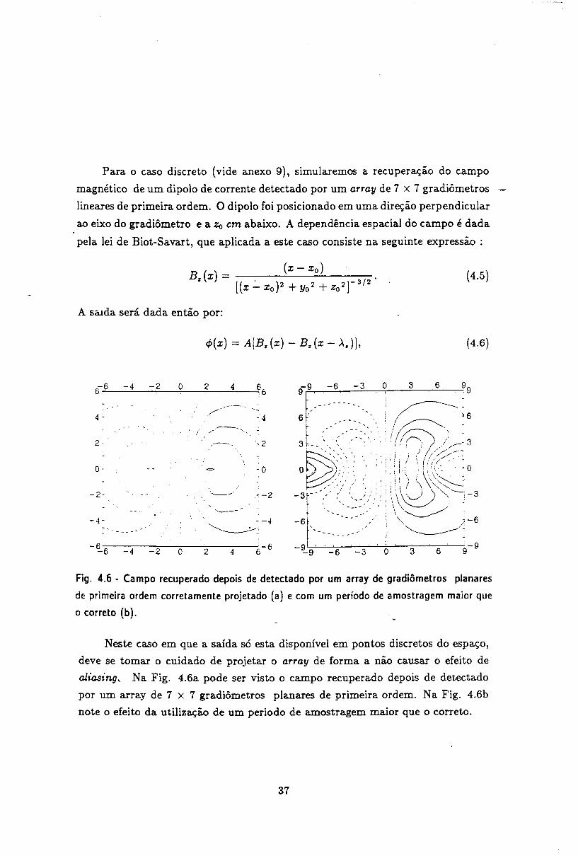
Para o caso discreto (vide anexo 9), simularemos a recuperação do campo

magnético de um dipolo de corrente detectado por um array de 7 x 7 gradiômetros

lineares de primeira ordem. O dipolo foi posicionado em uma direção perpendicular

ao eixo do gradiômetro e a Zo em abaixo. A dependência espacial do campo é dada

pela lei de Biot-Savart, que aplicada a este caso consiste na seguinte expressão :

B% ( x) = (x - xo)[(x .:...xo) 2 + Yo 2 + Zo 2r 3/2

A salda será dada então por:

(4.5)

(4.6)

~--,,....- ~,

2

2',- .

-4~

-~6

-4

-4

-2

-2

o

o

2

2

4

- ',2

-o

,"-2

4

Fig. 4.6 - Campo recuperado depois de detectado por um array de gradiômetros planares

de primeira ordem correta mente projetado (a) e com um período de a mostragem maior que

o correto (b).

Neste caso em que a saída só esta disponível em pontos discretos do espaço,

deve se tomar o cuidado de projetar o array de forma a não causar o efeito de

aliasing .. Na Fig. 4.680 pode ser visto o campo recuperado depois de detectado

por um array de 7 x 7 gradiômetros planares de primeira ordem. Na Fig. 4.6b

note o efeito da utilização de um periodo de amostragem maior que o correto.

37

,..,

5 DISCUSSAO

5.1 - Perspectivas

Com a recente descoberta de óxidos cerâmicos supercondutores em 1986

1987, materiais com temperaturas críticas acima de 100 K já estão bem estab

elecidos. De todas as prováveis e fJ.ntásticas aplicações que esses novos materiais

podem ter, as mais imediatas são precisamente o SQUID e os gradiômetros, dev

ido a sua operação com baixas correntes críticas. Portanto, imediatamente após

a descoberta, varios SQUIDs foram construídos por diversos grupos de pesquisa:

IBM [100], Hitachi Co~poration [101] , Tsukuba University [102], NBS/NIST [103]

and University of Strathclyde [104]. Até então estes dispositivos só serviram para

demonstrar os efeitos Josephson e de interferência quântica nestes novos super

condutores. Contudo, uma recente publicação [105] do grupo da IBM relata a

utilização de um SQUID imerso em nitrogênio líquido com um nível de ruído

similar ao do rf-SQUID para uma faixa de frequências acima de 10 Hz.

O grande progresso da medicina moderna se deve não tão somente ao desen

volvimento de novas tecnologias mas também ao desenvolvimento de uma série de

técnicas de obtenção de imagens que dão informações anatômicas e morfológicas

como a tomografia de raio-x computadorizada (CT scan), ressonância nuclear

magnética (NMR), tomografia por emissão de pósitrons (PET), ultrasonografia

colorida, etc ... O eletrocardiograma e o eletroencefalograma, embora extrema

mente úteis para o estabelecimento de diagnóstico clínico por darem informações

sobre a função do coração e do cérebro, utilizam até hoje os mesmos métodos de

registro e tratamento de sinal de um século atrás, quando da sua invenção. Um

dos grandes objetivos da Magnetocardiografia e da Magnetoencefalografia é permi

tir a obtenção da imagens dos processos funcionais de atividade elétrica cardíaca

e cerebral, difíceis de se obter através de eletrodos, com precisão temporal de

milésimos de segundo e espacial de poucos milímetros. Para isso atualmente está

sendo feito um grande esforço no desenvolvimento de sistemas'compostos de arrays

de gradiômetros, possibilitando assim, medidas simultâneas em vários pontos do

espaço [59-61].

38 -

5.1 - Conclusão

o objetivo desta tese foi o estudo da detecção de campos magnéticos fra

cos através da utilização de gradiômetros supercondutores acoplados à SQUIDs

e sua aplicação ao biomagnetismo. Um novo modelo teórico para descrição do

gradiômetro foi des(mvolvido com a obtenção da sua função de transferência es

pacial. Através desta função de transferência a atuação do gradiômetro sobre os

sinais detectados pode ser quantificada. Além disso, foi desenvolvido um proce

dimento para a medida experimental da função de transferência, onde as imper

feições no processo de construção do sensor podem ser medidas e avaliadas. Foi

proposta uma nova terminologia para descrição do gradiômetro ao invés de sua

descrição física. Nesta terminologia o gradiômetro ficará especificado pelo seu

rolloff, frequência de corte espacial e ganho máximo. Também foi generalizado o

método para projeto de gradiômetros onde novas configurações podem ser cons

truídas e testadas. A partir da obtenção desta função de transferência um método

para calibração teslà/volt do sistema foi desenvolvido, com uma precisão até então

não alcançada por outros métoGos e perfeitamente apropriado para utilização em

sistemas multicanais. Finalmente foi desenvolvido um algorítmo de desconvolução

para, a partir de sinais detectados com gradiômetros planares, recuperar o sinal

original como ele tivesse sido detectado somente por uma bobina. Este algorítmo

também pode ser utilizado para auxílio no projeto de arrays destes gradiômetros.

39

6 PUBLICAÇOES

6.1 Lista de Publicações

1. A Symmetric Third Order Gradiometer Without External Balancing for

Magnetocardiography, A.C. Bruno and P. Costa Ribeiro Cryogenics 23, 346

(1983).

2. Spatial Discrimination: An Alternative Approach, A.C. Bruno, P. Costa

Ribeiro, J .P. von der Weid and LR. Eghrari, Biomagnetism: Applieation

and Theory H. Weinberg, G. Stroink, and T. Katila (Eds.), Pergamon Press,(1985) p. 60

3. Discrete Spatial Filtering with SQUID Gradiometers in Biomagnetism, A.C.

Bruno, P. Costa Ribeiro, J.P. von der Weid and O.G. Sym~o, J. Appl. Phys.

59, 2584 (1986).

4. Spatial Fourier Transform Method for Evaluating SQUID Gradiometers, P.

Costa Ribeiro, A.C. Bruno, C.C. Paulsen and O.G. Symko, Rev. Sei. In

strum. 58, 1510 (1987).

5. Digital Filter Design Approach for Squid Gradiometers, A.C. Bruno and P.

Costa Ribeiro, J. Appl. Phys. 63, 2820 (1988).

6. Planar Gradiometer Input Signal Recovery Using a Fourier Technique, A.C.Bruno, A.V. Guida, and P. Costa Ribeiro, Biomagnetism '87 K. Atsumi et

aI. (Eds.), Tokyo Denki University Press (1988) p.454

7. Experimental Localization Ability of Planar Gradiometer Systems for Bio

magnetic Measurements, A.C. Bruno, V.Pizzella, G. Torrioli and G.L. Ro

mani, IEEE Trans. Magn. MAG-25 (2),1170 (1989).

8. Neuromagnetic Localization Performed by Using Planar Gradiometer Con

figurations, A.C. Bruno and G.L. Romani, J. Appl. Phys. 65, 2098 (1989).

9. Spatial Deconvolution Algorithm for Superconducting Planar GradiometerArrays, A.C. Bruno and P. -Costa' Ribeiro, IEEE Trans. Magn. MAG-25(2), 1216 (1989).

40

10. Spatial Fourier Technique for calibrating Gradiometers, A.C. Bruno, C.S.

Dolce, S.D. Soarez and P. Costa Ribeiro, Advances on Biomagnetism S.J.

Williamson (Ed.), Pergamon Press (in press)

11. Designing Planar Gradiometer Arrays : Preliminary Considerations, A.C.

Bruno and P. Costa Ribeiro, Advances on Biomagnetism S.J. Williamson

(Ed.), Pergamon Press (in press)

12. Spatial Fourier Method for Calibrating Multichannel.SQUID Magnetometers,

A.C. Bruno and P. Costa Ribeiro, (submetido ao Rev. Sci. Instrum.)

Estas publicações foram resultado de um trabalho de equipe, executado peloGrupo de Biomagnetismo no Laboratório da Matéria Condensada do Departa

mento de Física da Pontifícia Universidade Católica do Rio de Janeiro [1], [2],

[3], [4], [5], [6], [9], [10], [11] e [12] e pelo Grupo de Biomagnetismo do Istituto di

Elettronica dello Stato Solido, Consiglio Nazionale delleRicerche, Roma, Italia [7]e [8]. Todas estas publicações foram preparadas e escritas por mim.

6.2 - Resumo das Publicações

1. A Symmetric Third Order Gradiometer Without External Balancing for Magnetocardiography.Um estudo de viabilidade foi feito para a operação de um gradiômetro nãobalanceado e utilizado com o SQUID num ambiente não blindado magnetica

mente. Este artigo compara empiricamente as performances de gradiômetros

de segunda e terceira ordens e também apresenta um procedimento geral para

projeto de gradiômetros de terceira ordem.

2. Spatial Discrimination: An Alternative Approach.O tratamento de gradiômetros como filtros discretos espacias não recursivos

é proposto. Esta abordagem torna possível uma descrição analítica da função

de transferência do gradiômetro, que é a melhor caracterização de qualquerinstrumento de medida.

3. Discrete Spatial Filtering with SQUID Gradiometers in Biomagnetism.Gradiômetros de primeira, segunda e terceira ordens utilizados em biomag

netismo são analisados como filtros espaciais. As suas funções de transferência independentes do sinal a ser medido são apresentadas e suas amplitude e fase são analisadas. Desta forma, a distorçã.o introduzida no sinal

41

medido pode ser estimada. De forma a tratar o sinal sob mesmo formalismo,

a transformada de Fourier espacial de um sinal produzido por um dipolo decorrente é discutida.

4. Spatial Fourier Transform Method for Evaluating SQUID Gradiometers.

Um método simples para se medir a função de transferência espacial de um

gradiômetro é apresentado e o resultado comparado com o modelo teórico.

Baseado nesta abordagem, uma nova forma de se apresentar a performarice

de gradiômetros é r-ropostaj o fator de rejeição é expresso em dB e obtidodiretamemte da função de transferência medida.

5. Digital Filter Design Approach for Squid Gradiometers.Uma revisão do método tradicional de projeto de gradiômetros é feita. Um

modelo :lão recursivo digital para gradiômetros é apresentado, fornecendo

uma novo conjunto de parâmetros para a identificação do gradiômetro. Al

guns exemplos de gradiômetros são analisados usando o conjunto proposto.Um diferenciador é projetado para ser usado em conjunto com o SQUID.

É mostrado que o diferenciador tem a mesma rejeição para ruídos que umgradiômetrO- convencional mas tem uma maior sensibilidade ao sinal.

6. Planar Gradiometer Input Signal Recovery Using a Fourier Technique.O objetivo deste artigo é adaptar para gradiômetros planares o modelo de

filtragem espacial previamente desenvolvido para gradiômetros axiais. Este

modelo possibilitará a interpretação do sinal na saída do gradiômetro sem

ser necessário fazer qualquer suposição a respeito da fonte a ser medida.

7. Experimental Localisation Ability of Planar Gradiometer Systemsfor Biomagnetic Measurements.A possibilidade de localização de fontes biomagnéticas por gradiômetros pla

nares foi investigada. Um gradlômetro linear de fio supercondutor foi con

struído e testado. A localização foi feita em um modelo e em humanos. A

precisão da localização não foi afetada pelo uso da configuração planar.

8. Neuromagnetic Localization Performed by Using Planar Gradiometer Configurations.A discriminação espacial de gradiômetros axiais e planares foi comparada

utilizando um modelo de filtragem espacial. Medindo campos somatosensoriais evocados, dipolos equivalentes de corrente foram localizados utilizando

as configurações planares. As configurações foram obtidas combinando as

42 -

saídas de um sistema com quatro canais. Foi observado que com uma relação

sinal-ruído apropriada, o uso das configurações planares não afetou significa

tivamente a precisão dos resultados.

9. Spatial Deconvolution Algorithm for Superconducting Planar Gradiometer Arrays.Um modelo de filtragem espacial usado previamente para analisar gradiôme

tros é aqui usado para estudar arrays de gradiômetros planares de primeira

ordem. Como uma aplicação desta técnica um algoritmo de desconvolução do

sinal de saída com-a função de transferência do gra-liômetro foi desenvolvido,possibilitando assim a recuperação do sinal na entrada do array. A influência

de parâmetros como profundidade da fonte e a densidade de gradiômetros noarray é discutida.

10. Spatial Fourier Technique for Calibrating Gradiometers.Neste artigo é proposto um método geral de calibração de gradiômetros axlals

e planares. O método é baseado numa técnica de Fourier espacial e no fato

do gradiômetro poder ser modelado como um filtro espacial.

11. Designing Planar Gradiometer Arrays : Preliminary Considerations.

Neste artigo é iniciado um estudo sobre o projeto de arrays de gradiômetros

planares. Parâmetros como tamanho do array, e espaçamento entre osgradiômetros são discutidos.

12. Spatial Fourier Method for Calibrating Multichannel SQUID Systems.

Quando se utilizam sistemas multicanais para aplicações biomagnéticas, é de

extrema importância a estimação correta da calibração a tesla/volt de cadacanal, para se evitar erros quando da análise dos resultados. Neste trabalho

é proposto um método geral para calibração de sistemas multicanais que

fornece uma precisão melhor que 1%.

43

A

REFERENCIAS

[1] G.M. Baule and R. McFee, Am. Heart J. 66, 95 (1963).

[2] D. Cohen, E.A. Edelsack and J.E. Zimmerman, Appl. Phys. Lett. 16, 278

(1970).

[3] D. Cohen, J. Appl. Phys. 38, 1295 (1967).

[i] J.E. Zimmerman and A.H. Silver, Phys. Rev. 141, 367 (1966).

[5] A.H. Silver and J.E. Zimmerman, Phys. Rev. 157, 317 (1967).

[6] R.L. Fagaly, Supereonduetor Industry 2 (4), 24 (1989).

[7] D. Cohen, Seienee 175, 664 (1972).

[8] J.E. Zimmerman and N.V. Frederick, Appl. Phys. Lett. 19, 16 (1971).

[9] J.E. Opfer, Y.K.Yeo, J.M. Pierce and L.H. Rorden, IEEE Trans. Magn.

MAG-9, 536 (1974).

[10] M. Saarinen, P.J. Karp, T.E. Katila and P. Siltanen, Cardiovase. Res. 8,

820 (1974).

[11] D. Brenner, S.J. Williamson and L. Kaufman, Seienee 190, 480 (1975).

[12] D. Duret, P. Bernard and D. Zenatti, Rev. Sei. Instrum. 46, 474 (1975).

[13] B.N. Cuflin and D.B. GeseIowitz, IEEE Trans. Biomed. Eng. BME-24,242 (1977).

[14] J.P. Wikswo, Jr., AI? Conl. Proc. 44, 145 (1978).

[15~ S. Barbanera, P. Carelli, L Modena and G.L. Romani, J. Phys. E: Sei.

Instrum. 11, 297 (1978).

[16] M. Reite, J. Eldrich, J.T. Zimmerman and J.E. Zimmerman, Eleetroeneepha

logo Clin. Neurophysiol. 45, 114 (1978).

[17] D.E. FarreI, J.H. Tripp and R. Norgren, IEEE Trans. Biomed. Eng. BME26, 82 (1979).

[18] 1.R. Eghrari and P. Costa Ribeiro, Rev. Bras. Fis. 10 115 (1980).

[19] D.B. Geselowitz, IEEE Trans. Magns MAG-6, 346 (1970).

44

[20] F. Grynzpan and D.B. Geselowitz, Biophys. J. 13, 911 (1973).

[21] S.J. Williamson and L. Kaufman, Biomagnetism S.N. Erné et aI. (Eds.),

Walter de Gruyter, Berlin-New York, p.353 (1981).

[22] S. Barbanera, P. Carelli, R. Fenici, R. Leoni, I. Modeena and G.L. Romani,

IEEE Trans. Magn. MAG-l1, 849 (1981).

[23] P. Nicolas, D. Duret, D. Teszner and T. Tuomisto, n Nuovo Cimento 2D

(2), 184 (1983).

[24] D.F. Farrel, J.H. Tripp, G.M. Brittenham, E.H. Danish, J.W. Harris and

A.E. Traeht n Nuovo Cimento 2D (2), 582 (1983).

[25] P. Costa Ribeiro, I.R. Eghrari, A.C. Bruno, C.A. Bastos, J .P. von der Weid,

A.P. Picon e E. Joaquim, Anais do VIII Cong. Bras. Eng. Biomed. p.294

(1983).

[26] D. Cohen and L. Kaufman, Circulation Res. 36, 414 (1975).

[27] D. Cohen, E. Lepeschkin, H. Hosaka, B.F. Massel and G. Myers, Elutrocar

diology J. 9, 398 (1976).

[28] M. Saarinen, P. Siltanen, P.J. Karp and T.E. Katila, Ann. Clin. Res. 10

(21), 1 (1978).

[29] D.E. Farrel, J.H. Tripp and R. Norgren, IEEE Trans. Biomed. Eng. BME

21, 345 (1980).

[30] R. Fenici, G.L. Romani and R. Leoni, n Nuovo Cimento 2D (2), 280 (1983).

[31] I.R. Eghrari, E. Costa Monteiro, P. Costa Ribeiro, J. P. von der Weid, P.M.

Oliveira and A. Paes de Carvalho, n Nuovo Cimento 2D (2),346 (1983).

[32] M. Reite, J.E. Zimmerman, J. Eldrich and J.T. Zimmerman Electroencepha

logo Clin. Neurophysiol 40, 59 (1976).

[33] J.R. Hughes, J. Cohen, C.I. Mayman, M.L.Scholl and D.E. Hendrix, J. Nwrol. 211, 79 (1977).

[34] D.E. Farrel, J.H. Tripp, R. Norgren and T.J. Teyler, Electroencephalog. Clin.

Neurophysiol. 49, 31 (1980).

[35] L. Kaufman, Y.C. Okada, D. Brenner and S.J. Williamson Int. J. Neurosá.

15, 223 (1981).

[36] G.L.Romani, S.J. Williamson and L. Kaufman, Science 212, 1339 (1982).

45

[37] R.M. Chapman, R. Ilmoniemi, S. Barbanera and G.L. Romani, Electroen

cephalog. Clin. Neurophysiol. 58, 569 (1984).

[38] H. Hukkinen, V. Kariniemi, T.E. Katila, H. Laine, R. Lukander and P.

Makipaa, Am. J. Obstet .. Gynecol. 125, 1115 (1976).

[39] W.H. Barry, W.M. Fairbank,--D.C. Harrison, K.L. Lehrman, J.A.V. Malmivuo

and J.P. Wikswo,Jr., Science 198, 1159 (1977)

[40] D.E. Farrel, J.H. Tripp, R. Norgren, Proc. SPIE 167, 173 (1978).

[41]. P. Siltanen, T. Poutanen, T. Katila, M. Seppanen and T. Varpula, n Nuovo

Cimento 2D (2), 301 (1983).

[42] D.S. Barth, W.H. Sutherling, J. Engel and J. Bea~ty, Science 218, 891 (1982).

[43] L Modena, G.B. Ricci, S. Barbanera, R. Leoni, G.L. Romani and P. Carelli,

Electroencephalog. Clin. Neurophysiol. 54, 622 (1982).

[44] G.M. Brittenham, D.E. Farrel, J.W. Harris, E.S. Feldman, E.H. Danish,W.A. Muir, J.H. Tripp, J.N. Brennan and E.M. Bellon, n Nuovo Cimento

2d, 567 (1983).

[45] D.F. Rose, S. Sato, P.D. Smith, R.J. Porter, W.H. Theodore, W. Friauf, R.

Bonner and B. Jabbari, Ann. Neurol. 22, 348 (1987).

[46] W.W. Sutherling, P. Crandall, L.D. Cahan and D.S. Barth, Neurology 38,

778 (1988)

[47] P. Costa Ribeiro, A.C. Bruno, E. Parenet Ribeiro, J.S. do Carmo, E. Costa

Monteiro and A. Fonseca Costa, Advances in Biomagnetism, S. J. Willianson

(Ed.) in press (1990).

[48] N. Tepley, G.L. Barkley, J. Moran, R.T. Simkins and K.M.A. Welch, Ad

vances in Biomagnetism, S. J. Willianson (Ed.) in press (1990).

[49] J.P. Wikswo,Jr., J.P. Barach and J.A. Freeman, Science 208, 53 (1980).

[50] M. Leifer, N. Capos J. Griffin and J. Wikswo,Jr., n Nuovo Cimento 2D (2),

266 (1983).

[51] E. Costa Monteiro, A.C. Bruno, S.R.W. Louro, P. Costa Ribeiro and A.

Fonseca Costa, Phys. Med. Biol. 32, 65 (1987).

[52] Y.C. Okada, M. Lauritzen and-.C. Nicholson, Brain Res. 442, 185 (1988).

[53] Y.C. Obda and C. Nicholson, Biophys. J. 53, 723 (1988).

46

[54] E. Costa Monteiro, S.R.W. Louro, A.C. Bruno and P. Costa Ribeiro, Biomag

netism '87 K. Atsumi et a!. (Eds.), Tokyo Denky University Press, Tokyo,

p.310 (1988).

[55] R. Ilmoniemi, R. Hari, K. Reinikainen, Eletroeneephalogr. Clin. Neurophys

io1., 58, 467 (1984).

[56] S.J. Williamson,M. Pelizzone, Y. Okada, L. Kaufman, D.B. Crum and J.R.

Madsen, Biomagnetism: Theory and Applieations, H. Wienberg et a!. (Eds.),

New York, Pergammon Press, p.46 (1984).

[57] G.L. Romani, R. Leoni and C. Salustri, SQUID 85: Supereondueting Quan

tum lnterference Deviees and their Applieations, H.D. Hahlbohn et a!. (Eds.)

Berlin-New York, Walter De Gruyter, p.918 (1985).

[58] J. Knuutila, S. Ahlfors, A. Ahonen, J. Hallstron, M. Kajola, O.V. Lounasmaa,

V. Vilkman, and C. Tesehe, Rev. Sei. Instrum. 58, 2145 (1987).

[59] H.E. Hoenig, G. Daalmans, W. Folberth, H. Reiehenberger, S. Sehneider, and

H. Seifert, Cryogenies 29, 809 (1989).

[60] M. Kajola, S. Ahlfors, G.J. Ehnholm, J. Hallstrom, M.S. Hamalainen, R.J.Ilmoniemi, M. Kiviranta, J. Knuutila, O.V. Lounasmaa, C.D. Tesehe, and

V. Vilkman, Advanees on Biomagnetism, S.J. Williamson (Ed.), Pergamon,New York, (1989). in press

[61] Biomagnetie Teehnologies, Ine., 4174 Sorrento Valley Blvd., San Diego, CA92121, USA.

[62] G.L. Romani, S.J. Williamson, and L. Kaufman, Rev. Sei. lnstrum. 53,

1815 (1982).

[63] SQUID'80, Supereonduding Quantum lnterferrenee Deviees and Their Ap

plieations, H.D. Hahlbohm and H. Lübbig (Eds.), Walter de Gruyter, BerH.l,(1980).

[64] SQUID'85, Supereondueting Quantum lnterferrenee Deviees and Their Ap

plieations, H.D. Hahlbohm and H. Lübbig (Eds.), Walter de Gruyter, Berlin,(1985).

[65] B.D. Josephson, Phys. Lett. 1, 251 (1962).

[66] A. Barone and G. Paterno, Physies and Applieations of the Josephson Effeet,

Willey, New York, (1982).

47

[67] A.P. Picon, I.R. Eghrari e P. Costa Ribeiro, Rev. Bras. Fis. 11, 863 (1981).

[68] J.E. Zimmerman, P. Thiene and J.T. Harding, J. Appl. Phys. 41, 1572

(1970).

[69] J.E. Zimmerman Cryogenics 12, 19 (1972).

[70] J. Clarke, W.M. Goubau and M. B. Ketchen, J. Low Temp. Phys. 25, 99

(1976).

[71] C.D. Tesche and J. Clarke, J. Low Temp. Phys. 29, 301 (1977).

[72] M. B. Ketchen, IEEE Trans. Magn. MAG-17, 387 (1981).

[73] V. Foglieti, W.J. Gallagher, M.B. Ketchen, A.W. Kleinsassen, R.H. Koch

and R.L. Sandstrom Appl. Phys. LeU. 55, 1451 (1989).

[74] V. Kelhã, J. Pukki, R. Peltonen, A. Penttinen, R. Ilmoniemi and J. Heino,

IEEE Trans. Magn. MAG-18, 260 (1982).

[75] G. Stroink, C. Purcell, F. Brauer and B. Blackford, n Nuovo Cimento 2D(2), 195 (1983).

[76] G.W. Sullivan and E.R. Flynn, B~'omagnetism'87 K. Atsumi et aI. (Eds.),

Tokyo Denky University Press, Tokyo, p.486 (1988).

[77] John R. Reitz and Frederick J. Milford, Foundations of Electromagnetic The

ory, Addison-Wesley, Reading MA, (1967).

[78] J.H. Claassen, J. Appl. Phys. 46, 2268 (1975).

[79] J. Vrba, A.A. Fife, M.B. Burbank, H. Weinberg and P.A. Brickett, Cano J.

Phys. 60, 1 (1982).

[80] J.A. Overweg and M.J. Walter-Peters, Cryogenies, 18, 529 (1978).

[81] F. W. Grover, Induetanee Calculation,5, Dover, New York (1962).

[82] R. Merritt, C. Purcell, and G. Stroink, Rev. Sei. Instrum. 54, 879 (1983).

[83] J. Mallinson, J. Appl. Phys. 37, 2514 (1966).

[84] D.G. Smith, Am. J. Phys. 48, 739 (1980).

[85] J. Storey, n Nuovo Cimento 2D (2), 153 (1983).

[86] J. Sarvas, Phys. Med. Biol. 32, 11 (1987).

[87] B.N. Cuffin, Phys. Med. Biol. 32, 33 (1987).

48

[88] A. Antoniou, Digital Filters Analysis and Design, McGraw-Hill, New York,

(1979).

[89] M. 8chwartz and L. 8haw, Signal Processing, McGraw-Hill, Tokyo, (1975).

[90] A.V. Oppenheim and R.W. 8chafer, Digital Signal Processing, Prentice

Hall, New Jersey, (1975).

[91] P. Costa Ribeiro, 8.J. Williamson, and L. Kaufman, IEEE Trans. Biomed.

Eng. BME-35, 551 (1988).

[92] M.B. Ketchen, W.M. Goubau, J. Clarke and G.E. Donaldson, J. Appl. Phys.

49, 4111 (1978).

[93] V.J. de Wall and T.M. Klapwijk, Appl. Phys. Lett. 41, 669 (1982).

[94] P. Carelli and V. Foglieti, J. Appl. Phys., bf 54, 6065 (1983).

[95] F. Wellstood, C. Heiden and J. Clarke, Rev. Sei. Instrum. 55, 952 (1984).

[96] G.J. van Nieuwenhuyzen and V.J. de Waal, Appl. Phys. Lett. 46, 439

(1985).

[97] M.B. Ketchen, IEEE Trans. Magn. MAG-23, 1650 (1987).

[98] M. Koyanagi, N. Kasai, K. Chinone, M. Nakanishi, 8. Kosaka, M. Higuchi

and H. Kado, IEEE Trans. Magn. MAG-25 (2), 1166 (1989).

[99] C.T. Chen, One Dimensional Digital Signal Processing Dekker, New York

(1979).

[100] R.H. Koch, C.P. Umbach, G.L. Clark, P. Chaudhari and R.B. Laibowitz,

Appl. Phys. Lett. 51, 200 (1987).

[101] H. Nakane, T. Nishino, M. Hirano, K. Takagi and U. Kawabe, Extended

Abstracts of the 1987 Internatt"onal Superconductt"vity Electrom"cs Conference

ISEC'87, Japan 80ciety of Applied Physics, Tokyo, p. 411 (1987).

[102] r. Iguchi, A. Sugishita and M. Yanagisawa, Japan. J. Appl. Phys. 26, LI021

(1987).

[103] J.E. Zimmerman, J.A. Beall, M.W. Cromar, R.H. Ono, Appl. Phys. Lett.

51, 617 (1987)

[104] G.B. Donaldson, Extended Abstracts of the 1987 International Superconduc

tivity Electronics Conference ISEC'87, Japan Society of Applied Physics,

Tokyo, p. 10 (1987).

49

[105] R.H. Koch, W.J. Gallagher, B. Bumble and W.Y. Lee, Appl. Phys. Lett. 54,

951 (1989).

50

ANEXO 1

A feasibility study is being carried out on the operation of a SQUID gradiometer

without any ba/ancing techniques in a non-shielded environmenr. This paper compares

empirica/ly the performances of second and third order gradiometers; it also presents a

general procedure for the design of third order gradiometers, taking into account themeasured spatia/ dependence of the magnetic field of the human heart.

The performance of a third order gradiometer is very promising for a noisyenvironment; it has a better low frequency noise rejection than the second order gradio

meters tested, and needs no external ba/ancing.

A symmetric third arder gradiometer without

external balancing for magnetocardiography

A.C. Bruno and P. Costa Ribeiro

Key words: superconducting devices, SQUID gradiometer, magnetocardiography

Since the late sixties when SQUID magnetometersbecame available. various types of biomagnetic fields can bemeasured. Due to the weakness af these fields in the presenéeof environmental noise. various techniques have beendeveloped to increase the signal-to-noise ratio especially inclínica! applicarions. Basically there are two ways ofrejecting heavy urban magnetic noise: taking measurementsin magnetically shielded raoms.1,2 or by using gradio-meters which will perforrn spatial discrimination againststray magnetic fields from distant sources.3

The latter approach has been extensively reported inrecent papers.4•5•6 However. to' attain a good performancein the low frequency region. complicated balancingtechniques 7.8 have to be used to compensate against imperfections in the construction of the gradiometer.

Our approach does not rely on such balancing techniques hence the overall system is easier to constructand is free from trims, tabs. helmholtz coils, etc. Also oursystem does not require balancing after each new heliumtransfer.

The noise problem

The magnetic noise generated by distant sourcescan be spatially approximated by the fust two terrns of aTaylor's series expansion:

õBz(zo)Bz(z-zo)=Bz(zo) + --(z-zo) (I)

õz

where Zo is the origin of the expansion.A generation of first aI).dsecond order gradiometers

has been designed based on this assumption. However.unshielded enviranments aften have noise sources which

cannot be modelled only by the first two terms of theexpansion above. This is the case when noise sources getdoser to the gradiometer. 50, terrns Iike the second orderderivative component ought to be added to thisexpansion:

õBz(zo) õ2 BzCzo) (Z_ZO)2

Bz(z) = Bztzo) + ,,- (z-zo) + - ~ -:2(2)

If a second order gradiometer is used to measure theheart's magnetic field in such an environmem, the noisepresent in the magnetocardiogram is a function of thefield. gradiem imbalance and second order componems aimagnetic noise. which are not rejected by this type of gradil"meter. 50. it was decided to increase the arder of the

gradiometer without using balancing techniques, to diseoverto what extent second order components af magnetic noiseare presem in the magnetocardiogram.

Spatial dependence of the magnetic field of thehuman heart

The next step in the design is to find the spatial depenodence of the heart's magnetic field in the direction of thegradiometer axis which is usually placed perpendicular tothe chest plane. The decrease in the heart's magneticfield (QRS peak-to-peak amplitude falloff) in the directionnormal to the chest wall is actually much slower than thedecay of a dipolar source. which is commonly used as anapproximation for design purposes. This can be checkedby using the results reponed by Cohen et alI. wheremeasurements with a single coil magnetometer were performed at six different distances fram the chest in two

different positions. Plotting their measured QRS peak-topeak amplitudes versus the distance. Z. fram the chesI. itwas found that the amplitude falloff can be approximatelvdescribed by an empirical K/Z"= dependence, where K is ~eonstant. Such a dependem:e has no physical meaning sincethe origin of the Z coordinate has been taken at the chestwall. which is far fram the heart sources, however it is agood field description for design purposes.

With a slow falloff, it is not possible to neglect t hemagnetic signal presem at the more remote coils of thegradiometer. which disproves the usual assumption thatmost af the Oux coupled to the gradiometer is the inducedtlux at the lowest coil. the sensing coi!. For instance. usingt he K/Zl/, field dependence. for a~conventional second ordergradiometer 7 with an overalllength of 20 cm and its sensingcoil at a distance af 1.1 em fram the chest wall. a net

magnetic tlux of anly 60':'~af the induc~d nux at the sensingcoil is produced.

324

0011-2275/83/060324-{)3 $03.00 © 1983 Butterworth & Co (Publishersl Ltd.

CRYOGENICS. JUNE 1983

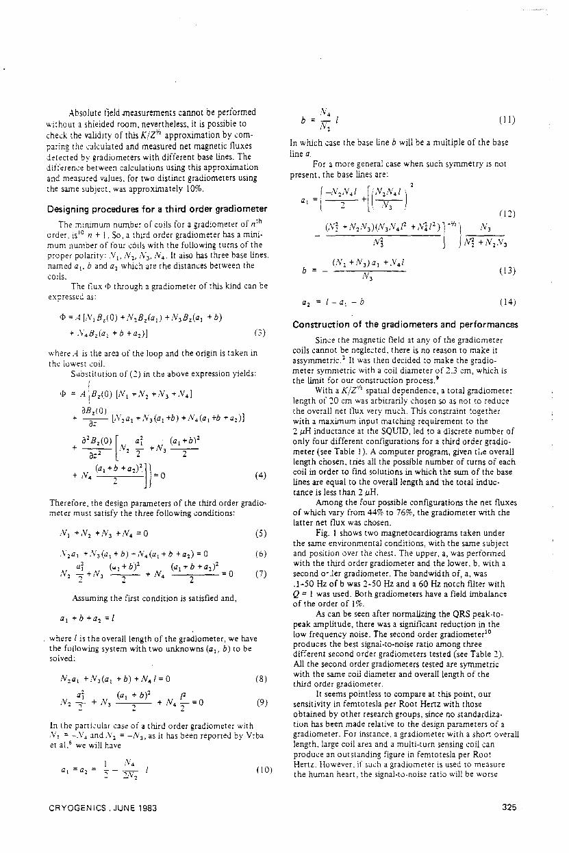
(14)

(13 )

( 12)

til)

(Nl +NJ)al +N4/

NJ

(,"1 +NlNJ)(NJN4f"l. +i\'1Il)]-lh} ~N5 I\'1 + N l'V J

b =

In which case the base Une b will be a multiple of the baseline a.

For a more general case when such symmetry lS notpresent, the base Unes are:

").

_ r -N").N41 [('Nll'vf41 ')al-\ .., +-Y--\ - . 1 J ,Designing procedures for a third order gradiometer

The minimum number of coils for a gradiometer oi nth

order. is10 n + 1.50, a third order gradi;meter has a minimum number of four cóils with the folJowing turns of theproper polarity: .VI•N2• NJ• N4. It also has three base lines,namcd ai. b and a2 which are the distances between thecoils.

The f1ux (P through a gradiometer of this kind can beexpressed as:

Absolute field .rneasurements cannot be performedwithout a shielded room, nevertheless, it is possible to

check the validity of this KIZ'tí approximation by comparing the cakulated and measured net magnetic fluxesdetected by gradiumeters with different base lines. Thedifference between calculations using this approximationand measured values, for two distinct gradiometers usingthe same subject, was approximately 10%.

Construction of the gradiometers and performances

Since the magnetic f1eld at any of the gradiometercoils cannot be neglected. there is no reason to make itassymmetric.l It was then decided to make the gradiometer symmetric with a coil diameter of 2.3 cm, which isthe limit for our construction process.9

With a K/Z1/' spatial dependence, a total gradiometerlength of 20 cm was arbitrarily chosen so as not to reducethe overaU net tlux very much. This constraint togetherwith a maximum input matching requirement to the2 tlH inductance at the SQL'lD, led to a discrete number ofonly four different configurations for a third order gradiometer (see Table I). A computer program, given ti,e overalllength chosen, tries aJ! the possible number of turns of eachcoi! in order tO find solutions in which the sum of the base

lines are equal to the overalllength and lhe total inductance is less than 2 tlH.

Among the four possible configurations the net fluxesof which vary from 44% to 76%, the gradiometer with thelatter net f1ux was chosen.

Fig. 1 shows two magnetocardiograms taken underthe same environmental conditions, with the same subjectand position over the chest. The upper, a, was performedwith the third order gradiometer and the lower, b, with asecond o·ler gradiometer, The bandwidth of, a, was.1-50 Hz of b was 2-50 Hz and a 60 Hz notch filter withQ :: I was used. 80th gradiometers have a fjeld imbalanceof the order of 1%.

As can be seen after normalizing the QRS peak-topeak amplitude, there was a significant reduction in thelow frequency noise. The second order gradiometer10produces the best signal-to-noise ratio among threedifferent second order gradiometers tested (see Table 2).Ali the second order gradiometers tested are symmetricwith the same coil diameter and overalllength of thethird order gradiometer.

It seems pointless to compare at this point, oursensitivity in femtotes]a per Root Hertz with thoseobtained by other research groups, since no standardiza·tion has been made relative to the design parameters of agradiometer. For instance. a gradiometer with a short overalllength, large coil are:! and a multi-turn sensing coil canproduce an outstanding figure in femtotesla per RootHertz. However, if such a gradiometer is used to measurethe human heart, the signal-to-noise ratio will be worse

(9)

(10)

(8)

(4)

N4

~ - 7..Nl

+b)+N41=0

aI (al+b? PN, - + NJ ---- + N4 - :: O

- .., 2 2

where A is the area of the loop and the origin is taken int he lowest coiJ.

Substitution of (2) in the above expression yields:(

<P = A,Bz{O) [NI +N2 +NJ +N4]

aBzlO)

+ ---az- [N").a1 +NJ(al +b) +N4(al +b +a2)]

a2Bz(0) [ai (aI +b)2+ --- N2 - +NJ ---

~2 2 2

(al+b+a2)2]}+ N4.., = O

.i.

where I is the overalllength of the gradiometer, we havethe following system with two unknowns (aI. b) to besolved:

Assuming the first condition is satisfied and,

Therefore, the design parameters of the third order gradiometer must satisfy the three following conditions:

In the particular case of a third order gradiometer withNI = -.V~ andN"). = -1VJ, as it has been reponed by Yrbaet al,6 we wiU have

<P =.4 [NIBz(O) +NlBz(ad +NJBz(al + b)

+ .V4Bz(a1 +b +a2)] (3)

CRYOGENICS . JUNE 1983 325

Tabte 1. A 3rd order gradiometer configurations

No of turns

3rd orderBase lines.

of each cail.gradiometer.Inductance.a,

b a2N,N2N3N4Net flux /olH

5.00

10.005.001-22-144% 0.9

5.36

11.553.091-23-245% 1.5

6.67

6.676.671-33-147% 1.7

3.09

11.555.362-32-176% 1.5

Table 2.

2nd order gradiometer configurations tested

No of turns

2nd orderBase lines

of each cailgradiometer.Inductance,a,

b a2N,N2N3N4Net flux /olH

3.00

14.00 3.001-1-1146% 0.4

10.00

0.010.001-1-1160% 0.6

4.67

12.33 3.002-3 2-196% 1.5

'·••'••••I••••!....I'••·,••••,••••'·••·j· ..·12~P.T" .. ·, ..·,I,,··,·· .. ,.... ,.... ' .....[.... ,.... ,.... ,

o

b

Fig. 1 Comparison betVlleena - third and b - seeond ordergradiometer performanees under the same eonditions

than that obtained by a gradiometer optimized for thatkind of measurement.

The perfonnance of the third order gradiometerproves that second order components of magnetic noise areindeed present in our environrnent. Regarding the reductionof the low frequency noise and sensitivity to the heart's

326

magnetic field, it seems worthwhile to carry on with ourstudies, optimizing the overalllength of the gradiometerand the coil area.

We would like to thank LR. Eghrari and Df. O.Symko for helpful suggestions.

Authors

The authors are at the Dept de Física, PontificiaUniversidade Catolica de Rio de Janeiro, CP 38071, Rio de

Janeiro, Brazil. Paper receíved 2 March 1983.

Réferences

Cohen, D. Report of the Low Field Group: The ~lagnetocardiograrn MIT Deeember (1975)

2 Zimmerman, J.E. Journ Appl Phys 48 (1977) 7023 Zimmerman, J.E., Frederiek. N.V.Appl Phys Letters 19

(1971)164 Barbanera, S., et alo Biomag Measurements Ere. Biomagnetism.

S.N. Erné, H.D. Hahlbohm. H. Lübbig (Eds). Berlin. :'-IewYork (1981) 139

5 Barbanera, S., Carelli, P., Fenici, R., Leoni, R., Modena, 1.,Romani, G.L.IEEE Trans Magnerics MAG-17 (1981) 849

6 Vrba, J., Fife, A.A., Burbank. M.B., Weinberg, H., Briehett.P.A. Can Journ Phys 60 (1982)

7 Opfer, J.E., Yeo, Y.K., Pieree, J.M., Rorden, L.H.IEEETransMagnerics MAG-9 (1974) 536

8 Overweg, J.A., Walters-Peters, M.]. Cryogenics 18 (1978)529

9 Eghrari, I.R., von der Weid, J.P., Costa Ribeiro, P., Symko, O• On the reeording ete., Biomagnetism, S.N. Erné, H.D. Haulbomn,

H. Lübbig, (Eds) Berlin-New York (1981) 30410 Karp, P., Duret, D. Journ Appl Phys51 (1980) 1267

CRYOGEN1CS . JUNE 1983

ANEXO 2

~~'7~~~"";'

SERViÇO DE BIBLiOTECA E !~HO;~Mf.ÇAO - ffaseflSICA

SPATIAL DISCRIMINATIOth AR ALTERNATIVE APPROACH

A.C. Bruno, P. Costa R~beiro, J.P. voU der Weid and I.R. Eghrari

Departamento de Fisica, Pontificia Universidade CatolieaCx.Postal 38071, Rio de Janeiro - RJ. BRASIL

ABSTRACT

The treatment of gradiometers as nonreeursive diaerete apatial filters ia a highpaas eonfiguration ia propoaed. Thia approaeh makea poaaible ao acalytical deacription of the gradiometer'a trsnsfer funetion vhieh ia the major characterization of any inatrument of messurement.

KEY\JORDS

SQUID. Gradiometer. Digital Filtering.

INTRODUCTION

After the introduction of the SQUID •.it vas the use of gradiometera aa aeaaiagcoils (Zimmerman, 1971), thereby avoiding the expensive ahielded roama (Coheu,1975), that led to an inereasing number of laboratoriea studyiag Biomagneti~.Different types of grsdiometers (symmetr1c, assymmetric, vith different ordera,sizes and areaa) have been built 1n many laboratoriea. The main goa1 in deaigning a gradiometer haa alvays been to aehieve the largest signal-to-noiae retio,and the fact that each group usea a particular type of gradiometer haa aot been Isource of trouble. Nevertheleaa, vith the need to compare data betveen groups,thia lsek of atandardization muat be overeome. Ia cardiomagnetiem, vhere themagnetic field of the extended eouree falle off less rapidly than the field of Isingle eurrent dipole, thia problem ia especially important. In flet, vith lucha elov falI off oí the field, not only the lovest coil, but the upper coill inthe gradiometer contribute to the aignal. It vould therefore, be intereating tohave an analytieal description of this deviee in order to characterize it, enablingone to be eonscious of the amount of diaturbanee introduced in the eignal.

GRADTOMETERS SENSING COILS

Traditional1y, the equations that define a Nth order gradiomerer can be found byeonsidering the total fluxo ~(t). induced in N+1 eoila connected in aeriel,

(1)

.vhere %i ia the diatance from the ith-coil to the origin, B (z) is the componentof the magnetic field perpendicular to the coil'a plane, Ana f(t) incorporatea the

time dependence of the fluxo tach coil co~siyta of nâ turna (poaitive or negative)taken by a1mp'icity vith the aame area A. Expanding % in TayIor aeries about %0

and calling bf- %i - %0 the distance betveen each coil and the lovest one. expreaaion (1) can 5e gIven ln matrix form:

68 BIOMAGNETISM: APPLlCATIONS ANO THEORY

vhere the y'S are the non zero diagqnal terms o~ the squar_ matrix. The similaiity betveen a gradiometer and an electronic filter is stressed by the usual procedure to check gradiometer'a unbalance. To measure the canceIlation of the firattvo terma of the gradiometer matrix in a second order gradiometer, a constant fieldand a conatant Rradient fleld are uaual1y applied to the syatem. That routine ia

(G)

(2)

(3)

f(t)B (2)(% )

% o

o

o

no+nl+n2+" •

n1b1+n2b2+ •••

O -J

Thia expreaaion ia similar to that of e.g. a se~ond order gradiometer,.O

OHB ('t )II OZ ! o

OB(1)(%o)

2

2 O

tn1b1 n2b2 -I(5)

-2-+

-- + ..•

B;2) (-o)Yll(2) (to)tIIO

F(t) - !Cjw t

e nn-O

n

vould be:

,..O ólICo

OO

OCI

C2

C2

-

Thti1iagonal matrix representa the effect on the fieId, (Bt), and ita deriv3tives,(Bt ), at the lovest coil, (to), due to the gradiometer. If the gradiometer isdesigned ao that the firat diagonal terma in the square matrix are cancelled. thenthe contrfbution of a far aource ia diminished but the near source signal is alsoeffected.

Such approach ia similar- to the classical electronic filtering of a time dependentaignal. For instance, the matrix representation of an ideal high-pass filter acting on a function F(t) expanded in Fourier series,

~(t) - A [111 •••]

-.l~

"1"1:

'1X!I"I!!,c~..",,·~

-~-

BIOMAGNETISM: APPLlCATlONS ANO THEORY 69

equivalent to determloing the tran.fer functioo of an electronic filter by coooectlog to it •• ine vave generator and mea.uring the output inten.ity for eacb frequency. Nevertheleas, up to thi. point, the analog, betveen a grsdiometer &Dd afilter i. confloed only to the matrlx repre.entation. S1Dce the Taylor polynomiala do not constitute an orthonormal baaia, the gradiameter'a tranafer functioa

cannot be derived by uaing the Taylor approach.

C1V.DIOKETER, A NONRECURSIVl DISCUTE FILTU

A gradibmeter detecta a .ignal that ,t. a contlou~ue function of time. Tha e-.plLa.takee plece at diacrete pointa in .paca corre.ponding to the poaitioo of tha coile.The net eignal ~eesured ie a veighted aum of these eampled ~aluea. Thua, it ia

eimple to apply digital .ign~l proceaaing techniquea (Lehmann, 1983) (Schvart&,1975) to handle thia problem. The output of • nonrecuraive or ~ving-.~er.gefilter can be defined by the vell knovn expreasion

(6)

This operstion defines a nev aet of discrete numbers Ym Erom a aet of óumbera x.corresponding to values of a variable aampled at constant intervala. Differentfilters correspond to different coeficienta h. Although it ia common to fit amonotonic function like the l/r' or 1/r2magnetic field fram a magnetlc or electriccurrent dipole by a polynomyal expanaion, it ia posaible to deacribe the field bya Fourier expansion. The discrete Fourier transform of the aignal at aase inetantof time viII be

(7)

vhere k is the vave number and ~a ia the distance betveen tvo succesai~e e••plingpoints.

Assuming that the diatances bi can alI be expressed aa multiplea of ~a' that ie"

(8)

8ibeing integera and ~s being therefore jU5t the maximum common di~iaor of alItne bi, the signal detected by the gradiometer viII be given by:

ia the number of tuma of each coi1 and xi i.of time at the ith coil. The tranafer func

obtained by taking the Fourier tranafora of

vhere N+l ia the number of coila, n

the magnetic flux at a given instanttion, defined by Y(k) - H(k) À(k), iathe sequence of filter coefficients:

(9)

N

H(k) - t "ii-O

A far aource of field (background noiae) viII mainly have lov frequency componente,(X(k) viII be large near k-O) vhile a near aource (aignal) viII have high frequencycomponents.

Fl~ure l(a), Magnitude of the gradiometers' transfer functlon and (b) thelrache~~tle geometries.

The Ipat1al d11cr1m1nat10n v111 be ach1eved by mak1ng the movlng ftverage f11ter

(grad10meter) 1ntot~ h1gh-paal f11ter. It 11 lntereat1ng to note that the dealgneond1t10na for I N order grad10meter, obta1ned by the trad1tlonal Taylorapproaeh (Karp, 1980),

(12)

(11)

3"

( bl

I"

a-O, ••• ,N

11 ~ !: 2-"

III III. - .-

- oNr1-0

(a I

IHlkl!

BIOMAGNETISM: APPLlCATIONS AND THEORY

CHOOSING GRADI0HETERS' DESIGNS

A:l the tronafer funetlous are high-paa9 flltera vith the gradiometera of higherorder more effeetively Bttenuatlng 10v frequeney baekgr~und noiae.For frequenc1ea larger than 0.3 em-I, the Fourier eomponentB of the aignal are very8mo11, representing only a fev pereent of the total power apeetrum. Thia iaparticularly true for the eardiae magnetle signa1. (Bruno, 1984).The ehoice betveen grad10metera of diffecent order viII then be determlned by thebehavlour of the tronafer functiona for frequenclea belov 0.3 em-I. For a aeverebAckground noifte envlronment due to not toe dlatant soureea. figure 1 lndieatea

Th1a alternative approaeh to the atudy of grad10metera providea a nev tool foropt1m1z1ng the eholee of gradlometer parameter. for eaeh speelfle situation, ai 1s111uatrated by f1gures 1 and 2 and the br1ef out1ine presented belov. Figure 1ahowa the tranafer funetlon magnitude H(k) aa def1ned by (10) for f1rst, aeeondand th1rd order aymmetr1e grad10metera. The gr~diometers' total length are the

lame (IDem) and therefore the aampling period Às are respeetively 10, 5 and 2.5 em.

Aa 1a the eaae for the diaerete Four1er_~ranaform, the h1ghest me~n1ngful frequeney ia n/Àa or 0.31, 0.62 and 1.26em reapeetively.

ftreobta1ned 1n the Fourler approaeh by 1mposlng:

30, H(k)1 .. !

--- - O 10-0 •...•Na .3k k-O

70

BIOMAGNETISM: APPLlCATIONS ANO THEORY nthe ule of I third order gradio~eter even if the Ilgnal li alio draltleally redueed.

The magnitude of the transfer funetion IX(k)f for differeat grad1o~terl delerlbed1n llterature are Ihovn in flgure 2. Their areal hav. beea normallzed to uaityfor almplielty. The use of a flrlt order gradlo~ter vith a large baa. 110.(curve 1) 1s perfectly justlfled in a suburban area vhere the backgrouad oolle ilvery lav. The cardlac lignal amplltude vlll therefore, be large since for lotermedlate frequencles the transfer fuactlon amplitude li large. The be.t ehoie. ofthe gradiometer lengths ean be luggested by eomparlng tva lecond order grad1~t.r.(curves 2a and 2b). For short lengths (large w/~ ) (curve 2a) the fllter ~r.efflelently attenustes lov frequeney c~poneotl, Ravlng a large backgrouod aoia.rejeetlon, but also reduees the slgnal amplltude by attenuatlog the lotermedlat.frequeneies. This short gradiometer ls indeed a good choiee for studlel of br.inevoked fields vhen the gradiometer is aear a l/rz souree vhose signal containa

high frequency components in the signal.

•0

2.0

Figure 2. SQUID Cradiometers' Traasfer Funetions:(I) Flrst Order Cradlameter(total Iength IOcm) (Saarlnen, 1978); (2a) Second Order Cradlameter (totsl leagth6.4em) (Willismson, 1978): (2b) Second Order Cradlometer (total length 10cm)(Barbanera, 1981); (3a) Thlrd Order Cradiometer (total length 16.5cm)(Vrba, 1982);(3b) Third Order Crsdlometer (total length 20cm) (Bruno, 1983).

wnen measuring cardiae signals in a large background noiae envlronment the choieeof a third order gradiometer seemp more reaaonable to obtain a larger algnal tonoise ratio (curve 3a and 3b). A aecond order gradiometer vith I llrger basellnecurve 2b, aeems to be a good eompromiae to handle either cardlae and braio 11gnall.The choice among different gradiometers designs viII be 1mpoled by the oblervltlonof thelr transfer funetions and the Fourier pover apectrum of the lignal Ind thenolae.

Final11, the usual messurement of the gradlameter's unballnce to cheek hov flr li

the real gradl~eter from lts design, vould be.repIaced by measurlog ltl IctuIltransfer functioo obtalned by detectlng the signal due to I magnet, diapllclog ltslong the axis of the gradlometer Ind comparlng the Fourler trlnsfora of thl.

72 BIOMAGNETISM: APPLlCATIONS AND THEORYI

.iRnal with the rourier tranlfo~ of the dIpolar louree (Bruno, 1984).

I

llEfERENCES I

Barbanera, S., P. Carell1, R. reniei, R. Leoni I., Modena, and C.L. Romani,

IEEE Trans. Magn. MAC-17 (1981), p 849.

Bruno, A.C" p, Costa Ribeiro, J .P. von der IJe d snd O. Symko, (1984) (to be

publilhed). i

Bruno, A.C. and P. Costa Ribeiro, Cryogenies, vol.23 (1983), pp. 324-326.

COhen, D., Report of the Low Field Group: The'Magnetoeard1ogram MIT Dec. (1975).

Karp, P., D. Duret, Journ. Appl.' Phy •• 51 (1980) pp. 1267-1272.

Lehmann, H.P., Signal Processing, 8Iomlgnet1sm'An Interdisciplinary Approach, S.J.

C.L. Romani, L. Kaufman and I. Modena (Eds), Nev York, NATO ASISerie. vol.66 (1983), pp. 591-624.

Saarinen, M., P. Slltanen, P.J. Karp and T.E. KatIla, Ann. Clin. Res., vol 10,Suppl.21 (1978), pp •. 1-42.

Sch.,aru, M. and S. Leonard, Signal processlng'l Mc:Crav-Hi! t, Tokyo (1975) .

Vrba, J., A.A. FIfe, M.B. Burbank, H. IJe1nberg rnd P.A. Biic:kett, Cano Journ.Phys., vol.60 (1982), pp. 1060-1071..

WI11iamlon, S.I., D. Brenner and L. Kaufman, AlI' Conf. Proc:. 44 (1978), p.l06.

Zimmerman, J.E. and N.V. Frederic:k, Appl. Phys. Letters, vol.19 (1971), pp.16-18.

I I

,,

,

- . ~~~=' .... , ' ~". '~"7"""_~~=" • -- .... ~l.~~'i~~"-- ~"'"-~,-'~~~~,.- .':,:, ",C<.;""--

ANEXO 3

(19)

( 17)

( 18)

(20)

'" - - ao

For a linearly varying field in space,

00

tp(k) = I amÀse -Jm).,}<.

dJ," = amÂ" - oc <m <:x:,

It can be written as

"'(k) . a ~ -jm).,}<'l' = Ja - 4., e ,ak m _ - 00

i.e., the Fourier transfonn is the derivative of the delta func

tion. Hence the output of the filter wi11be

. aH(k) I/4,( = -Ja-- +amÂsH(O).

ak k_O

Thus to discriminate against a spatially linear field weshould impose the condition of the transfer function and its

first derivative at k = Oto be equal to zero. A similar procedure would be used for higher orders.

Figure 2 shows the magnitude of the transfer functionsfor conventional first-, second-, and third-order geometries.All the gradiometers have the same Às and Ko is 1T/Às. Thebehavior in the DFT approach is the inverse of the Fourierseries: the space domain is discrete and the frequency domain is periodic with a period of 21T/ Às. Since it is an evenfunction, it is only necessary to represent the half-period dependence, from O to 1T / Às.

its Fourier transfonn will be

(10)

which is the same condition as for a first-order gradiometerin the Taylor series approach. For a more efficient high-passfilter the design conditions are obtained by makingH(O) = O and also laH(k)ak I = O at k = O, Le., the extracondition of

time and at a gjven discrete position in s~, labeled by theindex m..

The transfer function of the filter (gradiometer) in k

space defined as

H(k) = F(k)/tp(k),

where F(k) and tp(k) are, respectively, the DF! of 1m and

tPm, can be obtained by taking the Fourier transform of thesequence of filter coefficients

N

H(k) = Inje-jb,Jc. (9)i_O

Spatial discrimination is accomplished by making the mov- .ing average filter (gradiometer) into a nigh-pass filter. Thecorrectness of such an approach is shown by the fact that thedesign conditions for the successive higher-order gradiometers obtained by canceling the successive elements of the

square matrix in Eq. (3) are obtained, as well, by imposingincreasing flatness in the stop-band region of the high-passfilter transfer function. For instance, the design conditionfor a first-order high-pass filter is obtained by making Eq.(9) equal to zero for k = O.This yields

which is a second-order gradiometer in the Taylor series approach. Generalizing, the gradiometer condition given byEq. (4) in the Taylor series approach corresponds to imposmg

I~H(k)1 =0 (12)aka k-O

in the spatial Fourier technique.The equivalence of both approaches is illustrated by

considering the Fourier transform for a spatially constantfield and a linearly varying field in space.

For a spatially unifonn field, nonnalized so as to haveunit value over alI space,

I,6m=I, -oo<m<oo, (13)

\. its Fourier transfonn becomes1S

1m = H(O). (16)

Thus the condition H(O) = O eliminates the detection of aspatially constant field.

FIG. 2. Amplitude response offirst-, second-, and third-order gradiometerin k space (Ko = 17'1À.,).

4.0\

....

-'"

I I /IH(KJI /., /I1

I/

/·z

r ILoJ 3.0 IW•I

Icn IZ ·s

s·z IO Il1. \,\,\. Icn /LoJ

3,d/li:

2.0

J..,-.'-'LoJ I...•...Q I2nd/..•..::l I~ /...-- I...-

..J ...-l1. I/2 /,/ ,st« 1.0 / ./ .// ."'-/./

.5

K/K.

PHASE CHARACTERISTICS

So far we have dea1t with the amplitude response IH( k) I

ofthe gradiometer. There is also a phase response 8(k), al. though at first glance it is not as easy to interpreto Figure 3

(14)

(15)

(11 ).v

Inibi =0,j == o

tp(k) = (21T/Às)ô(k),

ô(k) being a delta function ..Each discrete measurement of the filter at a given posi

tion mÀs will be

À [1,(,1m = _s F(k)ejm).,}< dk,21T -"./,(,

which becomes

\ .

\,

2586 • J. Appl. Phys., Vol. 59. No. 7, 1 Apri/198S Bruno eta/. 2586

is periodic with a period of21T/À,. Ifthe sampling frequencychosen is smaller than the Nyquist limito there will be anoverlap between the periodic replicas of the spectrum (aliasing efi'ect).19

As to the truncation problem, consider an extreme casewhere the truncated sequence, representing the spatial de

pendence of the signal, has on1y two terms. Assume that thefield decreases by a factor Q from the first term to the secondterm, i.e.,

3 7T /2

w'"ZOa.'"

7TW a::

w'"~:I:

7T/2a.

0.5

K/Ko

FIG. 3. Spatial phase response of first-, second-, and third-order gradiom

eten; in k space (Ko = lT/À.,).

t/11 = 1, t/12 = (l/Q).

The DFT of such a sequence will be

4>(k) = 1 + (lIQ)e -jU.

Its modulus is

1<1>(k) I = [I + (l/Q2) + (I/Q)coskÀ. ]1/2.

For a spatially constant field Q = I (noise),

1<1>(k) 1= 2 cos k(À 12).

(22)

(23)

(24)

(25)

shows the calcu1ated phase characteristics for the first-, second-, and third-order gradiometers whose amplitude transfer functions are presented in Fig. 2. These graphs were obtained from the definition of the phase between input andoutput signa1s:

t/1 = tan - I[1m H (k )IRe H (k) ] . (21 )

Since we are dea1ing with a spatial frequency response of thesystem, the phase information lead~to a spatia1lag betweenthe output signal and the input signal. Indeed, as can be seenin Fig. 3, a gradiometer is a linear phase spatia1 filter. Suchcharacteristics are important for the evaluation of distortionproduced by our filter. The largest phase lag occurs at thefrequency where the gain of the system changes the mostwith respect to frequency. The spatia1lag that will occur,especially at low frequencies, can be used to estimate theerror introduced by the gradiometer in determining thedepth of a current dipole.6

SPATIAL FOURIER TRANSFORM OF THE SIGNAL

The noise output of gradiometers of different orders hasbeen discussed above, using the gradic-neters' transfer functions and characterizing the noise by their dominant loworder terms in a Taylor expansion. It is important now todiscuss the Fourier tran~form of a given signal from a nearsource, in order to understand more clearly the meaning ofR~L .

Tbe handJing of a continuous signal by a digital mathematica1 formalism is a twofold problem. First, a samplingfrequency must be chosen, and second, the infinite sequencegenerated must be truncated in order to apply the DF!.

Since the sampling frequency must be larger than twicethe highest frequency component of the signal (Nyquisttheorem), 17.18 we have to estima te the highest frequencycomponent. For the case of magnetic or current dipole, carehas to be taken in making such estimates as both are spatiallymonotonic functions. Certain1y, the highest frequency component will be related to the distance from the dipole to thefirst point ofmeasurement, Le., fust coil position. The DF!

while for a field which decays spatially very fast Q = :c (the

signal ),

1<1>(k) 1= 1. (26)

Those two cases and intermediate ones are shown in Fig. 4.

Hence, if a constant sequence such as the one producedby the noise (Q = I) is defined by only two terms, its DFT isnot a delta function as in Eq. (14). Also, if the field decaysvery fast in space, as would be the case for a signal from avery near source that would be detected just by the pick-upcoil (Q = co ), a two-term truncation leads to a constantpattem in the frequency domain. Thus, the truncation canproduce as well as the aliasing effect, spurious high frequency components in the spectrum making it diflicult to interpret th~ plots of the filter transfer function (Fig. 2), and thesignal and noise frequency spectrum (Fig. 4) ..

Fortunately the problems of choosing a sampling frequency and the number of terms of Eq. (6) can be avoidedbecause one can have the analytical expression for the spatialdependence ofthe signal source. Therefore, one can use it to

2

lU<J)zoll.<J)

lUa::

lUo~~..Jll.~<l:

5

K/K.

FIG. 4. Amplitude response for a truncated signal with only two terms di[fering by a facto r of Q.

2587 J. Appl. Phys., Vol. 59, No. 7,1 April198S Bruno eta/. 2587

I ,'I I. ,+1li I' I ~~ ,.

FIG. 5. Parameters used in the calculation of the tield produced by a current

dipole.

(29)t'X(k) 12 dk = 0.95 i'"'IX(k) 12 dk.

The values ofthe maximum frequeney kmu determinedby Eqs. (27)-{29) are depicted in Fig. 6 as a function ofdistanced from 3-10 em. As can beseenoneean useapproxi

mateIy 1T'/d as kmu'Finally, one can obtain the first design eriteria using this

new mode!. As was said before, the gradiometers' transfer·function should be represented in k spaee up to 17'1Às, whereÀs is the minimum distance between two adjacent coils.Thus if one equals kmax to 17'1Às, one can obtain the distancebetween coils that the gradiometer should have so as to givethe signal's maximum detectable energy. The minimum distance between coils as a function of distance d is shown in

Fig. 7. It should be stressed that this result is in accordancewith the Taylor approach. If a gradiometer is to act as amagnetometer for near sources, the base line should be of atleast the order of the distance between the source and the

gradiometer.s,6 It must be remembered, nevertheless, thatthe final eriteria used to choose the gradiometer's base linemust also take into account the noise as well. The combina

tion of amplitude response and phase response can be used todetermine the amount of distortion introduced by the gradiometer;. this distortion wiil, for example, a1Iect the determination of the depth of the current dipole source and itsstrength.

which can be evaluated numerica11y.

Now we may determine a maximum frequency of inter

est in the Fourier transform of the signal, in order to give a

visual meaning to Fig. 2. ln this case, we may choose kmu , sothat most of the energy, say 95%, lies inside the frequeneyrange (O,kmu ). In the Fourier series, the sum of Ia" 12 yíeldsthe average power.18 In the Fourier transform, the integration ofIX(k) 12 yields the total energy ofthe signal.18 We ean

ehoose kmu using the following eriteria:

(27)

x

y

z

tJ./2

B (z) = J.lolpld 1z 41rji (d2/2 +r)3/2

Consequently, one can have the Fourier transform by applying the definition for each spatial frequency k,

ealculate the eontinuous Fourier transform of the signal.The eontinuous Fourier transform and the half-period oftheDFT are identieal for a' sampling frequeney and number ofterms ehosen in a proper way.17

The analytical spatial dependence of a near source signal, for instance a current dipole, ean be obtained by applying the Biot-Savart law in the situation illustrated in Fig. 5.Let us assume that the field is initially measured at the pointZo in a plane distant d from the current dipole. The currentdipole p is located in the plane xy, oriented in the +y direction,2° at a distanee x = ~/2 from the z axis, ~ being thedistance between field extremes in the Zo = d plane.

Thus the fie1dcan be expressed as

GRADIOMETER

,SICOIL

(28)

12

6 9

d(cm)

3

3

96

d (cm)

0.2

Ê0'1 \

9

~

~

E

~

~

•><

;(

"E

I

~

0.5

6

/ •

FIO. 6. Spalial frequency limit (Kmu, ) as a function ofthe c1istance betweenlhe currenl dipole and the gradiometer llrst coil (d).

FIO. 7. Minimum distance between two adjacent coils of a gradiometer as afunction af the distance between the dipole and the gradiometer llrst coi!(d).

2588 J. Appl. Phys., VaI. 59, No. 7,1 April1986 Bruno 9tal. 2588

"'~,p-' '_"'0"" .__ '''_ 'u, .. -A>- __ •••• ~_.

Séh'lGG be: IlI11LlOTECA E INFORMAÇÃO _ IfaSCFISICA

CONCLUSIONS

This paper presents a nove) approach to understandingand designing of gradiometer coils for the detection of weakbiomagnetic signals in the presence of noise. The gradiometer is considered as a spatial filter whose characteristics aredetermined by its transfer function independent ofthe made!

used for the source. The transfer function yie!ds the amplitude response and the phase response. The amplitude response gives results in agreement with the Taylor series approach but which are more general; it is a system analysis

appraach. As an example in the selectian af gradiameter

eharacteristics based an the amplitude response of variaus

gradiameters, the spatial Faurier transfarm of a dipolar sig

nal is presented. Using the approach described in this paper,

it will be possible to design gradiometers making trade otfs

between signal and noise energies for a specifie spatial situa

tion of weak magnetic fields and their source localization.

The dynamie errar! introdueed by the gradiometer ean be

estimated by inspeetion of the amplitude response (Fig. 2)

and the phase respolise (Fig. 3).

ACKNOWLEOGMENTS

We gratefully acknowledge discussions with Professor

A. Mesquita. This work was supported by CNPq, Brazil,and the National Scienee Foundation (lnternational Divi·

sion) .

ID. Coben, E. Edc:lsack. and J. E. Zimmcrman, Appl. Phys. Un. 16. 278(1970).

'J. E. Zimmennan and N. Y. Frederíek. Appl. PhY5. utt. 19. 16 (1971)JC. D. Tesche, C. C. Chi. c. C. T5uei, and P. Chandhari, Appl. PhY5. utt.43,384 (1983).

'G. B. Donalc:bon and R. J. P. Bain, Appl. Phys. utt. 45. 990 (1984)'J. P. Wikswo. AIP Conle~nee Proceedings. Future T~nds in Supercon

duetor Elect1T)nics. VoL 44 (Am. Inst. Phys .• New York. 1978), p. 421.6G. L. Romani, S. J. Williamson. and L. K.aufman. Rev. Sei. Instrum. 53.

1815 (1982).

'D. E. Farrel. J. H. Tripp, R. Norgren. and T. J. Teyler, Electroeneeph.

Clin. Neurophysiol. 49, 31 (1980).

as. 1. Williamson, D. Brenner, and L. K.aufman, in Ref. 5, p. 106.~. Barbanera, P. Carelli, R. Fenici. R. Leoni, L Modena. and G. L. Re

mani. IEEE Trans. Magn. MAG-17, 849 (1981).

10].Vrba, A. .A. Fife, M. B. Burbank, H. Weinberg, and P. A. Briekett. Cano

1. Phys. 60,1060 (1982).

liA. C. Bruno and P. Costa Ribeiro, Cryogenics 23,346 (1983).

12], R. Storey, Il Nuovo Cimento 2,153 (1983).13A. C. Bruno, P. Costa Ribeiro, 1. P. von der Weid, and L R. Egllran.

Biomagnetism Theory and Applications, edited by H. Weinberg, G.

Stroink. and T. Katila (Pergamon, New York, 1984), p. 67.

14G. R. Fowles, lntroduetion to Modem Opeies (Holt, Rinehart, and Win-

ston, New York, 1968), p. 139.

15T. M. Peters, IEEE Trans. Biomed. Eng. BME·2I, 214 (1974).

'6p. K.arp and D. Duret.1. Appl. Phys. 51, 1267 (1980)."M. Schwartz and L. Shaw, Signal Processing (MeGraw-Hill, Tokyo. la

pan,197S).1sT. Chen, One Dimensional Digital Signal Processing (Mareei Dekker,

New York. 1979).

19A. Y. Oppenb.eim and A. S. Willsky, Signal and Systems (Prentice Hali.

Englewood CliJfs. NJ, 1983).

2OS. J. Williamson and L. Kaufman, Biomagnetism, edited by S. H. Erne.

H.·D. HahJbohm, and H. Lubbig (de Gruyter, Berlin. 1981), p. 335

211. P. Bentley, Principies 01Measurement Systems (Longman, London.

1983), p. 61.

2589 J. Appl. Phys .• Vol. 59, No. 7, 1 Apríl1986 Bruno et aI. 2589

•

ANEXO 4

Spatial Fourier transform method for evaluating saulo gradiometersP. Costa Ribeiro, A. C. Bruno, and C. C. Paulsen

Departamento de Fisica. Pontificia Universidade Católica, Rio de Janeiro, RI. CP 38071, Brazil

O. G. Symko

Department of Physics, University of Utah. Salt Lake City, Utah 84112

(Received 4 March 1987; accepted for publication 27 Apri11987)

A simple method of measuring the spatial transfer function of a gradiometer, consisting of aflux transformer coupled to a SQUID, is presented and it is compared with theoreticalpredictions. ~ased, on this approach, a new method of reporting a gradiometer's performanceis proposed; the rejection facto r is expressed in decibe1s obtained directly from the transferfunction plot.

I. EXPERIMENTAL DETERMINA TION OF THETRANSFER FUNCTION

To measure the transfer function of a filter, the gradiometer in the present case, a known signal dJ is applied to theinput of the system and the corresponding output I(r) isrecorded as a function ofthe space coordinate r. The Fouriertransform of the output signal F( k), where k is the spatialfrequency, divided by the Fourier transform of the inputsignal <fJ(k) is then by definition equal to the measured transfer function of the system

diometer's totallength would be represented, in this formalism, by a divergent series. S

A breakthrough to that problem emerges when it is realized that a monotonic signal can be modeled as well by aFourier expansion in space.6 In such an approach, the spatialdistribution of a distant source will have only low spatialfrequency terms while a near-field source will have both lowand high frequency terms. Thus, a properly designed gradiometer will attenuate the low-frequency terms originatingprimarily from distant sources, and the gradiometer is thenbasically considered as a high-pass spatial filter.

More precisely, since the magnetic fiux is coupled to it atdiscrete points in space, corresponding to positions of thedetection coils, the gradiometer can be regarded as a digitalspatial filter. In such an approach, the sampling period is thebase line and the samples are weighted according to the number of turns of each coil and its polarity. The advantage ofconsidering the gradiometer as a digital spatial filter comesfrom the fact that its transfer function can be easily calculated and measured, thus characterizing the gradiometer in avery formal way. With a knowledge ofthe transfer functionofthe system a quantitative analysis ofthe effects ofthe filteron the signal and noise sources can be made. Therefore, theobject of this paper is to demonstrate how the transfer function can be measured and to compare it to the transfer function calculated theoretically. An alternative approach basedon the plot ofthe transfer function will beproposed for evaluating the performance of.the gradiometer.

INTRODUCTION

A major problem in the measurement and study of weak

biomagnetic fields is the r,eduction of magnetic noise due tothe environment. The most common solution to this is a

filtering technique known as spatial discrimination. It essentially consists of connecting a set of coils, which are wound ina gradiometric configuration, to the SQUID input.1 Usuallythe gradiometer consists of concentric coils connected in series and separated by distances called base lines.

In the region probed by the gradiometer the spatial distribution of the biomagnetic field and the noise magneticfields vary monotonically with position. Thus, to study theinfiuence of the gradiometer on the detected signals and itsrejection of the noise it is natural to express the corresponding fields in terms of small variations around a given point,namely the position of the first coii of the gradiometer. Thisis usually done by means of a Taylor series expansion.2

A source located far from the gradiometer has a magnetic field spatial variation or distribution that does not varysignificantly within the probed region, and hence only a fewterms of the Taylor expansion are needed to represent it.However, for fields originating from sources e10se to the gradiometer, the spatial distribution varies rapidly from pointto point within the gradiometer region, and more terms ofthe polynomial expansion need to be used in order to represent adequately the signal.

A gradiometer of N th order cancels the first N - 1terms of a Taylor expansion.3 Choosing N properly, the signal of distant sources detected by the SQUID will be drasti-.cally attenuated. However, detected signals of near sourcesshould not be attenuated. Unfortunately there is some attenuation of the wanted signal as the net signal detectedarises from higher-order terms of ihe expansion. Thus spatial discrimination is achieved át the price of distorting thesignals of Ínterest. ,

The extent of the distortion introduced in the measure

ment has been studied by using numerical means but only fora specific source, a single current dipole, and a given secondorder gradiometer.4

For a general analytical method, a Taylor expansion formalism cannot be used. This is because the near-field sources

which are usually located at a distance smaller than the gra- Hm (k) = F(k)/<fJ(k) . (1)

1510 Rev. Sci.lnstrum ..58 (8), August 1987 0034-67 48/87/08151 0-04~01.30

,.

@ 1987 American Institute 01 Physics 1510

11.EXPERIMENTAL RESUL TS

30

.30

100

.15

Idem-I)

or(em)

reja,",

. 15

•r(cm)

•••~."--.J..•••.......II~ ~

-50 1: 50 100f-15

-100

25

~-100

:iti

FIG. 2. (a) Measured output fram the gradiometer f(,) for various POS1

tions, ofthe test coiL (b) Fourier transfonn off(') in k space.

FIG. 1. (a) Magnetic field rP generated by the test coi! as a function of theaxial distance ,. (b) Fourier transfonn of ,p(,) in k space.

gradiometer due to a signal in the test coil at various points inspace is presented in Fig. 2 (a) oA spline interpolation technique was used to generate a function appropriate for a Fourier transforro process, which then leads to the Fourier transform shown in Fig. ~(b).

The gradiometer transfer function is obtained by dividing the Fourier transform of the output by the Fourier trans-

(2)N

H, (k) = I nje -jkb, ,i-O

The theoretical spatial distribution of the magnetic fieldof the test coil was used as the input. Its variation as a function of the axial distance can be seen in Figo 1(a), where theorigin is taken at the center of the gradiometer. The corresponding Fourier transforro is shown in Fig. 1(b). The limiting frequency for the Fourier plot was chosen in sueh a waythat most of the relevant spatial frequency components of acurrent dipole placed at 7 em below the gradiometer arepresent up to this frequency.lo The output ofthe third-order

where nj is the number of tums (with proper polarity) ofeach gradiometer coil at position i, bj is the common distance between the coils, and N + 1 is the total number ofcoils.

As in alI systems an input and an output must be defined. The output of the gradiometer is clearly the sum of

signals seen by the various coils. The input is considered to

be the signal which couples to only one coil, as the aim is to

measure the magnetic field at particular points in space.

When measuring the response ofthe more conventional

temporal filter (as opposed to the present spatial filter), the

input signals are usualIy at fixed frequencies or they can be

pulses. Unfortunately it is not a straightforward task to create a spatially monochromatic signal and it is even moredifficult to get a spatial magnetic pulse. However, anyknown signal (i.e., a signal whose Fourier transforro isknown and well behaved) will suffice as the input. Thus theknown signal is simply the spatial distribution ofthe magnetic field generated by a single tum coi!.

The dimensions of such a coil were chosen according to

the following requirements and cri teria. The coil radiusshould be large enough to allow it to slip over the Dewar andalso to make the measurements less sensitive to its positioning, but the coil should be small enough to produce a spatialfield distribution which is well behaved for a Fourier trans

forro processingo 8 A computer simulation was done to find a

suitable radius and a good compromise was reached for aradius of 15 cm.

An apparatus was constructed which held the coil fixedwith respect to the x-y plane, but allowed the movementalong the z axis. The Dewar containing the gradiometer w~placed on a high stand concentric with respect to the signalcoil axis. The coil could then be slipped over the stand andDewar from a position approximately 1.2 m below the pickup coi! (six times the gradiometer base line) to a eomparableposition above. A low-frequency current (17 Hz) was applied to the coil, and the resulting ~ignal from the SQUIDwas deteeted by a lock-in amplifier. The coil was moved byincrements of 5 cm when far from the gradiometer, and by2.5 or 1.0 cm when near it. The gradiometer used in this testwas a third-order design whose totallength was 20.0 cm.9

The magnitude of H", (k) may then be compared to the magnitude ofthe theoretical transfer function H, (k) obtained by

taking the discrete Fourier transforro ofthe filter coefficients

1511 Revo Sci.lnstrum., VaI. 58, No. 8, August 1987 saulo gradiometer 1511

'''I

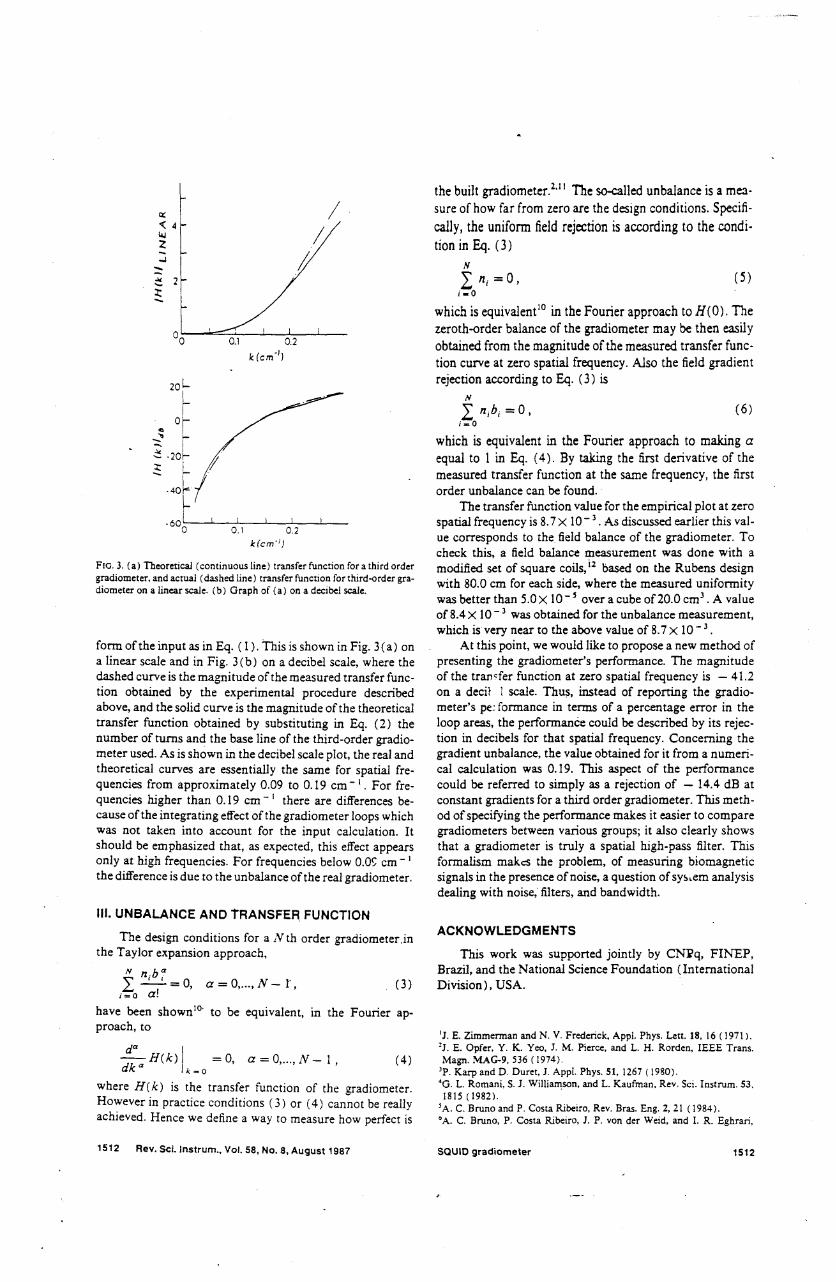
whieh is equivaleneo in the Fourier approaeh to E(O). The

zeroth-order balance af the gradiometer may be then easily

obtained from the magnitude of the measured transfer fune

tion curve at zero spatial frequeney. Also the field gradientrejeetion according to Eq. (3) is

(6)

(5)

N

Inibi =0,i_O

whieh is equivalent in the Fourier approaeh to making aequal to 1 in Eq. (4). By taking the first derivative af themeasured transfer function at the same frequency, the firstorder unbalance can be found.

The transfer function value for the empirica1 plot at zerospatial frequency is 8.7 X 10- 3 • As discussed earlier this value corresponds to the field balance of the gradiometer. Tocheck this, a field balance measurement was done with a

modified set af square coils, i2 based on the Rubens designwith 80.0 cm for each side, where the measured uniformitywas better than 5.0 X 10-, over a cube of20.0 cm3 . A valueof 8.4 X 10- 3 was obtained for the unbalance measurement,which isvery near to the above value of 8.7 X 10 - 3 •

At this point, we would Iike to propose a new method ofpresenting the gradiometer's performance. The magnitudeof the transfer function at zero spatial frequency is - 41.2on a decit 1 scale. Thus, instead of reporting the gradiometer's pe: formance in terms of a percentage error in theIoop areas, the performance could be described by its rejection in decibeIs for that spatial frequency. Concerning thegradient unbaIance, the value obtained for it from a numerical ca1cuIation was 0.19. This aspect of the performancecould be referred to simpIy as a rejection of - 14.4 dB atconstant gradients for a third order gradiometer. This method of specifying the performance makes it easier to comparegradiometers between various groups; it also c1early showsthat a gradiometer is truIy a spatial high-pass fiIter. Thisformalism makcS the problem, of measuring biomagneticsignaIs in the presence ofnoise, a question ofsY!>LemanaIysisdealing wíth noise, filters, and bandwidth.

the built gradiometer.2,ll The so-called unbalanee is a mea

sure af how far from zero are the design eonditions. Speeifi

cally, the uniform fie1d rejection is according to the condi·

tion in Eq. (3)N

L ni =0,i.O

0.2

k(cm·')

1 I 1

0.1 0.2

k(cm'lj

-I--~ 2J:

form ofthe input as in Eq. (1). This is shown in Fig. 3(a) ona linear scale and in Fig. 3(b) on a decibeI scale, where thedashed curve is the magnitude of the measured transfer functíon obtained by the experimental procedure describedabove, and the soIid curve is the magnitude ofthe theoretica1transfer function obtained by substituting in Eq. (2) thenumber of turns and the base line of the third-order gradiometer used. As is shown in the decibe1 sca1e plot, the real andtheoretica1 curves are essential1y the same for spatial frequencies from approximate1y 0.09 to 0.19 cm - I . For frequencies higher than 0.19 em - I there are differences because ofthe integrating effect ofthe gradiometer Ioops whichwas not taken into account for the input calcu1ation. Itshould be emphasized that, as expected, this effect appearsonly at high frequencies. For frequencies below O.Oçcm - Ithe difference is due to the unbalance ofthe real gradiometer.

FIG. 3. (a) TheoreticaJ (eontinuous line) transfer funetion for a third order

gradiometer, and aetuaJ (dashed line) transfer funetion for third-order gradiometer on a linear scale. (b) Graph of (a) on a decibel scale.

11I.UNBALANCE ANO TRANSFER FUNCTION

This work was supported jointIy by CNi'q, FlNEP,Brazil, and the National Science Foundation (lnternationalDivision), USA.

ACKNOWLEOGMENTS

(3)a = O,... , N - r,

The design conditions for a Nth order gradiometer.inthe Taylor expansion approach,

N ba" ni iL --=0,

i=O a!

(4)

have been shownIO' to be equiva1ent, in the Fourier approach, to

da I--H(k) =0, a = O,oo.,N- I,dk a k =0

where H(k) is the transfer function of the gradiometer.However in practice conditions (3) or (4) cannot be reallyachieved. Hence we define a way to measure how perfect is

'I, E. Zimmerman and N. Y. Frederiek, Appl. Phys. Leu. 18. 16 (1971).'I. E. Opfer, Y. K. Yeo, I. M. Pierce, and L. H. Rorden, IEEE Trans.Magn. MAG-9. 536 (1974).

lp. Karp and D. Duret, I. Appl. Phys. 51,1267 (1980).4G. L. Romani, S. J. Williamson, and L. Kaufman. Rev. Sei. Instrum. 53.

1815 (1982).

5 A. C. Bruno and P. Costa Ribeiro. Rev. Bras. Eng. 2, 21 (1984)."A. C. Bruno, P. Costa Ribeiro, J. P. von der Weid, and 1. R. Eghrari.

1512 Rev. Sei. Instrum., Vol. 58, No. 8, August 1987 saUID gradiometer 1512

BiomagnclISm: ,~pp!ications and Theory. edíted by H. Weínberg. G.Slrmnk. and T. Katíla (Pergamon. New York. lC)84). p. 67

'M. Sehwanz and L. Shaw. Signa! Processing (MeGraw-Hill. Tokyo.1975).

'T. Chen, One Dimensiona! Digital Signal Processing (Dekker, New York,1979).

·A. C. Bruno and P CO\IJ Ribeiro. Cryogenic\ 23. ,24 (198,)I"A. C. Bruno. P. CO\IJ Rlhclro. J. P \on dn We;J. and O G. Symko. J

Appl. Phy>. 59. 2584 ( 1(86)

li], Vrba. A. A. Fife. M. B Burbank. H. Weinberg. and P A. Bnckell. CanoJ. Phys. 60,1060 (1982)

I~R. Merrit, C. Purcell. and G. Stroink. Rev. Sei. In"rum. 54. 879 (1983).

1513 Rev. Sei. Instrum., Vol. 58, No. 8, August 1987 saUID gradiometer 1513

ANEXO 5

(Received 17 Apri1I987; accepted for publication 16 November 1987)

I!j

f

jj

I.•,III1

I!i

(3 )

(4)

(:2)

2820

a =O,I, ...••V - 1,

''?' 1988 American Instltute 01 Pl1YSlcs

N b12

~ n -' -O'-~a I a! - ,

where R ~121 (zo) is the derivative of order a ofthe field B, (:)at zO' Substituting (2) in (I), considering only spatial de·pendence. the flux through the set of coils can be expressed interms of the field and its derivatives at the first coil:

where bi = Z, ~ Zo is the distance between the ith cai] andthe lower one. The gradiometer parameters are obtained b:solving system (4). Frorn visual inspectiGlnone can see cha((4) is a system that has N equations and 2N -I- I unknowns.1n order to solve it. /li + 1 unknowns must be transformed ;npa.amcters of,he sY5tem. According tu the un~.J:uwu~ ~~~~~~formed. two kinds of solutions will arise. For instance. suppose that the ,'ib,'s (b\,b1 = 2b\•...,by = ;Vb\) and onen, (no) are chosen. In this case the solution for the systemwill be given by the Newton binomiaHormula4;

coil, B, (i) is the normal component ofthe magnetic field atthe coiU, N + I is the number of coils, and 1(t) is the timedependence of the field. Expanding RI (z) in Taylor seriesaround the origin (zo) yields

z R(12)(Z)

B, (z) = I ' o (z - ZO)12,12=0 a!

This solution leads to the conventional gradiometer designoHowever, if the"V + 1n; 's are chosen, one will have :he firstequation solved, so one more unknown must be chosen. Suppose that the one chosen is the total length of the gradiometer h.v. As was shown,' this is the most geneIl1 choice forsolving system (4), and willlead to solutions wI\ere the b, 'sare not multiples of the smaller ones.

The gradiometer output signal will be proportional tothe field deriva tive only for distant signal sources. Only if thesource is at a distance much Jarger than the gradiometertotallength will series (3 ) converge. 6

Todesign anN th-order gradiometer, the first N terms af(J) must be made equal to zero to reject the noise. Then, chefollowing system of equations is obtainedJ;

(1)

,002, ·8979/88/082820-04$02.40J. Appl. Pl1ys. 63 (5l, ,5 April 19882820

( N \dJ(Zo.t) = A I n,B" (:,) )1(1),\~-o \

where A is the area of coib. n i is the oumber of tu.rI\~of each,

A. C. Bruno and P. Costa RibeiroDepanamenlo de Fuica. Ponllficia Universidade Católica do Rio de Janeiro. CP. 38071.22453 Rio de Janeiro RJ. Brasil

11.REVIEW ON THE OESIGN OF GRAOIOMETERS

The equation that deserihes the total flux tfJ(zo,t)

through a set of coils axialJy positioned along the z axis, thefirst coil being at Z()J C3.Il be sUted as

A review of the traditional method for designing gradiometers is made. A nonrecursive digitalfilter modeI for the gradiometer is presented, givlng a new set of parameters for thegradiometer identification. Some designs are analyzed using the proposed set. As an example, atrue differentiator is designed to be used as the SQUID input coil. It is shown that theditferentiator has the same noise rejection as the conventlonal gradiometer but provides moresignal sensitivity.

ln the late sixties, the appearance ofthe SQUID was themost important fact for the deveIoprnent of biornagneticmeasurernents, which are being made in several research institutes and hospitaIs. The SQUID is usual1y coupled to asuperconducting circuit ealled :l flux transformer. It consistsof a set of coils for field sensing. connected ín series with asolenoid placed inside the SQU1D body. When a magneticfield Ís applied to the coils, a persistem current appears in thecircuito producing a magnetic flux inside the SQUID.

Usually the measurernents are made in environrnemsthat have magnetic interference from power lines, motors,eIevators, etc. These fields have magnitudes that surpass biomagnetic fields by a factor of at least 10000. Some filteringprocedure must be used in order to remove the unwantednoise. A possible solution is to place the patient and instrumem uf measurement inside a magnetically shieldedchamber. Another technique is to use the set of coils coupledto the SQUID, in a gradiometric configuration, I to make aspatial discrimination berween signal and noise. This occursbec:luse the noise source is very far from the gradiometer andthe weak source is placed elose to it. The monotonic spatialdecay of the noise can be modeled by low-order terms of aTaylor series expansion. As the gradiorneter ·:ancels the firstderivatives the far source field will not be detected.

Thls paper makes a re.•.iew of the gradicmeter analysis:.lnd design processo It is a mere fCrTIul:l7ij ge:-:'::":llap[Jr0achof a formalism than introduced previously,1 showing thatthe gradiometer ís a digital spatial filter. The gradiometerdesign is discussed using convencional filter analysis parameters. These parameters can be used to deseribe the gradiometer design instead of its geometrical description. Finally.using this formalism, first- and second-order àiíferentiatorsare designed to be used as the SQUID input coiL The durerentiators will theoretical1y have the same noise rejection buta better signal sensirivity.

I. INTRODUCTION

Digital filter design approach for SQUID gradiometers

'i-

; -~ r.

IV. GRADIOMETER DESIGN WITH A FIL TERINGTECHNIQUE

It can be seen below how the traditional gradiometerconfigur:ltlon anses when a digital tilter design procedure isused for a high-pass transfer fum:tion. One condition charguar::lntees che effeetivene;s Cor a smoorh high-pass tilter is

Substitution of (9) In (8) willle3d to

Ht (s) = r\, (10)

This will ensure a maximally fiat stop-band cransfer functionfulfilling conditíon (7) .

The gradiometer realization of (10) ean be made byusing one of the transforms from the Laplace space to thedigital space. It consists in replacing the differential equation

related to Hg (5) with a diiference equation.IO This can bedone by making the following substitution of variables:

5=I-z-', (lI)

where z is the variable in the digital domain (z = e 1 !<.A. , ).

Then, H(z) can be written as

H(z) = (l-z-I).". (l2)

For i'í= I,

H(z) = l_z-I; ,(13)

for N = 2,

H(z)=l-2z-I+z-:; (14)

for N= 3,

H(z) = I - 3z-1 + 3z-: - Z-3; (15)

for i'í = 4.

H(z) = I - 4z-1 + 61-1 - 4z-3 + z-~; (16)

and 50 on.

10e gradíometer earresponds to a direct canonic realization of the above cransfer functíon.7 where che eanoníe

means nurnber of base lines equal to che cr3nsfer functionorder. For instance. transfer funcrion (15) shows char "I"stands for the tirst coil with one Cun:..• - 3z- I" means chat

after one l, there is a coil witb chree turns in the opposicedirection, "3z-2" means that after two l, there is a coil withthree tums in the same direction as the tirst one, and finally.. - z- 3 •• means that after three Â, from the begínníng of Chegradiometer there IS a cai! with one tum in che opposite direction. The magnitude of lhe cransfer function (12) expressed in decibels is

!HCz)i = 20 Iog[2"'sins(U,I2)]. (17)

Usually, the magnitude or the niter transfer functlonplot is divided in three parts: StOpbando rransiClon bando andpass bando The stop band is usually evaluared by che maximum rejection given by the tilter. In our case. this is equivalem to rhe gradiometer balance reached. II The cransitionband is measured in terrns of roJloff per decade of freq ueneyand the pass band by the cutoff frequency and maxim umgain. If rhe gradiometer is balanced up to 10-4, che maximum rejection achieved will bc - 80 dB at K = O. Assuming kÀ.,12.( 1 in the transition band, one can have

rollo6' =, ::-20 N dB/decade. ( 18)

The cuto6' frequency can be expressed as

k< = (2/À,)sin-I[(0.707)I/N]. (19)

Finally, the maximum gain is

H(k,..) = 20 log(2N), (20)

where k .••= lTI À,,7 as the gradiometer is a digital spatialfilter.

(7)

(8)

(9)

(6).v

H(k) = A )' nie -JÂ>À. ••,.0

Hg(s) = 1-iIHo(s).

If denormalized. Hb (s) can be written as

Hb (s) = 1/( 1 -r").

d"" Hlk)---- = O. a = O.l, ... _V - 1,

'íka k~O

where IV is the order af Lhefilter. Equation (7) shows thatthe stop-band fiatness of a hign-pass transfer function inereases when rhe order ofthe tilter increases.

A me~hod for synchesizing a digital tilter is to tind theproper transfer functIon. H(s), in Laplace space using thec1assical filter theory. 10e analog design is then rransformedon a digital realization. A possible design having pass-bandfiat is k:nown as Butterwonh.. 9 However, condition (7) requires that the stop-band be fia!. Neverthel~ the Butterworth polynomial Hb (s) can be used to make the desiredtransfer function Hg (s) in the following way:

k being the spatial frequency.In thar approach signal and noise will be described by

the spatial Fourier spectra. In doing so, the noise will have aspectrum with low frequencies and the signal wilI be represented by a much wider spectrum.8 Using the C:igiral filtermodeling, a gradiomerer spatial transfer function could bedesigned for each noise and signal specification.

}.-< ill. DIGITAL FIL TER MODELlNG

kt1 As was said elsewhere.: the gradiometer is a device thatsamPles the signal and noise at discrete points in space. that

;,\.cOrrespond to the coil positions; thus. it is a spatial digital••sampler. 10e sampling period À, is given by the minimum

~distance between the coils. Moreover. the gradiometer

~makes a weighred sum of the input field sampled sequence.

_ .~~ The weighting factors depend on the area of each coil. 10e

iIr.' gt3diom,,,," a non'"u"i" digiul 'palial filt."..Th~ ""'~ .• be ilIustrated with the following arguments: the basic digital·L.: tilter elements are the unit delav, the adder, and the multi-

~-J ~

~~. plier.7 Therefore. digital filters are collections af intercon-

i, nected unir delays. adders, and multipliers. A gradiomerer

.,. bas in its hardware the elements that correspond to tbose.. )

.J7 three basic elements of the digital filter theory. The sampling.~~ period À, corresponds to the unit delay. The fact that all the'r coils are wound in series corresponds to the adder. Finally,t the area of each coí] corresponds to the multiplier. AlI the

fonnalism already developed for digital filters can then beused to analyze and design gradiometers. Assuming a syrnmetric deslgn (all eoils w1th the sarne area), the gradiometerspatial transfer function H(k) can be obtained by taking thediscrete Fourier transform of the sequeJ;1cethat representsthe number of rums of each coil"':

2821 J. Acpl. Phys .• Vai. 63, No. 8. 15 Apnl1988 A. C. 8r1Jno and P C. RibeirO 2821

TABLE I Filter paramelers to ""I- (sce Ref. 12). second· (aI (scc Rei ~ O ~,-------

IJ 1. second- (b) (~Ref. 14l. and thlrd· (sce Ref. IS) order gradlome!ers, C' =- (I' !

i,-

t •• :I~ --IGradiomtler

RollolfIe.Ie_H(Ie_) l ---:-dcsigns (dB/decade)(em-I)(em-I)(dB)::l«fint

- 200.130.316..I.~

sccond (a)

-400.40.6212":t

SCl:ond (b)

-400.620.9812third

-600.40.3718

V. DES/GN OF A DIGITAL SPATIAL DIFFEREN71ATOR

Another method for designing a digital fiIter is to abtainthe filter coefficients from the Fourier series representation.as shown below. The transfer function of a nonrecursive di

gital weighted sampler iS',b

2822

(261.

1.005

A. C. Bruno at1d P. C. RibeIro

and

Ir. = -2( -1)"!(nÃ.,)=]. for n = -N to N. (27)

The transfer function of tbis second-order spatial differentiator using the same Hamming window with N = 10 (20coils) and a conventional second-order gradiometer with thesame sampling period, as shown in Fig. 2. A1so shown in Fig.2 is the normalized magnitude of the Fourier transfonnsIB(k) I ofa current and magnetic dipole placed, respectively,at 1, and 50;., from the position of the first coil. As can beseen, the ditferentiator will provide a better signal-to-noiseratio. since it has more sensitiviry for high-frequency tennsofthe Fourier spectrum which eonstitutes the main signal ofinterest.

The direct truncation of this antisymmetric sequencewill result in a spatial filter with a quite oscillatory transferfunction. The ripples can be vinual1y eliminated by using awindowing technique to truncate the sequence of the spatialfilter coefficients (coil area). For instance. the Hammingwindow is given by the following expression 17;

tu. = 0.54 + 0.46 cos (nr.IN), for n = O toNo (25)

Windov-ing consists of multiplying the window factors tu.with the coefficients h•. The new fiIter coefficients will be asmooth1y decreasing.series. Such a ditferentiator would havea neariy conical shape. since successive coils wouId have lessareu.

As shown in Fig. I, the transfer function for a digitalditl'erentiator (continuous tine), using N = 3 (six coiIs) anda Hamming window. is quite satisfactory when compared tothe one of an ideal differentiator (dotted tine). It can aiso benoticed in Fig. 1 that the firsr-order gradiometer (dash..,jotted line) acts for low frequencies as a differentiator. As noisesources have only low-frequency Fourier components, a differentiator has the same rejection for them as a first-ordergradiometer wirh the same sampling period. Moreover, it isimportam [O stress that with lhe ditferentiator. not only thenoise but rbe near source field will be differentiated.

If more noise rejection is required. a second-order ditl'erenciator can be d~igned in the saroe way. In doing so, th •..filter coefficients (coils' areas) will be the following:

FIG. 1.Transfer functions m K space (ko = 17"/ À., l ofan ideal differenlialor

(doned line " a digital realization of il (conlinuous line) with N = 3 (six

coils). and a conventional tinl-order gradiometer (dash-doned line) Wllh

lhe same sampling periad. (a) The dilferenliator and (b) the gradiometer

are represenled in the inseto

(21)

(22)

(24a)

(24b)for n = - N to N,

J. AppL Phys .• VoL 63, No. 8.15 Apnl 1988

=

~H(k) = I h.e-i<""-'.

,,- - :o

( - 1)"nÀ.,

andh. =Oforn =0.

The filter coefficient h. should in general be considered thegradiometer Ioop areas and ean be obtained by taking themverse Fourier transfonn ofHlk);

À. [/~'h. = -' H(k)ejk",,-, dk.

2:T - r/ÁJ

As anexarople. we d~ribe the design or a digital differentiator. The differentiation corresponds. in the frequencydomain. to the multiplication ofthe Fouriertransfonn oftheinput by the factor jk. The characteristic of an ide-al digitaldifferentiator is given by

H(k)=jk, for -trll,<k<trll,. (23)

The filter coefficients h" can be obtained substituting (23) in(22), and truncating the resu1ting scries:

1 [")''h" =-' (jk)ep.;.'dk,211' - ,/"ls

2822

Table I shows the set of parameters of first-, second-.and third-order gradiometers. The gradiometer maximum

rejectioo does not depend 00 the desigri, 50 it is not listed in

the table. The maximum gain ofthe pass band and the rolIolfper decade of frequency depeods only on the order of the

gradiometer. As the order increases both parameters willincrease. 1n doing 50, the transfer function w1l1 becomesharper because the rol1otl'will increase. The maximum gainwill be at ditl'erent spatial frequencies for gradiometers of thesame order with different baselines. The frequency for maximum gain depends only on the baseline, i.e., a large baselinewilllead to a small k",. Finally, the cutotl'frequency dependson the order and baseline. If the arder increases kc will increase: however, if the baseline increases kc will decrease.

The shape of the spatiã.J frequency spectrum depends anthe source position. For instance, a superficial brain sourcewill have a spectrum wider than a heart source.8 Hence, alarge kc (short baseline) shall be used to detect a brainsource. However, the gradiometer design will a1ways be atradeotfbetween its H(k",), rollotf, and kc.

r~'Tk~:';'i;~'1"-:~7~~t!"--'.~~""".-."

VI. CONCLUSION

ACKNOWLEDGMENTS

This work was partially supporred by FlNEP, CAPES.and CNPq.

'J. E. Zimmerman and N. V. Fredericlc. Appl. Pbys. ~l. 19. 16 (1971).

2A. C. Bruno, P. Costa Ribeiro. 1. P. von der Wcid. and I. R. Eghran. inBiomaglletism: ApplicallollS aNi Theory, edited by H. Wemberg. G.Stroinlc. and T. K.atiLa (Pergamon. New Yorlc. 1984). p. 67.

Jp. lúrp and D. DureI. J. AppL Phys. SI. 1167 (1980).~. L. Romani. S. 1. Wil1iam50n. ma L. Kaufman. Rev. Sei. Uulrum. 53.

1815 (l982).

IA, C. Bruno aod P COSta Ribeiro. CryogeniC3 23, 346 ( 1983).

·A. C. Bruno and P. Costa Ribeiro. Jl ev Bras. Eng. 2. 21 (1984).

'A. Anloniou. Digiral Fi/ter;, .~lIQI)'$1S and Design (McGraw-Hill. ~e';l,'York. 1979).

IA. C. Bruno. P. Costa Ribeiro. 1. P. von der Wetd. and O. G. Symko. J.Appl. Phys. 59. 2584 (1986).

"J. K. SkwtrZynsh Desigll Tireory and Data /or Elecr1'01IlcFilters (V anNosuand. London. 1965).

10A. v. Oppenheim and R. W. Schafer. Digital Signal Processing (Prentl~.Hall. New Je~y. 1975).

IIP. Costa RibeIro. A. C. Bruno. C. C. Paulsen. and O. G. Symko. to RevSei. lnslrum. 58. 1510 (1987)

I:M. Saannen. P Siltanen. P. 1. K.arp. and T. E. K.1tila. Ann. Oin. R~. 10.I (1978).

IJS. Barbanera. P Careli. R. FeruCl. R. L:onl. l. ~odena. and G. L. Ro

mani.IEEE Trans. ~agn. ~AG-7. 849 (19811."S. l. William50n. D. Brenner. and L. K.aufman. AI? Conf ?roc. ~. 1(){í

( 1978).

"J. Vrba. A. A. Fife.~. B. Burbak.. H. Wetnberg. and P. A. Bnc"etl. Can.J. Phys. 60. 1(0) ( 1982).

16M. Schwanz and L. Shaw. Si~al Processlflg (McGraw·H.ill. Tokyo.1975).

"c. T. Chen. 01le Dime~ional Digital Sigllal Processillg (Marcel Dekker.New York. 1979).

38

a7

5.8 ~III

10o

O

I'a~

[~,::l<C \

~~ \~ t \

\

A review on the traditional gradiometer design processwas made. A complete equivalence af a gradiometer and anonrecursive digital spatial filter was shown. providing anew method for synthesizing the convencional gradiometerconfiguracions. In addition to that. instead af a simple geometric descripcion. a set of parameters based on the filtertheory was proposed as a new way of reporring the gradiometer designoFinal1y, using digital design techniques, digitalspatial differentiators are designed and the transfer function

is compared to the one af conventional gradiometer.s.

05

lHo

F1G. 2. Transfer functions in K space (kn = :r1À.,) af a sccand-order gra

diometer (conunuous line) and a secand-order di/ferenlÍalar (doned line).

W1th lhe same >.lmpling penad. Normalized magnitudes af the Faurier

transforms of a near current dipole (dashed line) and far magnetic dipole(dash-<ioued line) sources.

'r·

~.

-

2823 J. Appl. Pt1ys .• VaI. 63. No. 8.15 Apnl19S8 A. C. Bruno and P C. Ribetro 2823

ANEXO 6

DI~cretespatial fllterlng with saUID gradiometers In blomagnetismA. C. Bruno, P. Costa Ribeiro, and J. P. von der Weid

Department of Physies, Pontificia Universidade Cato/ica, Rio de Janeiro. Brazil

O. G. SymkoDepartment of Physics. University of Utah. Sa/t Lake City, Utah 84112

(Received 4 Apri11985; accepted for publication 6 December 1985)

First-, second-, and third-order gradiometers used in detecting biomagnetic signals are analyzedas spatial filters. Their transfer functions independent of the source to be measured are presentedand both the magnitude and phase characteristics of the transfer functions are analyzed. Thedistortion introduced by the gradiometer can be estimated from these characteristics. In order totreat the signal in that approach, the spati~ Fourier transform of a magnetic signal produced by acurrent dipole at a given distance is discussed.

INTROOUCTION

For a number of years SQUID magnetic sensorsl havebeen used in biomagnetism research and have been instrumental in significant achievements in the fieId. Usuaily thesignal is coupled to the sensor by a fiux transformer whichhas the detection coil in a gradiometer configuration for spatial discrimination between signal and noise.2 This techniqueis also used in other fieIds of research involved in the detec

tion of reIativeIy weak magnetic fieIds, the monopole searchbeing one of them. 3.4

A gradiometer can be basicaily described as an array ofcoils, the lowest one, called the "pick-up" coil or "facelcop, ,,5 being primarily sensitive to the hear source of signaland the others acting as "compensating coils" to eIiminatethe far sources of noise. Such a simplification has to be abandoned when a quantitative result is needed, as in the case forthe Iocalization ofbrain sources; the influence ofth.e "compensating coils" on the signal should then be taken into account.6

Usually each Iaboratory working on biomagnetism hasits own gradiometer, des(.ribed as being offirst, 7 second,8.9 orthird order10•J 1 with given distances between coils, numberof turns, and area of each coil. The choice for the actual

values of these parameters has been rather qualitativeIy dictacted by the kind oflocal background noise and signal to bemeasured. Usually in a comparison of coils, the assessment isbased 01' iloise leveI achieved by these diíferent systems and

is presented as a value in IT/ fHZ for the equivalent fieIdspectral density or power spectrum of the noise in the pickup coil ..

With such an approach it is diflicult to know the exactnoise rejection of each system (the actual background noiseis not known), thus ma,king it diflicult to compare them.Also, ifthe source is not just a current dipole (as is the case ofthe heart), the signal spatial dependence is not known. Suchshortcomings have been partialIy overcome by the approachof Wiksw05 and Storey.12 They used the reciprocity principIe to make a comparison between diíferent gradiometer designs for noise rejection in the presence of magnetic dipolesources only. The sensitivity of various gradiometer configurations to only current dipole sources has also been calculated.5

We present a more general approachl3 to this problernby describing analyticaily the gradiometer in terms of itstransfer function irrespective of the kinds of signal or noise.Our approach is such that gradiometers are high-pass discrete spatial filters whose transfer function enables a comparison to be made between the different gradiometer configurations. Such transfer functions will help to select thebest design for'a given signal and noise, as weil as to determine the eft"ectof the "compensating coUs" on the signal.

The fundamental idea in the use of gradiometers to discriminate the signal from the noise is that in a given region ofspace, the spatial magnetic field dependence can be fitted bya polynomial (Taylor series). Far sources (noise in our applications) are fitted to only one to three terms of the poIynomial, sincejust the fieId and its first derivatives are predominant, whi1e near sources (the signal in our case) will,'equirea larger number of terms. A gradiometer makes the spatialdiscrimination by canceling the first terms of the poIynomial,

Althougb it is not customary procedure, the monotonicmagnetic fieId spatial deper.dence can be fittedjust as weil bya Fourier expansion. 1n such an approach, spatial discrimination is reached by using the fact that a distant source wiilhave low frequency components ofitsspatia/ frequency spectrum, whi1e near sources wiil have Iow and high frequencycomponents. The spatial discrimination is then achieved byusing a spatial high-pass filter.

The use of spatial filters is weil known in other fieIds,such as optics14 or tomography, 15 and can be instructive anduseful to apply to magnetic fieId studies in biophysics. This isthe goal of this paper. The gradiometer is presented as anonrecursive spatial filter with its own transfer function;then this approach is compared to the conventional Taylorseries approach. Fina11y, the spatial Fourier transform of thesignal is considered, to show how the various gradiometers(Le., filters) will respond to it.

THE GRADIOMETER SENSOR: A TAYlOR SERIESAPPROACH

The general confi~ation of an N th order gradiometeris shown in Fig. 1. It consists of an array of N + I coilsconnected in series, each with ni turns, and separated by the

'.

2584 J. AppL Phys. 59 (7), 1 April198S oo21-8979/8S/072584-06$02.40

r

@) 1985 American Institute 01Physics 2584

that characterize such a gradiometer ax:ederived by cansidering the total flux iP(zo,t) applied to the array. with thelowest coil at Zo from the source,

~ ----nj ~ - - - --

,.-,'---. - - - - - - - ,n "--L.-/ - - - I

3 I I

nz ~ - - - - - -

I

n, ~----J l,bZb b,- - -1- __

no - - -

bi

=A (i n,B(z,) \,.(t) ,l_O f ( 1 )

FI G. 1. Gradiomcter af N th arder.

distance bj from the lowest cail. For simplicity, we cansider

the case where they alI have the same areaA. The equationsl

where B(Zi ) is the magnetic field component normal to theplane of the cai!, Zi is the distance from the ith cai! to the

origin, andg(t) is the time dependence ofthe flux, expressed

separately since biomagnetic Íle1dsare quasistatic.

Expanding B(z) in a Taylor series about the position Zo

of the lowest coi1 and letting bj = Zi - zo, Eq. (1) can bewritten as

~!lJW (zo,t) = A{noB(zo) + n1 [B(zo) + B (l)(zo)b1 + B (2l(zo)(b f /2) + ...]

+n2[B(zo) +B(I)(zo)b2+B(21(zo)(b~/2) + ...] + ...}g(t).

This can be arranged in matrix form as

(2)

no + nl + n2 + ...n1bl + n2b2 + ...

b~ b~n1-+n2-+ ..·

2 2

oB(zo)

B(l)(zo)

B (2)(zo)g(t). (3)

o

Such conditions are fulfilied by alI existent gradiometers,even by the so-called asymmetric ones that use differentareas for the sets of coils, and where ni is not J;~ted to be aninteger.

The above diagonal matrix expresses the eífects of the arrayof coils on the field and its derivatives B (I),.B(2) , ••• at zo, thepick-up coil position. A gradiometer of N th order wi11resultwhen thefirst N diagonal terms are canceled, that is imposing the condition,16

!V b a .I ni-' = 0, a = O,... ,N - 1.i-O a!(4)

r

This procedure defines a new set ofnumbersy", from the setof numbers x'" which correspond to the sampled values atconstant intervals. The weighting factors hi depend on thefilter.

The discrete Fourier transform (DFr) of the signal(see for example Ref. 17) at some instant oftime can then beexpressed as

(6)

where k is the wave number and Às is the distance betweentwo successiv- sampling points.

For our case of the gradiometer, assume that the distances bj can be expressed as multiples of Às,

or considering the digital nature ofthe detection scheme,

!VI (z •••) = I nj~(z", + bj),;~o

where 13. has integer values and Às are the maximum common divisors of alI the bi• The signal detected by the gradiometer at position zm over ali its space will be

(8)

(7)

IVI...= I n,~", + "i ""'"o

THE GRADIOMETER SENSO R: 'A NONRECURslVEsPATIAL FILTER APPROACH

A gradiometer detects a continuous time signal, sampling it at discrete points in space bj which correspond to thecoils' positions. The net detected signal, at each instant oftime, is a weighted sum of all those sampled values. Thus itseems appropriate to use a digital mathematics fonnalismfor describing the gradiometer sensor.

In such an approach, the output of a so-called movingaverage or nonrecursive filter is generally expressed asl7

""

Y •••= I hix", - j'i=--ao

(5) where N + 1 is the number of coils, and ~(zm + bi)

= ~'"+ i is the magnetic flux at the ith coil at some instant of

2585 J. Appl. Phys., Vol. 59. No. 7, 1 April1986 Bruno et ai. 2585

I i ' i I ~. lt "Hlij.ll,·1

,.,

('

454 BIOMAGNET1SM '87

PLANAR GRADIOMETER INPUT SIGNAL JU:COVERY

USING A FOURlER TECHNIQUE

A.C. Bnmo, A. V. Guida and P. Cosia Ribeiro

Dep&NmerSo de Fw~ Pontifícia Univel"lidade Cai6lica do Rio de Janeiro

C.P. 38011,22453 Rio de Janeiro RJ, Bruil

(

(

1. INTRODUCTION

A greu technicaJ improvement in cndiometer constructioD has b~n obtained with thin film deposition

techniques (1, 2). These tecl1niques usual1y lead to planar designa. However, ~he output signaJ for thia kindof gndiometer wouJd be more difticult to interpret than the output of the commOD uiaJ ones (3). Tbe .patiaJdependence in the z diredion, perpendicular to the coi! plane, of & biom3il1etic sourte is monotonie, but theapatiaJ dependence in ~he eoil', plane, % and r dirediol1! &te usually noi monotonic. Thia means thú the signaJin ea.ch planv gra.diometer coil could be equalJy large. 10 other words, in & planar gra.diometer there ia not &pici-up coi! tha.t senses mosi of the aigna.l and the compenaa.ting coila rejeet noise. This, would m&lte it impoaibleto flnd a. IOlution to the invel'3e problem by simple inapeetioD of the output mea.suremenb eveD for .uch & simpleSOUlce as the curnnt dipole. However, it is a.lwa.yspossible to uae a. fttting routine with vvi&ble panmetel'3 once& mown aourte is expeded (t).

The objed of thi. papel' is to appty to plaou configun.tiol1l a.digital spa.tiaJ fiUer model previOUlltydevelopedfor &Xia.lgndiometers (5). This model will provide toola to overtome the problem of plaou gra.diometer outputsignal interpreta.tion, without m&king a.ny previOUl a.saumption &bout the tind of fleld lOurce.

2. RECOVERY METHOD

Tbe three maln e1ementa in a. S}'!iem approa.ch a.re the input, the output and the trarisfer fundion of theS)'Iiem. According to thia a.pproa.ch the gradiometer WI be aeen u a. nonrec:unive digita.l Ipa.tiallilter h&ving itsown tr&nafer fundioD. More apecifically it ca.n be seen as &movÍDg &veTaie filter. This kind of digitallllter s&mple=lthe .ignal to be me»ured wíth a. sampling perlod .À. &Ild then mues a. weighted sum of the sa.mpled lequencea.ccording to weighting factol"lh',. The CeJ1eraJeJCpl'ell8ionfor the traosfer funetion H,(k) of this IIlter is (6):

CIO

H,(á) = L h.4e-;IriÃ.,i::-Q)

(1)

The equivalence between a. moVÍDg a.ven.ge lUteI' in .pa.ce and a.n a.xial gra.diometer ia pouible (5) becauaethe gra.diometer ~ -aamples" the ma.gnetic field intenaities u dilferent coil positiona, mUing a. weighted auma.ccording to the number of tuma in ea.cb coil (if a. symmetric design ia ~naidered). Thua, a.ccordin~ to (1) thegradiometer spatial traDlÍer fundiDo H(k) WI be expressed u:

H-I

H(á) = A L ",e-;Itíl,i=O

(2)

where k ia the apatia! !requency, A ls the &rei. of the coiJa, N ia the nUr:lber of colls, '" ia the number of turnsof each coll a.nd I ia the baae Une. lt ia Ulumed tha.t gra.diometer eoil'. surfa.ce ia ao small thú the 6eld hu& uDÍfonn di!tribution over it. Abo H(k) cao be mea.rured experlmenta.l!y with a. procedure alrea.dy developed(1). Substituting tbe \lllual values·for the ft;'S a.nd I.H(i) will h&ve a. higb pa.ss .hape. To complete the S)'Item&pproach, the çadiometer input can be deftned as the field seen by the flrst.çadiometer coil b(z) a.nd the OlItputia deftned as the fiux .eenby the whole gndiometer '(I).

10 the case of planar gn.diometers it ia atra.ightfowvd to apply the digital lUter modeling u b.r as Unevgra.diometers a.re concemed (3). Theaampling DOWoecurs in one direetion of the gra.diometer pla.ne, for insta.ncethe z direetlon. The aame expression for H(k) can be U!ed to show the effect of the gra.diometer over the signalto be meuured.

~ in a.ny ay_tem, the reluion beiween the input b{z) and the output ;(z) in the frequeney domaJn eaa beapressed 11:

t(k):= H(k)B(á) (3)

\..~---------

. /

and for the seeond order three terma:

11 i '

I! !

(6)

(5)

455

2512.5

i.

'.'

oDistonce

-

-12.5

CX__ >c=J

••c:01C~

"'--

-25

BIOMAGNETlSM '87

b(:) = 21, J: B(k)eih di.

Fig. 2 - Output signaJ (dot·ted line) of a. Ilrst order lineargn.diometer as &function ofdistanee for &eurrent dipolesoutCe pla.ced &t &lfuta.oce Zo

below the gn.diometer. Recov·ered dipole field (continuo~line) Uling the Fourier metbod.

They have loopa of sma.ll a.rea A aepanted by a. lfutance I. To calculate the transfer ronction of the fint

order gndiometer, the summa.tion in Eq. 2 will ha.ve only two tenns:

H(i) =A[1-2e-;kl +e--;k2l]. (7)

To produce the output ,(%), the dipoles a.re positioned in the following way: the cumnt dipole ia pla.ced&t the : axis :o em below the gndiometer plane &lld i5 oriented in the , direetion; ."hile the ma.gnetic dipole iapla.ced ai the same pOIition but oriented ÍD.the_z direetion. Tben, the gn.diometer is di5pla.ced a.Iong the z a.xistrom -00 to +00 giving an output a.s a. fundion of:. The output of a. Ilnt order gn.diometer for a. eurrent dipolesource pla.ced &t 10 = 3em, ea.n be seen ai; Fig. 2 (dotted line) and i5 given by:

Fig. 1 - Schema.tie dn.."ing offir3t and second order linear

gn.dio meiers.

3. SIMULATION

AI. &Ilex.a.mple, simul6tiona of the l'l!Covery of the z component o'"the m&gDetic fte!ds genented by I. cumnta.nd ao magnetic dipole are done. The signals a.re detected by planar /Il'3t &Ildsecond order gndiometers &long the

% diredion (Set Fig. 1).

B(i} = +(i}fH(i). (4)

Since the output ftux of the gndiometer ~(:) can be measured, itlJ Fourier tr&nsform t(k} can be calculued.

H(k} C1Jl be calculued from Eq. 2, thua the input field b(:} C&lIbe found by tiling the inverse Fourier tnnsfonn

of B(k) u follows:

."here t{i) ia the Fourier tnnsform of the output /Iwc ;(%) and B(i) i5 the Fourier tnnsform of the input /Ieldb(%). ThUl tbe Fourier tnnJform "af b(%) ean be oMained by:

•

••

r

~. ;~'r~ 456 8JOMAGNETlSM '87

(8)

"here A = 1, b( %) Í3 given by the Biot·Sa~ Ia.w &nd 1= 2 em. The output is not symmetric in relation to the

origin due to the choice of tuing the % = O position when thegn.diometer'a firat coU 11 a.t the origino

A Fourier tnnsform ia a.pplied to the output ,(%) &nd the reault divide<! by H(k). The invel'1e Fourier

transform of the division Call ~ be aten a.t Fig. 2 (continuoU! line) which ia the well known cun-ent dipole

pattem. The difi'erence between the l'!covered nJues anó the aduaJ eummt dipole field can be made li.! smaJI as

we "ant, depending only on the numerica.! premion used for the Fourier ea.!cul&tion.

Fig. 31. &nd 3b mpeetively ahowa the isovaJue contour mapa of the output of a.'fint a.nd sl'~ond order planar

gra.diometera over ao grid of 6 x 6 points, ea.ch one sepa.ra.ted by the gra.diometer ba.seline (I), for a current dipoleaourte. The vaJues of Zo &nd I were the aame as before. To recover the dipole lield vaJues in ea.ch position of the

grid, the Fourier procedure explained above ahould be used for eacl1 grid line. At Fig. 3c is displayed the iso/leldlines oi the recovel'!d field.

-

c

• c •

•

b

• b •

\ ;" - .,

• a •

a

Fig. 3 - lsovaJue contour map of the output of a. firat (a) and seeond (b) order linear gradiometer for a currentdipole souree pll.ce<! &t &distance zo below the mea.suring plane and oriented in the 1direction. Recovered isofieldcontoun using the Fourier technique (c).

Saroe u in Fig. 3, but using a magnetic dipole as souree, isovaJue tontour mapa of the output oi the fint

&nd seeond order planar gn.diometera an abown in Fig . .(&and Fig . .(b reapeetively. The output oi the a.Igorithm

ia diapla.yed in Fig . .(c.

Fig . .( - IaovaJue tontour map of the output of a firat (a) and second (b) order linear gradiometer for a ma.gneticdip ole aouree pla.ced a.t a.distance zo below the measuring plane and oriented in the z direction. Recavered iaolieldcontoun uaing the Fourier technique (e).

;. (

--,BIOMAGNETISM '87 457

, ,: I

(9)

4. CONCLUSlON

ln order to implemeot the &Jgorithm, leme p~tioDll IDUJt be túen to UlIure from •. oummcaJ poim o(view, I. weU behl.ved eaJcuJa.tion. TheoretlaJJy H(O) = O, tbe gndiometer'a &reu lfere made aligbtJy di!'erent toI.void division by tero in Eq .•• lfitb HrO) ha.ving the vaJue of 0.001. The integral limita of the Founer in~

In spa.ce (dired) and in ~uency (lnvem) Wert w-efully chosen to eever I. finite atu. OVerthe lntegntion a.xiJ(8). The vaJues used in the examples were -30 to +30 em in apa.ce and -3 to 3 em -I in !requency. Coneerningpra.dica.l meaaurtmenta, when the output &llalytical expreesion ia not 3.V1.ilableas in Eq. 8, the aJgorithm predaionwouid be I. functioD of the number of output meuurementa tlien, the dist&llus betw~n them II1d, of eoune, the

experimentaJ eml'!. In pmioua ca.lcuJations, a negiigeably amaJJ &reI hu been U81·:ned; thU3 the two aamplingpointa loca.ted at O and I, eorrespond to the eenter oi tbe gra.diometer eoilJ. A poaible ny" to t&h into &ecount

a 6nlte &re1 eJreei, ia to eonsider the rtctanguJat aha.pe a.t FIg. 1. !bis ean be done by U!ing many mo~ wnpfing

pointa, aasuming a new ~. much .maller th&n I. This wli be equivaJent to aubdividing the LlU into •• l&rge

DUmber orsmall a.dja.cent aloops•. Decre&sing 20 time3 tbe u.mpling petiod, tbe tnnsfer function oi the firat order

gn,diometer H.(k) ia given by:

ta

H.(k) = ~ 1: ~e-jnl/2O,1=-5

wbere 1l.t = 1, for i from -5 to 4, n5 = O Lnd n; = -I, for i from 6 to 15. The m&(Ilitude of the tranner funetioogiveo by Eq. 9 differs lesa th&/l six pereent trom Eqa. 6 and 7 for ~quencies up to 1em-I, Thua, the eomctionfor 8. gndiometer with 8. finite area. would be smalJ.

ln eooclusion, the m&gnetic fleld spatiaJ distribution oi a. m&gnetie and I eumnt dipole sourees werel'teovered from the gra.diometers. The a1goritbm used does not depend on the kind 01 fleld source a.od eoables tbesrudy of fielda originated by noo simple soureel, as cardioma.gnetic &/ld more eomplex neuroma.gnetic sourees. ltcan be ootieed that the i!ovalue cootour !ines obta.ined by displacing the gndiometer over the pointa of a gridcould be obta.ined by a.o &lT'Iy oí planar gndiometen, tbU3 the deseribed aJgorithm seerns to be very auitable toha.odle ao gn.diometer array ouiput.

ACKNOWLEDGEMENT

Helpful diaa1tions "ert mlLde wiili Dr. O. Symko, Department of Pbysia, Univenity 01 Uta.h a.od withDr. A. Fonseca. Costa, Instituto de .Biof!3iea. UFRJ, who rtviewed the m'l.lluscript Lnd made nUII"eroua valuablesuggestiollJ.

REFERENCES

(1) Ketchen M. B., Gouba.u M. and Cl&rke J. 1978 J. A"L P14,•. 49 -4111~.

(2) Ca.reli P. a.od Fogiietti Y. 1983 1. AI1L P14r •. 54 6065-7.

(3) Roma.ni G. L. 1981 Piy •. Me4. BwL 3223-32.

(4) C&rell P. and Leoni R. 1986 J. Á1PL Pl". 596-4b-50.

(5) Bruno A. C., Cosia. Ribeiro P., von der Weid J. P. a.od Symko O. G. 1986J. AppL Pip8. 592S8H.(6) Schwa.rtt M. &/ld Sha.w L. 1975 Sirn&l Proc~ng (McGraw BilI, Tokyo) Wall Y. J., Nieuwenhuyr.en G. L.

and. Klapwiji T. M. 1983 IEEE Trao •. 00 MOI', MAG-19 6..s-51.

(7) Costa. RIbeiro P., Bruno A. C., Pauben C. C. and Symko O. G. 1987 Rev. Sei. In,tr'dm. 58, 1510.

(8) Chen C. T. 1979 One Dimen,Jon Dlgit&l51rn&l Proce:J8ing (Mareei Dekker, New York).

fi

",/1:

; i

I,

,i i

; i.

: I!'I

/"

! I ~

i

I

~.

ANEXO 7

1]71

8

-6

9

-8

-8. 4. -6. 6.fi;;ure 2. Expe:-imental contour map illustrating thl'distributicn o: the magnetic signal generated by acur:-ent dipole located at a distance of 3 em from the.••.ound-.••.ire planar gradiometer, and inside a glasssphe:-e filled .••.i th a saline solution. Shaded areasrepresent negative polarity. Units are in ~entimeters.

Fig.2 shows the experimental pattern obtained fromthe model source .••.ith the .••.ound-.••.ire planargradiometer described above, whereas fig.3 shows thepattern as measured from the same source by the fourvertical gradiometers system. The latter is clearlyvery similar to the .••.ell known theoretical patterngenerated by a current dipole in a homogeneous

2conducting sphere. The loca1ization algorithm carriedout on the measured distribution provided a quite goodagreement in the location 01 the source (less than1 mmfor each orthogonal directionl. Slighthly largererrar (fe ..•. millimeters) was obtained in sourcelocalization from the experimental map of fig.2. Thismay be due to two reasons: i) a larger sensitivity ofpl~~ar gradiometers to errors in positioning the

sen$or;12 ii) ~ toa large spatial sampling rate, ..•.hich..•.as kept identic~l to that used for the verticalRradiome-::er system. These so=ces of error are morec:-i tical when using plan;:u- gradiometers, since theyexi':li t a strong dependence on the angle bet'~een thesensor axis and the source, and because of' theenhanced sensitivity of planar devices to higher

. . 6spatlal frequencles.

Results on human subjects

The ..•.ound-~ire planar gradiometer .••.as used tomeasure and map the magnetic field associated .••.i thheart and brain activity.

Fig.4 shows an averaged mo.gnetocardiogram asmeasured from a normal subject in a recorCing bandwith0.1-250 Hz. Similar traces were recorded at 48Positions of the subject's chest, according to the

Figure 3. Sxoerlmental contour ma,. illustrating thedistribution of the magnetic fielà generated by thesame source as in ~~e p:-evious figure, as mea~ured bya four-channel sv~tem using vertical gradiomete:-s witha baseline of 7 em. Shaded area represents negativepola:-ity. Units are in centimeters.

t· 1 . d f d·· 13conven lona grl or car lomagnetlc measurementsenlarged by 2 columns. The quali ty of the tracespermi ts to calcula te spatial mapping of the measuredsigna1s at successive time instants. An example isreported in figo 5, ",here the maps refer to thatpartion of the heart cycle commonly defined as QRSccmplex. The maps are separated by 10 ms, according tothe time scale of fig. 4. A localization algori thmcarried out for the maps at 200 and 250 ms gave asource localizaton .••.e11 in agreement .••.i th the kno..•.n

. location of the equi valent current dipole for that14

portion cf the heart cycle.

10 _

5

pT

b

•

o 100 200 300 400 500 600 700 800 900 1000ms

Figure 4. Magnetocardicr.ram recorded over the chest ofa normal subject using the wound-.••.ire gradiometersystem. The trace is obtained by averaging 64 heartbeats. The vertical scale represents the f'ieldstrength expressed in picotesla, divided by thebaseline b of the ~adiometer (2 em).

1m

30

2

190ms 200ms 210ms 220ms

17260ms

-2250ms240ms

17-2230ms

2

30

ri:,urc 5. Sequence of contour maps illustratin[' the .,t:r;lC illct~nts of the heart cycle, indicat~à belo',,,

"ferr::-obt;line~ frar., the mar.netic signals :r.easured a" ~..:~....•c:-i ~cà in the te>:t. Unit~ a:"'Cexpres~cà in ccnti

. ,;tion of the oeasured marnetocardio('.rano at S_ó_;""~ I "e"". a'l"; referring to the time scale in figo 4. The maps

'. , ..~~ of the su:>j ect' 5 chcst accordinc to the procedure." ~. '~e shoccd areí-\S :-epr~$ent ne~a--:iv~ ?olari ty •

tt:us su~port.ine thc idea tha.c:.:-':::. t~,E" b<.:st candiclates for

~i rti=Al ercGic~e~e;~t

planrir "'rac-i O:l~tc:"$

F f ·,rê G. ;leuro::lar,n"tic evo;<ed reSDonse eliciteê byel-ectric :;ti:::ul::. :':'on of thE: median nerve at the lelt

O!!ris't cf o. :1orr-::;..) subj,c~, as ,rne~sureà cver thp riCht::o~::Itosensor:! co:-tex. Deviations !rom the zero line::-e,rese!':t .•..=ious CO::l'1onent~ in tt.e cerebral responseuccL,:-rirr: a t incrcosi nr de] ays. o:" latenci es. from t.'le~ti~ulus c~~et (at ~=C s}...

'" r

80604020 ~fT o

-20-40\../I.

-60 I

-80-100 o

10203040!l060708090'ms

Concl1..:.sior.~

Tn!" sar.le system has been also used to rec

neul'omar.n(,tic activi ty evok",: by tr:e s·:i:nt.l"tion c_t:,e illcc.iían r:erve nt the wrist af ~ nort:;c"l subject. Thesti,7.ulé-tioli ccr.$istec af a S:--lcrt currf!nt pulse- (100 us~~Ir':"~tior" slic;htly nr-cve the; t.ht.::rlb mc.vernent

t:"1resholdL Fif." sho·..,'s 3!i F:!x.:.~,le af the measureõ~v()i:";;(1 o.cti ';ity in íJ r!:co~"'dinr bandl.:Ji th 1-20G H%:..Ac.jpr:tl:"~i.!' m::!0pin.:: ()f 5uÍ11atosen~·'r:; sign~ls in order to~r:~i('v(l' ~01.\;"ce localiztltic. i~ bei~c car:-ie<;j, on in ourlnnor:-lto:""~t' .

7:0e recsibili ty 01 l;sirl['. plcnar gradioi:leters toriet~ct b:oma~~etjc fiel~s was experiffient~lly chec~edt

bOtÔ1on il Clodcl source an( on hu::&rl subjects. 'fhe useaf í.i vJounc-vJirc pl~r.nr Ci.~éH:ionetcr couplcci te a RFseu::::n r~!1rese~'ts orÜ:; a pr.e.li:nin::!r'Y approacii t since amt.:\:~ bc::tt.er 5iç;nal to nC)ic~ rutio 'n,ight presu:nably benht~i~ec usin~ ~icrofobri=~tec pl~nar graciometers

c2ircctl:: int~:':"'f.•.te{~ witjl De S~U:~3 i:1 Ci. sir:gle chip ..I~ltC~t1 o:.~] 1)" t the di mcnsi Gns af t~c \tio~nd-\"'i!"e pld-oar~:";:lui:-":1et:t::" wer-: ci1...'~c·n :1ot toJO ~j :ft.'rcnt [ro:" t~ose

Clchic.vabl.: !:y ;;licr':lfcbricaticn. A much larr,e:' signéllt:J nc,l.c;;C':"n~i.o sho'~] c '";hen be (~;1:;~eu by t.i'1~ better~~~f~:""n~nc~-of ~C SQUl:s...r~ 3pit~ af the li~itations

1173

Thc Quthurs thár,:- :'.:;.~r~I;. f,)r.kil"d:; rrnvi:'jnJ' til'!sc,(t' .." rc to ~c-;llCV~ :·ou:--::c ll,,)c; 1i :::lt j n, 'id tn rd <:n:l1·

\~cvi~C:";.

J.0~ I~,•• F. E:nr-:, 1\.:. Jonc~, :Jnc; C.3. r,c:"".,:,<c;..c ..

llC;e!>i"'.n nf ~,,:ír~'-ot'dct'" !'ltlpcrco~~J',..:('ti:-,.... rl:.H1::~~~dlo~~terE ~it~ ~h~pe~ cE~m~clric

ior

C.;..~cr.i t

in::;tr11::1CntJ ~i 01"

0uê:'n'tun lntcr!"C'r"!~c'" Dcvicc$ ~r:o :~;ci;n:)nlicat:oTls, (H.n. i!n'\lOo:Ir.!, 'i. :'~bbi,c "(,S.,,

101~ltt;r :';r G:-ll:,ttr:-r'. D(?rl:n-;:~"\": '(r.;r:., ;li).912-93~ I l~'SS.

1111 ü.L.

t:r.:; Jctlt.no ~i r:i~ic::. :kdic:., iJniversit.':' '••••

!~'''.nrur:'.ic'', Vi;: t'ei ';~stir.i. Chicti, ~'iALY,

rr:c~surr;rr:ent::", :;io::t:J~!'ietif::':: '":;r'lic:.:ticr;s Jn~

t:l<:ory, (;J. ',('i~bcrê~, G. Slroin;( onc; ',-, i:at:lc:

~c:::.), ?(-r~·:j,~,~~·:?re:s~, ;;e~'J Yor~-Toro:':":Q, pp.

!121 C.L. ?o:nani <.:;~-: ~.

IlI".;,r,lr:lli, ','o H••ri, and i:. h:inikalrlen, ";,

rCJs~1·:hl', El(:ct~o~~ccph~lo~r. clin.

~;j·l;r'J,·)I'.'siol., ve,:. ~':J, rrl• L:r1-,:7:'1 t l:"~d~.

cerehr::l source~

Lcor.i, "Locélli::a'.ion oi

:'1f:urc;n"snetic

I.?! '~.l.. Rnm;;:u, "~;i-:.;.·<:r.êtl:::r.,: ;;n ,::);Jlj~:,t,ion oi

~:0C1J::; ;:;(:r:o~:: tu -;·::!tiicilie on~ p:'yzioloJ'.,y" ,

i'cliz::one, Y. Ol<a(:a, L.

j~arsc;.cn •élnd J.P.Crt;;;"

':.:~st01..i:'\.' :::,us!.:, :ar..D,;t~( r":.'crtji,(". C:oll~;l, 2.IEEE,

":'r'~ \~•.. .J. J ,

! lt I :O.r:.

::,. 3~3-34ú,liol::;':,

ano

'.\·i~stbury

"·~él!:n~t.(le::ce:J:ldo[r:.r,i~y 'Nith a'1 :;rra:; of SQiJID

:"!1Scr:311, F:--::l?',:;(:i:i::5 ar th~ lOt;1 lere I (!:.

1·11 J.::'. :i::-lr'::"jr'f~n ú:~(: ::.V. rI"'E:C~!'ick, Iti''';inirtturf:~l t:-:'-:C:1::;i ~i·:e ;~Ií.:.;:neti.: &raciometer éa:ilC; i ts

u::'~, in cal'c,iOrrop:l:: ã:,d ot:,el' ";Jplic"t.ion~",

Ar-r1. ?~L5.~~t~., V~:.1, pp. 16-19, :071.

Isi C.L. Ranani,

1t3 i or:-:.a:",neti C ] nstru::1e:1 La'..;i OLti , neve Sei.

101, .,;;;, ....

~OIJ:-C~'

Ern;; anà G.L. ~~;:'c:lnit "?erfor;;'lancc~ af;1l~n~;.:"'.c.:",~c.;ioJ:~etcrs fe,r bio:~.ag'nC'tic1oc~liz~tio~'I, s~ur: 8~:

Su~(!rcc'nductll:~ 0uan tur,l lnterference L;evices(H.:J. lluhlboh.:i, .:.•

!..TJbi: ~ds. j , ·.~·al'teor De c,ruyter, Derlin-;;c' ....YO("~:t !'~.051-2Gl, ~035.

171 1'. Car,clli an~ ::. Leoni, "Locali::atian ai'biola6ical s~urces with arruys afsu;"ercon(illc~i:1~ t:r,adiC'r.1eterz", J. Appl. ?hys.,vol. ~9, p~. S4~-C~Ct 1936.

i?, i (~.L.

t1erspcctiv~",

23-3: t 1~:G7•

"7h~ inverst: ~roLJ1~~e in i·ít:G

i:r~tru;'i'!ent::il anCJ o.nalytical?hys. ~ed. ~iGl., vaI. 32, pp.

Lett., valo .a, P;';. 5(;,,'-(;71, 19:::2.

ANEXO 8

Neuromagnetic localization performed by using planar gradiometerconfigurations

A. C. Brunoa)

Departamento de Fisica. Pontificia Universidade Católica, Caixa Postal 3807/. Rio de Janeiro. RJ. Brazil

G. L. Romani

Istituto di Fisica Medica. Università. "G. D'Annunzio" Via dei Vestini, 66100. Chieti, Italy and Istituto di

Elettronica dello Stato Solido-CVR. Via Cineto Romano 42, 00156, Roma, ltaly

(Received 15 March 1988; accepted for publication 70ctober 1988)

The spatial discrimination ofplanar and axial gradiometers is compared byusing a spatialfiltering mode!. By measuring somatosensory evoked fields, equivalent current dipoles werelocalized with the use of planar gradiometer outputs. The planar configurations were obtainedby combining, in a proper way, the outputs of a four-channel biomagnetic system. It wasobserved that with a proper signal-to-noise ratio, the use of the planar configurations did notsignificantly affect the localization precision.

INTRODUCTION

The impressive results achieved in the investigation ofbrain and heart physiology and pathology by the biomagnetic method have given an extraordinary impulse to the development of multichannel SQUID systems.I-3 Although thepresent state of the art is constrained to instrumentationwith a limited number of adjacent magnetic sensors, it iscommonly agreed that the final goal of a real time functionallocalization wilI be achieved with instruments able to detect

biomagnetic signals at approximately 100 adjacent sites ofthe scalp or ofthe chest and to perform this detection simultaneously.

Several studies performed recently~ have proposed analternative solution with respect to the traditional detectingconfiguration that couples axial gradiometers to theSQUID. Indeed, the use of an axial geometry for wound wiregradiometers, besides the fact that has been widely adoptedin almost alI the biomagnetic systems operating in the world,presents several drawbacks when integration in large arraysis required.7 Although the performances of arrays ofaxialand planar gradiometers have been compared,7.M alI comparisons were based, so far, on computer simulations. Thetime when practical devices will beco me available for experimental checks is not far away, nevertheless some preliminary approaches can be done with existing devices, certainlyin not 'Jptimized conditions, to verify at least some of thepredicted performances. In this work a comparison betweenthe current dipole sensitivities ofaxial and planar gradiometers is made. In addition, an experimental study about thelocalization performance of planar gradiometers is reportedwhen measuring neuromagnetic sources. The planar gradiometer configurations were obtained by using an appropriatecombination ofthe outputs ofthe four-channel biomagneticsystem operating at the Istituto di Elettronica dello StatoSolido in Rome.9

THEORETICAL ANA LYSIS

The spatial discrimination of planar and axial gradiometers can be evaluated by using a spatial filtering model

previously developed 10 for analysis and design of gradiometers. This model consists of a gradiometer as a nonrecursive digital spatial filter. According to it, the gradiometersamples in space, the magnetic field intensities, at the different coils positions, where the sampling period is the gradiometer baseline. Also, a weighted sum of the sampled sequence is made with the weighting factors being the area ofeach coi!. The gradiometer spatial transfer function H (k)can be measured, II or can be obtained theoreticallyl2 by taking the discrete Fourier transform ofthe sequence ofnumberofturns ofthe gradiometer coils n,

/11

H(k) = I n,e -JW", (I);=0

where N is the gradiometer order, k is the spatial frequency, .and Às is the baseline. If the usual values for n, and Às areused in (I) the transfer function has a high-pass shape.12The spatial discrimination is accomplished because distantsources have only low-frequency components and nearsources low- and high-frequency components in the spatialfrequency spectrum.

Evaluating the gradiometer input and output energies inthe frequency domain, and for certain ranges of source andsensor parameters, we can see a higher degree of spatial discrimination ofa planar gradiometer when compared with anaxial one. As planar gradiometers do not have the pickupcoil, x the term.firsl coil will be used in general, meaning thepickup coil in the axial case and one reference coil in theplanar case. In the space domain, the gradiometer input isdefined as the flux seen by just the first coil and the output asthe flux seen by the whole gradiometer. In the frequencydomain the spatial Fourier transform <l>u(k) ofthe gradiometer output flux is the product of the transfer functionH(k) by the spatial Fourier transform <1>, (k) of the inputflux

<l>o(k) =H(k)<I>,(k). (2)

The input and output energies, respectively, E, and Eu, canbe calculated by integrating the square of the magnitude ofthe spatial Fourier transform of the input and output signals 13;

"Presenl address; IstilulO di Elellronica dello Slalo Solido-CNR. Rome.Italy.

(3)

2098 J. Appl. Phys. 65 (5). 1 March 1989 0021-8979/89/052098-04$02.40

,.

@ 1989 American Inslitute 01Physics 2098

RESUL TS ANO OISCUSSION

The results in source localization obtained by using thefour channels are compared with the ones obtained by usingthe planar configurations output. After data acquisition, fil-

1.0

1.0

0.8

0.6

k

0.6

0.4

OA

0.5

tO

0.0

0.0

0.0

0.0

1.D

cp AU

and subtractions between channels will result in a planargradiometer noise higher than the noise of each channel.

The four-channel system is composed of four axial second-order gradiometers, having coils with a 1.5 cm diam anda 7 cm baseline. The distances between the axis ofthe gradiometers are 2 em. Each channel of the system has differentsensitivities, channels I and channel 2 have 45 fT/v'Hz,channel 3 has 55 fT/v'Hz, and channel4 has 40 fT/v'Hz.As we will see Iater these different sensitivities of each chan

nel will pIay a very important role on the planar configurations performances. We have detected somatosensoryevoked fields (under median nerve stimulation) producedby shalIow sources, 2 cm in the average. With the scalp-topickup coil distance being about 2 em, the baseline is almosttwice the distance from the first coil to the dipole. This wilIentail an average localization errorl4 ofabout 8% ifthe axialgradiometer of each channel, for the planar simulations, istreated as a magnetometer.

F1G. 1. Spatial Fourier spec!ra of the inpu! flux (continuous line) and out

PU! flux (dashed line) of an (a) axial fim order and (b) a linear gradio

meter. The input flux is generated from a current dipole plaeed 3 em below

the gradiometers plane. Bo!h gradiome!ers have a 3·em baseline.

cp AUEo= f:""I<Po(k)!~dk. (4)

Let us assume that signal and noise are detected by an axial

first-order gradiometer and by a linear gradiometerX with

the same baseline and unity coil areas. The spatial transferfunctions are the same since the difference between the two

designs is only in the direction of the spatial sampling, z forthe axial and x for the linear designo The rejection of distant

sources (noise) is the same, because they have unifarm spa

tial distribution in all directions. However, there is a signifi

cant dífference for a biomagnetic source due to the dífferent

spatial distribution of the near dipolar field ín dífferent direc

tions. Thus, the input field ofthe linear gradiometer is differ

ent from the one of the axial gradiometer for near sources. In

Figs. 1(a) and I (b) it is shown that the spatial Fourier trans

forms ofthe input f1ux (continuous line) generated by a near

source and its correspondent output f1ux (dashed line) of,

respectively, axial first-order and linear gradiometers. Theinput field is generated by a current dipole pointing in the y

direction and placed below the gradiometers plane at a dis

tance equal to one baseline. Notice that the Fourier spec

trum is monotonic in the z direction, with the higher-intensi

ty components laying near frequency zero. However, it is not

monotonic in the x direction, with the peak frequency depending on the dipole depth. As the gradiometer acts as ahigh-pass spatial filter, it will reject low portions of the frequency spectrum and, therefore, the input signal in the xdirection is less atfected by it.

For example, suppose that the current dipole depth andthe gradiometer baseline are equal to 3 cm. By using the

spatial dependence of the dipolar field, given by the Biot

Savart law, and evaluating integraIs (3) and (4), the outputof the first-order gradiometer has 35% energy less than theenergy coupled to the first coi!. However, for the linear gradiometer, the energy 1055 is about 25%, 50 there is a gain inthe output energy. If the dipole depth is increased to 6 em,the axial and linear output energies have losses of, respectively, 80% and 65%, which is still in favor of the linear

geometry. With this higher sensitivity to near sources,planar gradiometers should discriminate a better signalagainst noise. On the other hand, the pattem detected whensensing this typica' biomagnetic model source is more complex, since in the planar design there is no pickup coil andalso is lacking a rotational symmetry ..

EXPERIMENTAL MEASUREMENTS

In order to study the localization performance of planargradiometers, planar configurations were obtained by combining the individual outputs of a four-channel system. Twokinds of planar configurations were obtained: the linear design, by making the difference between two channels, andthe quadratic design, R by making channel 1 - channel2 + channel 3 - channel 4. There are some critical problems with this planar simulation. The V/T calibration ratioof each channel has errors that can be estimated as about

10%. AIso, the noise in the system channels is uncorrelated.As the measurement bandwidth is about 2 kHz, additions

and

2099 J. Appl. Phys., Vol. 65, No. 5, 1 March 1989 A. C. Bruno and G. L. Romani 2099

tering, and averaging, a localization program eurrently inuse in this laboratory 7 finds the intensity, direetion. and posi

tion in the brain of an equivalent current dipole responsible

for the measured fie/doThe localization program was medi

fied to aecept the new data and to account for the planardesigns. Four different measuremenis were performed intwo different subjects. The equivalent current dipole depthsof the evoked stimulation found with lhe original system

ranged between 1.2 and 2.5 em from the scalp in the fourmeasurements. The original dipolar pattems of these mea

surements were checked by looking at the output isofield

eontour maps at a certain instant oftime. One ofthem can beseen in Fig. 2 (a) (polarity n('~ shown), as well as the 48measuring positions. The isofield contaur map obtainedcombines the outputs of the axial gradiometers in order to

simulate a linear planar gradiometer, as described above, in

correspondence af lhe same measurement and instant of

lime can be seen in Fig. 2 (b) (polarity not shown). The 12

straight lines in lhe figure represent lhe sensors whose outputs were subtracted. This contour map of course does nothave the same graphic significance of the preceding one,

(5 )

TABLE I. Maximum and minimum relalive percenlual errors obtained forlocalization, strength, and orientation. in four measurements by using theOUlputs of linear and quadratic gradíometers when compared with the results obtained with lhe original four-channel system .

where 6.a Ia. 6.iDliD,and6.rlr are lhe relative percentage errors for the position coordinates obtained by using the original output and the relative percentage errors obtained withthe planar outputs. The values of e and </; provided by the fitwere in ali cases about I and 6 rad, respectively. The comparison between the original and new results can be completed considering the strength error EQ = 6.Q IQ and the orientation error, E", = 6.1ji/1Jl.

Table I shows minimum and maximum errors obtained

in the four measurements with the linear and the quadraticconfigurations. The planar configuration obtained by making the difference between channels I and 4 had the minimum errors. The localization error was 100/0, the strengtherror 2%, and the orientation error 0.5%, which are indeed

very small figures. This was intuitively expected since thISlinear configuration was obtained by using the two channelswith the best sensitivities, respectively, 45 and 40 fT Ii/Hí:.The maximum errors were obtained in another measure

ment with the linear configuration being the difference between channels 3 and 4. The errúrs were 18% for position,14% for orientation, and 35% for strength. The differencebetween these two results is due to the different intensities of

noise in each linear configuration. Also. the depths in thetwo measurements were different, 1.2 cm from the scalp inthe forme r and twice deeper in the latter, which can explaintbe big diíferenr-e betweP.n the minimum and maximumstrength errors_ Concerning the quadratic design, the differences between minimum and maximum errors were much

smaIler than in the linear case. This is due to the strongereffect ofuncorrelated noise in the four channeIs. The average

sinee it has lhe same number of eontour lines ofFig. 2 (a) but

four times fewer measuring points. Also. it would not be

equal to a contour map detected by a linear gradiometer.

since the equivalent linear eonfigurations are rotated from

position to position, as can be seen in the figure. The measur

ing positions could not have the proper spatial distribution,

concerning gradient measurements, because of the measur

íng procedure (lhe dewar could not be rolated).

Comparisons with the original results are done by

checking the errors in the position (P), strength (Q), and

orientation ('li) of the equivalent current dipole, found by

using the planar geometries. The dipole localization is donein terms of spherical coordinates a, iD, and r, referred to lhebest sphere that fits the subject head. Hence, the total rms

localization errar, E p, is defined as

...

...ÀXJ:Àl...

-l!I.

-a .

18

18

FIG. 2. Isofield contour maps of somatosensory evoked responses by using(I} lhe four-channelsyslem in ~8 measuring posilions. and (b) a linearconfiguration in 12 positions for lhe same measuremenl and inslant oflime(1 ms). The slraight lines in (b) join rhe sensors whose OUlputs were sublracted.

Planar Ep(%)EQ(%)E .• (%)gradiometers

mín-maxmin-maxmln-max

linear

10-182-350.5-14quadralic

15-1727-44~9

2100 J. Appl. Phys.. Vol. 65. No. 5. 1 March 1989 A. C. Bruno and G. L. Romani 2100

TABLE lI. Maximum and mmimum relatlve pereentual errors obtained forlocalizallon. slrength. and orienlalion. in four measurelTJents t>y usmg lheOUlputs of channel J on1y and channcl 4 nnly. whcn compared wllh lher~uils wllh lhe ongmal four-ehannel system.

Axial Ep( o/~)EQ(o/t;)E •• (%)

gradiomelers

mm-maxmm-maxmm-max

channel 3

16-3815-578-17

channel46-113-62-8

errors were 16% for posilion, 35% for strength, and 7% for

orienlalion. These errors are in lhe same range of the ones

obtained by using channel 3 as one of lhe elements in the

linear configuration. The maximum orientation error found

with all lhe planar configurations was 14%.

The original system has provided 48 measuring posi

tions for lhe localizalion program and the planar configura

tions of only 12. In order to see the influence of the spatial

sampling in lhe localizalion accuracy and, most important

Iy, lhe influence of each channel sensilivity, let us use just

one channel of the system giving for the localization program the same number of measurements as in the planar

case. 1n Table II are the errors due to using jusl one channel

to perform lhe localization. As it is a question ofsensitivity,

we have used the channe1s with best and worst sensitivity,

respectively, channel 4 (40 IT/;HZ) and channel 3 (55

IT/ ~ Hz). The minimum errors were found, as was expected, by using channel 4. They were 6% for position, 3% for

strength, and 2% for orientation. In an overall view, theseerrors are very similar to the minimum errors obtained with

the linear configuration. Performing the localization by us

ing channel3 only, the minimum errors obtained were 16%

for position, 15% for strength, and 8% for orientation.

However, lhe maximum errors have reached 38% for posilion, 57% for strength, and 17% for orientation. These errors are bigger than the maximum errors obtained in aliplanar configurations. Thus, it seems cJear that the use ofchannel 3 has placed a limit on the sensitivity of ali theplanar configurations obtained by using it.

CONCLUSION

lt was experimentall:i checke" lhat the use of lhe complex planar configuration outputs did not significantly affectlhe localization accuracy, provided that the signal-to-noiseratio was sufficiently good. Hence, as an exten.sion to a re-

cent work I~ concerning on]y axial gradiometers, the localizalion performance is srill a problem of signal-to-nolse ralloeven if a planar gradiometer is used. The number of measurements and lhe spatiaJ sampling are also impomnl faclors toconsidero However, in a mullichannel conlext, as we saw

above in a limited scope, ali gradiometers must have almost

the same sensitivity, otherwise, increasing the number of

channels and consequently the spatial sampling, will not significantly enhance the localization precision.

ACKNOWLEDGMENTS

One of lhe authors, A. C. Bruno, has carried out this

work under support of the lnternational Center for Theo

retical Physics Program for Training and Research in 1talian

Laboratories, Trieste, Italy. The authors are grateful to V.

Pizzella for help and suggestions during the preparation of

the manuscript.

'R. I1moniemi, R. Hari. and K. Reinikainen, ElectroencephaJogr. Clin.

Neurophys. 58. 467 (1984).

'G. L. Romani, Physica 126B. 70 (1984).

'5. J. Williamson, M. Pelizzone, Y. Okada. L. Kaufman, D. B. Crum. and

1. R. Madsen. in Biomagnelism: Theory and Applicalions. edited by H.

Weínberg. G. Stroink. and T. Katila (Pergamon, New York. 1984), p. 46.

·v. J. de Wall and T M. Klapwijk. Appl. Phys. Leu. 41. 669 ( 1982).

'P. CareJli and V. Foglieui. 1. Appl. Phys. 54. 6065 (1983).

"M. B. Kelchen. J. Appl. Phys. 58. 4322 (1985).

'P. Carelli and R. Leoni, J. AppJ. Phys. 59, 64S (1986).

·S. N. Erne and G. L. Romani, in SQU/D 85: Superconducring Quanrurr,

lnrerference Devices and rheirfipplications. ediled by H. D. Hahlbohm and

H. Lubbig (de Gruyter. Berlin, 1985). p. 951.°G. L. Romani. R. Leoni. and C. Sa1uslri. in SQUlD 85: SuperconduclingQuantum Interference Deuices and their Applications. ediled by H. D.Hah1bohm and H. Lubbig (de Gruyter. Berlin. 1985), p. 919.

!I'A. C. Bruno. P. Costa Ribeiro. 1. P. von der Weid, and I. R. Eghrari. '"

Biomagnelism: Theory and Appiicarions. edited by H. Weinberg, G.Slroink. and T Kalila (Pergamon, New York. 1984) p. 67.

IIP. Costa Ribeiro. A. C. Bruno. C. C. Paulsen, and O. G. Symko. Rev. Sei.Instrum.58. 1510 (1987).

"A. C. Bruno, P. Costa RibeITo, 1. P. von der Weid. and O G. Symko. J

Appl. Phys. 59,2584 ( ]986)."C. T. Chen, One Dimensional Digital Signal Processing (Dekker, New

York.1979).I"G. L. Romani. 5.1. Wllliamsom, and L. Kaufman. Rev. Sei. Inslrum. 53.

1815 (] 982 ) ."B. N. Cuffin. Phys. Med. Bio. 32. 33 ( 1987).

2101 J. Appl. Phys., Vol. 65. No. 5, 1 Mareh '989 A. C. 8runo and G. L. Romani 2101

ANEXO 9

E~~ffi@-\ljl-:g;Hfl:i()rrié:A'E ijl~H::.'.:·MAÇÂO - 'fose11'SlC A

lécE TRASSACTIONS ON MAGNETICS, VOL. 25, NO. 2. MARCH 1989 1219.

SPATIAL DECONVOLUTION ALGORITHM FOR

SUPERCO~DUCTING PLANAR GRADIOMETER ARRAYS

ld

)]A.C. Bruno and P. Costa Ribeiro

D!partammto de Fisiea, Pontifieia Universidade CatolieaCaixa Postal 38071, Rio de Janeiro, 22453, Brazil.

spatial filter having its own transfer function. More specifically

it can be seen as a moving average filter in space. A time digital

moving average filter samplcs the signal to be measured wilh a

sampling perio,l T and then makcs a weighted sum of the sam

pled sequence according to weighting faclors h: $. The general

expression for the lransfer function Hdw) of this filter iS16:

n,n.

D

ln'

Ir,!P

Abstracl

A digital filter mode! used previously to describe axial gra

diomcters is us<?dhere to study arrays of planar first order gra

diomctcrs. As an application of this lcchnique a spatial de

convolulion algorithm is developed to recover from the output

measuremenl.s lhe input field. The influence of paramelers likesourcC dcpth and the gradiomctcr array dcnsity is also discussed

by means of computer simulations.

00

Hl (w) = L h,e-,wT, (1 )

Recovery Method and Simulations•

As a system' approach. an input and an output must bedefined. The spatial filter input will be defined as the flux seenby the first gradiometer coil4>, (x) and the output will be de.finedas the flux seen by the whole gradiometer 4>.(x). The relationbetween the input and output in the frequency domain can beexpressed as:

where w is the temporal frequency. Notice that Eq. 1 is thediscrete Fourier transform of the sequence h,.

It is possible to make the equivalence between a movingaverage filter in time and an axial gradiometer because the gradiometer also samples the magnetic field intensities at the difTerent coils' positions along the z direction, making a weighted sumof them according to the number of turns of each coi!. Hence,according to Eq. 1 the gradiometer spatial transfer functionH(k) could be expressed as :

where k is the spatial frequency, N is lhe number of coils, n, isthe number of turns of each coil and À. is the baseline. It is assumed that gradiometers'coils surface are small enough so thatthe field has a uniform distribution over them. AIso H(k) can bemeasured experimentally with a procedure already deveJoped I ~.Substituting the ri, 's and À. by the values usually used for gradiometers. H(k) will have a high-pass shape14• The spatial discrimination is accomplished because far sources have only lowfrequency components of its Fourier spectrum, which are attenuated. On the contrary, near sources have low and highfrequency components.

In the case of planar gradiometers it is straightforward toapply the digital filter model developed for the axial gradiometeras far as linear~ gradiometers are concerned. The sampling nowoccurs in one direction of the gradiometer plane, for instancethe x direction. Thus, the same expression for H(k) can be 4~edto characterize the transfer function of the linear gradiometer.For other types of planar designs which sample in more than onedirection12, the transfer function could be calculated by takingthe two dimentional discrete Fourier transformll of the matrixthat would represent the areas of each coi!.

(2),:0

N - I

H(k) = 2: n,e-i"'"

Inlroduction

Nowadays biomagnetic field measuremenls' are made inseveraJ research institutes and hospitaIs. Usually in lhese environmenLs, magnelic noise inLensilies surpass biomagnelic fieldsby various orders of magniludes. One of lhe methods used toQvercome this problem is known as spalial discrimination. Itconsists of coupling a set of coils in a gradiometric2 configuraLion to a r f or a de SQ UrDJ• The gradiometer attenuatesdrastically fields originated from distant sources (noise), but itis sensible to fields from near biomagnetic sources. GenerallyLhe measurements are taken by displacing the gradiometer overa great number of positions in the vicinity of the biomagneticsource, which is time consuming and allows changes on the subjcct conditions from one measurement to another. The needfor multi-channel systems has given recently, an extraordinaryimpulse to their development although at present contrained toa limited number of adjacent channels' - G •

The gradiometer configuration can be axiaJ2 or planar'.Usual1y axial gradiometers are made by winding superconducting wire round a low thermaJ expantion ·support .. Dueto mechanical limitations of this process, some compensatingadjustments··· must be added to increase the gradiometer performance. Recently a great t~chnical improvement in gradiometer and SQUID construction has been obtained with thin filmdeposition techniques'O- '2 which will allow fabrication of arrays with a large number of detecting sensors. Usually providingplanar geometries, this technique leads to gradiometers with anintrinsic balance'!"2 better than the axia! gradiometer madeof wire. However, the planar design has a difficult output signa! interpretation 12, because planar gradiometers do not havea pick-up coil that senses most of the signal and compensatingcoils for noise rejection as in the case of the axial one. Thishappens because the spatíal decay in the x and y directions areusually not monotonic as in the case of the z direction.

The objective of this paper is to apply a digital spatialfilter model previously developed to analyse and design axialgradiometerslJ - I~ to arrays .consisting of planar gradiometers .This model will provide a characterization for the array, in termsof its spatiaJ transfer function. Using this model, it will be possible to recover the original spatial dependence of the field source,overcoming the problem of (he planar output signal interpretation. As· a consequence, it will also give tools to study theoptimal number of sensors, distances between them and arrayshape.

af

lew

r.,ai

?d

,.

(3)~~(k) = H(k)~, (k)

where ~n(k) is the Fourier transform of the output flux 4>,,(x)

and ~,(k) is the Fourier transform of the input flux 4>,(x). Since4>,,(x) can be measured, its Fourier transform ~,,(k) can be cal-culated. AIso H (k) <;.anbe calculated from Eq. 3 thus, the

00] 8-9464/89/0300-]2] 9S01.00©]989 IEEE

Manuscript received August 22, ]988

The gradiometer can be regarded as a nonrecursive digital

Digital Spatial Filtering Model

1220

.,

~ 4

4

-.----

./2o

-2 O 2 4--6-E-4

fL-=.!_~-_2

4'

o

-2

Fig.3 - Recovered isofield contour plot of a current diPO:~=~at a depth d = >." detected by a 7x7 array of linear E...""$;order!gradiometers with baseline >., and with array par~..e: a =1.5 >.. (>.. = 2 em).

Ir the dipole source is at a smaller depth d = À. c.d is

detected by an array with a larger array parameler a = LS À"

the recovered isofield plot is shown in Fig. 3. Notice t:..õ.= the

plot is largely distorted.

Fig.2 - Recovered isofield contour plot of a current dipoJe 5O'JIceat a depth of d = 2 À., detected by a. 7xi a.rray of lina: lirst

order gradiometers with baseline À. with an array pa...~t.er

a = À. (À. = 2cm).

Csing the pro(edurr de5cribrd above, the recovcred íso!)(:dpIot can be secn in Fig. 2, which is qui.te similar to the ·~Uknown current dipole pattern.

(4)

6-6

-2 O

() 1 /- t.(k) ••~. x = 211' __ H(k) e1 'dk.

-3

-~6

Thc conccpt of lhe linear gradiometer transfer funclion can

be exlended to the entire array because each gradiometer sam

pies in lhe same plane of the array grid. It is the same as if

one gradiometer would be displaced over the grid. lt should be

stressed that this is not the case of ao array ofaxial gradiome

ters since they sample along the z direction and not over theplane of measurement.

Some recovery simulations are made of the z componenl of

the magnelic field generated by lhe mosl common mode! sourcein biomagnetism, the current dipole. The signals are detected

by arrays consisting of I1rst order linear gradiometers along the

x direction. The arrays are squared and have an uniform gra

diometer density. They are characterized by the array param

eter a which is the distance among the array elcments. The

gradiometers have Ioops of negligible small area separated by

the baseline À •• To generate the output flux 4>.(z), a dipole isplaced in the center and below the array plane pointing in the y

direction. The recovery can be made with virtualy no errorsl9,

if the array is composed of an infinite number of gradiometers.However discretization aod truncation of the infinite array can

produce large recovery errors if the array is not designed prop

erly.

The digital sampling of a continuous signal is a twofold

problem: first the sampling frequency must be chosen and then

the number of samples. An error in choosing the sampling

frequency will lead to ao overlap of the periods of the digital

Fourier spectrum, this is called aliasinglG• An abrupt trunCa

tion of the digital sequence willlead to a spectrum with ripples.

As the recovery is made by taking the inverse Fourier trans

form of the output spatial frequency spectrum, an error in itscalculation due to the discrete nature of the arraY, will lead to

a wr.ong recovered value for.the input field.

Let us assume that the model source is at a depth d = 2 À.and is detected by an squared 7x7 linear gradiometer array withan array parameter a = À •• The countour plot obtained byusing the array output is shown in Fig. 1.

input flux ~,(x) can be rt'Covcred by taking the invcrsc Fouriertransform of 4I,(k) as followll:

Fig.l - Isovalue contour plot produced by the output of a 7x7array of linear first order gradiometers with baseline À. andwith an array parameter a = >.•. The source is a current dipoleat a depth of d = 2>'. (À. = 2em).

More quantitative information can be obtained by ~tingthe matrix whose elements are thepercentage erro~ :.ecweenthe recovered input values and the ones that would ~ ai::ca..i.nedif just single loop coils were used. Matrix (5) rep~ theerrors at the 49 detecting positions of the first case. i.e.. é = 2 >..anda=>' •.

,.

-

-12 -9-6 O 6 912-11

-9 -5 O 5911-11

-8-.fO .f811-11

-7-3 O 3710 (5)-11

-8-.fO 4811-11

-9-5 O 5911-12

-9-6 O 6 912

As it can be seen, lhe error is Jarger for the sensors positionedmore distant from the source. This is due to the truncationeffect. Ir the line of sensors is far from the source the outputftux between them will vary slowly in space. Thus, truncationwill ;>roduce strong ripples in the frequency spectrum, since thesignal will not be finite in that region of space. The zero lineis because the gradiometer input and output for the symmetryaxis of the dipoJe field is zero.

Matrix (6) represents the percentage errors at the 49 detccting positions of the second case, when the array parameteris larger than the source depth (d = ..\,and a = '1.5..\,).

-18 -13-8O81318-18

-12-5O51218-25

-12-7O71225-256

-127-57O57127256 (6)-25

-12-7O71225-18

-12-5O51218-18

-13-8O81318

Notice the strong effect of aliasing in the center line of the array.Since the source is too e10se to that line of gradiometers, thespatial dependem:e will vary rapidly in space and the array parameter will be over the Nyquist period. A previous study of thespatial sampling of a current dipole field gave ao upperboundfor the sampling period of about 70% of the source depth20• Asit was expected, the overlap of the periods in the digital spectrum produces bigger errors in the recovery than the ripples onit. The following line of sensors is more distant to the source,so the array parameter should be more e10seto the Nyquist period. However, comparing the errors with the ones in matrix(5) it can be seen that there is still some aliasing. The smallintensity of the aliasing produces small errors in the recoveryalthough bigger than in mat:ix (5) where there are errors dueonly to truncation.

The last example shows how truncation effect can be decreased. The source is at a depth d = 2..\. and it will be detectedby an squared array of llxll gradiometers with the same arrayparameter of the first case a = ..\•. The percentage errors canbe seen in matrix (7).

-21-17-12-11-9O910121721-20

-17-11-9-7O79101620-20

-16-9-7-5O5791620-20

-16-7-5-3O3571620-20

-15-6-4-2O3361520-20

-14-6-3-2· O2361420(7)-20

-15-6-4-3O3361520-20

-16-7-5-3O3571620-20

-16-9-7-5O5791620-20

-17-11-9-7O79101620-21

-17-12-11-9O910121721

The border positions have errors which are bigger than theones in matrix (5), because the gradiometers at the borders ofthe 11xl1 array are farther from the source than in the 7x7 ar-ray. Consequently, the signal will vary slower in space producinga stronger truncation effect. However by observing the errorsat the positions corresponding to the borders of the first array,

,

1221

it can be secn thallhe worsl error in malrix (5) was aboul 12%

and al lhe same position in malrix (7) it has dropped to 9%.1n conclusion, by using a digital spatial filter model for the

gradiometer it Was possible to develop an algorithm to recoverlhe input fiux from the output measurements of a planar gradiometer array. With a properly designed array as in the firstcase the input ftux was recovered with errors between 3% and12%. This was enough to provide a contour plot quite similar

.to the one that would be obtãined ir the source was detectedwith a single loop coil array. Finally, by studing the correctnessor the recovered vaJues, it will be possible to design an array foran specific kind of meaSurement.

Acknowledgement

This work was partially supported by CNPq, FINEP andFAPERJ.

References

[11 S.J.WilJiamsom and L. Kaufman, "Biomagnetism," J.Magn. Magn. Mat., voi. 22, pp. 129-201, 1981.

[2] J.E. Zimmerman and N.V. Frederick, "Miniature ultrasensitive magnetic gradiometer and its use in cardiography andother applications," Appl. Phys. Lett., voi. 19, pp. 16-19,1971.

[31 J .C. Gallop and B.W. Petley, "SQUIDs and their applications," J. Phys. E: Sei. In.strum., voi. 9, pp.417-429,1976.

[41 R. I1moniemi, R. Bari, K. Reinikainen, "A four-channeJSQUID magnetometer for braill research," EIetroenaphalogr. CIin. Neurophysiol., voi. 58, pp. 467-473, 1984.

15! G.L. Romani, R. Leoni and C. Salustri, "Multichannel instrumentation for biomagnetism," H.D. Hahlbohn and H.

Lubbig (eds) SQUID 85: Superconducting Quantum Interference Devias and their Application.s, Berlin-New Yoi'k:Walter De Gruyter, 1985, pp.918-932.

[61 S,J. WiIliamson, M. Pelizzone, Y. Okada, L. Kaufman,D.B. Crum and J.R. Madsen, "Five channel SQUID installation for unshielded neurornagnetic measurements," H.Wienberg, G. Stroinlc and T. KatiIa (eds) Eiomagnetism:Thwry and A pplication.s, New York: Pergammon Press,1984, pp. 46-51.

[7] M.B. Ketchen, M. Goubau and J. Clarke, "Superconducting thin- film gradiometer," J. Appl. Phys., voi. 49, pp.4111-4116, 1978.

[8] J.A. Overweg and M.!. Peters, "The design of a systprnof adjustable superconducting plates for balancing a gradiometer ," Cryogenics, voi. 18, pp.529-534, 1978.

[91 J. Vrba and J. McCubbin, "First-gradient Balancing ofhigher- order gradiometers," n Nuovo Cimento, voi. 2, 'pp.142-151,1983.

[101 V.J. de Wall and T.M. Klapwijk, "Compact integrated dcSQUID gradiometer," Appl. Phys. Lett., voi. 41, pp. 669671,1982 ..

[11] M.B. Ketchen, "Design of improved integradted thin-filmplanar dc SQUID gradiometers," J. Appl. Phys., voi. 58,pp. 4322-4325, 1985.

[12] P. CareIli and R. Leoni, "Localization of biological sourceswith arrays of superconducting gradiometers," J. Appl.Phys., voi. 59, pp. 645-650, 1986.

[13] A.C. Bruno, P. Costa Ribeiro, J.P. von der Weid andI.R. Eghrari, "Spatial Discrimination: an alternative approach," H. Wienberg, G. Stroink and T. Katila (eds) Eiomagnetism: Thwry and Application.s, New York: Pergammon Press, 1984,.pp. 67-72.

•

L

1m

[14) A.C. Bruno, P. Costa Ribeiro, J,P, von der \Veid and O.C.Symko, "Discrete spatia! filtering with SQUID gradiomete~ in biomagnetism," J. Áppl. Phys.', vol. 59, pp. 25842589, 1986 ..

115) A.C. Bruno and P. Costa Ribeiro, "Digital filter designapproach forSQUID gradiometers" J. Appl. Ph!Js. vol.

63, pp. 282~2823, 1988.

[161 M. Schwartz and L. Shaw, Signal Prrxessing, Tokyo:MeGraw-Hill, 1975, p. 68.

[17) P. Costa Ribeiro, A.C. Bruno, C.C. Paulsen and O.G.Symko, "Spatial Fourier transform method for evaluatingSQUID gradiometers," Rw. Sei. lnstrum., vol. 58, pp.151~1513, 1987.

[181 William K. Pratt, DI'gl'tal Image Processlng, New York:John Willey, 1978.

[19) A.C. Bruno, A.V. Guidaand P. Costa Ribeiro, "Planar gradiometer input signal recovery using a Fourier teehnique:

Procedings of the 6th Intunationai Conference on Biomag

nets'sm, Tokyo, 1987.

120) G.L. Romani and R. Leoni, "Localization of cerebralsources by neuromagnetic measurements," H. Wienberg,

G. Stroink and T. Katila (eds) Blomagnetism: ThwryandApplications, New York: Pergammon Press, 1984, pp. 205220.

------------ .-- -_. -----

!III

ANEXO 10

./

SPATIAL FOURIER TECHNIQUE FOR CALIBRATING GRADIOMETERS

A.C. Bruno, C.S. Dolce, S.D. Soares and P. Costa RibeiroDepartamento de Física, Pontificia Universidade CatolicaCaixa Postal 38071, Rio de Janeiro, 22453, RJ, Brasil

INTRODUCTION

One of the main features of the biomagnetic technique is the possibility to identify and locate sources of bioelectric activity with an uncertainty of a few millimeters.The use of multichannel systems not only eases this procedure shortening the timeof the measurement session but also enables simultaneous measurement at differentpoints in space, making possible the observation of non periodic phenomena. However,a multichannel system can introduce an important source of error in the localizationresult, if the calibration factor (fieldjvoltage) of each channel is not measured withan extreme accuracy (Costa Ribeiro et aI, 1988). The perspective of using planargradiometers in Biomagnetism imposes further difficulties to adapt the calibrationprocedures normaly used for axial gradiometers. In this work we propose a very general calibration method valid for alI kinds of gradiometers and arrays. It is based ona spatial Fourier technique and in the digital nature of the gradiometer sensor.

THE GRADIOMETER AS A DIGITAL DEVICE

The gradiometer samples in space the magnetic field generated by both signaland noise sources at the discrete locations corresponding to the position of each coi!.The sampled field is weighted by the value of the respective coil area and the outputis the addition and subtraction of the weighted fields. Being a digital device, thegradiometer has its spatial transfer function analogous \'0 its time domain correspon- 'dent, the moving average filter. The transfer function H(k) can be expressed as inthe folIowing equation: .

N+l

H(k) = L Aoe-jkiÀ., (1)

where, N is the gradiometer order, Ao are the areas of the coils, k is the spatialfrequency and ,x, the sampling period or baseline.

TRANSFER FUNCTION AND CALIBRATION

An experimental procedure has been designed to measure the spatial transferfunction and this has been applied to different axial gradiometers (Bruno et aI, 1988).It consists in moving a calibration coil along the gradiometer axis, calculating the

theoretical input and recording the measured output values for the successive coilpositions. The gradiometer input is defined as the theoretical flux that is induced

in the first gradiometer coi! (pick-up coa) and the output is the mesured voltagevalues. Prior to taking the Fourier transforms of both series, the output voltageswere converted into fiux by using a conventional calibration procedure. The transfer

function is the result of the division of the output by the input ttansforms.

However, we have realized that this procedure could be used to determine the

calibration factor itself, since the output is a voltage readout Vout and the input is

the theoretical fiux 4>\" calculated in Weber. The calibration factor can be withdrawn

from the comparison between the experimental and theC':etical transfer functions, by

superposing them in the middle frequency range.

5

4

OJXDa)AXléil

.w..u. b)

Gradiomelers3

2

Spa tial Frequency (m -1)

Fig. 1- Percentual error between theoretical and experimental transfer functionsagainst the spatial frequency. Curves a and b correspond to axial 2nd order gradiometers with 1.5 em diameter coils and 4 em and 5 em baselines respectively.

Curves a and b in Fig. 1 show the percentual difference between theoretiLdland experimental transfer functions for. two axial 2nd order SQUID gradiometers intwo different experiments. and for calibration factors of 2.31 . 10-8 and 2.32 . 10- 8

Tesla/folt respectively. Gradiometer a has a 5 em baseline á.nd 1.5 em diameter coils.Gradiometer b has a 4 em baseline and 1.5 em diameter coils. The calibration coil

has a 32 em diameter and was slipped axially over the dewar in steps of about 2 emto an approximately equal distan~ -of-1B-baselines above and below the gradiometer.About 50 points were measured in both experiments and a spline routine was usedbefore the Fourier processo The experimental transfer functions were e'Valuated in thefrequency range between O and 30 m-1 (Knuutila et aI, 1987), and the fitting by thetheoretical transfer funetion was made between 5 and 25 m-1• As ean be seen, theerrors for different frequencies oscilate around zero having an average error of 0.1 %and 0.4% respectively. Although the worst error of the two experiments reaehes 3.7%

. the parameter that we should be eoncearned about is the average error. Stanaard

I '.~ 11_ I '114

·deviations of respectively 1.6% arid 2.2% for curves a and b atest the reliability of themethod.

Moreover, we have aIso realized that this proced ure could be extremely usefulfor calibrating planar gradiometers, since this method does not depend on the gradiometer geometry. In this case it will be possible to have them calibrated in fieldunits instead of the usual gradient units which do not seem to be adequate for clínicaluse.

For this purpose, a wound-wire first order planar gradiometer was built witha 2 em baseline and 1em diameter coils. Fig. 2 displays the theoretical (dashed

line) and experimental (continucils-line) transfer functions. This transfer fundionwas obtained by displacing the planar gradiometer along a line over a calibrationcoi! of 80 em diameter at a distance of 15em from its plane. It was taken about 100measurements with a 1em interval. The calibration coi! was excited by a sinusoidal

current. The gradiometer was wound with copper wire and its output was detededwith a PAR 124-A lock-in amplifier.

thearetical10 f- -- experimental

~

IIJ

PlanarGradiometer

l10 20 30

SpaUal Frequency (m -1)

03

////

I ,/

ooVO '

05

co.-

-..)üC 08..•-'

C:..

Fig. 2- Theoretical (dashed-line) and experimental (eontinuous-line) transfer funetions of a planar first arder gradiometer with 2 em baseline and 1 em diameter eoils

Then, FOlJ,riertransforms of the input andooutput sequenees were computed andthe division of the output by the input transforms was performed. The nlibrationfactor has been chosen by fitting, for .the middle frequency range, the experimentaltransfer function by the theoretical one obtained by using eq. (1) and the gradiometerparameters. It was ehecked that for frequeneies in the range of 5 to 25cm-1 the erroroscilates around zero with a maximum amplitude of 2%. The average error was0.5% and the standard deviation was 1%. Notice that for both planar and axialgradiometers we can have as much as 70% of the points in the experimental transferfunctions eoincident with the theoretical ones.

For planar gradiometer calibration or for arra)' ofaxial gradiometers, where thegradiometers lie off the calibration coil axis, the theoretical input should be calculatedby using the following expression :

B ( ) - J1.o 1"1111' a (a - y sin O - x cos O) dOI x, y, z - 1.

411" o [X2 +y2 +Z2 +a2 -2a(xcosO+ysin8)j,

where Iis the calibration coil current and a is the calibration coi! radius.

It is worth notillg that an advantage of this technique, besides its simplicity, is

that in the frequency domain it is possible to graphically visualize, in the low frequency

range, the unbalance effect, main source of errors when using large calibration coils.

AIso, imprecisions in positioning the calibration coil, major source of errors when

using small calibration coils, appers only in the high frequency range. Due to this

fact the fitting should be done in the middle frequency range. Finally it should be

emphasized that when using a conventional method for calibrating gradiometer arrayswith a large number of detecting sensors, the amount of work is the same as in theprocedure above, since the calibration cai! has to be displaced near each gradiometer.

ACKNOWLEDGEMENTS

We gratefully acknowledge P.J.E. Hübscher for his help in computing work.

REFERENCES

Costa Ribeiro P., Wil1iamson 5.J. and Kaufman L. (1988). 5QUID arrays for simul

taneous magnetic measuremnts: Calibration and source localizations perforL.lance.

IEEE Trans. Biomed. Eng. 35 ,551-560.

Bruno A.C., Paulsen C.C., Symko O. and Costa Ribeiro P. (1988) Measurementsof gradiometers' spatial Transfer Function. In: Atsumi,K., Kotani,M., Ueno,S.,Katila,T. and Williamson,S.J., Bt'omagnetism '87 Tokyo DeTJ.kiUniversity Press, 450453.

Knuutila J., Ahlfors S., Ahonen A., Hallstron J. Kajola M., Lounasmaa O.V., Vilkman V. and Tesche C. (1987) A Large-Area Low Noise Seven-Channel DC SQUIDMagnetometer for Brain Research. Ret). Sei. In...strum. 58 , 2145-2156 .

'U-II- I , Ii .'

ANEXO 11

r .'~- -.~._.,~

DESIGNING PLANAR GRADIOMETER ARRAYS :PRELIMINARY CONSIDERATIONS


Departamento de Fisica, Pontificia Universidade Catolica,Caixa Postal 38071, Rio de Janeiro, 22453, RJ, Brasil.

INTRODUCTION

A few years ago, when small scale multichannel systems (4 up to 7 channels)were built, a step forward was taken in biomagnetic measurements. The use of thesesystems shortened the time of measurement, allowing a more extensive source mapping and decreasing the risk of subject fatigue during the experimento It is commonlysaid that the ultimate goal in this field is to build systems with a large number oi

detecting sensors, for instance 50 to 100 planar gradiometers. The purpose of thi~work is to begin a study on the design of these systems.

DESIGNING THE ARRAY

It will be discussed here ~ome aspects of the array design: the array size and thenumber of gradiometers. The gradiometer coils' areas will be considered infinitelysmall because the analysis will be only on the sensor positioning. As the planargradiometer is in linear shape, the study can be focused only on one array line, withthe gradiometer orientation axis parallel to the array line. Finally it will be assumedthat the source is under the center of the array.

The first thing to be done is to analyse the spatial properties of the most common model source used in Biomagnetism, the current dipole. Fig. 1shows differentgradiometers outputs B" (x) of the magnetic fieId generated by a current dipole, at a3 em depth and immersed in a semi-infinite conducting media. The dipole is orientedin the y direction. Curves a), b) and e) are the outputs for a magnetometer, firstorder (2 em totallength) and second order (2 em'total length) planar gradiometersrespectively.

The array size, that in this case corresponds to the length (L) of the line of gradiometers, can be obtained considering the total signal energy by using the Parseval'sTheorem (Antoniou A., 1979 and Bruno A.C. et a1., 1986). The total energy of thesignal is proportional to:

E cx 1:I B,,(x) 12 dx.(1)

To be able to maintain nearly the total energy when measuring the signal, thelimits L of integral (2) should be chosen in a wa.ytha.t 99% of the total energy is stillpresent,

5

3020

\

/~! \

/ \

/ \:\ ..

/' ""\!\:",,.' : I I ""

.' , \ '\ ..... '-' '-'~ 'I, _

.... --, '\_-~--- ••••• :.::' - - \ : \ I :\; 1 :

\' i .

Il\ :

\ :01 ,

, ,, ,, ,, .

-20

3

-1

-3

-S[-7-30 -10 O 10

Spaee (em)

Fig. 1- B% versus x.for a.magnetometer a), first or.der b) and second order e) planargradiometers with 2 em tota.llength, detecting a current dipole at a distance of 3 embelow the gradiometer.

(2)Joo JL/299% _ao I B%(x) 12 dx = -L/2 I B%(x) 12 dx.

For the signals depicted in Fig. 1 the line lengths L that correspond to 99% ofthe total energy are 32 em, 16em and 12em for the magnetometer, first and secondorder gradiometers respectively. For signals due to a deeper source of 7 em, thevaluesfor L are 52em, 30 em and 20 em respeetively. When building such array, one shouldconsider the largest length. As one can see, the size of a planar gradiometer arraycan be smaller than the size of a magnetometer array. It aIso ean be noticed that asthe gradiometer order increases, the array size decreases.

On a first approa.ch, a simple way to determine the array sampling period isto estimate the highest frequency component of the signal, investiga.ting the smallestdistance P between nearby peaks and valleys of the signaI. This distance is related tothe highest frequency component. The distance between a peak and a valley representshalf of the period. Rence, the highest frequeney is F = 1/ 2P. One may choose thearray sampling frequency, obeying the Nyquist theorem, as 2.SF or, equivalently, thesampling period as 0.8P. Inspecting Fig.1 one can see that the ~mallest distancesbetw.een reaks and valleys are 4.5 em, 3.7 em and 2.5 em for the magnetometer, firstorder and second order gradiometers respectively. Thus, the array sampling periodshould be 3.6 em, 3.0 em and 2:0 em.

Another way to estimate the higher frequency eomponent of the signal is to calculate its spatial Fourier transform and this has already been done for magnetometers(Romani et aI., 1985). Fig. 2 shows spatial Fourier transforms of the output of a magnetometer, first and second order planar gradiometers due to a current dipole at a3 em depth.

, " .'

-; 0.3 Ilr\ __ T11tagndomeler\ 1 ord grad~ - - - 2nd ord. grad

E•••

O

'üi 0.2C(\j•••

E-

~ 11:

'S 0.1-'O

I- /'

l" ~

"-/ ~.••...'. -

/ ....-:-.- -0.0 I . "'''' - -

00 O 1 0.2 0.3 0.4 05

SpaUal Frequeney (em-I)

Fig. 2 - Fourier Transforms 8 (k) for a current dipole at a 3 em depth detected bya magnetometer, first order and second order planar gradiometers.

By using the Parseva]'s theorem applied to the frequency domain:

ECI:. ~ roa 18(k) r~dk,21!' } _ CIO

and calculating the following equation:

99% I: 18(k) 12 dk = I: 18(k) 12 dk,

(3)

(4)

the magnetometer, first and second order planar gradiometers have the followingvalues for the maximum frequency F (em-I) : 0.16,0.24 and 0.32 respectively. Applying the Nyquist theorem as 2.5F, the sampling periods should be 2.5 em, 1.7 emand 1.2 em for arrays of magnetometers, first and .second order planar gradioemetersrespectively. By comparing the values obtained in the first method,one should usethese values since they are smaller. In this case a deeper source do not need to beconsiderêd since it will not generate higher frequency components.

Notice that since the gradiometer sensor has a 2 em length it will be difficultto build an arr ay with first or second order planar gradiometers for detecting a 3emdepth source, since it will require a spacing less than 2 em between gradiometers. However, if one take into account the-inner-outer dewar distance of about 1-em.and thedewar-subject distance or about .0.5em, the minimum distance between gradiometerand source could increase to about 4.5 em. In this case the distance between gradiometers should be 2.5 em for first order and 1.7em for second order planar gradiometers.li the coil's area is taken into account, first order gradioemters could overlap again.However, taking into account the coil area leads to a spatial dependence varing moreslowly in space and this will represent a smaller F and a larger distance betweengradiometers. For first order planar gradiometers the array line should be 30 em long

having 12 gradiometers with their centers separated by a 2.5 em distance. It is worth

noting that a deep source imposes a minimum limit to the array size and a shallow

source imposes a maximum limit to the distance between gradiometers.

The correctness of this design is made, by using an algorithm to recover the

gradiometer original input signal from the array output measurements (Bruno A.C.

et aI., 1989). ln this test t,he dipole is at a 4.5 em depth and it is detected by an

array line of first order gradiometers as designed above. The result of the recovery

algorithm at the gradiometer positions (circles) compared to the theoretical field

values (continuous-line) can be seen in Fig. 3.

.i

1510-5 o 5

Space (em)

11\/ ó

\

\ / c

V, •I 1 I '

2

-i 1I

J-15 - -10

Fig. 3 - Input signal recovered (circIes) from the array line output measuremflntscompared to the theoretical (continuous-line) dipole field. The array line has a30 em length and 12 first order gradiometers with a 2 em baseline separeted by2.5em.

REFERENCES

Antoniou A. (1979) Digital Filt~rs: Analysis and Design , McGraw-Hill, p.139.

Bruno A.C., Costa Ribeiro P., Weid J.P. and Symko O.G. (1986) Discrete spatialfiltering with SQUID gradiometers in bíomagnetism. J. Appl. Phys 59 pp. 25842589.

-- Romani G.L. and Leoni R. (1985) Localization of cerebral sources by neuromagnetic measurements. In: Biomagnetism: Applicaton 8 Theory, eds. Weinberg,H.,Stroink,G., Katila, K., Pergamon Press, pp. 205-220.

Bruno A.C. and Costa Ribeiro P. (1989) Spatial Deconvolution Algorithm for Superconducting Planar Gradiometer Arrays. IEEE Trans. Mags. 25 pp. 1216-1220.

;1 '. "I li I lf;l , " t'

ANEXO 12

•

Spatial Fourier calibration method for multichannel SQUID magnetometers


Departamento de Fisica, Pontificia Universidade Catolica do Rio de Janeiro

Rua Marques de São Vicente 225, Rio de Janeiro, 22453, RJ, Brasil

Abstract

When using multichannel SQUID magnetometers for biomagnetic applications,

the correct measurement of the TeslajVolt calibration factor of each c~annel is of

.extreme importance, in order to avoid gross errors when analysing the results. In this

work we propose a general calibration method valid for all kinds of gradiometer arrays.

When tested, this method provided calibration factors with accuracies ranging from

0.3 to 0.8 percent. It is based on a spatial Fourier technique and on the fact that the

gradiometer acts as a discrete spatial filter.

1

1. Introduction

The measurement of biomagnetic fieIds can provide important information on

the location of electrical activity in the human heart and brain. Biomagnetic mea

surements can be useful, for instance, in loeat ing epileptie foei in the brain 1 and

abnormal pathwqs in cardiac arrhythmias2• The measurement is made by displacing

a SQUID magnetometer over the chest or scalp and recording the measured fieId for

different positions. In the past few years multichanneI magnetometers were intro

duced, consisting of up to 30 channeIs3- 5 • The use of multichannel systems allowing

simuItaneous measurements at different positions decreases the time of the measur

ing session, increasing its reliability, and also makes possible the observation of non

periodic phenomena. However, when using these systems, the TesIa/Volt calibration

factor of eaeh channel must be measured with extreme accuracy in order to avoid

errors in the localization result6•

A fundamental part of a biomagnetic magnetometer system is the sensing coil

that picks up the measuring field and couples it to the SQUID by means of a su

perconducting flux transformer. In order to redueethe magnetic noise due to the

environment, the sensing coil is designed in a gradiometric eonfiguration 1. The so

ealled axial gradiometer eonsists of a set of eoils, wound in a proper polarity with

a specifie number of turns and having typieally a 4-7 em distance between adjacent

eoils8 (baseline). This way, the spatially uniform signals of distant sourees will oe

drastically attenuated and the near biomagnetic signal will not, because of its prox

imity to one of the gradiometer eoils.

The SQUID provides an output voltage that varies linearly .with t~e magnetic

field in the gradiometer over several decades of frequeney. There are several ways

to obtain the Tesla/Volt ealibration factor for one ehannel magnetometers. The two

most reliable follow. The first is: slipping a ealibration coil (about 6 em diameter)

2

, " .'

f•

,.,

.•...

• H

t

around the tail of the cryogenic dewar containing the SQUID system, and moving it

until a maximum output voltage from the SQUID is obtained. From the geometry

of the calibration coil and gradiometer, the mutual inductance can be calculated9•

The product of the mutual inductance by the current in the calibration coil is the

magnetic ~ux applied to the gradiometer. Dividing this fiux by the gradiometer firs~

coil area, the field that corresponds to the SQUID output voltage is obtained. The

second is: using a small calibration coil (about 5 mm diameter) axialy placed at about

. 20 cm distance from the first gradiometer coil, in a way that we can approximate it

by a magnetic dipole. Computing the fiux in the gradiometer coils and dividing it

by the gradiometer first coi! area, the field that corresponds to the output voltage is

obtained. Both methods, in practice, can give an accuracy of about 10 percent, and

that is enough for one channel systems since they produce the same error in all the

measuring positions, thereby not affecting the localization resulto However, when us-

ing a multichannel system different calibration errors in different channels correspond

to different errors in different positions, therefore spoiling the measurement6•

Two calibration schemes for multichannelsystems have been proposed recently.

Both seem to produce good results, but with some drawbacks. The first6 relies on

a large coi! assembly and can only be applied to second order gradiometers with a

specific leveI of performance. The second10 uses an array of small coils, requiring a

great deal of hardware and software for processing.

In this paper we describe a calibration procedure based on a spatiaI Fourier

technique that can be used to calibrate multichannel SQUID systems, due to the

precision attained. The procedure is tested empirically by calibrating various one

channeI systems. The calibration of multichanneI systems is also discussed in order

to provide parameters to be used experimentally.

3

lI. Transfer function and calibration

In order to understand how the calibration procedure works the gradiometer must

be regarded as a spatial filterll-12 . A gradiometer samples in space the magnetic

field produced by both signal and noise sources at the discrete coil positions. The

sampled field is weighed by the respective number of .turns of each coil, and the output

is additions and subtractions of the weighed field. The gradiometer has its spatial

transfer function analogous to its time domain correspondent, the mOtJing atJerage

filter13• The transfer function H(k) can be expressed as in the following equation:

N+ 1

H(k) = L nie-jlciÀ. ,i= 1

(1)

where N is the gradiometer order, n. is the number of turns of coil i, k is the spatial

frequency and )., is the gradiometer baseline. It is assumed that the gradiometer has

an unity area and the field is distributed uniformely alI over it.

ATl experimental procedure has been designed to measure the spatial transfer

function and this has been applied to axial gradiometers14• It consists in dividing the

Fourier transform of an output signal by the Fourier transform of the corresponding

input signal. The signals can be obtained by moving a calibration coil along the

gradiometer axis, calculating the theoretical input for each position and recording

the measured output values. The gradiometer input signal is defined as the field

applied to the first gradiometer coi! and its Fouier transform is given by:

(2)

where I is the calibration coil current, a is the calibration coi! radius and Zo and Za

are respectively the distance limits below and above the gradiometer first coi!.

The corresponding output signal is the measured SQUID voltage for each cali-

4

, "'11., I••. ljl~lli"lt«fi"''1' ,ti #'I·~i

.'

bration coil position and its Fourier transform is given bylS:

M

V(k) =,\ L t)me-ilem).,m=O

(3)

where Um is the SQUID output voltage corresponding to the discrete mÀ position and

À is the distance between each calibration coil·position.

Since the spatial transfer function has no dimension, the output voltages are

converted into field by multiplying them by the Tesla/Volt calibration factor. The

experimental transfer function He:z:p (k) is then found by dividing Eq. (3) by Eq. (2):

He:z:p(k) = C V(k) (4)

. .c.

't.

where C is the Tesla/Volt calibration factor.

Figure 1 shows the theoretical (squares) and experimental (continuous line) trans-

fer funetions of a balaneeds second order gradiometer consisting of 4,-8, 4 turns with

a 1.5 em diameter having a 4 .em baseline. The transfer fu?etions were evaluated in

a bandwidth4 of O and 30 m-1• The ealibration factor was obtained by using the

proeedure based on the mutual induetanee explained in the introduetion and is 24

pT/mV. Figure 2 shows the theoretical (squares) and experimental (continuous line)

transfer funetions of a highly unbalaneeds second order gradiometer eonsisting of 1,-2,

1 turns with a 1.5 em diameter having a 5 cm baseline. Using the same proeedure,

the calibration factor found was 64 pT/mV. The SQUID used is RF biased and it is

a commercial one16 •

We have realized however, that this proeedure of finding the transfer funetion .

eould also be used to determine the calibration factor itself, omitting the voltage-to-

field eonvertion and obtaining an experimental transfer funetion with a Volt/Tesla

dimension. Fitting the amplitude of the experimental transfer funetion by the am-

plitude of the theoretical one, within a eertain bandwidth, the ealibration factor C

5

in Tesla/Volt can be found. The fitting procedure consists simply in finding C that

minimizes the average error between the experimental and theoretical transfer func-

tions:

(5)

where kbw is the fitting ~andwidth.

The lack of precision found in the conventional calibration methods, resides basi-

caly in the fact that the exact position of the gradiometer inside the cryogenic dewar

is not known but for an error of a few milimeters6. An intrinsic advantage of this

Fourier method concerns this point precisely. A fundamental property of the Fourier

formalism transforms any constant spatial shift in the space domain, into a phase

shift in the frequency domain. As the fit is made by using the amplitude values only,

the inaccuracy in determining the exact gradiometer position does not influence on

the calibration precision.

TIl. Data acquisition

Since the data has to be measured in discrete points corres.?onding to different

calibration coi! positions, one has to be concerned about the sampling period .À. and

the number of points N to be recorded. It is shown in Fig. 3 the sharpest output

among all gradiometers tested. A simple way to determine the sampling period is

to estimate th~ highest frequency component of the signal, investigating the smallest

distance P between nearby peak and valley. This distance may be due to the highest

frequency componente 'The distance between the peak and valley represents half of

the period. Hence, the highest frequency is F = 1/2P. One may choose the sampling

frequency, obeying the Nyquist theorem, as 2.SF or, equivalently, the sampling period

.À. as O.8P. One can see that the smallest distance between the peak and valley in this

6

I ," "I I_'1 II~J'·fli,' H11'"llio·'.";IIII'j 111'~ldrll;~;'~I~lil'l',I "

I.'

i"

case is 14 em. The sampling periad ,\ ehasen is 10 em and it shauld pe eansidered as

a tentative ane. The number af paints is then ehasen in a way that the amplitudes af

positians far fram the gradiameter earrespand ta less than 1 pereent af the maximum

amplitude.

In arder to eheek if the sampling periad ehasen abave is the earrect ane, we must

compute the Fourier spectrum according to Eq. (3). We then decrease À, increasing

the number af recarding positions and repeat the calculation. li the spectrum 'does

not change the nrst estimate is correct. Otherwise the sampling period must be

decreased until the new Fourier spectrum is equal to the preceeding one. It is shown

in Fig. 4 the Fourier transforms of the SQUID output voltages for the gradiometer

which transfer function is shown in Fig. 1. The big-dashed line corresponds to a À

= 10 em and 11 measurements. The small-dashed line corresponds to À = 5 em and

23 measurements, which is equal to the continous line spectrum that was ob,tained

when À = 2.5 em and 47 measurements were used. This shows that, À = 5 em and

21 recording positions are ~nough to represent accurátely this output. As this is the

gradiometer with the smallest baseline and hence providing the sharpest output, the

same settings can be used for all others.

Another important issue that must be discussed, is the the precision of the cal-

ibration coi! positioning system and its relationship with the number of measuring

positions. Although the method is insensitive to any constant shift in the gradiometer

position, care should be taken in the system that will hold and position the calibration

coil, since it will affect the sampling period accuracy. Figure 5 shows the calibration

results versus the fitting bandwidth percent of various simulated .measurements with

. different accuracies in Ã, where 100 percent corresponds to a fitting between O and

30 m-1, 80 percent corresponds to a fitting between 3 and 27 m-1, 60 percent cor

responds to a fitting between 6 and 24 m-1 and 50 on. Since it is a simulation, the

7

calibration factor should be 1 for a positioning system with no errors. The curve with

squares is the result of a simulated measurement with 25 measuring positions and À

= 5 em ± 1 em. It provides an average ealibration error of about 2.5 pereent. If by

any reason, the experimental setup is eonstrained to such a low preeision, the overall

error performanee eould be improved by decreasing the :)ampling period to 2.5 em

and inereasing the number of measuring positions to 50. The ealibtarion error drops

to less than 1 percent (curve with triangles). The curve with circles is the ealibration

obtained by using 25 measuring positions but having À = 5 em ± 1 mm. The average

calibration error in this case is about 0.5 percent. Finally the curve with diamonds

represents the ealibration obtained by using the same number of positions used pre

viously but having ,\ = 5 cm ± 0.5 mm. The calibration error drops to about 0.25

percent. Our positioning system was built 50 as to have an aceuracy better than 1

mm.

IV. Experimental results

As it can be noticed in Fig. 2, the unbalance alters the low frequency portion

of the transfer function speetrum14• Thus, one should be aware oí this faet in order

to choose properly the fitting bandwidth. We have used a calibration coil diameter

(29 em) just large enough to slip over the cryogenic dewar. As it was said in the end

oí the first paragraph in the last seetion, the spatial signal must be finite in order to

avoid the aliasing effect. This is accomplished by sampling the outI?ut signal until the

amplitude is less than, say 1percent of the maximum output signal. For instance, in

Fig. 3 Vo = 1.4 mV corresponds to a distance of 48 em below t~e first gradiometer

coil, V23 = 1.4 mv corresponds to 62 em above it and the maximum aplitude value V12

= 216 mV corresponds to a distance 7 em above the first gradiometer coi!. It should

be stressed that this must aiso be applied to the input signal. Since the input signal

8

.'

'.

is the theoretical field applied to the first gradiometer coil, its amplitude decays less

rapidly then the output signal. liwe compute the input Fourier integral by using the

same limits used to compute the output Fourier integral, in this case -48 and 62 em,

the result is shown in Fig. 6 curve (b) . It shows the calibration of the second order

~radiometer which transfer fuction is shown in Fig. 1. Fitting in 65 percent of the

bandwidth, Le. between 5.5 and 24.5 m-i, gives a calibration factor of 26.80 pT 1mV.

li the fitting is made between 12 and 18 m-1 (20 percent bandwidth) the calibration

factor is 27.47 pT 1mV, which is about 2.5 percent different. This problem can be

solved simply extending the limits of the input Fourier integral. Curve (a) in Fig.

6 shows the calibration obtained by extending the theoretical input Fourier integral

limits from -500 to 500 em. The calibration factor can be chosen as 27.10 pT 1m V

with a 0.3 percent spread in their values, even if the fitting bandwidth varies from 75

percent to 20 percent.

If the gradiometer is highly unbalanced, the method can still be applied with no

loss of precision as it is shown in Fig. 7. These are the calibration results for various

fitting bandwidths for the gradiometer which transfer function is shown in Fig. 2.

As the fitting percent is increased, the calibration result diverges. This is because

of the high degree of unbalance of this gradiometer .. However fitting in less than 50

percent of the entire bandwidth the calibration factor converges to 64.75 pT 1m V with

a 0.3 percent error, because the fitting is made in a portion of the transfer function

spectrum far from the disturbances caused by the unbalancing.

F'igure 8 shows the calibration results of a second order gradiometer that consists

of 1,-2, 1 turns with a 3.0 cm diameter having a 5 cm baseline. Fitting in 30 percent

of the bandwidth gives a calibration factor of 23.09 pT 1m V, fitting in 55 percent of

the bandwidth gives 22.99 pT 1m V and in 80 percent of the bandwidth gives 23.04

mV IpT. The largest difference is 0.4 percent. Figure 9 shows the calibration results

9

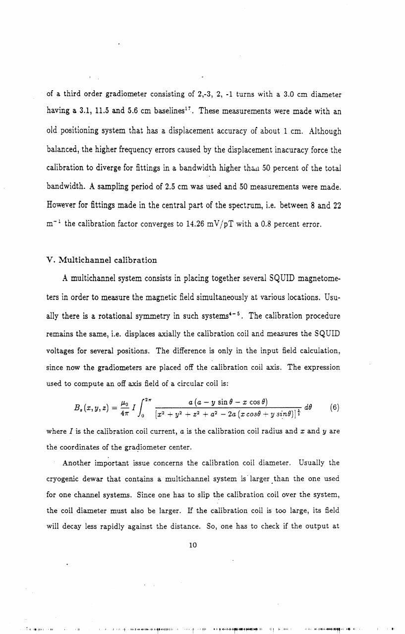
oí a third order gradiometer consisting oí 2,-3, 2, -1 turns with a 3.0 em diameter

having a 3.1, 11.5 and 5.6 cm baselines11• These measurements were made with an

old positioning system that has a displaeement aecuraey of about 1 em. Although

balanced, the higher frequeney errors eaused by the displacement inacuraey force the

calibration to diverge for fittings in a bandwidth higher th<i.ll50 percent of the total

bandwidth. A sampling period of 2.5 cm was used and 50 measurements were made.

However for fittings made in the central part of the spectrum, Le. between 8 and 22

m-1 the calibration factor converges to 14.26 fiV/pT with a 0.8 percent error.

V. Multichannel calibration

A multichannel system consists in placing together several SQUID magnetome-

ters in order to measure the magnetic field simultaneously at various locations. Usu-

ally there is a rotational symmetry in such systems4- 5. The calibration procedure

remains the same, i.e. displaces axially the calibration coil and measures the SQUID

volt ages for several positions. The difference is only in the input field calculation,

since now the gradiometers are placed off the calibration coil axis. The expression

used to compute an offaxis field oí a circular coil is:

B ( ) _ J.Lo 11211' a (a - y sin O - x cos O) dLl% x,y,z - L U

41T' o [x2 + y2 + Z2 + a2 - 2a (xcosO + y sinO)] 1(6)

where I is the calibration coil current, a is the calibration coil radius and x and y are

the coordinates of the gra4iometer center.

Another important issue concerns the calibration coil diameter. Usual1y the

cryogenic dewar that contq.ins a multichannel system is' larger .than the one used

for one channel systems. Since one has to slip the calibration coil over the system,

the coil diameter must also be larger. If the calibration coil is toe large, its field

will decay less rapidly against the distance. So, one has to check if the output at

10

'l.

... ,

a reasonable distanee from the gradiometer is small enough, if eompared with the

maximum output. This is neeessary to avoid the aliasing effect. The faetor between

maximum and minimum values we used in the above mentioned experiments was

about 150. Imagine a four ehannel system with second order gradiometers with 4,

-8, 4 turns having a 4 em b~dine, positioned at the eorners of a 2 em square. The

dewar usually used to hold this system has typically an external diameter af 33 em.

Assuming that we will use a ealibration eoi! with a 35 em diameter, if we measure

from -60 to 53 em below and above the gradiometer first eail, we will have a rate af

about 150 between maximum and minimum outputs. In order to avoid the aliasing

effect, it is shown in Fig. 10 up to which distance below the gradiometer first coi!

one has to measure, against the calibration coi! size, for different offaxis gradiometer

positions d = y'x2 + y2.

In the case of multichannel systems used for brain research, usually the gra

diometers are tilted in order to describe approximatelly the head shape. Thus, prior

to compute the Fourier transform, the input field given by Eq. (6) should be multi

plied by the cosine of the tilting angle of each gradiometer.

VI. Conc1usion

A Fourier method to calibrate multichannel SQUID systems w~ presented. One

of the main properties of this method is that the gradiometer position inside the

cryogenic dewar does not need to be known precisely. From the experimental mea-

surements we can conclude that even being highly unbalanced or if the experiment is

performed with a non accurate calibration coi! positioning system, a good value for

the fitting bandwidth is 50 percent. This corresponds to fit the experimental transfer

function by the theoretical one between 8 and 22 m- 1. The assumption that the

field is distributed uniformely over the gradiometer's area, did not seem to affect the

11

precision of the results, since the calibration errors obtained in the simulations are in

the saroe range oí the experimental ones. The best result attained in the experiments

has a 0.3 percent accuracy, the worst, 0.8 percent. These figures entitle this method

to be used to calibrate multichannel SQUID systems .

•

12

114 .'

rI" .'

REFERENCES

1 D.S. Barth, W. Sutherling, and J. Beatty, Science, 226,855 (1984).

2 P. Costa Ribeiro, A.C. Bruno, E. Parente Ribeiro,J.S. do Carmo, E. Costa

MOnteiro and A. Fonseca Costa, Advances on Biomagnetism, edited by S.J.

Williamson (Pergamon, New York, 1990) in press.

3 R. TImoniemi, R. Har, K. Reinikainen, Electroencephalogr. Clin. Neurophysiol.

58, 467 (1984).

4 J. Knuutila, S. Ahlfors, A. Ahonen, J. Hallstron, M. Kajola, O.V. Lounasmaa,

V. Vilkman, and G. Tesehe, Rev. Sei. Instrum. 58, 2145 (1987).

5 H.E. Hoenig, G. Daalmans, W. Folberth, H. Reiehenberger, S. Sehneider, and H.

Seifert, Cryogenies 29, 809 (1989).

6 P. Costa Ribeiro, S.J. Williamson, and L. Kaufman, IEEE Trans. Biomed. Eng.

Bl\1E-35, 551 (1988).

7 J.E. Zimmerman and N.V. Frederick, Appl. Phys. Lett. 18, 16 (1971).

8 G.L. Romani, S.J. Williamson, and L. Kaufman, Rev. Sei. Instrum. 53, 1815

(1982).

9 F. W. Grover, Inductance Calculations, Dover, New York (196~).

10 D.S. Buchanan· and D.N. Paulson, Advances on Biomagnetism, ~dited by S.J.

Williamson (Pergamon, New York, 1990) in press.

11 A.C. Bruno, P. Costa Ribeiro, J.P. Weid, and O.G. Symko, J. Appl. Phys. 59,

2584 (1986).

12 A.C. Bruno and P. Costa Ribeiro, J. Appl. Phys. 63,2820 (1988).

13

SERViÇO OE BIBLIOTECA E iNFORMAÇÁO - IFaSeflSICA-

13 M. Schwartz and L. Shaw, Signal Processing, (McGraw-Hill, Tokyo, 1975).

14 P. Costa Ribeiro, A.C. Bruno, C.C. Paulsen, and O.C. Symko, Rev. Sei. Instrum.

58, 1510 (1987).

15 A. Antoniou, Digital Filters Analysis and Design, (MeGraw-Hill, New York,

1979).

16 Biomagnetic Technologies, Ine. 4174 Sorrento Valley Blvd., San Diego, CA 92121.

17 A.C. Bruno and P. Costa Ribeiro, Cryogenics 23, 346 (1983).

14

.'

,.':

1.

'-t.

, >

,

Figure captions

Fig. 1 - Theoretical (squares) and experimental (continuous line) transfer func

tion amplitudes of a balanced~ second order gradiometer consisting of 4,-8, 4 turns

with a 1.5 cm diameter having a 4 cm baseline. The calibration factor was obtained

by using the proeed ure based on the mu tual ind uetanee it is 24 PT j m V.

Fig. 2 - Theoretieal (squares) and experimental (eontinuous line) transfer fune

tion amplitudes of a unbalaneed seeond order gradiometer eonsisting of 1,-2, l·turns

with a 1.5 em diameter having a 5 em baseline. The ealibration factor was obtained

by using the procedure based on the mutual induetance and it is 64 pTjmV.

Fig. 3 -' Output volt ages of theSQUID electronics of a second order gradiometer

for various positions of the ealibration coi!. The current in the calibration coi! is 8

mA.

Fig. 4 - Fourier transforms of the SQUID output for various sampling periods À

of the ealibration coi!. The gradiometer used is the same of Fig. 1.

Fig. 5 - Calibration simulation for different accuracies of the ealibration coil

. sampling period À. Curve with squares corresponds to 25 measuring positions and À

= 5 em ± 1 em. Curve with circles corresponds to 50 measuring positions and À =

2.5 cm ± 1 cm. Curve with triangles corresponds to 25 measur~ng positions and À

= 5 cm ± 1 mm. Curve with diamonds corresponds to 25 measuring positions and

À = 5 em ± 0.5 mm. The continuous line corresponds to a sampling period with no

errors.

15

Fig. 6 - Calibration curves of a balaneed seeond order gradiorneter eonsisting of

4, -8, 4 turns, with 1.5 em diarneter having a 4 em ba.seline. The da.shed line wa.s

obtained by using the input Fourier transform limits between -48 to 62 em, taking

the position of the first eoil as the origino The eontinuous line was obtained by using

the input Fourier transform limits between -5GOto 500 em.

Fig. 7 - Calibration eurve of a unbalaneed second order gradiometer eonsisting

of 1,-2, 1 turns with a 1.5 em diameter having a 5 em ba.seline. The dashed lines

eorresponds to upper and lower limits respeetively 64.65 mVjpT and 64.85 mVjpT.

Fig. 8 - Calibration curve of a balanced seeond order gradiometer eonsisting of

1, -2, 1 turns, with 3.0 em diameter having a 5 em ba.seline.

Fig. 9 - Calibration eurve of a balaneed third order gradiometer eonsisting of 2,-3,

2,-1 turns with a 3.0 em diameter having baselines 3.1, 11.5, 5.4 em. The dashed lines

eorresponds to upper and lower limits respectively 14.32 mVjpT and 14.20 mV jpT.

Fig. 10 - Distanee limits from the gradiometer first coi! against the calibration coil

diameter, that must be observed in order to avoid the aliasing effect when computing

the Fourier t:ansform of the output of a seeond order gradiometer having a 4 em

baseline. d = Vx2 + y2 corresponds to different offaxis positions.

16

114t,

c ;o• --i

. ,

~(' \

lLv ,-1

F

HF

.-.:'

F

~ r, [r--i

~

0.1

Q)4--llfJ.

~cD0.01~í .~

IT

O

5 10 15 20

Spatial FrequenC)7

•

6 G ~....•

,

-...,:::l

-;I

1l

iII

......•

:::l

-j-;~~

!ll

25 30

( . -1\I rn I, I '

.. J

FIG. 1

~1 ~O

L• r--1

f-,I.- r

~•.. " ~v ("'!

t.:......, ~-J

~

0.1 ~~

Q)~ íf1 0.01~

t

eU~~ 0.001 b

O

ri [J ~,,

...,

,

5 10 15 20 25 30

Spatial Frequency (rn-1)

FIG. 2

"

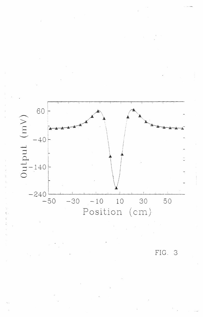
60 ~~> -

lã=.,.-., ;

:- I

'-" !

~ -40~I

, !

~ I

::) r-

. I

~ I

~ -140 L, \

~

O

\I\

iII\

\\

\1

\\

~

III

1

IrI!

-30 -10 10P .! .l 'OSltlOllr. .

-240 I I I

-' 50 30

/ ~"1~,"", \. I ,! I}\.Li J.}

50

FIG. 3

40 50

( -1rn)

o 10 20 30

Spatial Fr,equency

o

30

~

~ - - ~ lO em

>

! ,,\u __ u P - 0.0 em

/ \ -)-~ ?O

\ - _.0 em

;=- ......•

/ /

\

/ \ \ /~

'-"\ '

/ '

....•

/ \ / I

I

~

•..r ! \ ~ '

~

:~ 10 / \ /'

'/ \ " /Y \ ~/

\

/

/

FIG. 4

il4 li! 1 "1'1 •

1.04I

I I II I .

I

I

I

I, i

i1.03

I

/~

;-r-

~ ~

,~

~

i

!--.,; ,--,

O 1.02~

:.....i

~~

I

I

~

I

II

(ij 1.01I

L.

~

f----:.-v 1\

~ 1.00

' J

.1\

.~,---I

i

cU°.99!~ 1\

1-

~~

U

~

0.98

0.97 20 3040 50 60· 70, 80

Fi t ting BvV (>b)

FIG.' 5.,

,..".•....,

...

,,.

27.45 f '"'III III III

I~

I

""•....~í

I•....

> 27.35 r

\

- - t~;\ -I\

--<

F i~,

~

~ 27.25 ~\ /,

,-'-~

\/I

\ -:

~27,15,

\ /I

....;I~

1\ /l

U 27.05 t....,

\-:

/,

J\ /I

26', 95 ~l

~

-i

/~

I'-...... -- -1

-'26 85 I I I I I I I I I I I ' I I !

i

. 20 30 40 50 60 70 ·80 901 O(

Fi t ti11g

B\~T/ ~ \

I\, \'Yç. ), /

FIG, 6

~ . ,,11 ·I',~ ~if' _1411 t'IoI.~liIIllltltJ, I!~ fi"111'illl~HIIli·' ;! '1' ,. ,~,~ 111 . ~ ~I 1':lf1j,. ~JH'I~lrdl.~'''''~I•• Itl"', 11·1 III 1-',- 1"111 I II <li~ 1-' ,tl~III''''''1''1' ;11 ~.; -li!

"

69.75 ~,....I-

64.75

, -

////~ - - - - - - - - - - - - - --

30 40-..l

50 60 70

\.

,

FI"1- l.L 1" n- .. r<.-i ! iL i ~ I : }Ji I, ..• b

FIG. 7

SERViÇO DE BIBLIOTECA E INFORMAÇAO - IFaseflSICA

I?3.08 i-~ I

>23 06 [ri '. IH I

'- r. I

~2304 r

82302 tU

23.00

22.9820

~\

\\

\

\

\\.\ \

40 50

Fi t ting60 70

BT~.T ;' \'li . ,'j/ \,

\ v \/0 )

FIG. 8

80

li

14.50 ~-~!

F· I ~ •. rYi lttlnts

I

tIII

13.30 t \ ·L \ -

13002~ 30' 40 510' 60 70 80 i 9C

B1!\TlV 1;I

'-

;: 1420! -u u - - - --- - - -- -- m ---

:-' 1--- ''-~ i

~ 13.90 ~IIrL

\

FIG. 9·

. '-

"--

•

3028 38 43

ai1:·: d Ill!' !p t ie. 1.-0, , .,----,'L' JL

FIG. 10

GRADIÔMETROS SUPERCONDUTORES ACOPLADOS A SQUIDs E … · 1.1 - Biomagnetismo • o conceito de que...

Documents

Transcript of GRADIÔMETROS SUPERCONDUTORES ACOPLADOS A SQUIDs E … · 1.1 - Biomagnetismo • o conceito de que...