Exploring the Solar System using ... - repositorio.ul.pt£… · Dissertação orientada por:...
84
2017 UNIVERSIDADE DE LISBOA FACULDADE DE CIÊNCIAS DEPARTAMENTO DE FÍSICA Exploring the Solar System using stellar occultations and Gaia's sky survey João Francisco Garcia Ferreira Mestrado em Física Especialização em Astrofísica e Cosmologia Dissertação orientada por: Professor Doutor Pedro Machado (IA-FCUL)
Transcript of Exploring the Solar System using ... - repositorio.ul.pt£… · Dissertação orientada por:...
2017
UNIVERSIDADE DE LISBOA
FACULDADE DE CIÊNCIAS
DEPARTAMENTO DE FÍSICA
Exploring the Solar System using stellar occultations and
Gaia's sky survey
João Francisco Garcia Ferreira
Mestrado em Física
Especialização em Astrofísica e Cosmologia
Dissertação orientada por:
Professor Doutor Pedro Machado (IA-FCUL)

Acknowledgments
Exploring the Solar System using stellar occultations and Gaia's sky survey, João Ferreira, nº 43363
Acknowledgments
Exploring the Solar System using stellar occultations and Gaia's sky survey, João Ferreira, nº 43363
Acknowledgments
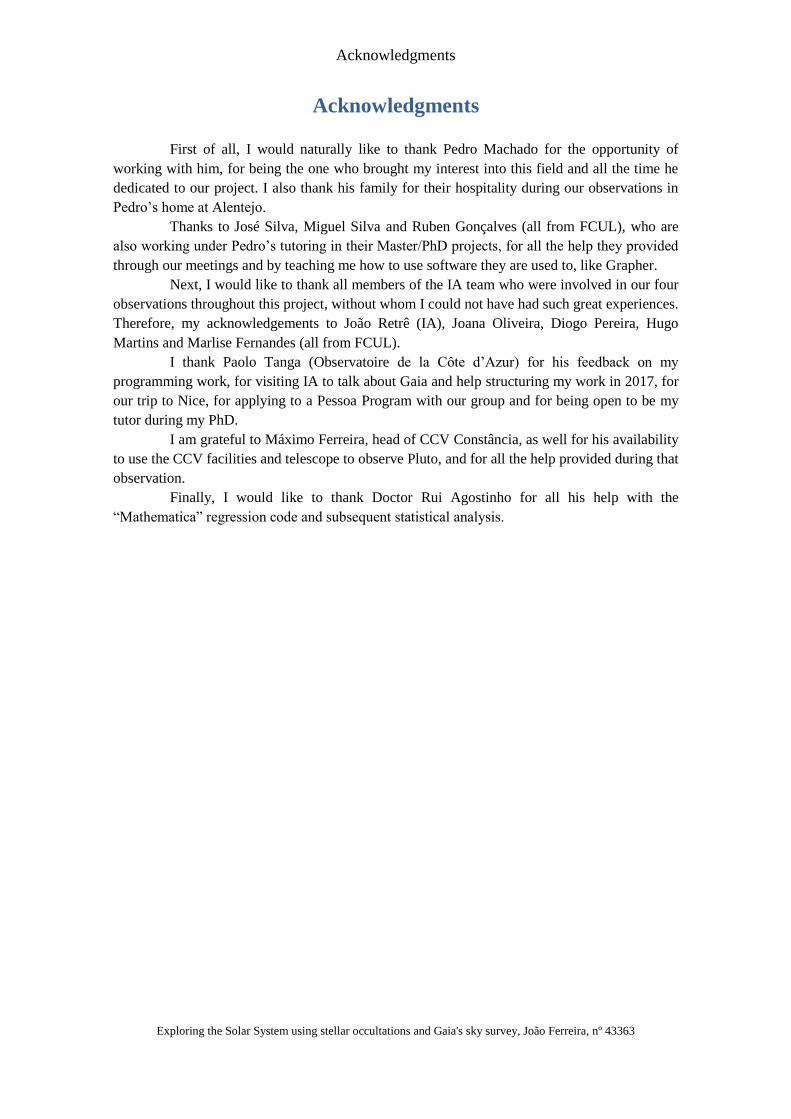
First of all, I would naturally like to thank Pedro Machado for the opportunity of
working with him, for being the one who brought my interest into this field and all the time he
dedicated to our project. I also thank his family for their hospitality during our observations in
Pedro’s home at Alentejo.
Thanks to José Silva, Miguel Silva and Ruben Gonçalves (all from FCUL), who are
also working under Pedro’s tutoring in their Master/PhD projects, for all the help they provided
through our meetings and by teaching me how to use software they are used to, like Grapher.
Next, I would like to thank all members of the IA team who were involved in our four
observations throughout this project, without whom I could not have had such great experiences.
Therefore, my acknowledgements to João Retrê (IA), Joana Oliveira, Diogo Pereira, Hugo
Martins and Marlise Fernandes (all from FCUL).
I thank Paolo Tanga (Observatoire de la Côte d’Azur) for his feedback on my
programming work, for visiting IA to talk about Gaia and help structuring my work in 2017, for
our trip to Nice, for applying to a Pessoa Program with our group and for being open to be my
tutor during my PhD.
I am grateful to Máximo Ferreira, head of CCV Constância, as well for his availability
to use the CCV facilities and telescope to observe Pluto, and for all the help provided during that
observation.
Finally, I would like to thank Doctor Rui Agostinho for all his help with the
“Mathematica” regression code and subsequent statistical analysis.

Acknowledgments
III Exploring the Solar System using stellar occultations and Gaia's sky survey, João Ferreira, nº 43363
Abstract
IV Exploring the Solar System using stellar occultations and Gaia's sky survey, João Ferreira, nº 43363
Abstract
Under the tutoring of Doctor Pedro Machado, I worked on the subject of stellar
occultations for my Seminars and Traineeship courses and this thesis as well, focusing on the
creation of independent codes that simulate and analyze this type of event. Along with the IA
team, who are referred in the “Acknowledgements” chapter, we managed to plan and execute four
observations since working together. The videos recorded during the observations were later
analyzed with a software named Tangra to obtain text files and plots of the occultation.
The simulations code was written to be user friendly, with the necessary input mostly
found in a prediction’s file. The output is two data files, one for text and one for Mathematica, to
plot the simulation and determine whether an observation is viable or not. The regression code
uses a HeavisidePi function, useful for stellar occultations, as it is the branch separation of two
constant functions. It determines the initial apparent flux, the flux drop and the beginning and
duration of the stellar occultation. A further statistical analysis is ready, which also estimates the
signal’s noise.
Besides this experimental component, the Gaia Space Mission was also analyzed,
including the first Data Release (September 2016), to determine how this type of observation can
improve due to it.
Thanks to Pedro, it’s simpler to look for stellar occultation events, and access was
granted to a global network focused on these events, allowing the group to become aware of all
the astrophysicists worldwide who dedicate their work to this as well as share results to better
understand their meaning.
A few meetings were held, including a trip to France, with one of the top astronomers
in this field, Doctor Paolo Tanga, who gave a lecture on Gaia’s influence today and helped
structuring this work for the second half of its duration.
Key words: Solar System, stellar occultations, programming, regression, small
telescopes.

Abstract
V Exploring the Solar System using stellar occultations and Gaia's sky survey, João Ferreira, nº 43363
Resumo em Português
VI Exploring the Solar System using stellar occultations and Gaia's sky survey, João Ferreira, nº 43363
Resumo em Português
Ocultações Estelares
Uma ocultação estelar ocorre quando um objecto cruza a trajectória da luz de uma
estrela do ponto de vista do observador. Este tipo de eventos não é muito frequente (alguns casos
por dia), e precisa da ajuda de aparelhos para ser detectado. Ao observar, vemos o fluxo aparente
da estrela cair num ápice, às vezes quase por completo, voltando ao normal passados alguns
segundos ou minutos. Este trabalho foca-se nas ocultações causadas por asteróides e por OTN.
As ocultações estelares, à parte das causadas pela Lua, têm sido estudadas desde os anos
50, e o aumento gradual do número de astrónomos a observar este tipo de evento tem feito com
que o número de ocultações analisadas seja cada vez maior. Hoje, por exemplo, são observadas
quase dez vezes mais ocultações do que há 20 anos atrás.
As ocultações permitem estudar pormenores do objecto que oculta, como o tamanho, o
formato, o albedo, a composição externa e, no caso de existirem, sistema de anéis e atmosfera.
Alguns casos de objectos cujo conhecimento actual depende em larga parte das ocultações são os
TNO Plutão, Eris, Makemake, Caronte e o asteróide Chariklo.
Existe uma instituição chamada IOTA que fornece previsões para várias ocultações que
permitem à equipa do IA estudar a viabilidade de uma observação. Estas previsões incluem dados
essenciais como a magnitude aparente da estrela observada, a queda prevista, a distância angular
ao Sol e à Lua e ainda a zona da superfície terrestre onde a ocultação deverá ser visível.
Códigos
Para o trabalho desta tese desenvolvi dois códigos diferentes: um para simular
ocultações e outro para as analisar.
O código de simulações foi criado após a leitura de vários dos artigos mais recentes
sobre ocultações estelares (2014-2017). Ao início foram colocadas todas as variáveis essenciais
para simular da maneira mais realista possível uma ocultação verdadeira. Foram deixados de fora
atmosferas e sistemas de anéis. Este trabalho foi desenvolvido em C++. As variáveis eram todas
arbitrárias, ou seja, o utilizador escolhia o tipo de ocultação que queria.
Após algumas alterações, o código actual conta com a seguinte escolha de parâmetros:
• Tempo de exposição da câmara;
• Diâmetro do telescópio;
• Magnitude da estrela ocultada;
• Altura da estrela ocultada no momento da ocultação;
• Duração da simulação;
• Duração e início da ocultação;
• Banda espectral usada (luz visível como base);
• Tempo UT do início da simulação.
Resumo em Português
VII Exploring the Solar System using stellar occultations and Gaia's sky survey, João Ferreira, nº 43363
O ruído da observação tem uma distribuição de Poisson. Logo, enquanto que o fluxo da
estrela é determinado a partir dos dados indicados, o desvio-padrão do ruído é a raiz quadrada
desse valor.
Quanto ao código de análise, é feita uma regressão a uma função específica conhecida
como HeavisidePi, que se trata da separação por ramos de duas funções constantes, ou seja, há
uma mudança instantânea no fluxo recebido. Esta regressão permite calcular quando começou a
ocultação, quanto tempo ela durou e quanto era o fluxo da estrela durante e fora da ocultação.
Este código foi feito em Mathematica e está a ser escrito agora em Python.
A regressão foi testada na quarta observação feita pela equipa, a única em que a
observação foi inequivocamente positiva aos olhos do código, e a duração estimada, bem como o
início, coincidiu com os valores calculados por software construído especificamente para este tipo
de observações chamado “Occult 4”.
Para a redução de dados de ficheiros de vídeo, foi utilizado um programa chamado
“Tangra”, que lê o ficheiro de vídeo e permite ao utilizador escolher a estrela ocultada bem como
até três estrelas-guia. Depois, é feito um gráfico com os dados, a partir do qual podemos aceder à
tabela que é usada no “Occult 4” e no código de regressão.
Observações
Graças à equipa do IA, foram feitas quatro observações desde o início do trabalho desta
tese a quatro objectos diferentes: Psyche, Plutão, Ambrosia e Daphne.
A observação de Psyche, a 26 de Abril de 2016, no Alentejo foi gorada devido ao mau
tempo, pois durante a noite do evento, ainda conseguimos ver o campo de observação, sendo
visível até o próprio asteróide. Não conseguimos recolher dados deste evento.
A ocultação de Plutão, a 16 de Julho, em Constância estava incorporada num conjunto
de observações que tinha como objectivo uma ocultação três dias depois. A nossa equipa
participou a pedido do investigador Bruno Sicardy (Observatoire de Paris). Contámos com a
colaboração do director do CCV Constância, Máximo Ferreira, e a ocultação foi dias depois
confirmada como positiva pelo próprio Bruno Sicardy, estando a queda quase ao nível do ruído.
Há a hipótese não confirmada de termos visto um sinal (“flash central”) causado pela atmosfera
de Plutão.
A 22 de Agosto, foi a vez de observar Ambrosia no Alentejo. Esta ocultação decorreu
sem problemas, e conseguimos observar o campo da ocultação, mas não foi visualizada nenhuma
ocultação. A queda prevista do fluxo aparente era grande (quase 99%), mas nada do género foi
observado. Isto pode ter acontecido por a trajectória do asteróide estar errada nas previsões, o que
fez com que o nosso ponto de observação não estivesse dentro da zona de observação da
ocultação, ao contrário do que estava previsto.
A última ocultação feita pela equipa do IA foi a 2 de Março de 2017 a Daphne, também
no Alentejo. Apesar do tempo instável, conseguimos observar o evento e tivemos uma ocultação
inequívoca. O resultado mais surpreendente foi o facto de a ocultação ter sido bastante mais longa
que a duração máxima prevista (19,4 segundos em vez de 16,8) o que sugere que o asteróide
observado é na verdade maior do que se pensava e que terá um formato oblongo. A queda de
fluxo aparente foi ligeiramente maior que o previsto (63% em vez de 60%), mas esta diferença
está ao nível do ruído pelo que pode não ter um significado físico. Esta análise de dados foi feita
com o código de regressão e também com o “Occult 4”.
Resumo em Português
VIII Exploring the Solar System using stellar occultations and Gaia's sky survey, João Ferreira, nº 43363
Gaia
A missão espacial Gaia é um projecto da ESA, tendo o telescópio sido lançado em 2013.
A primeira divulgação de dados ocorreu em Setembro de 2016, e alguns desses resultados já estão
a ser usados nas previsões de ocultações estelares. Estão previstas três datas para divulgação de
dados até 2022.
O Gaia sucedeu ao Hipparcos na missão de medir a posição das estrelas. A incerteza na
posição vai diminuir de 1 milissegundo de arco para 10 microssegundos de arco, um factor de
100. Essa diminuição na incerteza permitirá um aumento na confiança nas previsões de ocultações
estelares, através da diminuição da incerteza da trajectória do caminho de sombra do asteróide na
superfície terrestre. Isto não só permitirá prever mais ocultações, como deverá diminuir a
quantidade de observações negativas.
Um exemplo particular do uso do Gaia foi na ocultação de Plutão de 19 de Julho, onde
os dados do Gaia sobre a estrela ocultada foram disponibilizados com antecedência, alterando a
zona de sombra através de uma translacção desta para Sul na superfície terrestre em mais de 700
km!
Resultados, Conclusões e Trabalho Futuro
Apesar de recentes, as ocultações são já uma componente fundamental no estudo da
história do Sistema Solar, em particular de corpos pequenos. As 4 observações em que tive
oportunidade de participar permitiram-me ganhar experiência e perceber quais as principais
limitações de uma observação nesta área. Dado o panorama global, 2 observações positivas em 3
realizadas (sem contar com Psyche, por causa de mau tempo) é um excelente resultado que
comprova a robustez do planeamento feito pela equipa do IA.
Um resultado interessante foi a análise de Daphne, que parece ser bastante maior do que
anteriormente se pensava (cerca de 15% maior). Já a observação a Plutão foi parte de uma
experiência maior, e há uma hipótese de termos visto a sua atmosfera.
O código que simula ocultações é neste momento bastante realista, podendo ser usado
a partir de uma previsão típica, e permitindo o teste de situações-limite na regressão. Já a regressão
está operacional para ocultações longas e/ou claras. Nestes regimes, determina a um bom grau os
parâmetros físicos mais importantes, e para o caso de Daphne os resultados foram confirmados
com os obtidos a partir do Occult4, uma ferramenta criada especificamente com este fim.
Já o Gaia começa a ser usado nas previsões do IOTA, diminuindo significativamente as
incertezas associadas. Isto vai não só permitir mais resultados positivos, mas também motivar os
astrónomos a ver casos mais complicados, com quedas fracas ou durações curtas.
No seguimento desta tese, irei fazer o doutoramento na Universidade de Nice, com o
Doutor Paolo Tanga como orientador e o Doutor Pedro Machado como co-orientador, também
sob o tema de ocultações estelares. Não só vamos aprofundar o trabalho realizado no âmbito desta
tese, mas também partir para projectos mais ambiciosos, possíveis com a segunda divulgação de
dados do Gaia, prevista para Abril de 2018 que, entre outros resultados, irá incluir astrometria de
asteróides.
Resumo em Português
IX Exploring the Solar System using stellar occultations and Gaia's sky survey, João Ferreira, nº 43363
Palavras-chave: Sistema Solar, ocultações estelares, programação, regressão,
pequenos telescópios.
Table of Contents
X Exploring the Solar System using stellar occultations and Gaia's sky survey, João Ferreira, nº 43363
Table of Contents
Acknowledgments ............................................................................................................ II
Abstract ........................................................................................................................... IV
Resumo em Português .................................................................................................... VI
Ocultações Estelares ................................................................................................... VI
Códigos ....................................................................................................................... VI
Observações ............................................................................................................... VII
Gaia ........................................................................................................................... VIII
Resultados, Conclusões e Trabalho Futuro .............................................................. VIII
Table of Contents ............................................................................................................. X
List of Images ................................................................................................................ XII
List of Graphics ........................................................................................................... XVI
List of Tables ............................................................................................................. XVIII
Chapter 1: Thesis Overview ............................................................................................. 1
1.1: Motivations ........................................................................................................ 1
1.2: Objectives .......................................................................................................... 2
1.3: Scientific Context .............................................................................................. 2
1.4: Thesis Structure ................................................................................................. 3
Chapter 2: Introduction ..................................................................................................... 5
Chapter 3: Simulations ................................................................................................... 11
Chapter 4: Regression ..................................................................................................... 15
Chapter 5: Tangra – Data Reduction Software ............................................................... 23
Chapter 6: Observations ................................................................................................. 27
6.1: Psyche .............................................................................................................. 27

Table of Contents
XI Exploring the Solar System using stellar occultations and Gaia's sky survey, João Ferreira, nº 43363
6.2: Pluto ................................................................................................................. 30
6.3: Ambrosia ......................................................................................................... 32
6.4: Daphne ............................................................................................................. 34
Chapter 7: PlanOccult Results ........................................................................................ 37
Chapter 8: Gaia’s contributions ...................................................................................... 43
Chapter 9: Transits and Exoplanets – Connections with Occultations ........................... 49
Chapter 10: Conclusions ................................................................................................. 53
Chapter 11: Future Work ................................................................................................ 55
Bibliography ................................................................................................................... 59
Appendix ........................................................................................................................ 63
List of Images
XII Exploring the Solar System using stellar occultations and Gaia's sky survey, João Ferreira, nº 43363
List of Images
Image 2.1 - Example of the light of a star changing with time because of an occulting
object with an atmosphere and rings. Image courtesy of Bruno Sicardy. ..................... 6
Image 2.2 – Example of an occultation prediction. It includes the object’s path and
physical properties of both objects and the event. The region between the thick lines is
the asteroid’s shadow path, while the regions between a dotted line and a thick line
represent 1σ uncertainty. ........................................................................................ 7
Image 2.3 – Gaia spacecraft. (Source: Gaia’s homepage, http://sci.esa.int/gaia/) ........ 10
Image 3.1 – Parameter input before running the code. ............................................. 13
Image 3.2 – Marsaglia Polar Method. X1 and X2 are random numbers following a
Normal distribution N(0,1). .................................................................................. 13
Image 3.3 – Extra calculations: how big is the object, given the simulation. .............. 14
Image 3.4 – Example of data output to text and Mathematica files. For the Mathematica
plot, the minimum and maximum. Are also recalculated. ........................................ 14
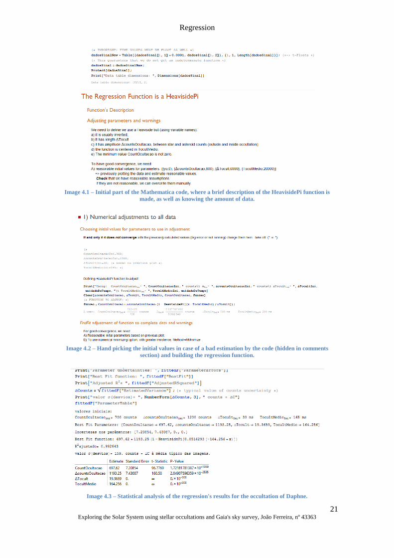
Image 4.1 – Initial part of the Mathematica code, where a brief description of the
HeavisidePi function is made, as well as knowing the amount of data. ...................... 21
Image 4.2 – Hand picking the initial values in case of a bad estimation by the code
(hidden in comments section) and building the regression function. ......................... 21
Image 4.3 – Statistical analysis of the regression's results for the occultation of Daphne.
......................................................................................................................... 21
Image 5.1 – Initial menu of Tangra. ...................................................................... 23
Image 5.2 – Opening menu of AOTA. ................................................................... 25
Image 6.1 – Example of Starry Night File: Triton is the target, the other objects are
alignment stars and the angular distance to the Moon is verified. ............................. 28
Image 6.2 - Example of IOTA's star maps: a 30' rectangle. The bigger the dot, the
brighter the star is. .............................................................................................. 28
Image 6.3 – Psyche predictions by IOTA. .............................................................. 29
Image 6.4 – Telescope used for this observation, Ambrosia and Daphne, along with the
team. From left to right: Joana Oliveira, Marlise Fernandes, Diogo Pereira, João Retrê
and me (Pedro was also part of the team). .............................................................. 30
List of Images
XIII Exploring the Solar System using stellar occultations and Gaia's sky survey, João Ferreira, nº 43363
Image 6.5 – Pluto predictions by Bruno Sicardy. .................................................... 31
Image 6.6 – Occulting team (minus Pedro) and telescope used. On the left, Máximo
Ferreira. ............................................................................................................. 31
Image 6.7 – Ambrosia predictions by IOTA. .......................................................... 33
Image 6.8 - Daphne predictions by IOTA. ............................................................. 34
Image 6.9 – Pedro and I after the whole team had already set up the telescope. .......... 36
Image 7.1 - Path correction for asteroid GZ32, as calculated by Lecacheux Jean
(Observatoire du Pic du Midi) thanks to four positive (green) and eleven negative (red)
observations. ...................................................................................................... 40
Image 7.2 – Haumea prediction by IOTA. ............................................................. 40
Image 7.3 – Uranus’s rings observed through a small telescope. .............................. 41
Image 7.4 - Live stream of the NEO 2014 JO25. The second brightest spot on the mid-
center section of the left image moves in the span of a few seconds to a different
position on the field. Video courtesy of Gerhard Dangl (IAU Minor Planet Center
observatory, Nonndorf). ....................................................................................... 42
Image 8.1 – Schematics of the 5 Lagrangian Points in the Sun-Earth system. Future
space telescope James Webb is represented in L2, where Gaia is presently located. L3,
L4 and L5 match Earth's orbit, while L1 has Earth and the Sun facing opposite
directions. L2 has Earth and the Sun in the same direction. Source:
https://www.nasa.gov/topics/universe/features/webb-l2.html. .................................. 43
Image 8.2 – Comparison between actual positions and predictions for the Daphne
occultation. The second brightest object in the first image is Daphne, which is not
shown in the Starry Night picture. ......................................................................... 44
Image 8.3 – Improvement of the uncertainty region throughout 2013 (1st image), 2015
(2nd) and 2017 (3rd). All images by IOTA-ES. ........................................................ 45
Image 8.4 – Correction to the shadow path made with Gaia data. European teams
represented by green lines. Images courtesy of Paolo Tanga. The shadow seems to go at
least 1 000 km south. ........................................................................................... 46
Image 9.1 – Venus transit. This event lasted about 6 hours. Image courtesy of Pedro
Machado. ........................................................................................................... 49
Image 9.2 – Mercury transit as observed at FCUL. The arrow points at the planet. We
used an H-alpha band. ......................................................................................... 50
List of Images
XIV Exploring the Solar System using stellar occultations and Gaia's sky survey, João Ferreira, nº 43363
Image 11.1 - Schematics Paolo made for my PhD. I will be focusing on the tasks at the
right, namely data reduction and exploring interesting and/or limit cases for stellar
occultations. ....................................................................................................... 56
Image 11.2 - Triton's shadow path and predictions, with information from Gaia’s DR2
for the star’s astrometry. Image by Bruno Sicardy. ................................................. 57
Image 11.3 - Pedro, myself and Paolo at the C2PU 1-meter telescope. ...................... 57

List of Images
XV Exploring the Solar System using stellar occultations and Gaia's sky survey, João Ferreira, nº 43363
List of Graphics
XVI Exploring the Solar System using stellar occultations and Gaia's sky survey, João Ferreira, nº 43363
List of Graphics
Graphic 2.1 – Amount of positive events by year from 1997 to 2006. For 2016/17,
PlanOccult results were used to estimate the amount of positive events. Image by
Frappa et al (2011). ............................................................................................... 5
Graphic 2.2 – Total amount of observations (negative + positive) by telescope aperture
from 1997 to 2006. Image by Frappa et al (2011). .................................................... 7
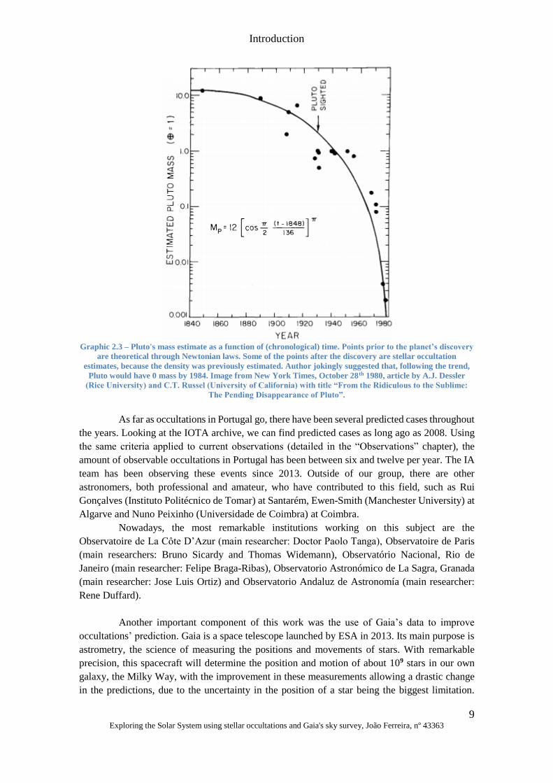
Graphic 2.3 – Pluto's mass estimate as a function of (chronological) time. Points prior to
the planet’s discovery are theoretical through Newtonian laws. Some of the points after
the discovery are stellar occultation estimates, because the density was previously
estimated. Author jokingly suggested that, following the trend, Pluto would have 0 mass
by 1984. Image from New York Times, October 28th 1980, article by A.J. Dessler (Rice
University) and C.T. Russel (University of California) with title “From the Ridiculous
to the Sublime: The Pending Disappearance of Pluto”. .............................................. 9
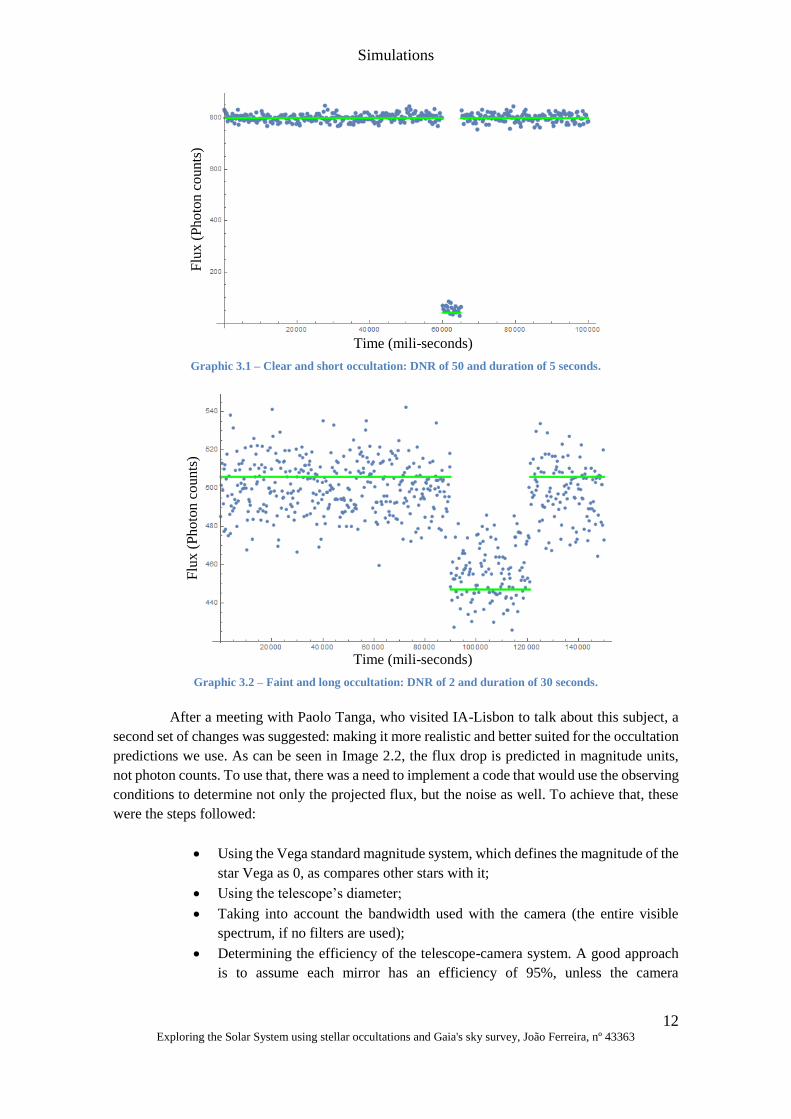
Graphic 3.1 – Clear and short occultation: DNR of 50 and duration of 5 seconds. ...... 12
Graphic 3.2 – Faint and long occultation: DNR of 2 and duration of 30 seconds. ....... 12
Graphic 4.1 – Result of the regression test for an occultation of 2.5 seconds with DNR =
20. ..................................................................................................................... 16
Graphic 4.2 – Result of the regression test for an occultation of 35 seconds, with DNR =
2........................................................................................................................ 16
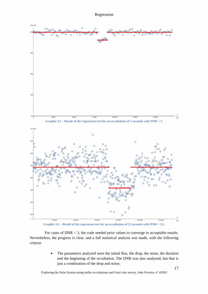
Graphic 4.3 – Result of the regression test for an occultation of 2 seconds with DNR =
5........................................................................................................................ 17
Graphic 4.4 – Result of the regression test for an occultation of 25 seconds with DNR =
2.5. .................................................................................................................... 17
Graphic 4.5 - Merit factor vs Global Error. The global error is the quadratic sum of the
duration and drop errors. ...................................................................................... 20
Graphic 5.1 – Example of the output of Tangra. A text file with Flux vs Time is also
created. This is a real occultation, but no details about it are known, as only the video
file was available. ............................................................................................... 24
Graphic 5.2 – Posterior analysis to this example, including this time the guiding star.
The two stars seem to have similar fluxes. ............................................................. 24
Graphic 5.3 – Example of a lightcurve built by AOTA. The different near-vertical
slopes are the program's initial and final estimation of where the occultation begins. .. 26
List of Graphics
XVII Exploring the Solar System using stellar occultations and Gaia's sky survey, João Ferreira, nº 43363
Graphic 6.1 – Lightcurves of the occulted star (blue) and guiding stars (others). Around
4 440s (UT), we see the occultation. The red dotted lightcurve rises by the end due to
the star being behind the timestamp of the camera, which tampered with the
measurements. .................................................................................................... 32
Graphic 6.2 – Occultation of Ambrosia, with a binning of 16 frames per point. ......... 33
Graphic 6.3 – Occultation of Daphne. ................................................................... 35
Graphic 6.4 – Daphne occultation analyzed by AOTA (zoomed in on the occultation
zone). ................................................................................................................ 35
Graphic 7.1 – Kalliope occultation observed and analyzed in Italy by Pietro Baruffetti
(Gruppo Astrofili Massesi). .................................................................................. 38
Graphic 7.2 – Aegle occultation studied with Tangra by Carlos Perelló. Blue data is
from the occulted star, and green data from a guiding star. ...................................... 38
Graphic 7.3 - Siegena occultation as seen by Juan Rovira Picañol and his team at Moià.
......................................................................................................................... 39
Graphic 7.4 - Nassovia occultation as seen by Jan Maarten Winkel and his team from
Zeddam. ............................................................................................................. 39
Graphic 7.5 – Doubtful, and most likely negative, observation by Tim Haymes (British
Astronomical Association). .................................................................................. 41
Graphic 8.1 - Size range of asteroids detectable by Gaia, by Solar System Zone. Limit
magnitude of 20 used. Image courtesy of Paolo Tanga. ........................................... 47
Graphic 8.2 - Gaia astrometry uncertainty vs Data Release. Image courtesy of Paolo
Tanga. ............................................................................................................... 47
Graphic 9.1 – Exoplanets sorted by year of discovery and first method used. 2014 and
2016 are spiked because of Kepler Data Releases. Plot by NASA exoplanet archive,
whose link is at the top right corner. ...................................................................... 50
Graphic 9.2 - Similarities between observing an exoplanetary transit and an occultation.
......................................................................................................................... 51
List of Tables
XVIII Exploring the Solar System using stellar occultations and Gaia's sky survey, João Ferreira, nº 43363
List of Tables
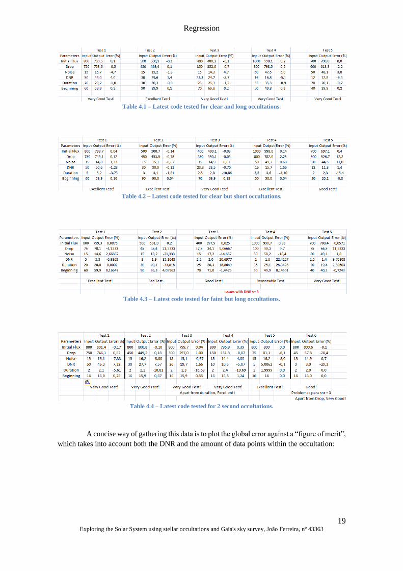
Table 4.1 – Latest code tested for clear and long occultations. ................................. 19
Table 4.2 – Latest code tested for clear but short occultations. ................................. 19
Table 4.3 – Latest code tested for faint but long occultations. .................................. 19
Table 4.4 – Latest code tested for 2 second occultations. ......................................... 19
List of Tables
XIX Exploring the Solar System using stellar occultations and Gaia's sky survey, João Ferreira, nº 43363
Thesis Overview
Exploring the Solar System using stellar occultations and Gaia's sky survey, João Ferreira, nº 43363
1
Chapter 1: Thesis Overview
1.1: Motivations
During my first year of the Physics Master at FCUL, I had a Planetary Systems Course
taught by Pedro. His captivating lessons and my interest on this subject pushed me into wanting
to work with him. Pedro was kind enough to agree on the tutoring and presented three choices:
• Working on spectroscopic analysis of planetary atmospheres;
• Developing a tool built for Venus’s atmospheres to study other planets,
mainly the gas giants;
• The study of asteroids and TNO, via stellar occultations.
With these options, it would have been natural to choose planetary atmospheres. After
all, not only is that Pedro’s field of expertise, but two of his PhD students are also working on
this subject, as well as one of my friends who is in my year of the Master’s program. To add to
that, the Bachelor’s project associated with astrophysics also revolved around planetary
atmospheres, namely studying the atmosphere of Uranus with ALMA data.
Despite all these factors, the stellar occultations ended up grabbing my attention. For
the same reason I worked with Uranus during my Bachelor, I ended up choosing this subject: I
was curious to see what it had to offer.
Even though it was a new field for me, I wasn’t completely unaware of what stellar
occultations were. I had already attended a lecture on the subject by Pedro himself, through a
programme by the IA (then CAAUL). With the help of that lecture and some material Pedro gave
me, soon this appeared to be the right choice.
Stellar occultations are an interesting field of Astronomy because it is an innovative
method for studying small bodies in the Solar System. Several observations on the same object
may allow a detailed analysis, and it usually does not require a big telescope, making it easier to
prepare an observation ahead of time. Since small telescopes are good enough for stellar
occultations, we can even make observations from our own homes, as we did three times
regarding this thesis.
Lastly, another reason I was motivated to choose stellar occultations was its similarities
with planetary transits, an increasingly important method of detecting candidate exoplanets,
another field that I am deeply interested in. If I want to work on exoplanets in the future, my
background on occultations might be of major help.
Thesis Overview
Exploring the Solar System using stellar occultations and Gaia's sky survey, João Ferreira, nº 43363
2
1.2: Objectives
There were four main goals in this work:
• Develop software that can easily simulate the conditions under which a stellar
occultation will occur when given details about the star (position in the sky and
apparent flux) and the telescope-camera system (telescope size, efficiency and
exposure time);
• Build software that, through a text file with the data of an observation or
simulation, makes a regression that determines physical parameters of the
occulting body (difference in apparent flux, occultation duration and
occultation beginning), while also calculating the noise to determine whether
the parameters are significant;
• Studying Gaia’s influence on the prediction of stellar occultations;
• Observing occultations with the IA team to put all of the theoretical work to the
test.
1.3: Scientific Context
One of the biggest mysteries of our Solar System is its origin: how was it in the
beginning? The current best answer is the Nice Model, which suggests, among other things, that
the gas giants were primarily closer than they are in the present and that planets formed through
accretion of material.
Still, there are several open questions, and the other planetary systems that are being
discovered through the study of exoplanets seem to suggest that this model has flaws. As such,
we need to study objects that can be traced back to the initial moments of the Solar System.
The best candidate objects for this kind of study are asteroids, comets and TNO. They
all have in common the fact that they are “small” objects, by which we mean smaller than planets
(and a few moons). The fact that very few of these objects have atmospheres also makes them
extremely cold, because most of the time they are further away from the Sun than Mars. As such,
they are difficult to observe.
All of these objects can be studied through stellar occultations, although few cases of
occultations by comets have been published. With this method, astronomers can estimate the
shape and density of the object (if we know its mass), study its inner and outer structure and the
possible presence of other characteristics, such as atmospheres and rings. With an international
collaboration, even with the almost exclusive use of small telescopes, this method can reach
results as good as big telescope and space mission results.
Thesis Overview
3 Exploring the Solar System using stellar occultations and Gaia's sky survey, João Ferreira, nº 43363
1.4: Thesis Structure
After this small chapter dedicated to giving the thesis context, an introduction will
follow, detailing what stellar occultations are and their use in Astronomy, focusing on the work
in the 21st century, and an overview on the Gaia Space Telescope.
Next to the introduction, there is a chapter dedicated to the programming work, namely
the simulations code developed as well as the regression code that helps determine the physical
parameters studied during an occultation. There is also a chapter dedicated to specific software
called “Tangra” used to reduce data from observations.
Following is the observations chapter, where all four observations made by the IA team
in the last year and a half are detailed. There is also a discussion on all of the available results
(one of the observations failed due to bad weather). There is also a chapter dedicated to the
worldwide results on this field, available through the PlanOccult mailing list, mentioning the most
discussed topics and the most observed events.
Afterwards, Gaia’s importance in this field is explained through details and examples
of predictions improved to the data available from the first Data Release of this mission.
After Gaia, there is a chapter dedicated to the similarities between stellar occultations
and other events such as transits and eclipses, to further put into context how this work can relate
to other areas in Astronomy, like exoplanets.
Finally, there is a chapter for the conclusions made from the work of this thesis, and
another one for the future work to be made, not only in terms of observations, but projects for a
PhD as well. A bibliography with all the sources used for this thesis is the last bit of the work’s
main body.
By the end there is an appendix, with all the abbreviations explained, a list of all the
technical terms used and their meaning and the definition of some words the reader might not be
familiar with.

Thesis Overview
4 Exploring the Solar System using stellar occultations and Gaia's sky survey, João Ferreira, nº 43363
Introduction
5 Exploring the Solar System using stellar occultations and Gaia's sky survey, João Ferreira, nº 43363
Chapter 2: Introduction
A stellar occultation is an event in which a certain object crosses the trajectory of a star’s
light from the observer’s perspective. Considering how small stars look in the sky and how
scattered they seem, even when taken into account stars the human eye usually can’t see, this is
not a frequent phenomenon, and we must be expecting it in order to see something.
When it does happen, though, we watch as the star loses some of its flux momentarily,
in some cases even seeming like the star disappears completely. This can be caused by any object
in the Solar System, and is usually observed when it is an asteroid, comet or TNO. Because of its
size, the Moon is by far responsible for the biggest amount of occultations, but will not be
considered in this work because of how different those are from the occultations due to small
objects in terms of angular size. [Santos-Sanz, P. et al. (2014)]
The first occultations observed were naturally caused by the Moon and other planets of
the Solar System, not only because of their bigger angular size, but because we know their orbits
with much greater precision than other bodies. These have been happening since the 50’s.
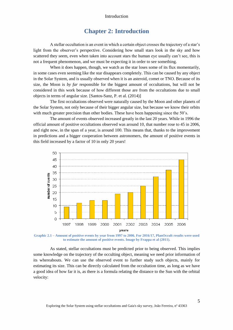
The amount of events observed increased greatly in the last 20 years. While in 1996 the
official amount of positive occultations observed was around 10, that number rose to 45 in 2006,
and right now, in the span of a year, is around 100. This means that, thanks to the improvement
in predictions and a bigger cooperation between astronomers, the amount of positive events in
this field increased by a factor of 10 in only 20 years!
Graphic 2.1 – Amount of positive events by year from 1997 to 2006. For 2016/17, PlanOccult results were used
to estimate the amount of positive events. Image by Frappa et al (2011).
As stated, stellar occultations must be predicted prior to being observed. This implies
some knowledge on the trajectory of the occulting object, meaning we need prior information of
its whereabouts. We can use the observed event to further study such objects, mainly for
estimating its size. This can be directly calculated from the occultation time, as long as we have
a good idea of how far it is, as there is a formula relating the distance to the Sun with the orbital
velocity:
Introduction
6 Exploring the Solar System using stellar occultations and Gaia's sky survey, João Ferreira, nº 43363
𝑣 ≈ √𝐺𝑀
𝑟
Where G is the Gravitational Constant (6.673*10-11 Nm2kg-2), M is the mass of the Sun
(2*1030 kg) and r is the distance to the object. Caution is still needed, because the estimated
velocity in the occultation is merely the tangential component, leaving the normal component
unknown. Despite this, it will allow a good estimate of the object’s size. This is obtained from
Kepler’s Laws when approximating for an object (Sun) much more massive than the other
(asteroid/comet/TNO).
If many observations in different points of the globe are made to the same occultation,
we may also be able to estimate other parameters, such as the object’s shape, density (in case of
a known mass), internal structure through the density and external structure through the albedo.
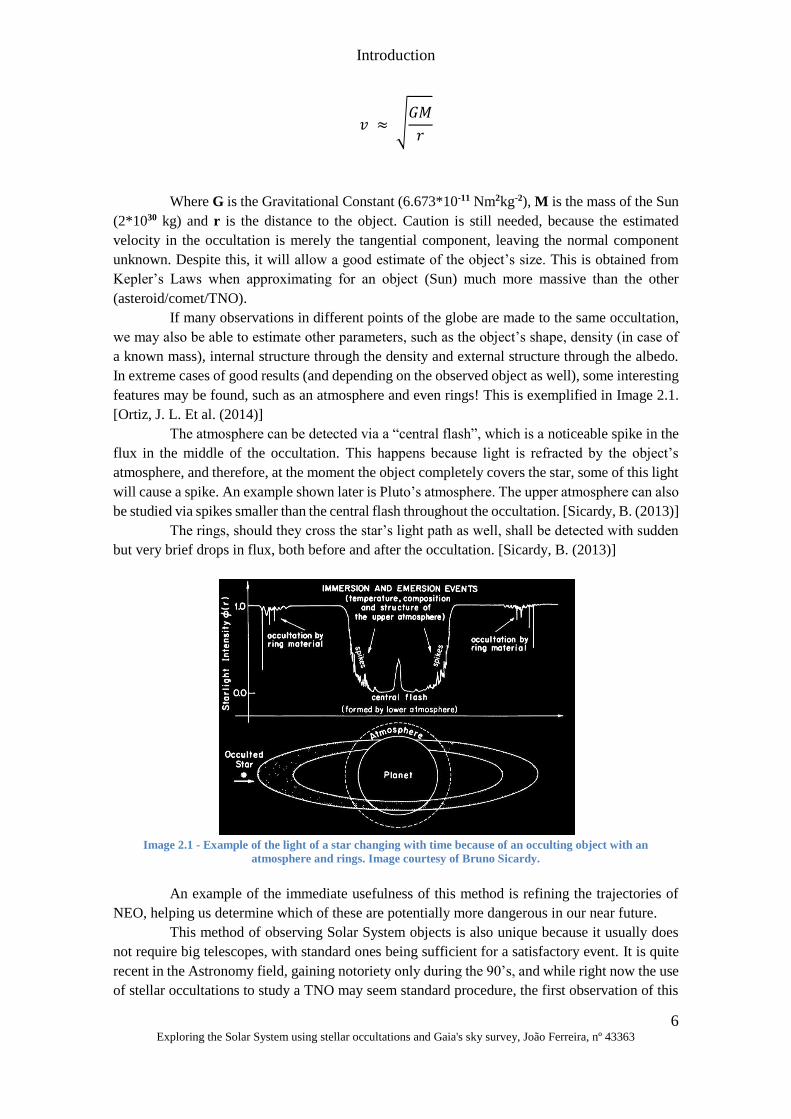
In extreme cases of good results (and depending on the observed object as well), some interesting
features may be found, such as an atmosphere and even rings! This is exemplified in Image 2.1.
[Ortiz, J. L. Et al. (2014)]
The atmosphere can be detected via a “central flash”, which is a noticeable spike in the
flux in the middle of the occultation. This happens because light is refracted by the object’s
atmosphere, and therefore, at the moment the object completely covers the star, some of this light
will cause a spike. An example shown later is Pluto’s atmosphere. The upper atmosphere can also
be studied via spikes smaller than the central flash throughout the occultation. [Sicardy, B. (2013)]
The rings, should they cross the star’s light path as well, shall be detected with sudden
but very brief drops in flux, both before and after the occultation. [Sicardy, B. (2013)]
Image 2.1 - Example of the light of a star changing with time because of an occulting object with an
atmosphere and rings. Image courtesy of Bruno Sicardy.
An example of the immediate usefulness of this method is refining the trajectories of
NEO, helping us determine which of these are potentially more dangerous in our near future.
This method of observing Solar System objects is also unique because it usually does
not require big telescopes, with standard ones being sufficient for a satisfactory event. It is quite
recent in the Astronomy field, gaining notoriety only during the 90’s, and while right now the use
of stellar occultations to study a TNO may seem standard procedure, the first observation of this
Introduction
7 Exploring the Solar System using stellar occultations and Gaia's sky survey, João Ferreira, nº 43363
kind for a TNO other than Pluto happened only in 2009! [Ortiz, J. L. Et al. (2014)] There is clearly
much to be done still.
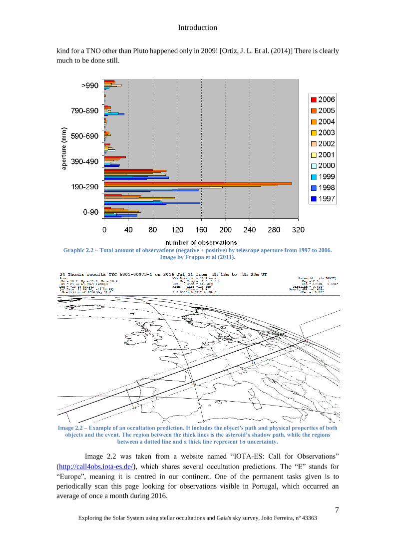
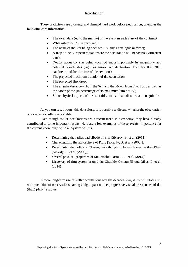
Graphic 2.2 – Total amount of observations (negative + positive) by telescope aperture from 1997 to 2006.
Image by Frappa et al (2011).
Image 2.2 – Example of an occultation prediction. It includes the object’s path and physical properties of both
objects and the event. The region between the thick lines is the asteroid’s shadow path, while the regions
between a dotted line and a thick line represent 1σ uncertainty.
Image 2.2 was taken from a website named “IOTA-ES: Call for Observations”
(http://call4obs.iota-es.de/), which shares several occultation predictions. The “E” stands for
“Europe”, meaning it is centred in our continent. One of the permanent tasks given is to
periodically scan this page looking for observations visible in Portugal, which occurred an
average of once a month during 2016.
Introduction
8 Exploring the Solar System using stellar occultations and Gaia's sky survey, João Ferreira, nº 43363
These predictions are thorough and demand hard work before publication, giving us the
following core information:
• The exact date (up to the minute) of the event in each zone of the continent;
• What asteroid/TNO is involved;
• The name of the star being occulted (usually a catalogue number);
• A map of the European region where the occultation will be visible (with error
bars);
• Details about the star being occulted, most importantly its magnitude and
celestial coordinates (right ascension and declination, both for the J2000
catalogue and for the time of observation);
• The projected maximum duration of the occultation;
• The projected flux drop;
• The angular distance to both the Sun and the Moon, from 0º to 180º, as well as
the Moon phase (in percentage of its maximum luminosity);
• Some physical aspects of the asteroids, such as size, distance and magnitude.
As you can see, through this data alone, it is possible to discuss whether the observation
of a certain occultation is viable.
Even though stellar occultations are a recent trend in astronomy, they have already
contributed to some important results. Here are a few examples of these events’ importance for
the current knowledge of Solar System objects:
• Determining the radius and albedo of Eris [Sicardy, B. et al. (2011)];
• Characterizing the atmosphere of Pluto [Sicardy, B. et al. (2003)];
• Determining the radius of Charon, once thought to be much smaller than Pluto
[Sicardy, B. et al. (2006)];
• Several physical properties of Makemake [Ortiz, J. L. et al. (2012)];
• Discovery of ring system around the Chariklo Centaur [Braga-Ribas, F. et al.
(2014)].
A more long-term use of stellar occultations was the decades-long study of Pluto’s size,
with such kind of observations having a big impact on the progressively smaller estimates of the
(then) planet’s radius.
Introduction
9 Exploring the Solar System using stellar occultations and Gaia's sky survey, João Ferreira, nº 43363
Graphic 2.3 – Pluto's mass estimate as a function of (chronological) time. Points prior to the planet’s discovery
are theoretical through Newtonian laws. Some of the points after the discovery are stellar occultation
estimates, because the density was previously estimated. Author jokingly suggested that, following the trend,
Pluto would have 0 mass by 1984. Image from New York Times, October 28th 1980, article by A.J. Dessler
(Rice University) and C.T. Russel (University of California) with title “From the Ridiculous to the Sublime:
The Pending Disappearance of Pluto”.
As far as occultations in Portugal go, there have been several predicted cases throughout
the years. Looking at the IOTA archive, we can find predicted cases as long ago as 2008. Using
the same criteria applied to current observations (detailed in the “Observations” chapter), the
amount of observable occultations in Portugal has been between six and twelve per year. The IA
team has been observing these events since 2013. Outside of our group, there are other
astronomers, both professional and amateur, who have contributed to this field, such as Rui
Gonçalves (Instituto Politécnico de Tomar) at Santarém, Ewen-Smith (Manchester University) at
Algarve and Nuno Peixinho (Universidade de Coimbra) at Coimbra.
Nowadays, the most remarkable institutions working on this subject are the
Observatoire de La Côte D’Azur (main researcher: Doctor Paolo Tanga), Observatoire de Paris
(main researchers: Bruno Sicardy and Thomas Widemann), Observatório Nacional, Rio de
Janeiro (main researcher: Felipe Braga-Ribas), Observatorio Astronómico de La Sagra, Granada
(main researcher: Jose Luis Ortiz) and Observatorio Andaluz de Astronomía (main researcher:
Rene Duffard).
Another important component of this work was the use of Gaia’s data to improve
occultations’ prediction. Gaia is a space telescope launched by ESA in 2013. Its main purpose is
astrometry, the science of measuring the positions and movements of stars. With remarkable
precision, this spacecraft will determine the position and motion of about 109 stars in our own
galaxy, the Milky Way, with the improvement in these measurements allowing a drastic change
in the predictions, due to the uncertainty in the position of a star being the biggest limitation.
Introduction
10 Exploring the Solar System using stellar occultations and Gaia's sky survey, João Ferreira, nº 43363
Thus, the observation of a much greater amount of events will become possible, especially for
fainter and/or shorter occultations.
Image 2.3 – Gaia spacecraft. (Source: Gaia’s homepage, http://sci.esa.int/gaia/)
The first Data Release became available in last year’s September [Gaia Collaboration
et al. (2016)], meaning the work on this field is just now getting started, and the near future might
see an explosion in the amount of accurate predictions! This is just the first of many Data Releases,
being the most incomplete one as well. There are plans for three more Data Releases, each adding
to the previous, all the way until 2022, meaning we have many years ahead of us for this
enterprise. In particular, the second Data Release is predicted for April 2018.
Simulations
11 Exploring the Solar System using stellar occultations and Gaia's sky survey, João Ferreira, nº 43363
Chapter 3: Simulations
The first step to make was creating a code that could realistically simulate a stellar
occultation. Before that, a few of the most recent (2014-17) papers on this subject were read. After
analyzing them, and making a summary of each, the coding work began, trying to include as many
of the occultation variables as possible. It was made so the user could determine what kind of
occultation should be simulated (short/long and clear/faint), using C++ language.
The first draft of the code included the following variables:
• Exposure time for one frame;
• Original flux of the star (in photons per exposure time);
• Flux drop (same unit);
• Simulation duration;
• Occultation duration (must end before the simulation itself);
• Noise.
The noise was the most difficult part to program. We agreed to keep things simple and
make it Gaussian, but that was still something not straightforward to code. Thankfully, a previous
course in the Bachelor taught what is called the Marsaglia Polar Method [Knuth, D. (1981)],
which, from two uniform random distributions present in C++ under the name rand() derives two
random numbers following a Normal Gaussian distribution (average 0, standard deviation 1).
Another good method is Box-Muller, as it involves only mathematical functions that already exist
in most coding libraries.
In order to make a generic Gaussian from this one, the resulting numbers from the
Marsaglia Polar Method were multiplied by whichever standard deviation was input and added
that number to the flux (whether it was outside or inside the occultation), which was considered
the average.
A second version of the code showed a few improvements:
• Including an optional linear transition phase between no occultation and full
occultation;
• Estimating the size of the object from given parameters;
• Writing the flux drop in terms of magnitude drop;
• The initial time (UT) of the observation.
This will allow a comparison of physical properties of the objects and the event to those
of actual predictions. Future developments of the code will be discussed by the end of this work.
Here are a couple of examples, where the exposure time was considered to be 0.25s (4
FPS):
Simulations
12 Exploring the Solar System using stellar occultations and Gaia's sky survey, João Ferreira, nº 43363
Graphic 3.1 – Clear and short occultation: DNR of 50 and duration of 5 seconds.
Graphic 3.2 – Faint and long occultation: DNR of 2 and duration of 30 seconds.
After a meeting with Paolo Tanga, who visited IA-Lisbon to talk about this subject, a
second set of changes was suggested: making it more realistic and better suited for the occultation
predictions we use. As can be seen in Image 2.2, the flux drop is predicted in magnitude units,
not photon counts. To use that, there was a need to implement a code that would use the observing
conditions to determine not only the projected flux, but the noise as well. To achieve that, these
were the steps followed:
• Using the Vega standard magnitude system, which defines the magnitude of the
star Vega as 0, as compares other stars with it;
• Using the telescope’s diameter;
• Taking into account the bandwidth used with the camera (the entire visible
spectrum, if no filters are used);
• Determining the efficiency of the telescope-camera system. A good approach
is to assume each mirror has an efficiency of 95%, unless the camera
Time (mili-seconds)
Flu
x (
Ph
oto
n c
oun
ts)
Time (mili-seconds)
Flu
x (
Photo
n c
ounts
)
Simulations
13 Exploring the Solar System using stellar occultations and Gaia's sky survey, João Ferreira, nº 43363
instructions already have the efficiency in the description. Our telescope-
camera system has 5 mirrors, resulting in an efficiency of roughly 77%;
• Predicting the exposure time used, in seconds;
• Using the star’s altitude in the sky during the observation to include air mass in
the calculations. An occultation is quick enough for us to consider that there is
no change in the altitude throughout the simulation.
Using all of these factors, as well as the Vega flux in the visible spectrum, the code
estimates the flux measured in the given observing conditions. Then, it also calculates the signal
noise by assuming a Poisson distribution, where the standard deviation of the noise will be the
square root of the flux. The code does not make a good prediction for altitudes beneath 20º, which
is not a problem, since at those altitudes, the IA team usually decides that the observation is not
viable.
With these changes, the code is easier to use, as the user can just input the parameters
from the predictions file, with the only calculations being determining the star’s altitude,
something that already had to be done to help prepare the observation. The altitude must be
calculated because the predictions file uses Equatorial coordinates instead of Horizontal.
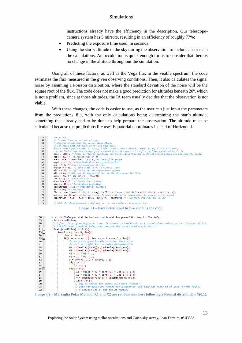
Image 3.1 – Parameter input before running the code.
Image 3.2 – Marsaglia Polar Method. X1 and X2 are random numbers following a Normal distribution N(0,1).
Simulations
14 Exploring the Solar System using stellar occultations and Gaia's sky survey, João Ferreira, nº 43363
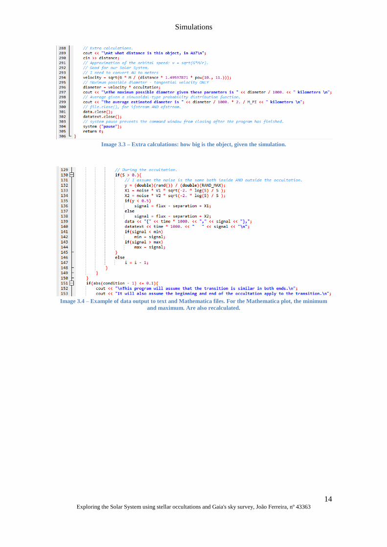
Image 3.3 – Extra calculations: how big is the object, given the simulation.
Image 3.4 – Example of data output to text and Mathematica files. For the Mathematica plot, the minimum
and maximum. Are also recalculated.
Regression
15 Exploring the Solar System using stellar occultations and Gaia's sky survey, João Ferreira, nº 43363
Chapter 4: Regression
After the simulation code was done, a new programming task was given: to create a
code that makes a regression for a stellar occultation. The function used for the regression is a
very specific one:
F = F0 − A ∗ HeavisidePi [t − t0
L]
Here, F is the calculated flux for a certain moment, t is the time, F0 the average flux of
the star, A the flux drop, t0 the median moment of the occultation and L the occultation’s duration.
HeavisidePi is a function defined as follows:
HeavisidePi(x) = {1, for |x| <
1
2
0, for |x| > 1
2
This regression gives us a constant flux with an instant drop and an identical instant rise
in arbitrary points in time. Without a transition phase for the occultation, this is the ideal case. If
done well, this regression shall indicate the most vital parameters of the event, namely how much
the flux drops compared to the signal noise and pinpointing when the occultation begins and ends.
During the first few months, a sketch of this regression was made using the software
Mathematica. However, the code usually diverged during the regression by the time the first
results had to be presented for the Traineeship. Still, the code included a set of calculations to
help determine reasonable initial values for the parameters, and it was decided to test these instead
of the regression itself. Despite this idea, one of the immediate downsides was that noise could
not be estimated.
Surprisingly, even though only initial approximations for the parameters were used, the
results were quite good. Using the simulator, the values to apply for each factor were under the
user´s control, and compared to the estimates of the regression code. The exposure time was once
again 0.25s. The result was an almost perfect determination of the time interval for the occultation,
in every case where it lasted over 2 seconds if the DNR of the flux drop was bigger than 3. For
flux drops smaller than that, but long occultations (> 10s), the test started to fail, but only deviated
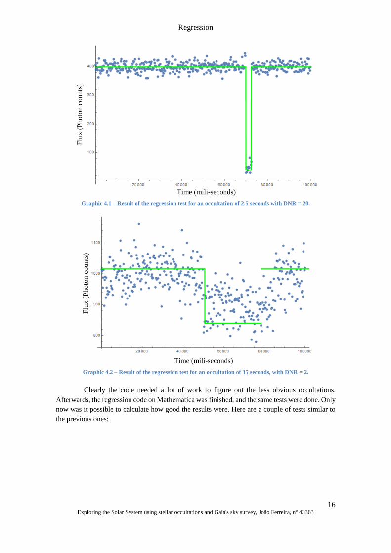
significantly from the observation when DNR < 2. A couple of results are shown in graphics 3
and 4:
Regression
16 Exploring the Solar System using stellar occultations and Gaia's sky survey, João Ferreira, nº 43363
Graphic 4.1 – Result of the regression test for an occultation of 2.5 seconds with DNR = 20.
Graphic 4.2 – Result of the regression test for an occultation of 35 seconds, with DNR = 2.
Clearly the code needed a lot of work to figure out the less obvious occultations.
Afterwards, the regression code on Mathematica was finished, and the same tests were done. Only
now was it possible to calculate how good the results were. Here are a couple of tests similar to
the previous ones:
Time (mili-seconds)
Flu
x (
Ph
oto
n c
oun
ts)
Time (mili-seconds)
Flu
x (
Photo
n c
ounts
)
Regression
17 Exploring the Solar System using stellar occultations and Gaia's sky survey, João Ferreira, nº 43363
Graphic 4.3 – Result of the regression test for an occultation of 2 seconds with DNR = 5.
Graphic 4.4 – Result of the regression test for an occultation of 25 seconds with DNR = 2.5.
For cases of DNR < 3, the code needed prior values to converge to acceptable results.
Nevertheless, the progress is clear, and a full statistical analysis was made, with the following
criteria:
• The parameters analyzed were the initial flux, the drop, the noise, the duration
and the beginning of the occultation. The DNR was also analyzed, but that is
just a combination of the drop and noise;
Regression
18 Exploring the Solar System using stellar occultations and Gaia's sky survey, João Ferreira, nº 43363
• The calculated parameters were compared with the input given to the simulation
code;
• The global results would determine whether the test was successful not.
Considering that, even with fixed input values, the output would not be exactly as what
the user set, there were three different classifications defined for the test results based on the
relative errors:
• Excellent, if every parameter had a relative error smaller than 10%;
• Very Good, if only one of them was greater than 10%;
• Good, if most were under 20%, and one was above;
• Reasonable, if most were above 20% and one or two were under;
• Failure, otherwise.
Once again, the exposure time was 0.25s. The tests were separated under 4 categories:
• Clear and long;
• Clear, but short;
• Faint and long;
• 2 seconds.
In the 2 seconds category, the DNR would gradually be decreased until the tests were
generally failures.
For clear (DNR > 10) and long (> 20s), the results were very good to excellent, as was
expected. This category had already been met with success with the previous approximation. The
code was particularly good at determining the duration and the initial flux, with the relative error
always being lower than 0.3%.
For clear, but short (< 5s), the results were similar to long occultations, except when the
duration reached 2 seconds (8 points inside the occultation), that being the reason it was separated
for a different analysis.
For faint (DNR < 5) and long, the results were very good until a DNR of 3 was reached.
For that value and DNR = 2.5, the tests were still reasonable, but for even smaller values they
were a failure, even with prior values given.
Occultations of 2 seconds were given a special focus. Professor Rui Agostinho
suggested a “zoom-in” was made on this occultation, using only 8x the amount of points outside
the occultation, both before and after. This way, the occultation would be easier to detect. Starting
with SNR = 50, going all the way down to SNR = 3, the results under these conditions were very
good to excellent for SNR ≥ 5, suggesting this sort of occultation can always be detected by the
code, and good for SNR ≥ 3, failing from that moment on.
Regression
19 Exploring the Solar System using stellar occultations and Gaia's sky survey, João Ferreira, nº 43363
Table 4.1 – Latest code tested for clear and long occultations.
Table 4.2 – Latest code tested for clear but short occultations.
Table 4.3 – Latest code tested for faint but long occultations.
Table 4.4 – Latest code tested for 2 second occultations.
A concise way of gathering this data is to plot the global error against a “figure of merit”,
which takes into account both the DNR and the amount of data points within the occultation:
Regression
20 Exploring the Solar System using stellar occultations and Gaia's sky survey, João Ferreira, nº 43363
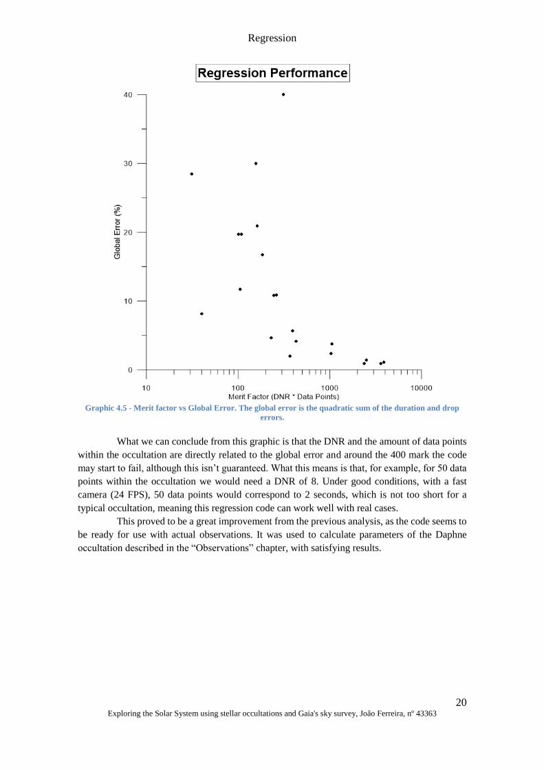
Graphic 4.5 - Merit factor vs Global Error. The global error is the quadratic sum of the duration and drop
errors.
What we can conclude from this graphic is that the DNR and the amount of data points
within the occultation are directly related to the global error and around the 400 mark the code
may start to fail, although this isn’t guaranteed. What this means is that, for example, for 50 data
points within the occultation we would need a DNR of 8. Under good conditions, with a fast
camera (24 FPS), 50 data points would correspond to 2 seconds, which is not too short for a
typical occultation, meaning this regression code can work well with real cases.
This proved to be a great improvement from the previous analysis, as the code seems to
be ready for use with actual observations. It was used to calculate parameters of the Daphne
occultation described in the “Observations” chapter, with satisfying results.
Regression
21 Exploring the Solar System using stellar occultations and Gaia's sky survey, João Ferreira, nº 43363
Image 4.1 – Initial part of the Mathematica code, where a brief description of the HeavisidePi function is
made, as well as knowing the amount of data.
Image 4.2 – Hand picking the initial values in case of a bad estimation by the code (hidden in comments
section) and building the regression function.
Image 4.3 – Statistical analysis of the regression's results for the occultation of Daphne.

Regression
22 Exploring the Solar System using stellar occultations and Gaia's sky survey, João Ferreira, nº 43363
Tangra – Data Reduction Software
23 Exploring the Solar System using stellar occultations and Gaia's sky survey, João Ferreira, nº 43363
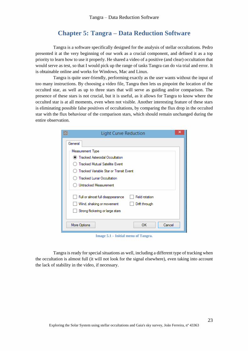
Chapter 5: Tangra – Data Reduction Software
Tangra is a software specifically designed for the analysis of stellar occultations. Pedro
presented it at the very beginning of our work as a crucial component, and defined it as a top
priority to learn how to use it properly. He shared a video of a positive (and clear) occultation that
would serve as test, so that I would pick up the range of tasks Tangra can do via trial and error. It
is obtainable online and works for Windows, Mac and Linux.
Tangra is quite user-friendly, performing exactly as the user wants without the input of
too many instructions. By choosing a video file, Tangra then lets us pinpoint the location of the
occulted star, as well as up to three stars that will serve as guiding and/or comparison. The
presence of these stars is not crucial, but it is useful, as it allows for Tangra to know where the
occulted star is at all moments, even when not visible. Another interesting feature of these stars
is eliminating possible false positives of occultations, by comparing the flux drop in the occulted
star with the flux behaviour of the comparison stars, which should remain unchanged during the
entire observation.
Image 5.1 – Initial menu of Tangra.
Tangra is ready for special situations as well, including a different type of tracking when
the occultation is almost full (it will not look for the signal elsewhere), even taking into account
the lack of stability in the video, if necessary.
Tangra – Data Reduction Software
24 Exploring the Solar System using stellar occultations and Gaia's sky survey, João Ferreira, nº 43363
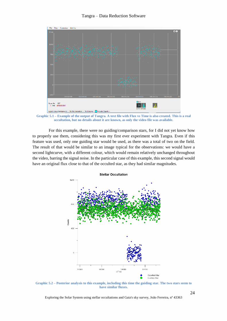
Graphic 5.1 – Example of the output of Tangra. A text file with Flux vs Time is also created. This is a real
occultation, but no details about it are known, as only the video file was available.
For this example, there were no guiding/comparison stars, for I did not yet know how
to properly use them, considering this was my first ever experiment with Tangra. Even if this
feature was used, only one guiding star would be used, as there was a total of two on the field.
The result of that would be similar to an image typical for the observations: we would have a
second lightcurve, with a different colour, which would remain relatively unchanged throughout
the video, barring the signal noise. In the particular case of this example, this second signal would
have an original flux close to that of the occulted star, as they had similar magnitudes.
Graphic 5.2 – Posterior analysis to this example, including this time the guiding star. The two stars seem to
have similar fluxes.
Tangra – Data Reduction Software
25 Exploring the Solar System using stellar occultations and Gaia's sky survey, João Ferreira, nº 43363
Recently, some changes have been made to Tangra with the release of a new version:
• The opening menu not only allows a choice on the type of event and the
observing conditions, but it can now also automatically integrate the video by
indicating the amount of frames to couple;
• Choosing the way of calculating the background, between the following:
o Average Background;
o Background Mode;
o 3D Polynomial Fit;
o PSF-Fitting Background;
o Median Background.
While all these methods have close average values throughout an entire
observation (as they should), and the video has the same time consumption, the
3D Polynomial Fit seems to be most stable one, with the smallest standard
deviation. For that reason, it was used instead of the others.
• Indicating if any filters were used (not relevant to the IA team’s observations,
as we do not use any).
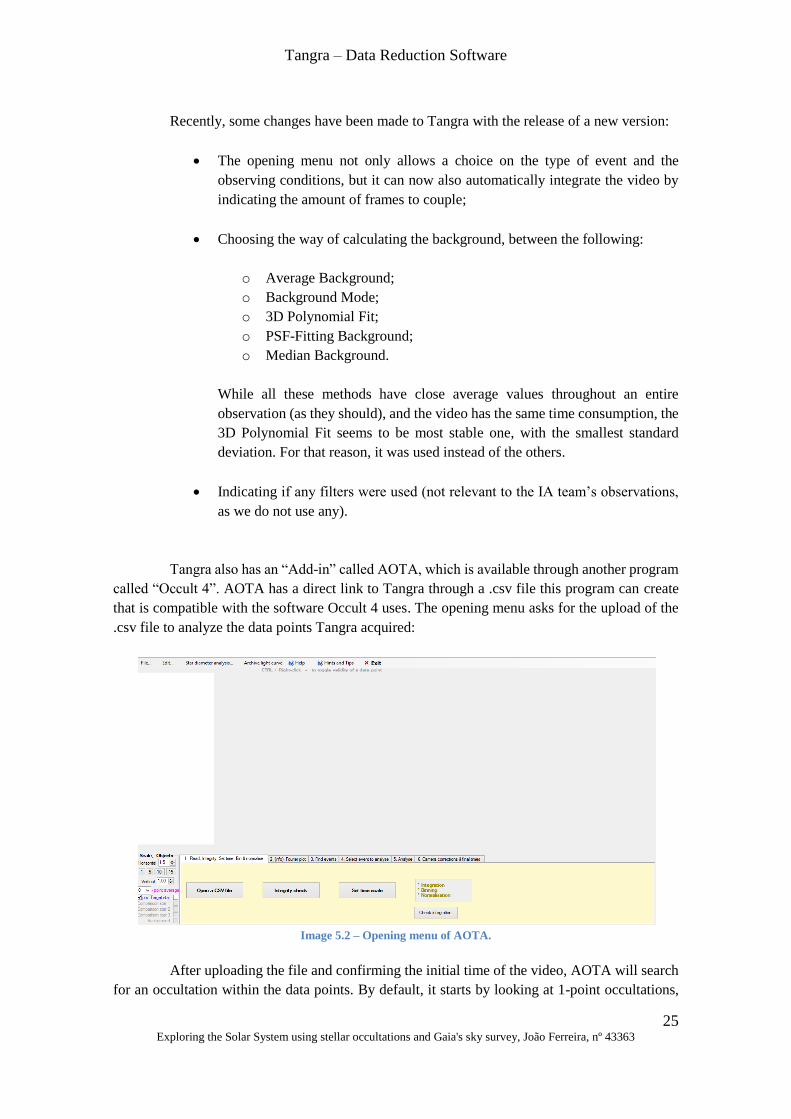
Tangra also has an “Add-in” called AOTA, which is available through another program
called “Occult 4”. AOTA has a direct link to Tangra through a .csv file this program can create
that is compatible with the software Occult 4 uses. The opening menu asks for the upload of the
.csv file to analyze the data points Tangra acquired:
Image 5.2 – Opening menu of AOTA.
After uploading the file and confirming the initial time of the video, AOTA will search
for an occultation within the data points. By default, it starts by looking at 1-point occultations,
Tangra – Data Reduction Software
26 Exploring the Solar System using stellar occultations and Gaia's sky survey, João Ferreira, nº 43363
and increase the number of points until a satisfactory result is reached. This can be quite time-
consuming, particularly for small amounts of points due to the signal noise, so it is best to give a
prior number of points within the occultation for AOTA to start with.
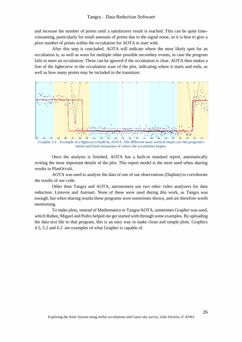
After this step is concluded, AOTA will indicate where the most likely spot for an
occultation is, as well as warn for multiple other possible secondary events, in case the program
fails to meet an occultation. These can be ignored if the occultation is clear. AOTA then makes a
line of the lightcurve in the occultation zone of the plot, indicating where it starts and ends, as
well as how many points may be included in the transition:
Graphic 5.3 – Example of a lightcurve built by AOTA. The different near-vertical slopes are the program's
initial and final estimation of where the occultation begins.
Once the analysis is finished, AOTA has a built-in standard report, automatically
writing the most important details of the plot. This report model is the most used when sharing
results in PlanOccult.
AOTA was used to analyze the data of one of our observations (Daphne) to corroborate
the results of our code.
Other than Tangra and AOTA, astronomers use two other video analyzers for data
reduction: Limovie and Astroart. None of these were used during this work, as Tangra was
enough, but when sharing results these programs were sometimes shown, and are therefore worth
mentioning.
To make plots, instead of Mathematica or Tangra/AOTA, sometimes Grapher was used,
which Ruben, Miguel and Pedro helped me get started with through some examples. By uploading
the data text file to that program, this is an easy way to make clean and simple plots. Graphics
4.5, 5.2 and 6.2 are examples of what Grapher is capable of.
Observations
27 Exploring the Solar System using stellar occultations and Gaia's sky survey, João Ferreira, nº 43363
Chapter 6: Observations
Parallel to this computational work, I also participated in four stellar occultation
observations during 2016. Three of these were made in Pedro’s house, at Troviscais (Alentejo),
while the other one was at Constância.
The criteria applied to choose a reasonable observation were the following:
• The star must have a magnitude no greater than 12.5, or our telescope might not
detect it;
• The star’s altitude at the moment of the occultation must be above 25º, or else
the atmosphere’s interference might be too strong;
• The Moon can’t be too close if it’s near the Full Moon Phase. No specific
angular distance is used, but preferably greater than 30º;
• The asteroid’s shadow path directly crosses Portugal. If only the uncertainty
region does, we do not consider it.
Besides all these factors, the team’s availability also played a role. With all these
constraints, four observations were planned and executed.
6.1: Psyche
In April 26th, our first observation was for the asteroid Psyche, which is located in the
asteroid belt between Mars and Jupiter. The standard procedure was laid out during the days prior
to the event:
• Use the software “Starry Night” (Pro Plus, 6th version) to see whether the
occulted star is visible in the hours prior to the occultation, for a potential lock
on the field ahead of time;
• Determine the FOV of the telescope;
• Print images of the predicted field of observation for the time of occultation.
We took the images from Starry Night with the following context: one would be the
camera’s FOV (11’x9’) and another one would have a maximum of 30’ for the smallest side of
the rectangle, as that was the size limit allowing us to take a picture. These would be asked inside
the program through an option named “LiveSky” with a sub-option “Show Photographic Image”.
This leads to the Starry Night webpage, giving us a photograph of the sky on that region.
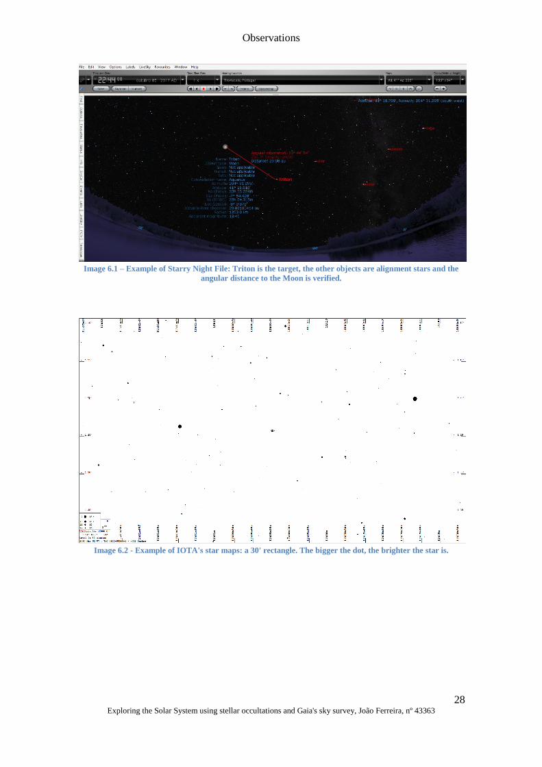
For bigger images, we use IOTA’s field maps, which include “Wide Field” (30ºx30º),
“15 degree View” (15ºx15º), and the same for 5º, 2º and 30’, all with the occulted star centred.
Observations
28 Exploring the Solar System using stellar occultations and Gaia's sky survey, João Ferreira, nº 43363
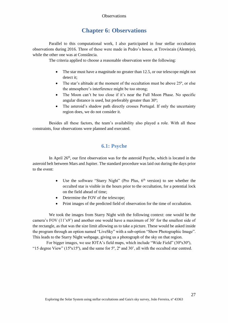
Image 6.1 – Example of Starry Night File: Triton is the target, the other objects are alignment stars and the
angular distance to the Moon is verified.
Image 6.2 - Example of IOTA's star maps: a 30' rectangle. The bigger the dot, the brighter the star is.
Observations
29 Exploring the Solar System using stellar occultations and Gaia's sky survey, João Ferreira, nº 43363
.
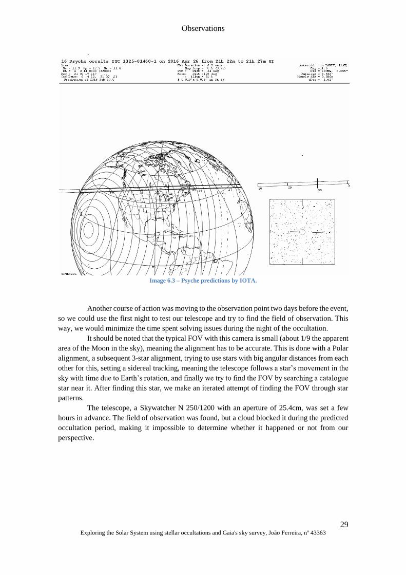
Image 6.3 – Psyche predictions by IOTA.
Another course of action was moving to the observation point two days before the event,
so we could use the first night to test our telescope and try to find the field of observation. This
way, we would minimize the time spent solving issues during the night of the occultation.
It should be noted that the typical FOV with this camera is small (about 1/9 the apparent
area of the Moon in the sky), meaning the alignment has to be accurate. This is done with a Polar
alignment, a subsequent 3-star alignment, trying to use stars with big angular distances from each
other for this, setting a sidereal tracking, meaning the telescope follows a star’s movement in the
sky with time due to Earth’s rotation, and finally we try to find the FOV by searching a catalogue
star near it. After finding this star, we make an iterated attempt of finding the FOV through star
patterns.
The telescope, a Skywatcher N 250/1200 with an aperture of 25.4cm, was set a few
hours in advance. The field of observation was found, but a cloud blocked it during the predicted
occultation period, making it impossible to determine whether it happened or not from our
perspective.
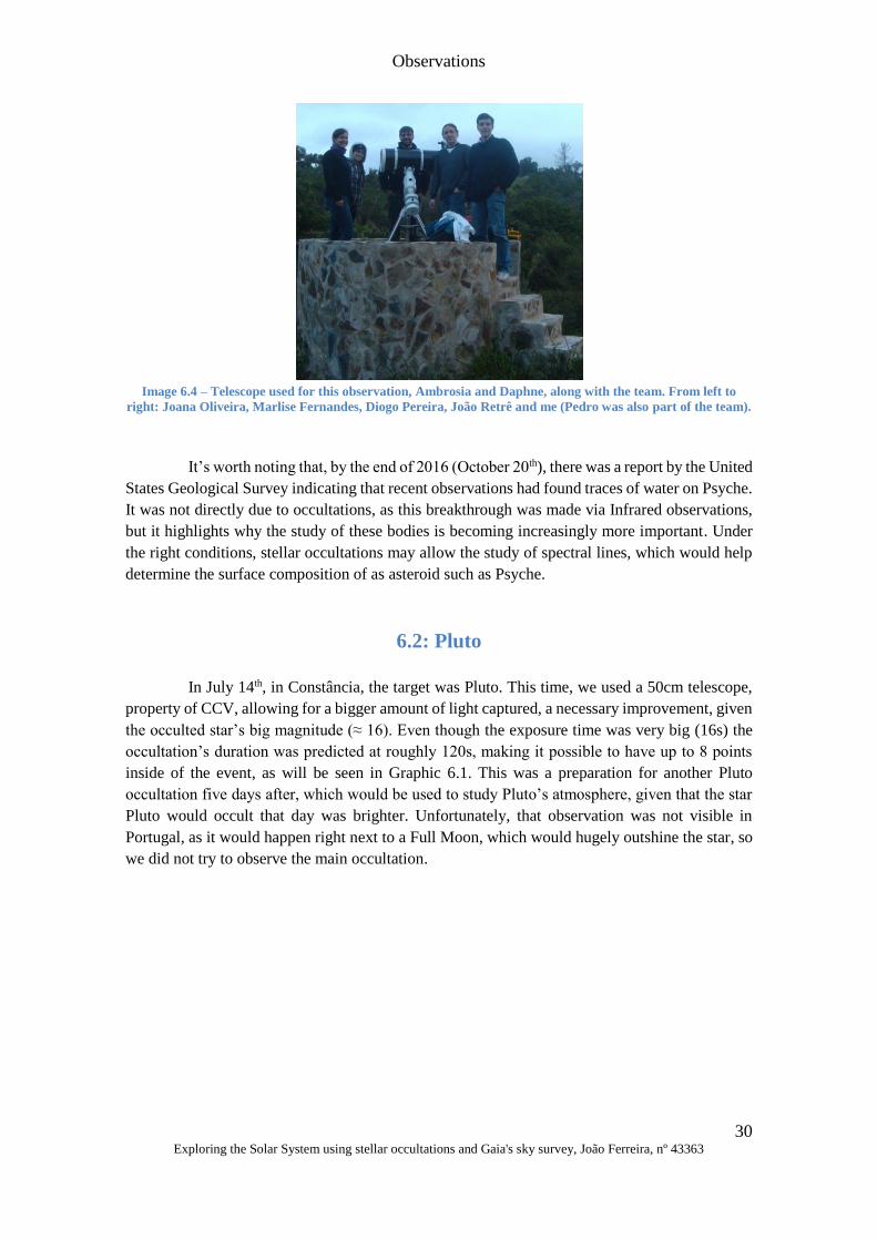
Observations
30 Exploring the Solar System using stellar occultations and Gaia's sky survey, João Ferreira, nº 43363
Image 6.4 – Telescope used for this observation, Ambrosia and Daphne, along with the team. From left to
right: Joana Oliveira, Marlise Fernandes, Diogo Pereira, João Retrê and me (Pedro was also part of the team).
It’s worth noting that, by the end of 2016 (October 20th), there was a report by the United
States Geological Survey indicating that recent observations had found traces of water on Psyche.
It was not directly due to occultations, as this breakthrough was made via Infrared observations,
but it highlights why the study of these bodies is becoming increasingly more important. Under
the right conditions, stellar occultations may allow the study of spectral lines, which would help
determine the surface composition of as asteroid such as Psyche.
6.2: Pluto
In July 14th, in Constância, the target was Pluto. This time, we used a 50cm telescope,
property of CCV, allowing for a bigger amount of light captured, a necessary improvement, given
the occulted star’s big magnitude (≈ 16). Even though the exposure time was very big (16s) the
occultation’s duration was predicted at roughly 120s, making it possible to have up to 8 points
inside of the event, as will be seen in Graphic 6.1. This was a preparation for another Pluto
occultation five days after, which would be used to study Pluto’s atmosphere, given that the star
Pluto would occult that day was brighter. Unfortunately, that observation was not visible in
Portugal, as it would happen right next to a Full Moon, which would hugely outshine the star, so
we did not try to observe the main occultation.
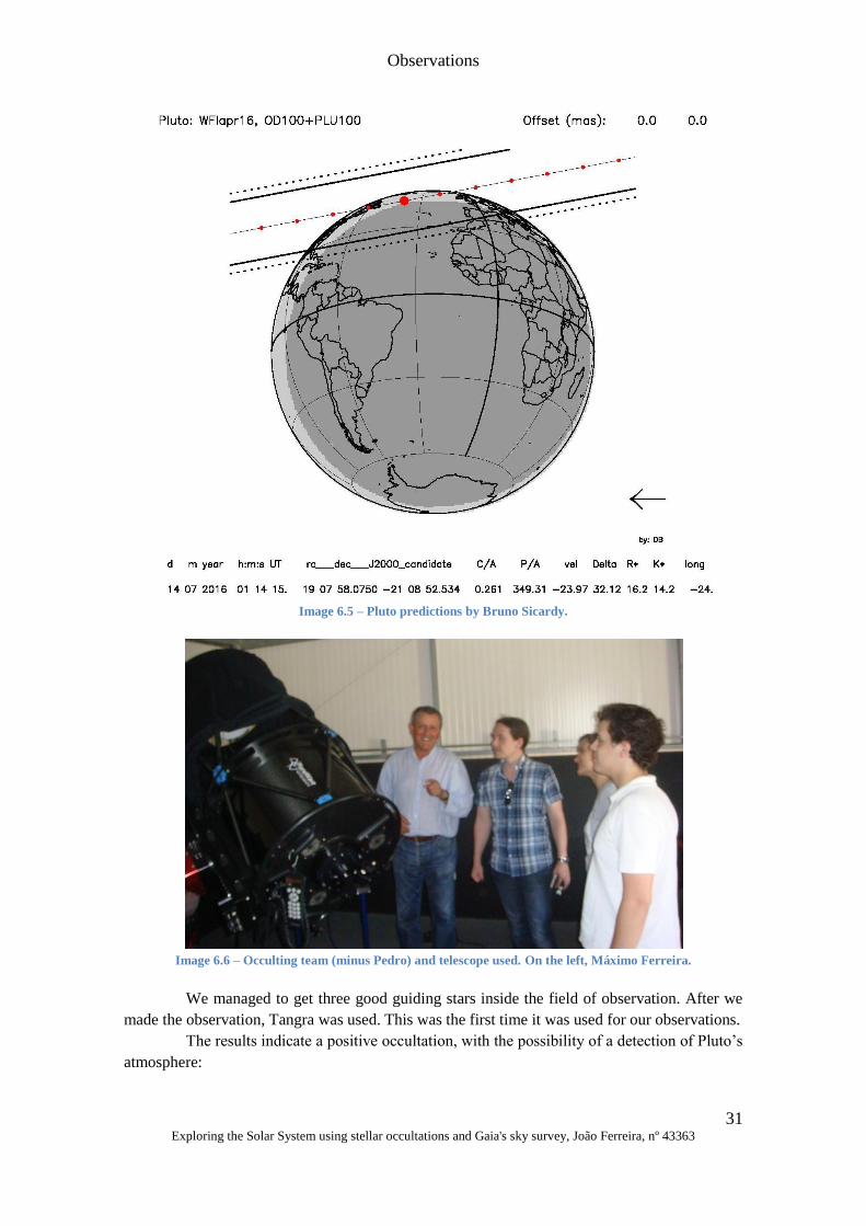
Observations
31 Exploring the Solar System using stellar occultations and Gaia's sky survey, João Ferreira, nº 43363
Image 6.5 – Pluto predictions by Bruno Sicardy.
Image 6.6 – Occulting team (minus Pedro) and telescope used. On the left, Máximo Ferreira.
We managed to get three good guiding stars inside the field of observation. After we
made the observation, Tangra was used. This was the first time it was used for our observations.
The results indicate a positive occultation, with the possibility of a detection of Pluto’s
atmosphere:
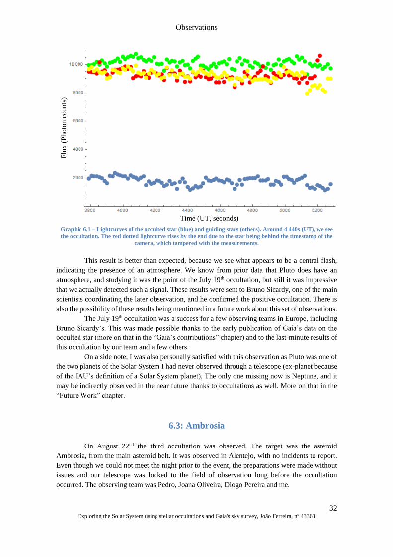
Observations
32 Exploring the Solar System using stellar occultations and Gaia's sky survey, João Ferreira, nº 43363
Graphic 6.1 – Lightcurves of the occulted star (blue) and guiding stars (others). Around 4 440s (UT), we see
the occultation. The red dotted lightcurve rises by the end due to the star being behind the timestamp of the
camera, which tampered with the measurements.
This result is better than expected, because we see what appears to be a central flash,
indicating the presence of an atmosphere. We know from prior data that Pluto does have an
atmosphere, and studying it was the point of the July 19th occultation, but still it was impressive
that we actually detected such a signal. These results were sent to Bruno Sicardy, one of the main
scientists coordinating the later observation, and he confirmed the positive occultation. There is
also the possibility of these results being mentioned in a future work about this set of observations.
The July 19th occultation was a success for a few observing teams in Europe, including
Bruno Sicardy’s. This was made possible thanks to the early publication of Gaia’s data on the
occulted star (more on that in the “Gaia’s contributions” chapter) and to the last-minute results of
this occultation by our team and a few others.
On a side note, I was also personally satisfied with this observation as Pluto was one of
the two planets of the Solar System I had never observed through a telescope (ex-planet because
of the IAU’s definition of a Solar System planet). The only one missing now is Neptune, and it
may be indirectly observed in the near future thanks to occultations as well. More on that in the
“Future Work” chapter.
6.3: Ambrosia
On August 22nd the third occultation was observed. The target was the asteroid
Ambrosia, from the main asteroid belt. It was observed in Alentejo, with no incidents to report.
Even though we could not meet the night prior to the event, the preparations were made without
issues and our telescope was locked to the field of observation long before the occultation
occurred. The observing team was Pedro, Joana Oliveira, Diogo Pereira and me.
Time (UT, seconds)
Flu
x (
Ph
oto
n c
oun
ts)
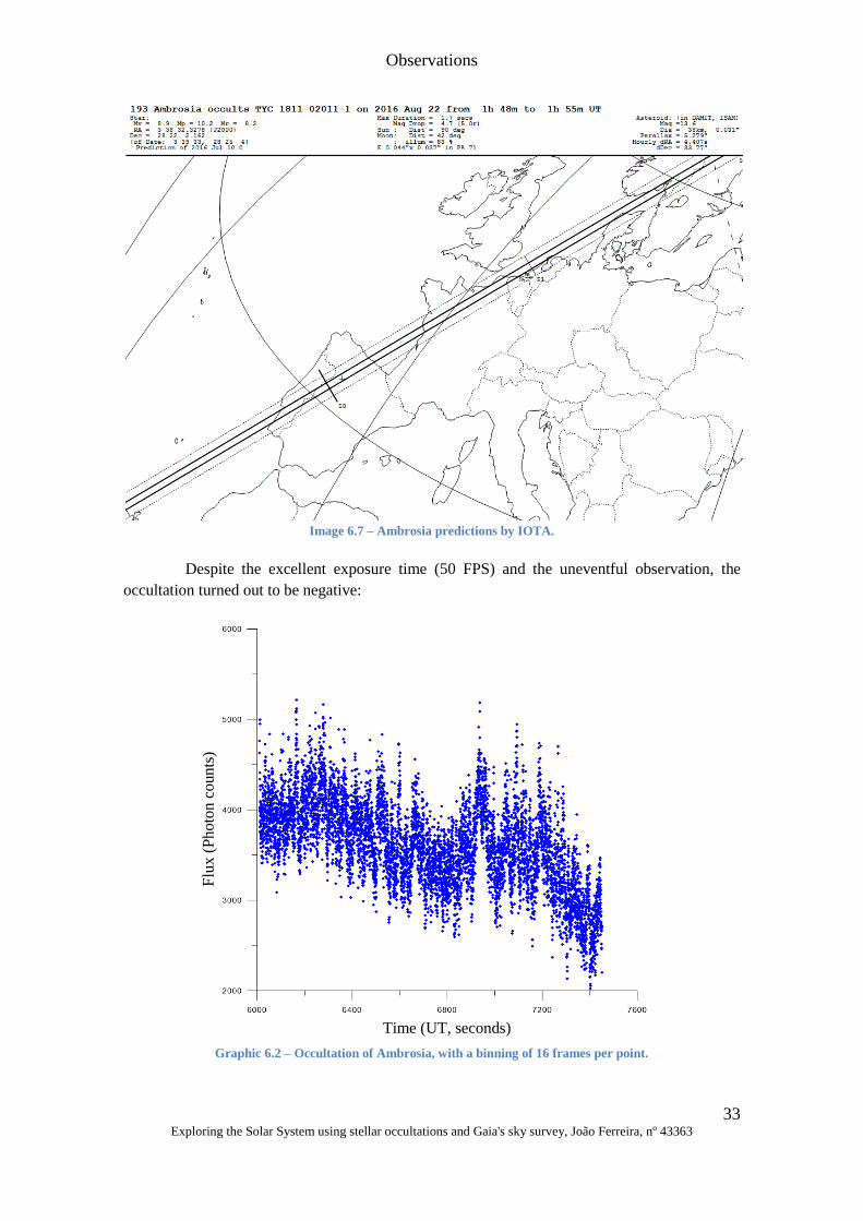
Observations
33 Exploring the Solar System using stellar occultations and Gaia's sky survey, João Ferreira, nº 43363
Image 6.7 – Ambrosia predictions by IOTA.
Despite the excellent exposure time (50 FPS) and the uneventful observation, the
occultation turned out to be negative:
Graphic 6.2 – Occultation of Ambrosia, with a binning of 16 frames per point.
Time (UT, seconds)
Flu
x (
Ph
oto
n c
oun
ts)
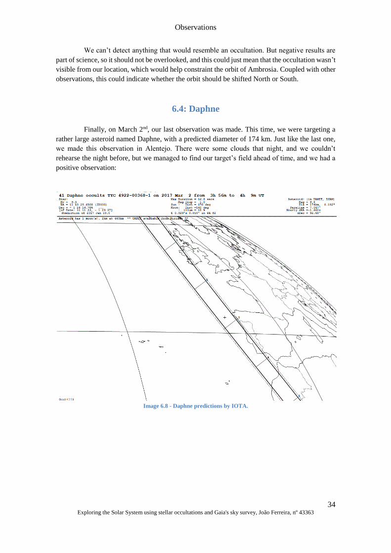
Observations
34 Exploring the Solar System using stellar occultations and Gaia's sky survey, João Ferreira, nº 43363
We can’t detect anything that would resemble an occultation. But negative results are
part of science, so it should not be overlooked, and this could just mean that the occultation wasn’t
visible from our location, which would help constraint the orbit of Ambrosia. Coupled with other
observations, this could indicate whether the orbit should be shifted North or South.
6.4: Daphne
Finally, on March 2nd, our last observation was made. This time, we were targeting a
rather large asteroid named Daphne, with a predicted diameter of 174 km. Just like the last one,
we made this observation in Alentejo. There were some clouds that night, and we couldn’t
rehearse the night before, but we managed to find our target’s field ahead of time, and we had a
positive observation:
Image 6.8 - Daphne predictions by IOTA.
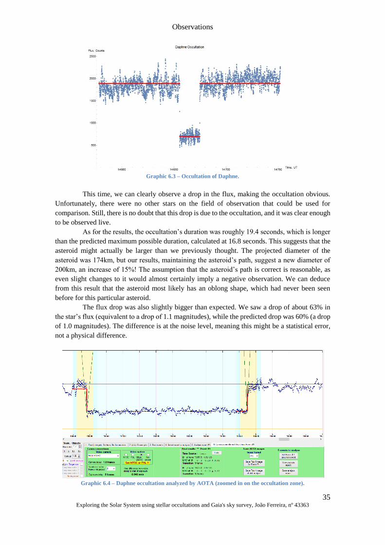
Observations
35 Exploring the Solar System using stellar occultations and Gaia's sky survey, João Ferreira, nº 43363
Graphic 6.3 – Occultation of Daphne.
This time, we can clearly observe a drop in the flux, making the occultation obvious.
Unfortunately, there were no other stars on the field of observation that could be used for
comparison. Still, there is no doubt that this drop is due to the occultation, and it was clear enough
to be observed live.
As for the results, the occultation’s duration was roughly 19.4 seconds, which is longer
than the predicted maximum possible duration, calculated at 16.8 seconds. This suggests that the
asteroid might actually be larger than we previously thought. The projected diameter of the
asteroid was 174km, but our results, maintaining the asteroid’s path, suggest a new diameter of
200km, an increase of 15%! The assumption that the asteroid’s path is correct is reasonable, as
even slight changes to it would almost certainly imply a negative observation. We can deduce
from this result that the asteroid most likely has an oblong shape, which had never been seen
before for this particular asteroid.
The flux drop was also slightly bigger than expected. We saw a drop of about 63% in
the star’s flux (equivalent to a drop of 1.1 magnitudes), while the predicted drop was 60% (a drop
of 1.0 magnitudes). The difference is at the noise level, meaning this might be a statistical error,
not a physical difference.
Graphic 6.4 – Daphne occultation analyzed by AOTA (zoomed in on the occultation zone).
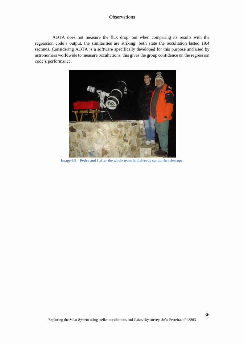
Observations
36 Exploring the Solar System using stellar occultations and Gaia's sky survey, João Ferreira, nº 43363
AOTA does not measure the flux drop, but when comparing its results with the
regression code’s output, the similarities are striking: both state the occultation lasted 19.4
seconds. Considering AOTA is a software specifically developed for this purpose and used by
astronomers worldwide to measure occultations, this gives the group confidence on the regression
code’s performance.
Image 6.9 – Pedro and I after the whole team had already set up the telescope.
PlanOccult Results
37 Exploring the Solar System using stellar occultations and Gaia's sky survey, João Ferreira, nº 43363
Chapter 7: PlanOccult Results
PlanOccult is an asteroid occultation mailing list, though it may also be used for TNO
and planetary occultations as well. Anyone can join this list, and astronomers from all around the
world can cooperate by sharing their results. I joined this list in early October 2016, and since
then received several messages reporting occultations, mainly in Europe and the US. This not
only allows a study on the typical analysis of both positive and negative observations, but also
makes it possible to keeps up to date with the current research on the field. It also gives a good
statistic of how often occultations are positive and how many observations of this kind are made
worldwide.
Since joining PlanOccult, there have been 92 positive and about 960 negative
occultations, for about 1050 observations in nine months. This means that over 100 observations
on this topic are made each month, and that even with current predictions for these events, the
odds of it being positive are low (about 1 in 11). This amount of negative events can be due to
two main reasons (other than bad weather, which results in no observation rather than a negative):
• The observation was inadequate for the event. This might happen if the
occultation is either too faint or too fast for the equipment used, or if the star
occulted is itself too faint, which may happen often for automated
observatories;
• The prediction was inaccurate in the shadow path projection, meaning the
asteroid’s orbit was different from the one catalogues suggested, or the star was
slightly deviated from its predicted position.
The first point can only be solved with good planning, which the IA team is fully capable
of. There is always a conscious choice of both the event and the observatory depending on the
predicted conditions, so that this may never be an issue.
As for the second point, only through experience can we diminish its effect. The better
we know the orbits of asteroids and the positions of the stars, the less we will be exposed to this
risk. That is the reason why Gaia is so important: the uncertainty on the position of many of the
occulted stars will be drastically smaller. A few orbits of asteroids will also be studied with Gaia,
but the biggest effect will be on the stars’ positions.
PlanOccult was directly useful thanks to their help in installing Occult 4 and getting
started with it via examples. Some of the members of this mailing list are also responsible for
most of the updates made to that software.
The main positive asteroid results shared in PlanOccult throughout the last year were:
• Kalliope (estimated diameter: 235 km), observed by at least three
independent observatories in Czech Republic and Italy on November 8th;
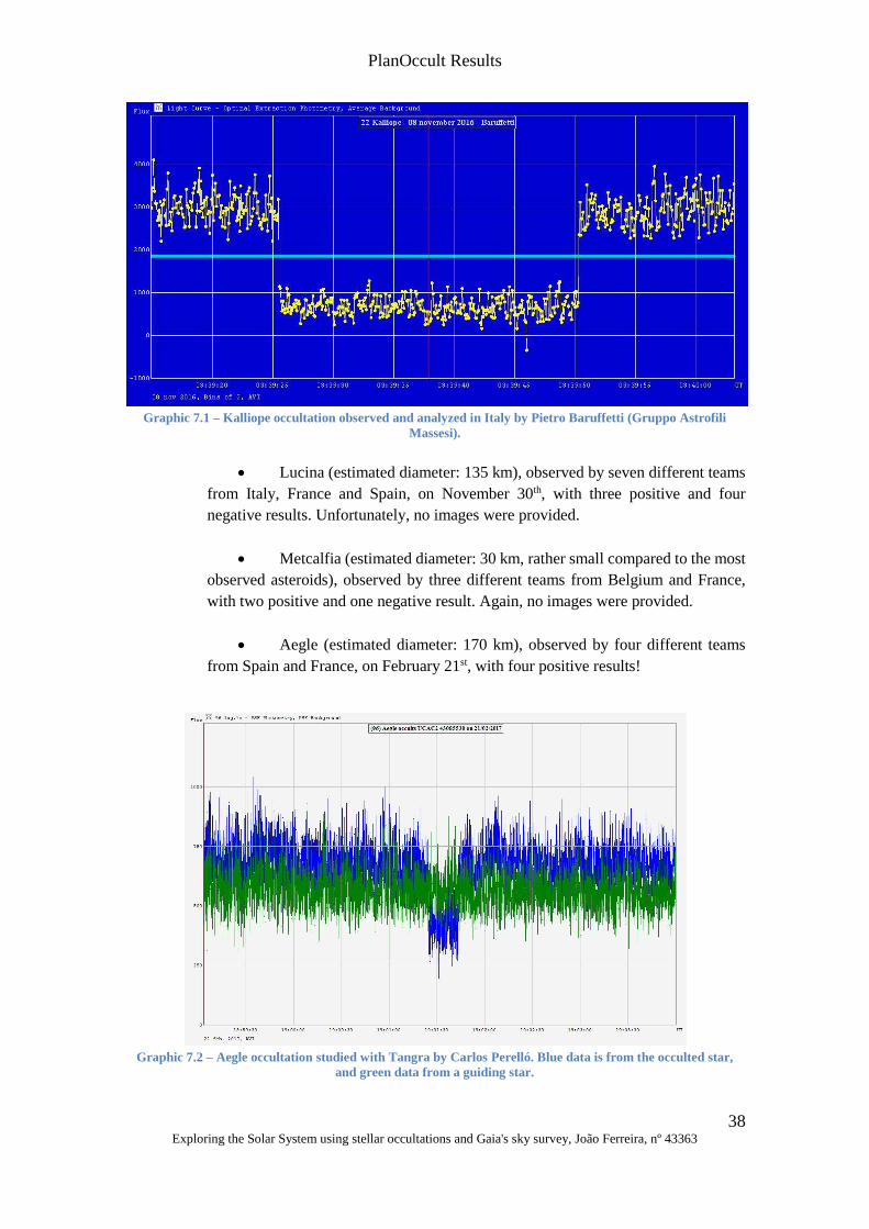
PlanOccult Results
38 Exploring the Solar System using stellar occultations and Gaia's sky survey, João Ferreira, nº 43363
Graphic 7.1 – Kalliope occultation observed and analyzed in Italy by Pietro Baruffetti (Gruppo Astrofili
Massesi).
• Lucina (estimated diameter: 135 km), observed by seven different teams
from Italy, France and Spain, on November 30th, with three positive and four
negative results. Unfortunately, no images were provided.
• Metcalfia (estimated diameter: 30 km, rather small compared to the most
observed asteroids), observed by three different teams from Belgium and France,
with two positive and one negative result. Again, no images were provided.
• Aegle (estimated diameter: 170 km), observed by four different teams
from Spain and France, on February 21st, with four positive results!
Graphic 7.2 – Aegle occultation studied with Tangra by Carlos Perelló. Blue data is from the occulted star,
and green data from a guiding star.
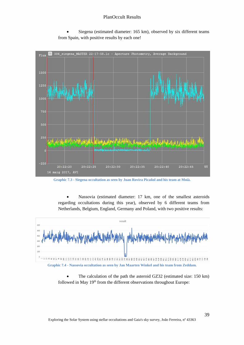
PlanOccult Results
39 Exploring the Solar System using stellar occultations and Gaia's sky survey, João Ferreira, nº 43363
• Siegena (estimated diameter: 165 km), observed by six different teams
from Spain, with positive results by each one!
Graphic 7.3 - Siegena occultation as seen by Juan Rovira Picañol and his team at Moià.
• Nassovia (estimated diameter: 17 km, one of the smallest asteroids
regarding occultations during this year), observed by 6 different teams from
Netherlands, Belgium, England, Germany and Poland, with two positive results:
Graphic 7.4 - Nassovia occultation as seen by Jan Maarten Winkel and his team from Zeddam.
• The calculation of the path the asteroid GZ32 (estimated size: 150 km)
followed in May 19th from the different observations throughout Europe:
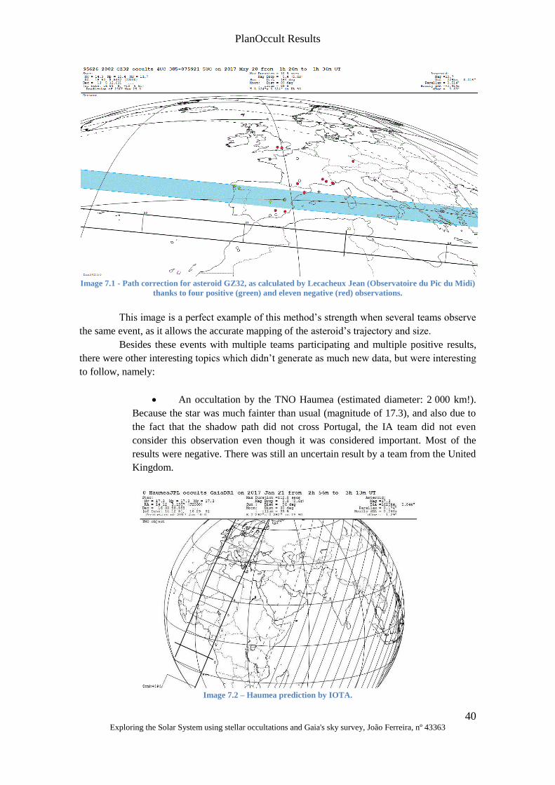
PlanOccult Results
40 Exploring the Solar System using stellar occultations and Gaia's sky survey, João Ferreira, nº 43363
Image 7.1 - Path correction for asteroid GZ32, as calculated by Lecacheux Jean (Observatoire du Pic du Midi)
thanks to four positive (green) and eleven negative (red) observations.
This image is a perfect example of this method’s strength when several teams observe
the same event, as it allows the accurate mapping of the asteroid’s trajectory and size.
Besides these events with multiple teams participating and multiple positive results,
there were other interesting topics which didn’t generate as much new data, but were interesting
to follow, namely:
• An occultation by the TNO Haumea (estimated diameter: 2 000 km!).
Because the star was much fainter than usual (magnitude of 17.3), and also due to
the fact that the shadow path did not cross Portugal, the IA team did not even
consider this observation even though it was considered important. Most of the
results were negative. There was still an uncertain result by a team from the United
Kingdom.
Image 7.2 – Haumea prediction by IOTA.
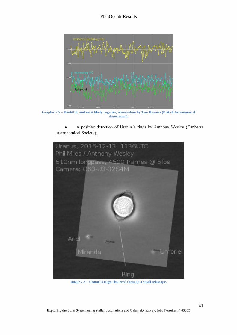
PlanOccult Results
41 Exploring the Solar System using stellar occultations and Gaia's sky survey, João Ferreira, nº 43363
Graphic 7.5 – Doubtful, and most likely negative, observation by Tim Haymes (British Astronomical
Association).
• A positive detection of Uranus’s rings by Anthony Wesley (Canberra
Astronomical Society).
Image 7.3 – Uranus’s rings observed through a small telescope.
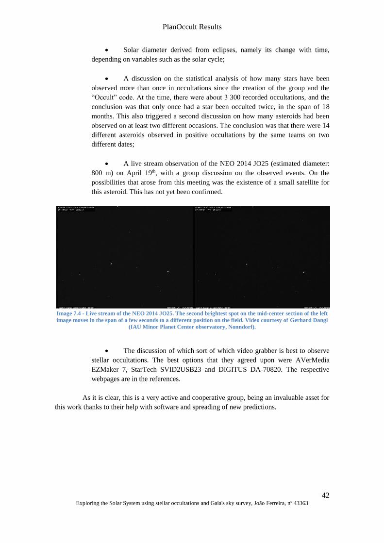
PlanOccult Results
42 Exploring the Solar System using stellar occultations and Gaia's sky survey, João Ferreira, nº 43363
• Solar diameter derived from eclipses, namely its change with time,
depending on variables such as the solar cycle;
• A discussion on the statistical analysis of how many stars have been
observed more than once in occultations since the creation of the group and the
“Occult” code. At the time, there were about 3 300 recorded occultations, and the
conclusion was that only once had a star been occulted twice, in the span of 18
months. This also triggered a second discussion on how many asteroids had been
observed on at least two different occasions. The conclusion was that there were 14
different asteroids observed in positive occultations by the same teams on two
different dates;
• A live stream observation of the NEO 2014 JO25 (estimated diameter:
800 m) on April 19th, with a group discussion on the observed events. On the
possibilities that arose from this meeting was the existence of a small satellite for
this asteroid. This has not yet been confirmed.
Image 7.4 - Live stream of the NEO 2014 JO25. The second brightest spot on the mid-center section of the left
image moves in the span of a few seconds to a different position on the field. Video courtesy of Gerhard Dangl
(IAU Minor Planet Center observatory, Nonndorf).
• The discussion of which sort of which video grabber is best to observe
stellar occultations. The best options that they agreed upon were AVerMedia
EZMaker 7, StarTech SVID2USB23 and DIGITUS DA-70820. The respective
webpages are in the references.
As it is clear, this is a very active and cooperative group, being an invaluable asset for
this work thanks to their help with software and spreading of new predictions.
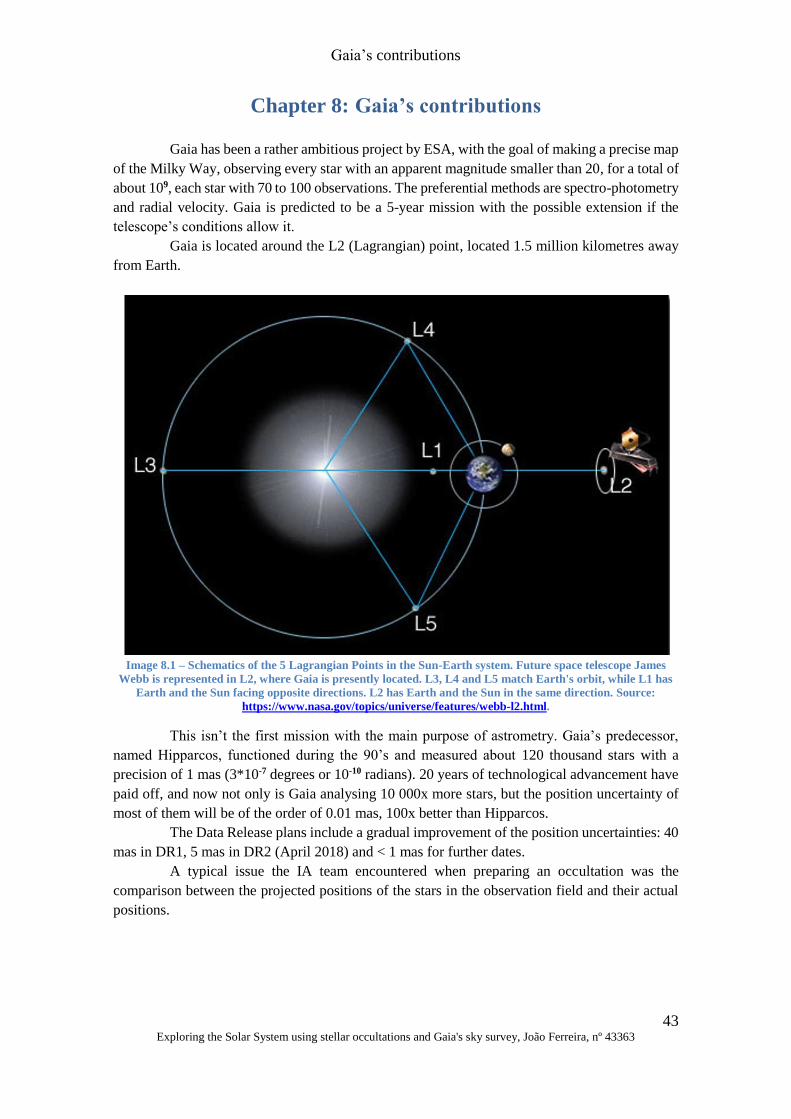
Gaia’s contributions
43 Exploring the Solar System using stellar occultations and Gaia's sky survey, João Ferreira, nº 43363
Chapter 8: Gaia’s contributions
Gaia has been a rather ambitious project by ESA, with the goal of making a precise map
of the Milky Way, observing every star with an apparent magnitude smaller than 20, for a total of
about 109, each star with 70 to 100 observations. The preferential methods are spectro-photometry
and radial velocity. Gaia is predicted to be a 5-year mission with the possible extension if the
telescope’s conditions allow it.
Gaia is located around the L2 (Lagrangian) point, located 1.5 million kilometres away
from Earth.
Image 8.1 – Schematics of the 5 Lagrangian Points in the Sun-Earth system. Future space telescope James
Webb is represented in L2, where Gaia is presently located. L3, L4 and L5 match Earth's orbit, while L1 has
Earth and the Sun facing opposite directions. L2 has Earth and the Sun in the same direction. Source:
https://www.nasa.gov/topics/universe/features/webb-l2.html.
This isn’t the first mission with the main purpose of astrometry. Gaia’s predecessor,
named Hipparcos, functioned during the 90’s and measured about 120 thousand stars with a
precision of 1 mas (3*10-7 degrees or 10-10 radians). 20 years of technological advancement have
paid off, and now not only is Gaia analysing 10 000x more stars, but the position uncertainty of
most of them will be of the order of 0.01 mas, 100x better than Hipparcos.
The Data Release plans include a gradual improvement of the position uncertainties: 40
mas in DR1, 5 mas in DR2 (April 2018) and < 1 mas for further dates.
A typical issue the IA team encountered when preparing an occultation was the
comparison between the projected positions of the stars in the observation field and their actual
positions.
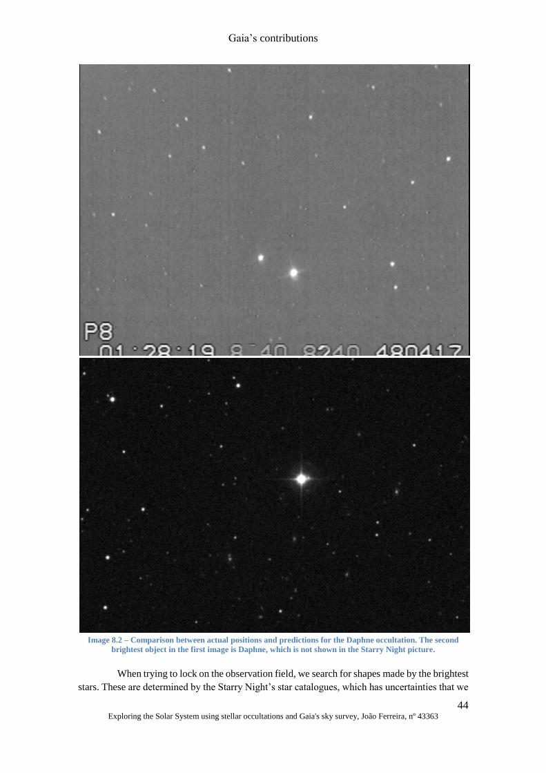
Gaia’s contributions
44 Exploring the Solar System using stellar occultations and Gaia's sky survey, João Ferreira, nº 43363
Image 8.2 – Comparison between actual positions and predictions for the Daphne occultation. The second
brightest object in the first image is Daphne, which is not shown in the Starry Night picture.
When trying to lock on the observation field, we search for shapes made by the brightest
stars. These are determined by the Starry Night’s star catalogues, which has uncertainties that we
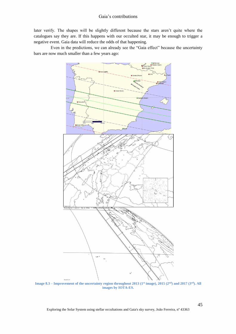
Gaia’s contributions
45 Exploring the Solar System using stellar occultations and Gaia's sky survey, João Ferreira, nº 43363
later verify. The shapes will be slightly different because the stars aren’t quite where the
catalogues say they are. If this happens with our occulted star, it may be enough to trigger a
negative event. Gaia data will reduce the odds of that happening.
Even in the predictions, we can already see the “Gaia effect” because the uncertainty
bars are now much smaller than a few years ago:
Image 8.3 – Improvement of the uncertainty region throughout 2013 (1st image), 2015 (2nd) and 2017 (3rd). All
images by IOTA-ES.
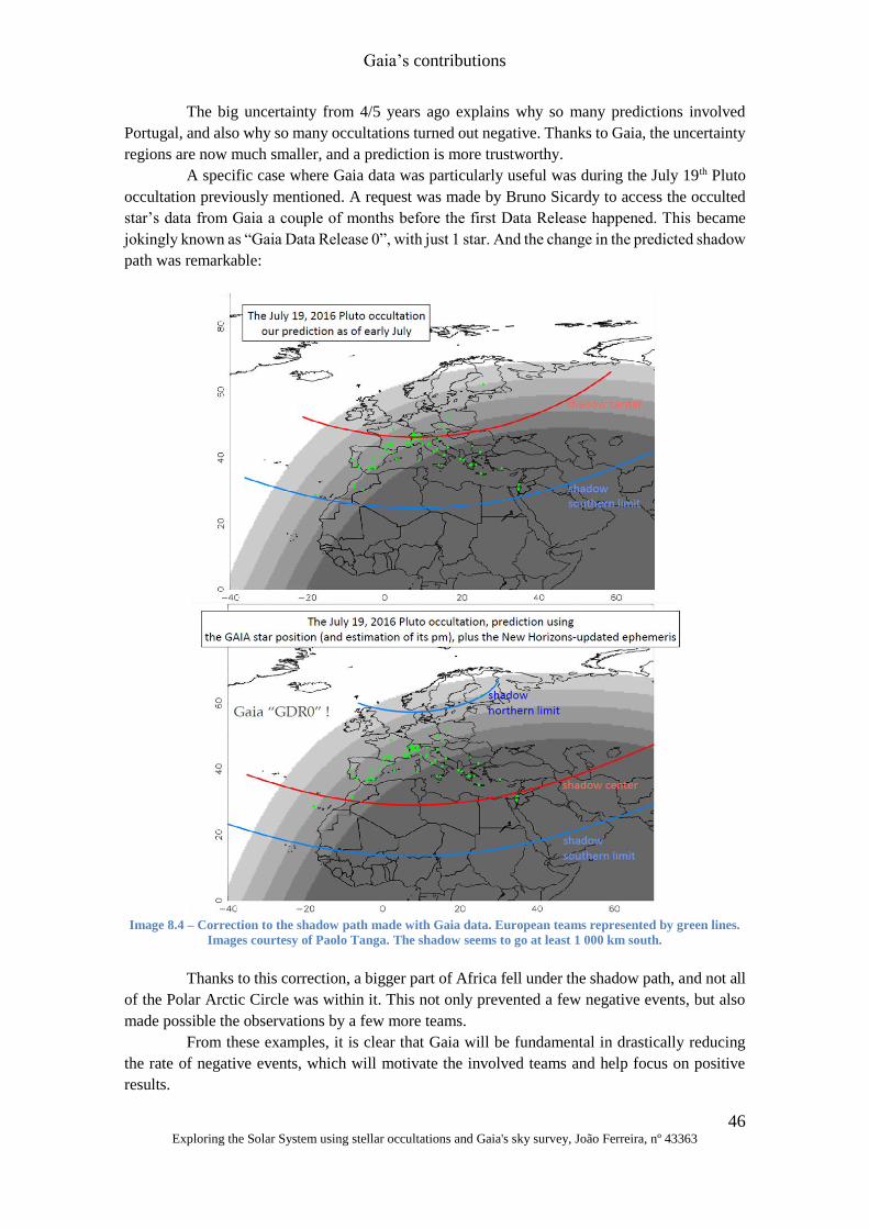
Gaia’s contributions
46 Exploring the Solar System using stellar occultations and Gaia's sky survey, João Ferreira, nº 43363
The big uncertainty from 4/5 years ago explains why so many predictions involved
Portugal, and also why so many occultations turned out negative. Thanks to Gaia, the uncertainty
regions are now much smaller, and a prediction is more trustworthy.
A specific case where Gaia data was particularly useful was during the July 19th Pluto
occultation previously mentioned. A request was made by Bruno Sicardy to access the occulted
star’s data from Gaia a couple of months before the first Data Release happened. This became
jokingly known as “Gaia Data Release 0”, with just 1 star. And the change in the predicted shadow
path was remarkable:
Image 8.4 – Correction to the shadow path made with Gaia data. European teams represented by green lines.
Images courtesy of Paolo Tanga. The shadow seems to go at least 1 000 km south.
Thanks to this correction, a bigger part of Africa fell under the shadow path, and not all
of the Polar Arctic Circle was within it. This not only prevented a few negative events, but also
made possible the observations by a few more teams.
From these examples, it is clear that Gaia will be fundamental in drastically reducing
the rate of negative events, which will motivate the involved teams and help focus on positive
results.
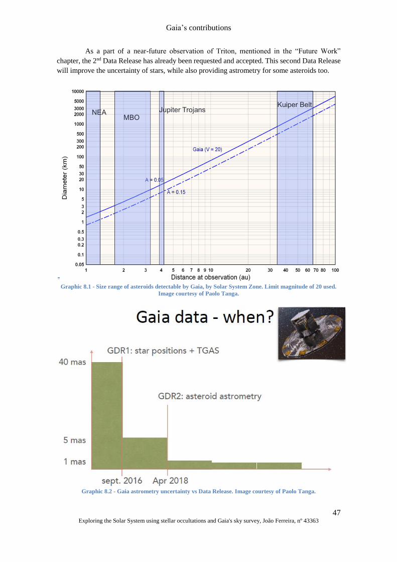
Gaia’s contributions
47 Exploring the Solar System using stellar occultations and Gaia's sky survey, João Ferreira, nº 43363
As a part of a near-future observation of Triton, mentioned in the “Future Work”
chapter, the 2nd Data Release has already been requested and accepted. This second Data Release
will improve the uncertainty of stars, while also providing astrometry for some asteroids too.
Graphic 8.1 - Size range of asteroids detectable by Gaia, by Solar System Zone. Limit magnitude of 20 used.
Image courtesy of Paolo Tanga.
Graphic 8.2 - Gaia astrometry uncertainty vs Data Release. Image courtesy of Paolo Tanga.

Gaia’s contributions
48 Exploring the Solar System using stellar occultations and Gaia's sky survey, João Ferreira, nº 43363
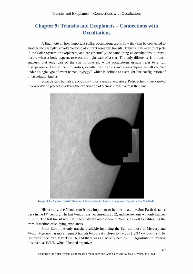
Transits and Exoplanets – Connections with Occultations
49 Exploring the Solar System using stellar occultations and Gaia's sky survey, João Ferreira, nº 43363
Chapter 9: Transits and Exoplanets – Connections with
Occultations
A final note on how important stellar occultations are is how they can be connected to
another increasingly remarkable topic of current research: transits. Transits may refer to objects
in the Solar System or exoplanets, and are essentially the same thing as occultations: a transit
occurs when a body appears to cross the light path of a star. The only difference is a transit
suggests that only part of the star is covered, while occultations usually refer to a full
disappearance. Due to the similarities, occultations, transits and even eclipses are all coupled
under a single type of event named “syzygy”, which is defined as a straight-line configuration of
three celestial bodies.
Solar System transits are one of my tutor’s areas of expertise. Pedro actually participated
in a worldwide project involving the observation of Venus’s transit across the Sun:
Image 9.1 – Venus transit. This event lasted about 6 hours. Image courtesy of Pedro Machado.
Historically, the Venus transit was important to help estimate the Sun-Earth distance
back in the 17th century. The last Venus transit occurred in 2012, and the next one will only happen
in 2117. The last transit was useful to study the atmosphere of Venus, as well as calibrating the
transits method of studying exoplanets.
From Earth, the only transits available involving the Sun are those of Mercury and
Venus. Mercury has more frequent transits because it’s closer to the Sun (13/14 each century). Its
last transit occurred May 9th 2016, and there was an activity held by Rui Agostinho to observe
this event at FCUL, which I helped organize:
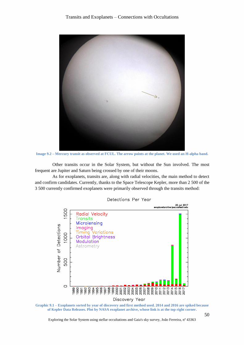
Transits and Exoplanets – Connections with Occultations
50 Exploring the Solar System using stellar occultations and Gaia's sky survey, João Ferreira, nº 43363
Image 9.2 – Mercury transit as observed at FCUL. The arrow points at the planet. We used an H-alpha band.
Other transits occur in the Solar System, but without the Sun involved. The most
frequent are Jupiter and Saturn being crossed by one of their moons.
As for exoplanets, transits are, along with radial velocities, the main method to detect
and confirm candidates. Currently, thanks to the Space Telescope Kepler, more than 2 500 of the
3 500 currently confirmed exoplanets were primarily observed through the transits method:
Graphic 9.1 – Exoplanets sorted by year of discovery and first method used. 2014 and 2016 are spiked because
of Kepler Data Releases. Plot by NASA exoplanet archive, whose link is at the top right corner.
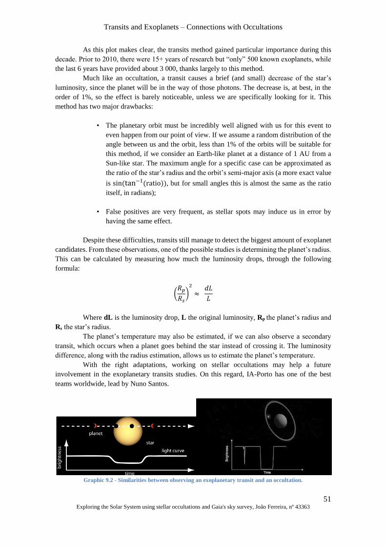
Transits and Exoplanets – Connections with Occultations
51 Exploring the Solar System using stellar occultations and Gaia's sky survey, João Ferreira, nº 43363
As this plot makes clear, the transits method gained particular importance during this
decade. Prior to 2010, there were 15+ years of research but “only” 500 known exoplanets, while
the last 6 years have provided about 3 000, thanks largely to this method.
Much like an occultation, a transit causes a brief (and small) decrease of the star’s
luminosity, since the planet will be in the way of those photons. The decrease is, at best, in the
order of 1%, so the effect is barely noticeable, unless we are specifically looking for it. This
method has two major drawbacks:
• The planetary orbit must be incredibly well aligned with us for this event to
even happen from our point of view. If we assume a random distribution of the
angle between us and the orbit, less than 1% of the orbits will be suitable for
this method, if we consider an Earth-like planet at a distance of 1 AU from a
Sun-like star. The maximum angle for a specific case can be approximated as
the ratio of the star’s radius and the orbit’s semi-major axis (a more exact value
is sin (tan−1(ratio)), but for small angles this is almost the same as the ratio
itself, in radians);
• False positives are very frequent, as stellar spots may induce us in error by
having the same effect.
Despite these difficulties, transits still manage to detect the biggest amount of exoplanet
candidates. From these observations, one of the possible studies is determining the planet’s radius.
This can be calculated by measuring how much the luminosity drops, through the following
formula:
(𝑅𝑝
𝑅𝑠)
2
≈ 𝑑𝐿
𝐿
Where dL is the luminosity drop, L the original luminosity, Rp the planet’s radius and
Rs the star’s radius.
The planet’s temperature may also be estimated, if we can also observe a secondary
transit, which occurs when a planet goes behind the star instead of crossing it. The luminosity
difference, along with the radius estimation, allows us to estimate the planet’s temperature.
With the right adaptations, working on stellar occultations may help a future
involvement in the exoplanetary transits studies. On this regard, IA-Porto has one of the best
teams worldwide, lead by Nuno Santos.
Graphic 9.2 - Similarities between observing an exoplanetary transit and an occultation.
Transits and Exoplanets – Connections with Occultations
52 Exploring the Solar System using stellar occultations and Gaia's sky survey, João Ferreira, nº 43363
Conclusions
53 Exploring the Solar System using stellar occultations and Gaia's sky survey, João Ferreira, nº 43363
Chapter 10: Conclusions
Despite being a recent method of Solar System study, just now beginning to gain a
critical mass of both predictions and observations, stellar occultations have already allowed a
better understanding of small bodies, fundamental to the knowledge of a planetary system’s
formation process. Asteroids and TNO, like Pluto, Makemake and Eris, have seen major
breakthroughs in their studies thanks to the worldwide efforts of astronomers under this type of
observation.
Even though I am new to this field, I always felt part of a group thanks to the constant
support by Pedro and Paolo.
The four occultation observations allowed me to gain valuable experience for the future,
making me aware of the specifics this type of event requires, as well as preparing me to the most
common issues. The fact that two positive occultations were possible, one from a far away object
like Pluto shows that our group is solid and ready for the next challenges.
The Psyche observation was a failure due to a misfortune. Ambrosia, in spite of the
predicted shadow path, turned out to be negative. Given the predicted conditions (a 99% drop on
the flux, and an 8.9 magnitude star), the most likely explanation was a bad calculation of the
asteroid’s path. Looking at the uncertainty region, it is actually bigger than the shadow region,
which is why such an occurrence might have happened.
The Daphne occultation was a success, as it was the first independent observation of
this kind by the IA team to have positive results. Prior to this, the only positive occultation we
had observed was requested by Bruno Sicardy. This was also decisive to demonstrate the team’s
importance and ability of contributing on this field.
Also about the Daphne occultations, our results were surprising, suggesting that this
asteroid is bigger than we thought. If our estimated diameter is correct (≈ 200km), Daphne would
move up on the list of the largest asteroids, and its mass, currently estimated at 7*1018 kg, would
probably increase as well.
After meeting with Paolo, the simulations code was adapted to better suit our
expectations. Now, it is simpler to read, quicker to use, and several simulations can be made
instead of just one, allowing a statistical analysis of the limit-cases of the regression code (faint
and/or short occultations).
The regression code is ready for clear and/or long occultations. It can determine to a
good degree the physical parameters of the object involved in the simulation or the observation,
and has withstood a test against a tool used by most astronomers in this field, Occult 4, by not
only matching the occultation’s beginning and duration, but even going further, calculating the
flux drop and the noise.
Tangra was useful throughout this project, providing a simple connection between the
video files and text files, and creating files that Occult 4 can support. These two programs, when
combined, allow a complete study on any observation made, and have built-in report files that we
can send to every astronomer linked to PlanOccult. PlanOccult has shown me that stellar
occultations are increasingly important, both in number of astronomers and information
processed. Groups from different regions plan joint observations for particular events, allowing a
better study of the object. This was made with Pluto, Haumea and is now being planned for Triton.
More on that in the “Future Work” chapter.
Gaia has slowly started to show up in IOTA’s predictions. This means we should expect
an increase in the positive-to-negative observations ratio, which will both motivate astronomers
and allow the observation of more extreme events, like an occultation of an extremely faint star.
Conclusions
54 Exploring the Solar System using stellar occultations and Gaia's sky survey, João Ferreira, nº 43363
The position of occultations in current astronomy was reinforced when the Gaia team allowed a
special data release for a specific observation, strengthening the bonds between the Gaia project
and this field.
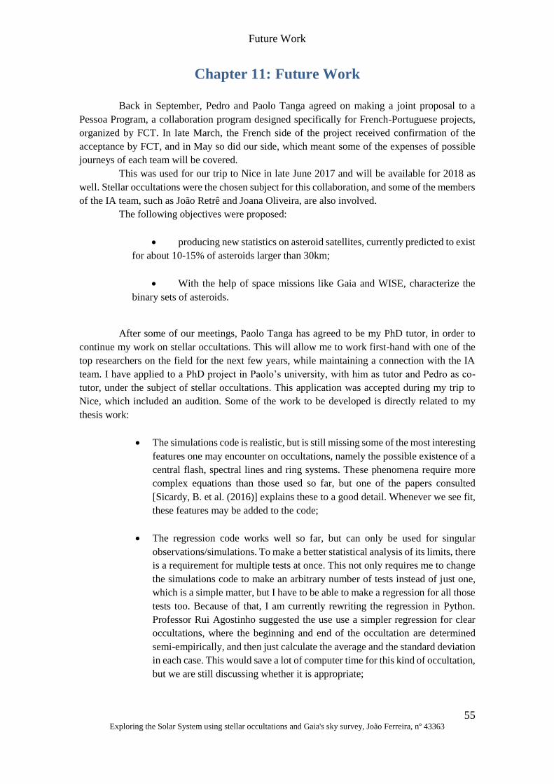
Future Work
55 Exploring the Solar System using stellar occultations and Gaia's sky survey, João Ferreira, nº 43363
Chapter 11: Future Work
Back in September, Pedro and Paolo Tanga agreed on making a joint proposal to a
Pessoa Program, a collaboration program designed specifically for French-Portuguese projects,
organized by FCT. In late March, the French side of the project received confirmation of the
acceptance by FCT, and in May so did our side, which meant some of the expenses of possible
journeys of each team will be covered.
This was used for our trip to Nice in late June 2017 and will be available for 2018 as
well. Stellar occultations were the chosen subject for this collaboration, and some of the members
of the IA team, such as João Retrê and Joana Oliveira, are also involved.
The following objectives were proposed:
• producing new statistics on asteroid satellites, currently predicted to exist
for about 10-15% of asteroids larger than 30km;
• With the help of space missions like Gaia and WISE, characterize the
binary sets of asteroids.
After some of our meetings, Paolo Tanga has agreed to be my PhD tutor, in order to
continue my work on stellar occultations. This will allow me to work first-hand with one of the
top researchers on the field for the next few years, while maintaining a connection with the IA
team. I have applied to a PhD project in Paolo’s university, with him as tutor and Pedro as co-
tutor, under the subject of stellar occultations. This application was accepted during my trip to
Nice, which included an audition. Some of the work to be developed is directly related to my
thesis work:
• The simulations code is realistic, but is still missing some of the most interesting
features one may encounter on occultations, namely the possible existence of a
central flash, spectral lines and ring systems. These phenomena require more
complex equations than those used so far, but one of the papers consulted
[Sicardy, B. et al. (2016)] explains these to a good detail. Whenever we see fit,
these features may be added to the code;
• The regression code works well so far, but can only be used for singular
observations/simulations. To make a better statistical analysis of its limits, there
is a requirement for multiple tests at once. This not only requires me to change
the simulations code to make an arbitrary number of tests instead of just one,
which is a simple matter, but I have to be able to make a regression for all those
tests too. Because of that, I am currently rewriting the regression in Python.
Professor Rui Agostinho suggested the use use a simpler regression for clear
occultations, where the beginning and end of the occultation are determined
semi-empirically, and then just calculate the average and the standard deviation
in each case. This would save a lot of computer time for this kind of occultation,
but we are still discussing whether it is appropriate;
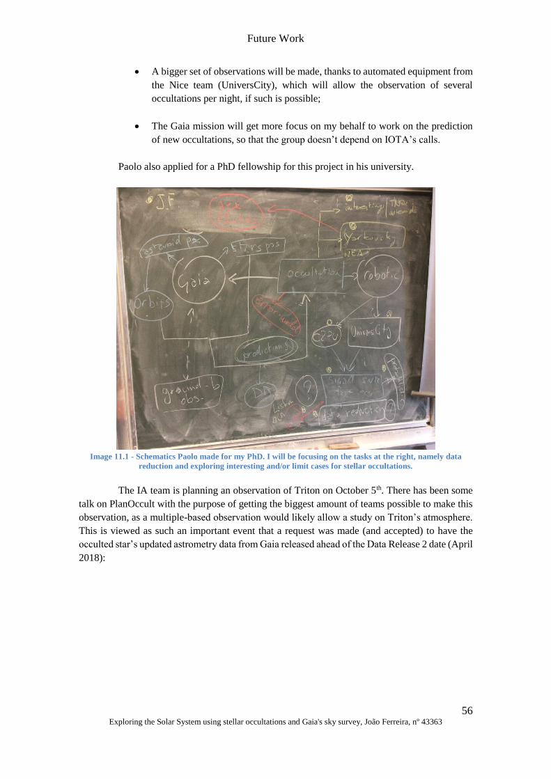
Future Work
56 Exploring the Solar System using stellar occultations and Gaia's sky survey, João Ferreira, nº 43363
• A bigger set of observations will be made, thanks to automated equipment from
the Nice team (UniversCity), which will allow the observation of several
occultations per night, if such is possible;
• The Gaia mission will get more focus on my behalf to work on the prediction
of new occultations, so that the group doesn’t depend on IOTA’s calls.
Paolo also applied for a PhD fellowship for this project in his university.
Image 11.1 - Schematics Paolo made for my PhD. I will be focusing on the tasks at the right, namely data
reduction and exploring interesting and/or limit cases for stellar occultations.
The IA team is planning an observation of Triton on October 5th. There has been some
talk on PlanOccult with the purpose of getting the biggest amount of teams possible to make this
observation, as a multiple-based observation would likely allow a study on Triton’s atmosphere.
This is viewed as such an important event that a request was made (and accepted) to have the
occulted star’s updated astrometry data from Gaia released ahead of the Data Release 2 date (April
2018):
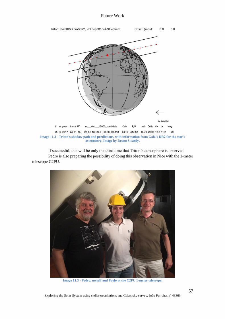
Future Work
57 Exploring the Solar System using stellar occultations and Gaia's sky survey, João Ferreira, nº 43363
Image 11.2 - Triton's shadow path and predictions, with information from Gaia’s DR2 for the star’s
astrometry. Image by Bruno Sicardy.
If successful, this will be only the third time that Triton’s atmosphere is observed.
Pedro is also preparing the possibility of doing this observation in Nice with the 1-meter
telescope C2PU.
Image 11.3 - Pedro, myself and Paolo at the C2PU 1-meter telescope.
Future Work
58 Exploring the Solar System using stellar occultations and Gaia's sky survey, João Ferreira, nº 43363
As mentioned in the “Observations” chapter, Neptune is the only planet of the Solar
System I have never observed through a telescope. This observation might change that, as
Neptune will be in the field of observation, and thanks to stellar occultations, I will have observed
every planet on our Solar System.
An earlier occultation for the group is predicted for August 28th, the target being the
asteroid Marion. This will be observable in Constância and Coimbra.
Right now, there are no other concrete observations planned, but the group agreed to
observe a total of at least 4 occultations throughout 2017.
A long-term personal objective is to make connections between my work developed in
the stellar occultations field and similar studies for exoplanets. Since stellar occultations share
several similarities with planetary transits, another area that interests me, I will be looking for an
opportunity on that field.
Bibliography
59 Exploring the Solar System using stellar occultations and Gaia's sky survey, João Ferreira, nº 43363
Bibliography
Theory:
Ortiz, J. L. Et al. (2014). Lessons learned from stellar occultations by Trans-Neptunian
Objects and prospects for the future, European Planetary Science Congress;
Santos-Sanz, P. et al. (2014). Characterization of trans-neptunian objects from thermal
radiometry and stellar occultations;
Desmars, J. (2015). Orbit determination of Trans-neptunian objects and Centaurs for
the prediction of stellar occultations, Astronomy and Astrophysics;
Gaia collaboration (2016). The Gaia Mission, Astronomy and Astrophysics;
Devogèle, M. et al (2015). A method to search for large scale concavities in asteroid
shape models, Monthly Notices of the Royal Astronomical Society;
Knuth, D. (1981). The Art of Computer Programming, Volume 2, Addison-Wesley.
Tyson, Neil (2009). The Pluto Files, W. W. Norton & Co., 2nd Edition.
Occultation results mentioned in the Introduction:
Sicardy, B. et al. (2003). Large changes in Pluto’s atmosphere as revealed by recent
stellar occultations, Nature;
Sicardy, B. et al. (2006). Charon’s size and upper limit on its atmosphere from a stellar
occultation, Nature;
Sicardy, B. et al. (2011).A Pluto-like radius and a high albedo for the dwarf planet Eris
from an occultation, Nature;
Braga-Ribas, F. et al. (2014). A ring system detected around the Centaur (10199)
Chariklo, Nature;
Ortiz, J. L. et al. (2012). Albedo and atmospheric constraints of dwarf planet Makemake
from a stellar occultation, Nature.
Current Research:
Boissel, Y. Et al (2014). An exploration of Pluto’s environment through stellar
occultations, Astronomy and Astrophysics;
Camargo, J.I.B. et al (2014). Candidate stellar occultations by Centaurs and trans-
Neptunian objects up to 2014, Astronomy and Astrophysics;
Alvarez-Candal, A. et al (2014). Stellar occultation by (119951) 2002 KX14 on April
26, 2012, Astronomy and Astrophysics;
Santos-Sanz et al (2015). JWST observations of stellar occultations by solar system
bodies and rings, Publications of the Astronomical Society of the Pacific;
Dias-Oliveira, A. et al (2015). Pluto's atmosphere from stellar occultations in 2012 and
2013, The Astrophysical Journal;
Benedetti-Rossi, G. et al (2016). Results from the 2014 November 15th multi-chord
stellar occultation by the TNO (229762) 2007 UK126, The Astronomical Journal;
Bibliography
60 Exploring the Solar System using stellar occultations and Gaia's sky survey, João Ferreira, nº 43363
Sicardy, B. et al (2016). Pluto’s atmosphere from the 29 June 2015 ground-based stellar
occultation at the time of the New Horizons flyby, The Astrophysical Journal;
Sicardy, B. (2016). Rings beyond the giant planets, Cambridge University Press;
Schindler, K. (2016). Results from a triple chord stellar occultation and far-infrared
photometry of the trans-Neptunian object (229762) 2007 UK126, Astronomy and Astrophysics;
Berard, D. et al (2017). The structure of Chariklo's rings from stellar occultations, The
Astronomical Journal;
Dias-Oliveira, A. et al (2017). Study of the plutino object (208996) 2003 AZ84 from
stellar occultations: size, shape and topographic features, The Astronomical Journal;
Gomes-Júnior, A.R. et al (2016). New orbits of irregular satellites designed for the
predictions of stellar occultations up to 2020, based on thousands of new observations, Monthly
Notices of the Royal Astronomical Society;
Frappa, E. et al (2011). Euraster an European Network for Asteroid Stellar Occultations,
EPSC-DPS Joint Meeting 2011;
Tanga, P. et al (2008). Asteroid occultations today and tomorrow: toward the GAIA era,
Astronomy and Astrophysics.
IOTA homepage: http://www.iota-es.de/;
PlanOccult info page: http://vps.vvs.be/mailman/listinfo/planoccult;
Kepler Space Telescope homepage: https://kepler.nasa.gov/;
NASA exoplanets archive: http://exoplanetarchive.ipac.caltech.edu/;
University of California’s exoplanet archive: http://exoplanets.org/;
European exoplanets archive: http://exoplanet.eu/;
Starry Night webpage: https://starrynight.com/starry-night-7-professional-astronomy-
telescope-control-software.html;
AVerMedia EZMaker 7: http://www.toptenreviews.com/computers/peripherals/best-
vhs-to-dvd-converters/avermedia-dvd-ezmaker-review/;
StarTech SVID2USB23: http://occultations.org/observing/educational-
materials/equipment/analog-video-recording-in-windows/;
DIGITUS DA-70820: https://driverscollection.com/?H=DA-70820&By=DIGITUS.
Gaia details and Data Release:
Gaia Collaboration et al. (2016). Gaia Data Release 1: Summary of the astrometric,
photometric, and survey properties, Astronomy and Astrophysics;
Lindegren, L. et al. (2016). Gaia Data Release 1: Astrometry – one billion positions,
two million proper motions and parallaxes, Astronomy and Astrophysics;
Todd, M. et al (2014). Predictions for the Detection of Earth and Mars Trojan Asteroids
with the Gaia Satellite, Monthly Notices of the Royal Astronomical Society;
Tanga, P. Gaia and the Solar System;
ESA’s Gaia homepage: http://sci.esa.int/gaia/.
Tangra and other popular lightcurve software:
Tangra homepage: http://www.hristopavlov.net/Tangra3/;
Occult 4 homepage: http://www.lunar-occultations.com/iota/occult4.html;
http://occultations.org/observing/educational-materials/equipment/analog-video-recording-in-windows/
Bibliography
61 Exploring the Solar System using stellar occultations and Gaia's sky survey, João Ferreira, nº 43363
Limovie: http://astro-limovie.info/limovie/limovie_en.html;
Astroart: http://www.msb-astroart.com/;
Grapher: http://www.goldensoftware.com/products/grapher.

Bibliography
62 Exploring the Solar System using stellar occultations and Gaia's sky survey, João Ferreira, nº 43363
Appendix
63 Exploring the Solar System using stellar occultations and Gaia's sky survey, João Ferreira, nº 43363
Appendix
List of abbreviations (Alphabetical Order)
Institutions
CAAUL – Centro de Astronomia e Astrofísica da Universidade de Lisboa;
CCV – Centro Ciência Viva;
FCT – Fundação para a Ciência e a Tecnologia;
FCUL – Faculdade de Ciências da Universidade de Lisboa;
IA – Institute of Astrophysics and Space Sciences;
IOTA-ES – International Occultation Timing Association – European Section.
Technical terms (Alphabetical Order)
AOTA – Asteroid Occultation Time Analyzer;
.csv – Comma Separated Values file;
DNR – Drop-to-noise ratio;
EPSC-DPS – European Planetary Science Congress – Division for Planetary Sciences.
FOV – Field Of View;
FPS – Frames Per Second;
Grapher – Computer program designed specifically to make plots.
J2000 – Celestial coordinates catalogue from January 1st 2000. J stands for “Julian”, as
in “Julian Calendar”, instead of Gregorian;
mas – Miliarcsecond;
Mathematica – Software developed by Wolfram Research. Its homepage is
https://www.wolfram.com/mathematica/;
NEO – Near Earth Object;
PSF – Point Spread Function;
Appendix
64 Exploring the Solar System using stellar occultations and Gaia's sky survey, João Ferreira, nº 43363
TNO/OTN – Trans-Neptunian Object/Objectos Trans-Neptunianos;
List of definitions (Alphabetical Order):
Air mass – Volume of air. In astronomy, the amount of atmosphere between the star
and the observer. At minimum, its value is 1 (in the zenith), and grows towards the horizon. The
bigger the air mass, the fainter and more distorted the signal will be;
Albedo – Fraction of the received sunlight reflected by a body’s surface;
Centaur – Minor/ dwarf planet between Jupiter and Neptune;
Drop-to-noise ratio – Comparison between the flux drop and the standard deviation of
the flux noise during an observation: Drop/Noise. If DNR < 1, it is said that the drop is within the
observation noise, and it shouldn’t be observable;
Equatorial coordinates – Right ascension and declination. This system uses Earth’s
equator as the celestial equator and Earth’s axis as the North Pole;
Horizontal coordinates – Altitude and azimuth. This system uses the local zenith as
the North Pole and the horizon as equator. The North cardinal direction is the azimuth zero point;
Lagrangian point – Spot in the orbital configuration of two massive bodies (like Earth
and the Sun) where a small object (like a satellite) can maintain a stable position in relation to
them, if only affected by gravity. There are 5 Lagrangian points in the Sun-Earth system;
Magnitude – Logarithmic unit of measurement of a star’s brightness. In this work,
“magnitude” refers to the apparent magnitude, connected to the luminosity of a star and the
distance separating us from it. Not to be confused with absolute magnitude, which is the apparent
magnitude of a star if we consider it to be 10 pc away. 5 magnitude units correspond to a
brightness difference factor of 100;
pc – Parsec. Unit of distance. Approximately 3*1016 m;
Spectro-photometry – Measurement of the spectrum of a star (or another object) with
the flux scale calibrated as a function of wavelength. Usually the results are compared with a
standard star, and the effects caused by Earth’s Atmosphere are corrected;
Zenith – Imaginary point in the sky directly above the observer.


![Projeto de sistema crítico para transmissão de vídeo em um ... · requirements that make the system works by using a link budget procedure. ... combustível[1]. aleV ressaltar](https://static.fdocumentos.tips/doc/165x107/5c9cf57488c993a1348bf20e/projeto-de-sistema-critico-para-transmissao-de-video-em-um-requirements.jpg)