1

Clique Communities in Social Networks

Luís Cavique, Universidade Aberta, Portugal, lcavique@univ-ab.pt

Armando B. Mendes, Universidade Açores, Portugal, amendes@uac.pt

Jorge M.A. Santos, Universidade Évora, Portugal, jmas@uevora.pt

1 Introduction

After Tim Berners-Lee's (2006) communication on the three ages of the

Web in the International World Wide Web Conference WWW2006, there has

been an explosion of interest in the social networks associated with Web 2.0 in

an attempt to improve socializing and come up with a new model for

knowledge management. Even though Tim Berners-Lee had imagined a read-

and-write Web, the Web was originally a read-only medium for the majority of

the users. As Mika (2007) describes it, the Web of the nineties was much like

the combination of a phone book and the yellow pages, a mix of individual

postings and corporate catalogues, and instilled a little sense of community

among its users.

Social Network Analysis is a very relevant technique that has emerged

in modern sociology, and which studies the interaction between individuals and

organizations. See Scott and Carrington (2011) and Wasserman and Faust

(1995) for the theoretical basis and key techniques in social networks.

The idea of ‘social network’ was loosely used for over a century to

connote complex sets of relationships between members of social systems at

all scales, from interpersonal to international (Freeman 2004). In 1954, J. A.

Barnes used the term systematically to denote patterns of ties, and is normally

considered the father of that expression. However, the visual approach to

measuring social relationships using graphs, known as sociograms, was

presented by Jacob Moreno (1934). In Moreno’s network, the nodes represent

individuals, while the edges stand for personal relationships. This scientific

area of sociology tries to explain how diffusion of innovation works, why

alliances and conflicts are generated in groups, how the leadership emerges

and how the group structure affects the group efficacy (Mika 2007).

2

A major development on the structure of social networks came from a

remarkable experiment by the American psychologist Stanley Milgram

(Milgram 1967). Milgram’s experiment consisted in sending letters from people

in Nebraska, in the Midwest, to people in Boston, on the East Coast, where the

latter were instructed to pass on the letters, by hand, to someone else they

knew. The letters that reached the destination were passed by around six

people. Milgram concluded that the experiment showed that, on average,

Americans are no more than six steps away from each other. This experiment

led to the concepts of the six degrees of separation and the notion of small-

world.

An interesting example of a small-world is the ‘Erdös Number’

(Grossman et al., 2007). Erdös is the most prolific mathematician, being author

of more than 1500 papers with more than 500 co-authors. Erdös is the number

zero and the researchers who worked with him are called Erdös number 1.

The co-authors of Erdös number 1 are the Erdös number 2, and so on,

building one of the oldest small-world known. The work of Erdös and Renyi

(1959) describes interesting properties of random graphs. A brand new interest

has been revived with the Watts and Strogatz (1998) model, published in the

Nature journal, which studies graphs with small-world properties and power-

law degree distribution.

The social network analysts need to survey each person about their

friends, ask for their approval to publish the data and keep a trace of that

population for years. Also, the applications, implemented on internet, that uses

the concept of establishing links between friends and friends of friends, like

Facebook or LinkedIn (LinkedIn Corporation), provide the required data.

According to Linton Freeman’s comprehensive Development of Social Network

Analysis, the key factors defining the modern field of social network analysis

are: the insight that the structure of networks affects the outcome of aggregate

actions, and the methodological approach that uses systematic empirical data,

graphic representation, and mathematical and computational models to

analyze networks. These attributes of social network analysis were established

through the work of scientists from the fields of psychology, anthropology, and

mathematics over the last decades (Freeman 2004).

3

The visualization of a small number of vertices can be completely

mapped. However, when the number of vertices and edges increases, the

visualization becomes incomprehensible. The large amount of data extracted

from the Internet is not compatible with the complete drawing. There is a

pressing need for new pattern recognition tools and statistical methods to

quantify large graphs and predict the behavior of network systems.

Graph mining can be defined as the science and the art of extracting

useful knowledge, like patterns and outliers provided, respectively, by repeated

and sporadic data, from large graphs or complex networks (Faloutsos et al.,

1999; Cook and Holder, 2007). As these authors put it, there are many

differences between graphs; however, some patterns show up regularly, the

main ones appearing to be: the small worlds, the degree distribution and the

community mining.

In this chapter, the clique communities are studied using the graph

partition approach, based on the k-clique structure. A k-clique is a relaxed

clique, i.e., a k-clique is a quasi-complete sub-graph. A k-clique in a graph is a

sub-graph where the distance between any two vertices is no greater than k. It

is a relevant structure to consider when analyzing large graphs like the ones

arising in social network analysis.

The proposed Socratic questioning is the following: How many k-clique

communities are needed to cover the whole graph? This work is part of a

larger project on common knowledge of proverbs whose previous results were

published in Mendes, Funk, Cavique (2010).

2 Graph Theory Concepts

The representation of social networks has been quite influenced by

graph theory. In the social networks, the set of vertices (or nodes) correspond

to the “actors” (i.e. people, companies, social actors) and the set of edges to

the “ties” (i.e. relationships, associations, links).

The sociologic applications of cohesive subgroups can include groups

such as work groups, sport teams, political party, religious cults, or hidden

structures like criminal gangs and terrorist cells. In this section, some concepts

about cohesive subgroups like cliques and relaxed cliques, such as k-clique, k-

club/k-clan and k-plex, are explained.

4

2.1 Graph notation

Graph theory has many applications and has been used for centuries.

The book by Berge (1958), called “Théorie des Graphes e ses Aplications”,

published many of the knowledge known at the time. A latter edition, in 1973,

established a very common notation in graph theory literature that is also used

in this chapter.

In this notation, an undirected graph is represented by G=(V,A), where

A⊆[V]2 is a pair in which V(G) represents the set of vertices or nodes, and

A(G), the set of links or edges. An edge can be also represented by {i, j}∈A(G),

where i and j are the two connected vertices. The number of vertices V(G) can

be represented by |V(G)| and the graph called of order n if V(G)={1,2,…,n} and

so, |V(G)|=n. The number of arcs m is given by the cardinality of A(G), i.e.

|A(G)|. If two vertices are joined by an edge, they are adjacent.

A graph G’=(V’, A’) is a sub-graph of the graph G=(V,A) if V’⊆V and

A’⊆A. We can also say that if C is a proper subset of V, than G’=G-C denotes

the sub-graph induced from G by deleting all vertices in C and their incident

edges. In Figure 1. the graph G’ is a sub-graph induced by G, while G’’ is not,

as only edges are missing.

G G’ G’’

Figure 1 Graph G and two sub-graphs G’ and G’’.

In Social Network Analysis, the order of the end-vertices of an edge is

usually irrelevant and so, we have to work only with undirected graphs. In

directed graphs, each directed edge (usually, called arc), has an origin and a

destination, and is represented by an ordered pair. In social network contexts,

the direction of an edge is not relevant; what is important is to acknowledge

the existence, or not, of a link between the edges.

5

2.2 Clique

Given an undirected graph G=(V, E), where V denotes the set of

vertices and E, the set of edges, the graph G1= (V1, E1) is called a sub-graph

of G, if V1⊆V, E1⊆E and for every edge (vi, vj)∈ E1, the vertices vi,vj∈ V1. A

sub-graph G1 is said to be complete, if there is an edge for each pair of

vertices. In fact, a clique is a complete sub-graph, which means that in a

clique, each member has direct ties with each other member or node. Some

simple examples of these very cohesive structures are shown in Figure . A

clique is maximal, if it is not contained in any other clique. The clique number

of a graph is equal to the cardinality of the largest clique of G and it is obtained

by solving the maximum clique NP-hard problem.

Figure 2 Cliques with 1, 2, 3, 4, 5 and 6 vertices.

The clique structure, where there must be an edge for each pair of

vertices, shows many restrictions in real life modeling and is uncommon in

social networks. So, alternative approaches for little more relaxed cohesive

groups were suggested, such as k-clique, k-clan/k-club and k-plex.

2.3 k-clique

Luce (1950) introduced the distance base cohesion groups called k-

clique, where k is the maximum path length between each pair of vertices. A

k-clique is a subset of vertices C such that, for every i, j∈ C, the distance d(i, j)

≤ k. The 1-clique is identical to a clique, because the distance between the

vertices is one edge. The 2-clique is the maximal complete sub-graph with a

path length of one or two edges. The path distance of two can be exemplified

by the “friend of a friend” connection in social relationships. In social websites,

like the LinkedIn, each member can reach his own connections as well as the

6

ones two and three degrees away. The increase of the value k corresponds to

a gradual relaxation of the criterion of clique membership. See Figure 2.

Figure 3 Examples with four nodes of 1-clique, 2-clique and 3-clique.

2.4 k-clan and k-club

A limitation of the k-clique concept is that some vertices may be distant

from the group, i.e. the distance between two nodes, may correspond to a path

involving nodes that do not belong to the k-clique. To overcome this handicap

Alba (1973) and Mokken (1979) introduced the diameter-based cohesion

group concepts called k-club and k-clan. The length of the shortest path

between vertices u and v in G is denoted by the distance d(u,v). The diameter

of G is given by diam(G)= max d(u, v) for all u,v∈ V. To find all k-clan, all the k-

cliques Si must be found first, and then the restriction diam(G[S])≤ k applied to

remove the undesired k-cliques. In Figure 3, on the left, the 2-clique {1,2,3,4,5}

was removed because d(4,5)=3, i. e. the path 4—6—5 is not possible as node

6 does not belong to the sub-graph with the 2-cliques. Another approach to

these diameter models is the k-club, which is defined as a subset of vertices S

such that diam(G[S])≤ k. In the left graph of Figure 3, can be found two 2-

cliques: {1,2,3,4,5} and {2,3,4,5,6}, one 2-clan: {2,3,4,5,6} and three 2-clubs:

{1,2,3,4}, {1,2,3,5} and {2,3,4,5,6}.

Figure 4 2-clans, 2-clubs (left) and 3-plex (right).

7

2.5 k-plex

An alternative way of relaxing a clique is the k-plex concept which takes

into account the vertices degree. The degree of a vertex of a graph is the

number of edges incident on the vertex, and is denoted by deg(v). The

maximum degree of a graph G is the maximum degree of its vertices and is

denoted by ∆(G). On the other hand, the minimum degree is the minimum

degree of its vertices and is denoted by δ(G). A subset of vertices S is said to

be a k-plex, if the minimum degree in the induced sub-graph δ(G[S])≥ |S|− k. In

Figure , on the right, the graph has 6 vertices and so, |S|=6 and the degree of

vertices 1, 3, 4 and 5 does not exceed the value 3. Thus, the minimum degree

in the induced sub-graph δ(G[S]) is 3. For |S|=6, k=3 is obtained.

3. The Two Phase Algorithm

Complex network and graph mining metrics are essentially based on

low complexity computational procedures, like the diameter of the graph, the

degree distribution of the nodes and connectivity checking, underestimating

the knowledge of the graph structure components.

On the other hand, in the literature, many algorithms have been

developed for network communities. One of the first studies is given by the

Kernighan, Lin (1970) algorithm, which finds a partition of the nodes into two

disjoint subsets A and B of equal size, such that the sum of the weights of the

edges between nodes in A and B is minimized. Recent studies, based on

physics method, introduced the concept of clique percolation (Derenyi, Palla,

Vicsek 2005), where the network is viewed as a union of cliques.

In order to find the k-clique communities, a two-phase algorithm is

proposed. First, all the maximal k-cliques in the graph are found. Second, the

best subset of the k-cliques is chosen to cover the vertices of the graph.

To find all the maximal k-cliques in the graph, we use the kth power of

the graph G in such a way that we can use an already well known algorithm,

the maximum clique algorithm. The procedures described in the next flowchart

starts by transforming the graph and applying next a maximum clique

algorithm and finally, in phase two, applying a set covering algorithm.

8

Input: distance k and graph G

Output: k-clique cover

1. Find all maximal k-cliques in graph G

1.1. The kth power of graph G

1.2. Apply maximum clique algorithm

2. Find the cover of G with k-cliques

2.1. Apply set covering algorithm

Algorithm 1 - The two-phase algorithm.

3.1. Maximal k-cliques in graph G

The transformation of a graph G(V,E) into a graph such that for every

i,j∈V, the distance d(i, j) ≤ k, is denoted by graph G(V,E)k.

The G(V,E)k is obtained using the kth power of the graph G with the

same set of vertices as G and a new edge between two vertices if there is a

path of length at most k between them (Skiena 1990).

The Maximum Clique is a NP-hard problem that aims to find the largest

complete sub-graph in a given graph. In this approach, we intend to find a

lower bound for the maximization problem, based on the heuristics proposed

by Johnson (1974) and in the meta-heuristic that uses Tabu Search developed

by Soriano and Gendreau (1996). Part of the work described in this section

can also be found in Cavique, Rego and Themido (2002) and Cavique and Luz

(2009).

We define A(S) as the set of vertices that are adjacent to vertices of a

current solution S. Let n=|S| be the cardinality of a clique S and Ak(S) the

subset of vertices with k arcs incident in S. A(S) can be divided into subgroups

A(S) = ∪Ak(S), k=1,..,n.

The cardinality of the vertex set |V| is equal to the sum of the adjacent

vertices A(S) and the non-adjacent ones A0(S), plus |S|, resulting in |V|=

Σ|Ak(S)|+n, k= 0,.., n. For a given solution S, we define a neighborhood N(S) if

it generates a feasible solution S’.

In this work we are going to use three neighbourhood structures. For

the next flowchart consider the following notation:

9

N+ (S) = {S´: S´= S ∪{vi}, vi∈An(S)}

N– (S) = {S´: S´= S \{vi}, vi∈S}

N0 (S) = {S´: S´= S ∪{vi}\{vk}, vi∈ An-1(S), vk

∈S}

where S is the current solution, S*, the highest cardinality maximal clique

found so far, T, the tabu list and N(S), the neighborhood structures.

Input: graph Gk, complete sub-graph S

Output: clique S*

1. T=∅; S*=S;

2. while not end condition

2.1. if (N+(S)\T ≠ null) choose the maximum S’

2.2. else if (N0(S)\T ≠ null) choose the maximum S’; update T

2.2.1. else choose the maximum S’ in N–(S); update T

2.3. update S=S’

2.4. if (|S|>|S*|) S*=S;

3. end while;

4. return S*;

Algorithm 2 - The Tabu Heuristic for the Maximum Clique Problem

Finding a maximal clique in a graph Gk is the same as finding a maximal k-

clique in a graph G. To generate a large set of maximal k-cliques, a multi-start

algorithm is used, which calls the Tabu Heuristic for Maximum Clique Problem.

3.2. The k-cliques Cover

To understand the structure of a clique community of a network in the

previous work (Cavique, Mendes and Santos 2009), the minimum set covering

formulation was used.

The detailed analysis of the resulting solution, the set of k-cliques, an

excess of over-coverings can be found, which makes it hard to interpret the

clique communities. For each pair of k-cliques, the nodes that belong to both k-

cliques, are called “bridges” between the two communities. In the next figure,

the matrix shows the bridges between the 15 k-cliques, with k equal 3, for the

10

Erdos-97-1 dataset, where the large density of connections does not allow for

a clear interpretation of the network.

1 2 3 4 5 6 7 8 9 10 11 12 13 14 15

1 128 132 122 122 139 147 123 125 130 138 140 150 144 155

2 151 138 145 158 153 147 142 151 154 160 161 152 161

3 173 171 182 181 174 174 180 186 191 194 184 193

4 181 176 172 188 185 184 194 196 197 197 196

5 181 170 197 191 186 196 199 193 197 195

6 183 181 183 189 196 199 200 191 200

7 174 180 181 192 192 201 195 206

8 191 192 201 204 197 201 200

9 187 206 201 203 204 205

10 203 209 202 197 203

11 216 217 215 219

12 220 212 223

13 222 231

14 226

15

Figure 5 Bridges between the 15-set of k-cliques in the k3-Erdos-97-1 dataset

The minimum set covering algorithm generates 15 k-cliques, which

covers all the 283 nodes, but over-covering 252 nodes.

In this paper, we propose a trade-off between the covered and over-

covered nodes. The new metric finds the best solution when the number of

covered nodes does not exceed the number of over-covered ones. In other

words, the best solution is found when the difference between covered and

over-covered nodes is maximal.

11

-2

0

2

4

6

8

10

12

14

16

18

20

0 1 2 3 4 5

cover

over-cover

diference

Figure 6 Best trade-off solution happens when the difference is maximal

The k-clique cover algorithm implementation is composed of a

constructive step and a reduction step.

The input for the k-clique cover is a matrix where each line corresponds

to a node of the graph and each column, a k-clique covering a certain number

of nodes.

In the constructive step, the Clique Cover heuristic, proposed by

Kellerman (1973) and improved by Chvatal (1979), is used.

We consider the following notation: M [line, column] or M [vertex, k-

clique] for the input matrix, C for the cost vector of each column, V for the

vertex set of G(V,E) and S for the set covering solution.

Input: M [line, column], C, V

Output: the cover S

1. Initialize R=M, S=∅,

// Constructive Step

2. While R ≠ ∅ do

2.1. Choose the best line i*∈R such as |M(i*,j)|=min |M(i,j)| ∀j

2.2. Choose the best column j* that covers line i*

2.3. Update R and S, R=R\M(i,j*) ∀i, S=S∪{j*}

3. End while

4. Sort the cover S by descending order of costs

12

5. For each Si do if (S\Si is still a cover) then S=S\Si

// Reduction Step

6. While (over-cover > cover) do

6.1. Choose the column j* such as (over-cover > cover)

6.2. Remove column j*

7. End While

8. Return S

Algorithm 3 - The Heuristic for the k-clique covering.

In the constructive step, for each iteration, it is chosen a line to be

covered and the best column that covers that line. Then, the solution S and the

remaining vertex R, are updated. The chosen line is usually the line that is

more difficult to cover, i.e. the line that corresponds to fewer columns. After

reaching the cover set, the second step is for removing redundancy, by sorting

the cover in descending order of cost and checking if each k-clique is really

essential.

In the reduction step, the best trade-off solution is found by removing

the most over-covered k-cliques, i.e. the k-cliques with a high degree of nodes

over-covering.

This heuristic can be improved using a Tabu Search heuristic, by

alternating the constructive step with the removal of the most expensive

columns, finding a trajectory of solutions, as presented in Gomes, Cavique e

Themido (2006).

The solution obtained with the reduction step, decreases the number of

k-cliques that covered all the nodes, allowing for a better interpretation of the

network. The sub-covered (or not-covered) nodes are treated as outlier nodes

and thus not considered in the clique community analysis.

In order to get a better interpretability of the network data, this analysis

considers the k-cliques covered nodes as communities, the over-covered

nodes, as bridges between the communities and the not-cover nodes, as

outlier (or marginal) nodes.

13

3.3. Two numeric examples

In this section, two numeric examples will be presented to show the

constructive and the reduction steps.

To exemplify the constructive step, given a graph with 5 vertices and 4

edges with E={(1,2), (2,3), (3,4), (4,5)}, the second power of the graph, k=2, a

new graph with 5 vertices and 7 edges is obtained with k-E={(1,2), (1,3), (2,3),

(2,4), (3,4) ,(3,5),(4,5)}.

Figure 7 Example of a graph G and its transformation into a G2.

Running a multi-start algorithm with the maximum clique problem, three

maximal cliques of size 3 can be easily identified: (1,2,3), (2,3,4) and (3,4,5).

Figure 8 k-clique generation example.

Finally, running the k-cliques cover, in the constructive step of phase 2,

two subgroups are found that cover all the vertices. The 2-clique cover is equal

to two. Notice that the vertex number 3 appears in the two sets. In social

14

network analysis, this is called a “bridge”. Indeed, node 3, with distance 2 can

reach any other vertex.

Figure 9 2-sets of 2-cliques cover the whole graph.

The previous figure presents the two subsets solution, using a matrix

representation and a graph. For large graphs and a large number of subsets,

the graph visualisation gets worse. In these cases, a better general view is

attained, using the matrix representation, which is the output of the set

covering heuristic.

To show the reduction step of phase 2, let us use a graph with 18 nodes

that has a diameter equal to 6. To cover the whole graph with 3-clique, 3-sets

are needed.

Figure 10 3-sets of 3-clique are needed to cover the graph

15

The result of the constructive step is 3-sets/columns of 3-clique. In the

reduction step, the columns with a larger difference between the covered

nodes and the non-covered nodes, will be removed. In the example, one

column will be removed, and the final result is a 2-set of 3-cliques, with 2

nodes as bridges (7 and 8) and one marginal node, the node 12.

Figure 11 2-sets of 3-clique are needed to cover the graph

4. Applying the algorithm to actual data sets

To validate the two-phase algorithm, two groups of datasets were used,

the Erdös graphs and some clique DIMACS (1995) benchmark instances. In

the Erdös graphs, each node corresponds to a researcher, and two nodes are

adjacent if the researchers published together. The graphs are named

“ERDOS-x-y”, where “x” represents the last two digits of the year that the

graphs were created, and “y”, the maximum distance from Erdös to each

vertex in the graph. The second group of graphs contains some clique

instances from the second DIMACS challenge. These include the “brock”

graphs, which contain cliques “hidden” within much smaller cliques, making it

hard to discover cliques in these graphs. The “c-fat” graphs are a result of fault

diagnosis data.

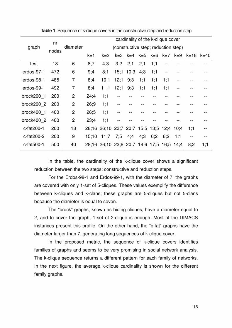
For the analysis of each graph, we consider the number of nodes, the

diameter and the cardinality of the set of k-cliques in the constructive and

reduction steps, varying k from 1 to the diameter, as showed in Table 1.

16

Table 1 Sequence of k-clique covers in the constructive step and reduction step

cardinality of the k-clique cover

(constructive step; reduction step) graph nr

nodes diameter

k=1 k=2 k=3 k=4 k=5 k=6 k=7 k=9 k=18 k=40

test 18 6 8;7 4;3 3;2 2;1 2;1 1;1 -- -- -- --

erdos-97-1 472 6 9;4 8;1 15;1 10;3 4;3 1;1 -- -- -- --

erdos-98-1 485 7 8;4 10;1 12;1 9;3 1;1 1;1 1;1 -- -- --

erdos-99-1 492 7 8;4 11;1 12;1 9;3 1;1 1;1 1;1 -- -- --

brock200_1 200 2 24;4 1;1 -- -- -- -- -- -- -- --

brock200_2 200 2 26;9 1;1 -- -- -- -- -- -- -- --

brock400_1 400 2 26;5 1;1 -- -- -- -- -- -- -- --

brock400_2 400 2 23;4 1;1 -- -- -- -- -- -- -- --

c-fat200-1 200 18 28;16 26;10 23;7 20;7 15;5 13;5 12;4 10;4 1;1 --

c-fat200-2 200 9 15;10 11;7 7;5 4;4 4;3 6;2 6;2 1;1 -- --

c-fat500-1 500 40 28;16 26;10 23;8 20;7 18;6 17;5 16;5 14;4 8;2 1;1

In the table, the cardinality of the k-clique cover shows a significant

reduction between the two steps: constructive and reduction steps.

For the Erdos-98-1 and Erdos-99-1, with the diameter of 7, the graphs

are covered with only 1-set of 5-cliques. These values exemplify the difference

between k-cliques and k-clans; these graphs are 5-cliques but not 5-clans

because the diameter is equal to seven.

The “brock” graphs, known as hiding cliques, have a diameter equal to

2, and to cover the graph, 1-set of 2-clique is enough. Most of the DIMACS

instances present this profile. On the other hand, the “c-fat” graphs have the

diameter larger than 7, generating long sequences of k-clique cover.

In the proposed metric, the sequence of k-clique covers identifies

families of graphs and seems to be very promising in social network analysis.

The k-clique sequence returns a different pattern for each family of networks.

In the next figure, the average k-clique cardinality is shown for the different

family graphs.

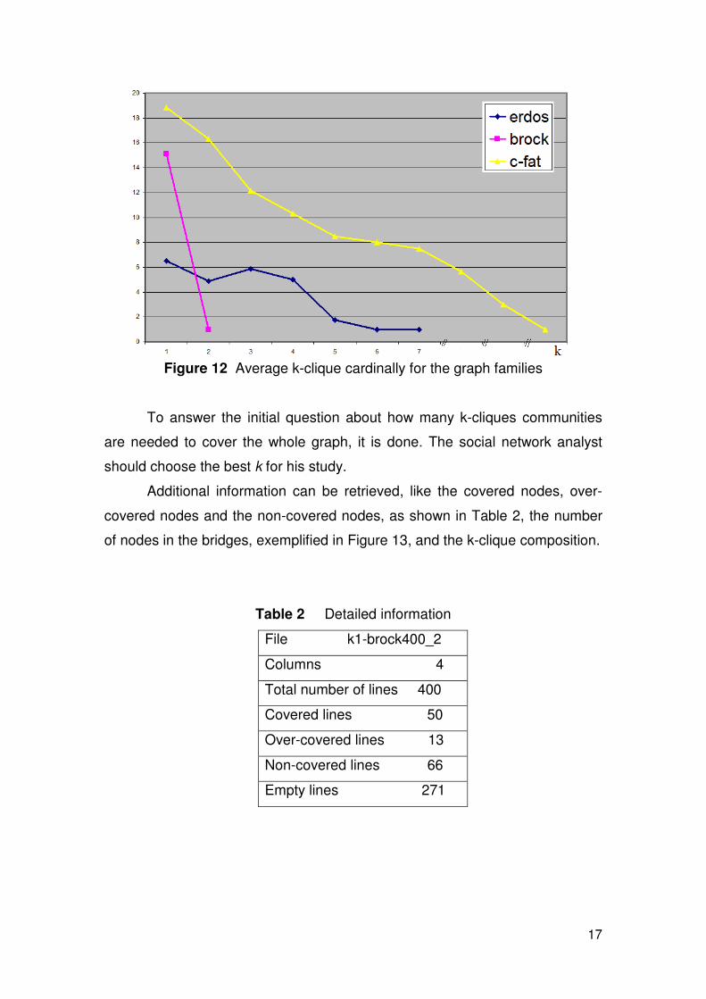
17

Figure 12 Average k-clique cardinally for the graph families

To answer the initial question about how many k-cliques communities

are needed to cover the whole graph, it is done. The social network analyst

should choose the best k for his study.

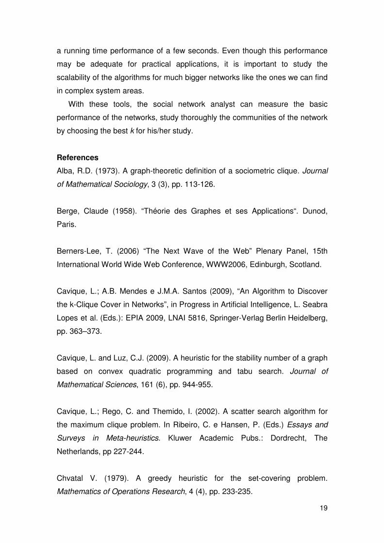
Additional information can be retrieved, like the covered nodes, over-

covered nodes and the non-covered nodes, as shown in Table 2, the number

of nodes in the bridges, exemplified in Figure 13, and the k-clique composition.

Table 2 Detailed information

File k1-brock400_2

Columns 4

Total number of lines 400

Covered lines 50

Over-covered lines 13

Non-covered lines 66

Empty lines 271

18

1 2 3 4

1 4 4 5

2 5 2

3 3

4

Figure 13 Bridges between the 4-set of k-cliques

in the k1-brock400_2 dataset

5. Conclusions

Given the large amount of data provided by the Web 2.0, there is a

pressing need to obtain new metrics to better understand the network

structure; how their communities are organized and the way they evolve over

time.

Complex network and graph mining metrics are essentially based on low

complexity computational procedures like the diameter of the graph, clustering

coefficient and the degree distribution of the nodes. The connected

communities in the social networks have, essentially, been studied in two

contexts: global metrics like the clustering coefficient and the node groups,

such as the graph partitions and clique communities.

In this work, the concept of relaxed clique is extended to the whole graph,

to achieve a general view, by covering the network with k-cliques. A graph

mining metric based on k-clique communities, allows for a better

understanding of the network structure.

In order to get a good interpretability of the network data, this analysis

considers the k-clique covered nodes as communities, the over-covered nodes

as bridges between the communities and the not-covered nodes as outlier

nodes. The k-clique cover algorithm implementation is composed of a

constructive step and a reduction step.

The sequence of k-clique communities is presented, where the diameter and

the community structure components are combined. The sequence analysis

shows that different graph families have different structures.

Social networks do not usually exceed a hundred nodes. In this work, the

proposed two-phase algorithm deals with graphs with hundreds of nodes, with

19

a running time performance of a few seconds. Even though this performance

may be adequate for practical applications, it is important to study the

scalability of the algorithms for much bigger networks like the ones we can find

in complex system areas.

With these tools, the social network analyst can measure the basic

performance of the networks, study thoroughly the communities of the network

by choosing the best k for his/her study.

References

Alba, R.D. (1973). A graph-theoretic definition of a sociometric clique. Journal

of Mathematical Sociology, 3 (3), pp. 113-126.

Berge, Claude (1958). “Théorie des Graphes et ses Applications“. Dunod,

Paris.

Berners-Lee, T. (2006) “The Next Wave of the Web” Plenary Panel, 15th

International World Wide Web Conference, WWW2006, Edinburgh, Scotland.

Cavique, L.; A.B. Mendes e J.M.A. Santos (2009), “An Algorithm to Discover

the k-Clique Cover in Networks”, in Progress in Artificial Intelligence, L. Seabra

Lopes et al. (Eds.): EPIA 2009, LNAI 5816, Springer-Verlag Berlin Heidelberg,

pp. 363–373.

Cavique, L. and Luz, C.J. (2009). A heuristic for the stability number of a graph

based on convex quadratic programming and tabu search. Journal of

Mathematical Sciences, 161 (6), pp. 944-955.

Cavique, L.; Rego, C. and Themido, I. (2002). A scatter search algorithm for

the maximum clique problem. In Ribeiro, C. e Hansen, P. (Eds.) Essays and

Surveys in Meta-heuristics. Kluwer Academic Pubs.: Dordrecht, The

Netherlands, pp 227-244.

Chvatal V. (1979). A greedy heuristic for the set-covering problem.

Mathematics of Operations Research, 4 (4), pp. 233-235.

20

Cook, D.J. e Holder, L.B. (Eds) (2007). “Mining Graph Data“. John Wiley &

Sons. DIMACS (1995). Maximum clique, graph coloring, and satisfiability,

Second DIMACS implementation challenge, URL http://dimacs.rutgers.edu/

Challenges/, accessed Mars 2011.

Derenyi I., G. Palla, T. Vicsek, (2005), Clique Percolation in Random

Networks, Physical Review Letters, vol. 94(16), pp. 160202.

Erdös, P., Renyi, A. (1959). On Random Graphs. I., Publicationes

Mathematicae, 6, pp. 290–297.

Faloutsos, M.; Faloutsos, P. and Faloutsos, C. (1999). On power-law

relationships of the Internet topology. In Proceedings of SIGCOMM. pp 251–

262.

Floyd, Robert W. (1962). Algorithm 97: Shortest Path. Communications of the

ACM, 5 (5), pp. 345.

Freeman, Linton C. (2004). The Development of Social Network Analysis: A

study in the sociology of science. Empirical Press.

Gomes, M.C.; L. Cavique; I.H. Themido (2006). The crew timetabling problem:

An extension of the crew scheduling problem. Annals of Operations Research,

144 (144), pp. 111-132.

Grossman, J.; Ion, P. and Castro, R. D. (2007) “The Erdös number Project”,

URL http://www.oakland.edu/enp/, accessed Mars 2011.

Johnson D.S. (1974). Approximation algorithms for combinatorial problems.

Journal of Computer and Systems Sciences, 9 (9), pp. 256-278.

Kellerman E. (1973). Determination of keyword conflict. IBM Technical

Disclosure Bulletin, 16(2), pp. 544–546.

21

Kernighan, B.W., Lin, Shen (1970). An efficient heuristic procedure for

partitioning graphs, Bell Systems Technical Journal, 49, pp. 291–307.

Luce, R.D. (1950). Connectivity and generalized cliques in sociometric group

structure. Psychometrika, 15 (15), pp. 159-190.

Mendes, A.; M. Funk and L. Cavique (2010). Knowledge discovery in the

virtual social network due to common knowledge of proverbs. In Weiss, Gary

M. and Stahlbock, Robert (Eds.) Proceedings of DMIN'10, 6th ed. CSREA

Press: USA, pp 213-219.

Mika, Peter (2007). Social Networks and the Semantic Web. Springer-Verlag.

Milgram, S. (1967). The Small World Problem. Psychology Today, 1 (1), pp.

60-67.

Mokken, R.J. (1979). Cliques, clubs and clans. Quality & Quantity, 13 (13), pp.

161-173.

Moreno, J. L. (1934). Who Shall Survive? Nervous and Mental Disease

Publishing Company, Washington D.C..

Scott, John P. and Carrington, Peter (Eds.) (2011). The SAGE Handbook of

Social Network Analysis. Sage Pubs.

Skiena, S. (1990). Implementing Discrete Mathematics: Combinatorics and

Graph Theory with Mathematica. Reading, MA: Addison-Wesley.

Soriano P.; Gendreau M. (1996) Tabu search algorithms for the maximum

clique, In: Johnson, D.S.; Trick, M.A. (Eds.). Clique, Coloring and Satisfiability,

Second Implementation Challenge DIMACS, American Mathematical Society,

pp. 221-242.

22

Wang N., S. Parthasarathy, K.-L. Tan, A.K.H. Tung (2008), CSV: visualizing

and mining cohesive subgraphs, in ACM SIGMOD ‘08 Proceedings,

Vancover, Canada.

Watts, D.J. and Strogatz, S.H. (1998). Collective dynamics of small-world

networks. Nature, 393 (393), pp. 409-410.

Wasserman, Stanley e Faust, Katherine (1995). Social Network Analysis:

Methods and applications. Cambridge University Press.